Byzantine-Robust Gossip: Insights from a Dual Approach

Renaud Gaucher    Aymeric Dieuleveut    Hadrien Hendrikx
Abstract

Distributed approaches have many computational benefits, but they are vulnerable to attacks from a subset of devices transmitting incorrect information. This paper investigates Byzantine-resilient algorithms in a decentralized setting, where devices communicate directly with one another. We leverage the so-called dual approach to design a general robust decentralized optimization method. We provide both global and local clipping rules in the special case of average consensus, with tight convergence guarantees. These clipping rules are practical, and yield results that finely characterize the impact of Byzantine nodes, highlighting for instance a qualitative difference in convergence between global and local clipping thresholds. Lastly, we demonstrate that they can serve as a basis for designing efficient attacks.

Machine Learning, Decentralized optimization, Byzantine Robustness, ICML

1 Introduction

As datasets become larger and more widely distributed across computing devices, distributed optimization becomes increasingly important. Decentralized optimization offers a solution to leverage the distributed computing power without suffering from communication bottlenecks or privacy leaks induced by a central server. However, communicating with large numbers of low-confidence devices opens up new security problems. Optimization can be thwarted by devices that send malicious messages, either deliberately because they are controlled by hostile parties, or because software and hardware problems cause them to behave incorrectly. We consider the problem of optimizing a finite sum of local functions distributed over the nodes of a network, where we assume some nodes to be Byzantine: instead of properly executing the algorithm, they modify their messages to disturb the optimization procedure. Robustness to Byzantine attacks is a worst-case scenario in the sense that we model adversarial nodes as omniscient, able to collude, and capable of sending different information to different nodes (Lamport et al., 1982; Blanchard et al., 2017)

We assume that $n$ nodes are linked by a communication network which we represent as an undirected graph $\mathcal{G}=(\mathcal{V},\mathcal{E})$, with $\mathcal{V}=\{1,\dots,n\}$ the vertices and $\mathcal{E}$ the edges. In the Byzantine context, nodes (i.e. vertices) are split into honest nodes $\mathcal{V}_{h}$ and Byzantine ones $\mathcal{V}_{b}$. Note that since Byzantine nodes are assumed to be omniscient and can send any values, edges between Byzantine nodes do not matter: they do not provide them additional information nor allow them to send different messages. Therefore, we only consider honest-to-honest edges $\mathcal{E}_{h}$, and honest-to-Byzantine ones $\mathcal{E}_{b}$. We always assume the subgraph of honest nodes $\mathcal{G}_{h}:=(\mathcal{V}_{h},\mathcal{E}_{h})$ to be connected. For any $i\in\mathcal{V}_{h}$, we denote $f_{i}:\mathbb{R}^{d}\to\mathbb{R}$ the local objective function on node $i$. Then, the optimization problem writes:

$$\textstyle\min_{x\in\mathbb{R}^{d}}\sum_{i\in\mathcal{V}_{h}}{f_{i}(x)}.$$ (1)

We solve this problem in a decentralized way. Each node $i\in\mathcal{V}$ maintains and updates a local parameter $x_{i}\in\mathbb{R}^{d}$. We consider the standard gossip approaches (Boyd et al., 2006; Nedic & Ozdaglar, 2009; Duchi et al., 2011; Scaman et al., 2017), in which communication steps consist in performing local parameter averages between neighbors. This corresponds to applying a so-called gossip matrix that encapsulates the topology of the graph.

Such gossip algorithms naturally arise when solving a well-chosen dual formulation of Equation 1 with standard first-order methods. This dual approach gives a principled framework to design and analyze efficient decentralized algorithms, successfully enabling for instance acceleration (Scaman et al., 2017; Kovalev et al., 2020) or variance reduction (Hendrikx et al., 2019). In this paper, we investigate the benefits of this approach in the Byzantine robust setting.

Since its introduction by Blanchard et al. (2017), the setting of Byzantine-robust learning has been extensively studied. Yet,, most works focus on the federated case, in which all nodes directly communicate with a central server (Yin et al., 2018; Chen et al., 2017; Alistarh et al., 2018; Li et al., 2019; El-Mhamdi et al., 2020; Karimireddy et al., 2020, 2021; Farhadkhani et al., 2022), or in the fully connected case, in which any pair of agents may communicate (El-Mhamdi et al., 2021; Farhadkhani et al., 2023). These approaches typically rely on federated stochastic gradient methods, coupled with robust aggregation. In the federated case, specific attacks have been proposed by leveraging the stochasticity of the problem (Baruch et al., 2019; Xie et al., 2020).

While the centralized case has been studied extensively, the fully decentralized setting has received less attention. A keystone to Byzantine-robust decentralized learning is to find a robust approximate agreement, which has been studied in 2012-2014 (Vaidya et al., 2012; Vaidya, 2014; LeBlanc et al., 2013). Yet these works only focused on achieving agreement within the convex hull of the initial parameters, without seeking optimality. A few recent works have managed to propose Byzantine-robust decentralized learning algorithms. Such methods typically rely on adapting federated robust aggregation schemes (Peng et al., 2021; Fang et al., 2022). More recently, aggregation rules leveraging the difference of neighbors positions have been successfully proposed (He et al., 2022; Wu et al., 2023; Farhadkhani et al., 2023). We summarize the properties of these works in Table 1. However, despite sufficient robustness criteria for adapted rules (Wu et al., 2023; Kuwaranancharoen & Sundaram, 2023) and impossibility results (El-Mhamdi et al., 2021; He et al., 2022), a fine characterization of the influence of Byzantine nodes remains elusive, even for basic problems such as gossip averaging.

Practical Sparse $\mathcal{G}$ Convergence Dual
Farhadkhani et al. (2023)
He et al. (2022)
Wu et al. (2023)
Peng et al. (2021)
ECG - Global-Clipping
ECG -  Local-Clipping
Table 1: Comparison to main references. ECG holds for $\operatorname{\operatorname{EdgeClippedGossip}}$, i.e., Algorithm 1. Practical: indicates that the algorithmic rule can be used without oracle knowledge. Sparse $\mathcal{G}$: indicates that the methods can be used for any graph. Convergence: indicates that convergence is always ensured up to a neighborhood, generally of size $\delta_{\max}\zeta^{2}$. Dual: indicates that the algorithm is grounded in the dual approach.

Contributions. In this paper, (i) we demonstrate how the dual approach can be used to interpret clipped Gossip, an existing robust algorithm, as a clipped dual gradient descent, (ii) derive clipping rules for this algorithm, (iii) provide convergence guarantees to better understand their robustness (or there lack of) to Byzantine attacks. In particular, we highlight two main settings depending on whether we choose the clipping threshold locally or globally. We obtain non-asymptotic convergence results for both versions, and discuss pros and cons of each method. Note that that our clipping rules can be implemented in practice (assuming some coordination for the global one). (iv) We eventually propose a constructive approach to design attacks by exploiting the topology of the network.

Our main algorithm, $\operatorname{\operatorname{EdgeClippedGossip}}$, is defined for generic objective functions. Yet, we restrict its analysis to the problem of decentralized mean-estimation, which allows us to obtain tight convergence bounds. We insist on the fact that this seemingly simple problem is the base building block for all decentralized algorithms, and yet is far from being understood in the Byzantine setting. The general (convex) case is left as an important open problem, though the dual approach allows to efficiently disentangle communication and computation in decentralized optimization (Hendrikx et al., 2019; Kovalev et al., 2020), and is thus a promising approach for a next step.

Notations. We denote $\textbf{1}_{n}=(1,\ldots,1)^{T}$; $\|\cdot\|_{2}$ or simply $\|\cdot\|$ (resp. $\langle\cdot,\cdot\rangle$) the Euclidean norm (resp. inner product) on $\mathbb{R}^{d}$; $\|\cdot\|_{F}$ the Frobenius norm of any matrix in $\mathbb{R}^{d\times n}$, and $\langle M,N\rangle_{F}=\operatorname{Tr}(M^{T}N)$ the corresponding inner product. We denote $X_{i,:}$ the $i$-th row of a matrix $X$. For a matrix $M$ in $\mathbb{R}^{n\times d}$, we denote $\overline{M}:=n^{-1}\textbf{1}_{n}\textbf{1}_{n}^{T}M$, and for $p\in\{1,2,\infty\}$, we denote $\|M\|_{p,2}$, the $p$-norm of the vector of 2-norms of the rows of $M$, i.e., $\|(\|M_{i,:}\|_{2})_{i\leqslant n}\|_{p}$. Moreover, $C^{\dagger}$ is the Moore Penrose inverse of $C$ and $\operatorname{Id}$ is the identity matrix. We identify $\mathbb{R}^{\mathcal{E}}$ to $\mathbb{R}^{|\mathcal{E}|}$ and $\mathbb{R}^{\mathcal{V}}$ to $\mathbb{R}^{n}$. We denote the minimum between $a$ and $b$ as $a\wedge b$.

2 ClippedGossip and its dual interpretation

This section introduces a dual point of view on clipped gossip. We start by introducing the basics of gossip algorithms and their flaws in the Byzantine setting. Then, we present the algorithm proposed by He et al. (2022). Finally we derive our algorithm of interest, $\operatorname{\operatorname{EdgeClippedGossip}}$, which in a particular case recovers their algorithm enabling to reinterpret it as Clipped Gradient Descent in the dual.

Setting: We denote $n_{h}=|\mathcal{V}_{h}|$ and $n_{b}=|\mathcal{V}_{b}|$ the total number of honest and Byzantine nodes, and $N_{h}(i)$ and $N_{b}(i)$ the number of honest and Byzantine neighbors of node $i$. Each agent owns and iteratively updates a local parameter $x_{i}^{t}$. At time $t$, we denote $X^{t}:=[x_{1}^{t},\ldots,x_{n}^{t}]^{T}\in\mathbb{R}^{\mathcal{V}\times d}$ the parameter matrix, which can be split into honest and Byzantine parameter matrices by writing $X=\begin{pmatrix}X^{t}_{h}\\ X^{t}_{b}\end{pmatrix}$, where $X^{t}_{h}=[(x^{t}_{i})_{i\in\mathcal{V}_{h}}]^{T}$ (resp. $X^{t}_{b}$) is the sub-matrix containing the models held by the honest workers (resp. Byzantine). Note that Byzantine nodes (in opposition to malicious nodes) can declare different values to each of their neighbors. As such, only the number and positions of connections with Byzantine nodes matter, and we can w.l.o.g identify the number of edges linking Byzantine and honest nodes $|\mathcal{E}_{b}|$ to the number of Byzantine workers $n_{b}$.

2.1 Gossip - average consensus case

In gossip algorithms, information is shared between neighbors by performing local averaging steps. As previously explained, we focus on the average consensus problem, which is an important special case of Equation 1.

Definition 2.1 (Average consensus problem (ACP)).

The ACP consists in computing ${\overline{x^{*}}=\frac{1}{n_{h}}\sum_{i\in\mathcal{V}_{h}}x_{i}^{*}}$, where each node $i\in\mathcal{V}_{h}$ holds a value $x_{i}^{*}$. Equivalently, it consists in solving Problem (1) with $f_{i}(x)=\|x-x_{i}^{*}\|^{2}$.

We define a gossip matrix as follows:

Definition 2.2 (Gossip matrix, spectral gap).

A matrix ${W\in\mathbb{R}_{+}^{n\times n}}$ is a gossip matrix for a graph $\mathcal{G}=(\mathcal{V},\mathcal{E})$ if: (i) $W$ is symmetric and doubly-stochastic: $W\textbf{1}_{n}=\textbf{1}_{n}$, and $\textbf{1}_{n}^{T}W=\textbf{1}_{n}^{T}$. (ii) $W$ characterizes connections in the network: $W_{ij}\neq 0$ if and only if $i=j$ or ${(i\sim j)}\in\mathcal{E}$.

Such a $W$ has eigenvalues $1=\mu_{1}(W)\geqslant|\mu_{2}(W)|\geqslant\ldots\geqslant|\mu_{n}(W)|$. The spectral gap of $W$ is defined as $\gamma_{W}:=1-|\mu_{2}(W)|$. If the graph $\mathcal{G}$ is connected, then $\gamma_{W}>0$. The spectral gap is the main quantity characterizing the information propagation in the graph.

The standard gossip algorithm writes (Boyd et al., 2006):

$$X^{t+1}=WX^{t},$$ (2)

In the absence of Byzantine nodes, gossip averaging (Equation 2) ensures linear convergence of the parameters to the average (Boyd et al., 2006), with $X^{0}=(x_{i}^{*})_{i\in\mathcal{V}}$ at a linear rate: $\sum_{i\in\mathcal{V}}\|x_{i}^{t}-\overline{x^{*}}\|^{2}\leqslant(1-\gamma)^{2t}\sum_{i\in\mathcal{V}}\|x_{i}^{0}-\overline{x^{*}}\|^{2}.$

Example 2.3 (Gossip from Graph Laplacian).

Let us consider the Laplacian matrix of the graph $L=D-A$ where $D$ is the diagonal matrix of degrees and $A$ is the adjacency matrix (i.e., $A_{ij}=\mathds{1}_{{(i\sim j)}\in\mathcal{E}}$).

Then, $W_{L}=\operatorname{Id}-\eta L$ is a gossip matrix for $\eta\leqslant\frac{1}{\max_{i}(D_{ii})}$. We then have that $\gamma_{W_{L}}=\eta{\mu_{\min}^{+}(L)}$, with $\mu_{\min}^{+}(L)$ the smallest positive eigenvalue of $L$.

Unfortunately, standard gossip communications use non-robust averaging steps, and so they are vulnerable to a single Byzantine node, which can drive all honest nodes to any position (Blanchard et al., 2017).

2.2 Clipped gossip: gossiping robustly

To remedy this vulnerability problem, He et al. (2022) propose a computationally-efficient solution for robust gossip communication. Their algorithm extends self-centered clipping (Karimireddy et al., 2021) to the decentralized case: nodes project all parameters they receive on a ball centered on their own parameter. Formally, for $\tau\geqslant 0$ and $x\in\mathbb{R}^{d}$,

$$\operatorname{Clip}(x;\tau):=\frac{x}{\|x\|_{2}}\min(\|x\|_{2},\tau)$$ (3)

is the projection of $x$ onto the $L_{2}$ ball of radius $\tau$. Then, for $\boldsymbol{\tau}^{t}\in\mathbb{R}^{\mathcal{V}_{h}}$, He et al. (2022)’s communication algorithm, called $\operatorname{ClippedGossip}(\boldsymbol{\tau}^{t})$, writes:

$$\begin{cases}x_{i}^{t+1}=x_{i}^{t}+\sum_{j\in\mathcal{V}}W_{ij}\operatorname{Clip}(x_{j}^{t}-x_{i}^{t};\boldsymbol{\tau}_{i}^{t})\text{ if }i\in\mathcal{V}_{h}\\ x_{i}^{t+1}=\,*,\text{ i.e., is arbitrary,}\,\text{ if }i\in\mathcal{V}_{b}.\end{cases}$$ (ClippedGossip)

In the limit case of $\tau_{i}^{t}=\infty$ for all $t\geqslant 0$ and $i\in\mathcal{V}_{h}$ we recover the standard gossip averaging of Equation 2, which with Byzantines writes: $\begin{pmatrix}X^{t+1}_{h}\\ \ldots\end{pmatrix}=W\begin{pmatrix}X^{t}_{h}\\ X^{t}_{b}\end{pmatrix},$ where we denote by $\ldots$ the fact that we have no control on the models held by Byzantines, thus considered as arbitrary: $X_{b}^{t+1}=*$.

It can be shown that one step of $\operatorname{ClippedGossip}$ ensures robust contraction, which allows it to be used efficiently as a communication primitive for Byzantine-robust decentralized optimization. For instance, He et al. (2022) combine $\operatorname{ClippedGossip}$ with local computation steps (stochastic gradients with momentum) to solve Problem 1 for generic convex smooth functions $f_{i}$ in the decentralized Byzantine setting. Generic analyses also show that $\operatorname{ClippedGossip}$ allows Byzantine-Resilient Decentralized SGD to converge to a neighborhood of the optimum (Wu et al., 2023). More generally, the idea of self-centered clipping is at the heart of several Byzantine-robust methods (Gorbunov et al., 2022).

Remark 2.4 (Oracle clipping rule in He et al. (2022)).

To ensure their algorithm’s convergence, He et al. (2022) rely on an oracle clipping threshold, written for node $i\in\mathcal{V}_{h}$ as $\boldsymbol{\tau}_{i}^{t}:=\sqrt{\frac{1}{\delta(i)}\sum_{j\in\mathcal{V}_{h}}W_{ij}\mathbb{E}\|x_{i}^{t+1/2}-x_{j}^{t+1/2}\|^{2}_{2}},$ where $\delta(i)=\sum_{j\in\mathcal{V}_{b}}W_{ij}$ is the weight associated to Byzantine neighbors of node $i$ in the gossip matrix $W$, and $x_{i}^{t+1/2}$ is the local model after the optimization step. Not only does each node need to know the variance of the noise of its neighbors, but it also requires to know which nodes are honest. This breaks the fundamental assumption of not knowing the identity (honest or Byzantine) of the nodes. Even if it is only required for setting the clipping threshold, this is still a major problem since the clipping threshold is a very sensitive parameter, and it is unclear what happens, specifically in case of under-clipping. Experiments are performed using a rule of thumb for the clipping threshold, not supported by theory. In contrast, our approach leads to a computable clipping rule which is supported by theory.

2.3 Dual approach

As previously mentioned, the dual approach is very popular in decentralized learning (Jakovetić et al., 2020; Uribe et al., 2020), and is at the heart of key advances, such as acceleration (Scaman et al., 2017; Hendrikx et al., 2019; Kovalev et al., 2020) or variance reduction (Hendrikx et al., 2021). In this section, we show that $\operatorname{ClippedGossip}$ (He et al., 2022) can be understood as Clipped Gradient Descent in the dual, which we will then leverage for the analysis.

2.3.1 Byzantine-free dual approach.

We consider Problem (1) in a setting without Byzantine agents. We rewrite it as a constrained problem, introducing one model per agent and enforcing equality between neighbors – and thus on all nodes, using connectivity of $\mathcal{G}$:

$$\min_{x\in\mathbb{R}^{d}}\sum_{i\in\mathcal{V}}{f_{i}(x)}=\min_{\begin{subarray}{c}(x_{i})_{i\in\mathcal{V}}\in\mathbb{R}^{d\times\mathcal{V}}\\ \forall{(i\sim j)}\in\mathcal{E}\,x_{i}=x_{j}\end{subarray}}\sum_{i\in\mathcal{V}}{f_{i}(x_{i})}.$$ (4)

For $X\in\mathbb{R}^{\mathcal{V}\times d}$, we note $F(X)=\sum_{i\in\mathcal{V}}f_{i}(X_{i:})$, and encode the edge-wise constraint through a matrix ${C^{T}\in\mathbb{R}^{\mathcal{E}\times\mathcal{V}}}$, such that $[C^{T}X]_{{(i\sim j)},:}=X_{j:}-X_{i:}$ for any edge ${(i\sim j)}$ in $\mathcal{E}$. Therefore, we can rewrite Problem (4) as follows:

$$\min_{\begin{subarray}{c}X\in\mathbb{R}^{\mathcal{V}\times d},\ C^{T}X=0\end{subarray}}F(X).$$ (5)

Assuming all functions $f_{i}$ to be smooth and strongly convex, we can define $f_{i}^{*}:y\mapsto\sup_{x\in\mathbb{R}^{d}}\langle y,x\rangle-f_{i}(x)$ the Fenchel-Legendre transform of $f_{i}$. Similarly, for any $Y\in\mathbb{R}^{\mathcal{V}\times d}$, $F^{*}(Y):=\sup_{X\in\mathbb{R}^{\mathcal{V}\times d}}\langle X,Y\rangle_{F}-F(X)$, and so $F^{*}(Y)=\sum_{i\in\mathcal{V}}f_{i}^{*}(Y_{i:})$ since $F$ is separable. Using Lagrangian duality, the dual of Equation 5 writes:

$\displaystyle\min_{\begin{subarray}{c}X\in\mathbb{R}^{\mathcal{V}\times d}\\ C^{T}X=0\end{subarray}}F(X)$ $\displaystyle=\min_{\begin{subarray}{c}X\in\mathbb{R}^{\mathcal{V}\times d}\end{subarray}}\max_{\Lambda\in\mathbb{R}^{\mathcal{E}\times d}}F(X)-\langle\Lambda,C^{T}X\rangle_{F}$
$\displaystyle=-\min_{\Lambda\in\mathbb{R}^{\mathcal{E}\times d}}F^{*}(C\Lambda),$ (6)

where $\Lambda$ corresponds to Lagrangian multipliers. This dual problem can be solved by gradient descent with step-size $\eta$:

$$\Lambda^{t+1}=\Lambda^{t}-\eta C^{T}\nabla F^{*}(C\Lambda^{t}).$$ (7)

Denoting $Y:=C\Lambda\in\mathbb{R}^{\mathcal{V}\times d}$, this implies that

$\displaystyle Y^{t+1}$ $\displaystyle=Y^{t}-\eta CC^{T}\nabla F^{*}(Y^{t}).$ (8)

Equation 8 thus generalizes Gossip algorithms to generic functions $(f_{i})_{i=1,\dots,n}$, going beyond the case of average consensus described in Section 2.1. Indeed, the matrix $CC^{T}$ corresponds to the Graph Laplacian $L$ introduced in Example 2.3, and in the particular case of quadratic $f_{i}$, Equation 8 is equivalent to Equation 2 for $W_{L}=\operatorname{Id}-\eta L$.

In fact, Equation 8 operates a gossip procedure on the dual variable $Y^{t}$. The associated primal variable is defined as $X^{t}=\nabla F^{*}(Y^{t})=(\nabla f_{i}^{*}(y_{i}^{t}))_{i\in\mathcal{V}}^{T}$. Notations are summarized in Table 2. Convergence guarantees then follow from standard gradient analyses, and in particular $X^{t}$ converges linearly to the solution of Equation 5. Efficient gossip algorithms can be obtained by using other algorithms on the dual problem, leading for instance to accelerated (randomized) gossip (Scaman et al., 2017; Hendrikx et al., 2019).

Variable Name Size Rows
$X$ primal parameter $\mathcal{V}\times d$ $(x_{i})_{i\in\mathcal{V}}$
$Y$ dual parameter $\mathcal{V}\times d$ $(y_{i})_{i\in\mathcal{V}}$
$\Lambda$ Lagrange multipliers $\mathcal{E}\times d$ $(\lambda_{(i\sim j)})_{{(i\sim j)}\in\mathcal{E}}$
$C^{T}\nabla F^{*}(C\Lambda)$ Flow on the edges $\mathcal{E}\times d$ $(x_{i}-x_{j})_{{(i\sim j)}\in\mathcal{E}}$
Table 2: Summary of notations

2.3.2 Adaptation in the Byzantine setting.

We now discuss how to leverage the dual approach in the Byzantine setting. In the derivations above, the updates on the Lagrangian multipliers $\Lambda^{t}\in\mathbb{R}^{\mathcal{E}\times d}$ naturally model the information shared through edges. The flow of information itself can be written as $C^{T}\nabla F^{*}(C\Lambda)$, see Equation 7. In particular, each row of $\Lambda^{t}$ (resp. $C^{T}\nabla F^{*}(C\Lambda^{t})$) corresponds to the value (resp. flow) on a single edge ${(i\sim j)}\in\mathcal{E}$ of the graph. We naturally index rows by edges, and denote $\lambda_{{(i\sim j)}}^{t}$ the corresponding row, thus writing, ${\forall{(i\sim j)}\in\mathcal{E}}$, $\lambda_{{(i\sim j)}}^{t+1}=\lambda_{{(i\sim j)}}^{t}-\eta[\nabla f_{j}^{*}(y_{j}^{t})-\nabla f_{i}^{*}(y_{i}^{t})]$, using that:

$$(C^{T}\nabla F^{*}(C\Lambda^{t}))_{(i\sim j)}=\nabla f_{j}^{*}(y_{j}^{t})-\nabla f_{i}^{*}(y_{i}^{t}).$$ (9)

In other words, applying an operator on the update on the rows of $\Lambda$ correspond to altering the information transmitted between nodes. For example, setting the row $(C^{T}\nabla F^{*}(C\Lambda^{t}))_{{(i\sim j)}}$ to 00 corresponds to removing edge ${(i\sim j)}$ from the graph. We aim at leveraging this observation to guide the design of algorithms. In the following, we use clipping (Equation 3) to regulate the flow on edges.

Algorithm 1 Byzantine-Resilient Decentralized Optimization with $\operatorname{\operatorname{EdgeClippedGossip}}$ $(\boldsymbol{\tau}^{t})$
  Input: $\{f_{j}\}$, $\{y_{j}^{0}\}$, $\eta$, $\{\boldsymbol{\tau}^{t}\}$
  for $t=0$ to $T$ do
     for $j=1,\ldots,n$ in parallel do
        Compute $x_{j}^{t}=\nabla f_{j}^{*}(y_{j}^{t})$ if $j\in\mathcal{V}_{h}$ else $*$
        Share parameter $x_{j}^{t}$ with neighbors
        $\ y_{j}^{t+1}=y_{j}^{t}-\eta\sum_{i\sim j}\operatorname{Clip}\left(x_{j}^{t}-x_{i}^{t};\boldsymbol{\tau}^{t}_{{(i\sim j)}}\right)$
Oracle strategy.

If an oracle had access to the set of Byzantine edges $\mathcal{E}_{b}$, then applying $\forall{(i\sim j)}\in\mathcal{E}$,

$\displaystyle\!\!\lambda_{{(i\sim j)}}^{t+1}\!=\!\lambda_{{(i\sim j)}}^{t}-\!\eta\!\operatorname{Clip}(\nabla f_{j}^{*}(y_{j}^{t})\!-\!\nabla f_{i}^{*}(y_{i}^{t}),\tau_{{(i\sim j)}})$ (10)

with $\tau_{{(i\sim j)}}=\infty\times\mathds{1}_{{(i\sim j)}\notin\mathcal{E}_{b}}$ exactly recovers the generalized gossip algorithm in Equation 7 on the subgraph of honest nodes, and thus converges to the solution. Going beyond such an oracle strategy, we consider Equation 10 for a general vector $\boldsymbol{\tau}\in\mathbb{R}^{\mathcal{E}}$:

$\displaystyle\lambda_{{(i\sim j)}}^{t+1}=\lambda_{{(i\sim j)}}^{t}-\eta\operatorname{Clip}(\nabla f_{j}^{*}(y_{j}^{t})-\nabla f_{i}^{*}(y_{i}^{t}),\boldsymbol{\tau}_{{(i\sim j)}}).$

This gives Algorithm 1, called $\operatorname{\operatorname{EdgeClippedGossip}}$, which translates the update described above in terms of primal and dual iterates. The previous derivations can be summarized into the following result.

Proposition 2.5.

Consider a threshold $\tau>0$ and $\boldsymbol{\tau}=\tau\textbf{1}_{\mathcal{E}}$. Then, Algorithm 1:

  1. 1.

    corresponds to clipped gradient descent on Equation 6.

    $$\Lambda^{t+1}=\Lambda^{t}-\eta\Pi_{\tau}\left(C^{T}\nabla F^{*}(C\Lambda^{t})\right),$$ (11)

    where $\Pi_{\tau}$ is the projection on a ball of radius $\tau$ for the infinite-2 norm $\|M\|_{\infty,2}:=\sup_{{(i\sim j)}\in\mathcal{E}}\|M_{{(i\sim j)}}\|_{2}$.

  2. 2.

    is equivalent to (ClippedGossip) from (He et al., 2022) with a global clipping threshold $(\tau_{i})_{i\in\mathcal{V}}=\tau\textbf{1}_{\mathcal{V}}$ for the average consensus case.

Hence, robust algorithms can be obtained by clipping dual gradients, matching self-centered clipping (He et al., 2022) in particular cases. Although dual gradients are arguably hard to compute in the general case, several approaches allow to leverage the (primal-)dual approach while either bypassing the problem or alleviating this cost (Hendrikx et al., 2020; Kovalev et al., 2020). The next section focuses on the quadratic case, in which the $\nabla f_{i}^{*}$ are easy to compute.

2.3.3 $\operatorname{\operatorname{EdgeClippedGossip}}$ for the ACP

We now focus on Algorithm 1 for the Average Consensus Problem (Definition 2.1). Indeed, the understanding of this fundamental building block in the presence of Byzantine nodes remains elusive. We denote $X^{*}=[x_{1}^{*},\ldots,x_{n}^{*}]^{T}$, the matrix of node-wise optimal parameters. In the ACP setting, $X^{t}=\nabla F^{*}(C\Lambda^{t})\overset{\text{\tiny ACP}}{=}C\Lambda^{t}+X^{*}$, thus

$\displaystyle\Lambda^{t+1}$ $\displaystyle=\Lambda^{t}-\eta\operatorname{Clip}\left(C^{T}\nabla F^{*}(C\Lambda^{t});\boldsymbol{\tau}^{t}\right),$
$\displaystyle\Leftrightarrow X^{t+1}$ $\displaystyle=X^{t}-\eta C\operatorname{Clip}(C^{T}X^{t};\boldsymbol{\tau}^{t}).$ (12)

In order to distinguish the impact of honest and Byzantine nodes, we decompose the matrix $C$ into blocks as ${C=\begin{pmatrix}C_{h}&C_{b}\\ 0&-\operatorname{Id}_{\mathcal{E}_{b}}\end{pmatrix}}$, and $X$ as $\begin{pmatrix}X_{h}\\ X_{b}\end{pmatrix}$. The update from Equation 11 thus writes as

$$X_{h}^{t+1}=X_{h}^{t}-\eta(C_{h}\,C_{b})\operatorname{Clip}(C^{T}X^{t};\boldsymbol{\tau}^{t});\ \ X_{b}^{t+1}=*.$$ (13)

In the following, we analyse Equation 13. We first focus on the case of a global clipping threshold $\tau$ in Section 3, then show how to incorporate local clipping rules in Section 4.

3 Global Clipping

In this section, we investigate average consensus $\operatorname{\operatorname{EdgeClippedGossip}}$ under global clipping threshold. More specifically, we highlight a relatively practical choice of the sequence of thresholds $(\boldsymbol{\tau}^{t})_{t\geqslant 0}$ for which we can derive convergence guarantees.

3.1 The Global Clipping Rule

To analyze Equation 13, we decompose the flow of information on honest and Byzantine edges as $(C^{T}X^{t})_{h}=C_{h}^{T}X_{h}^{t}\in\mathbb{R}^{\mathcal{E}_{h}\times d}$ and $(C^{T}X^{t})_{b}=C_{b}^{T}X_{h}^{t}-X_{b}^{t}\in\mathbb{R}^{\mathcal{E}_{b}\times d}$. For a given threshold $\tau^{t}$ we define as $\kappa^{t}$ the number of honest edges that are modified by $\operatorname{Clip}(\cdot,\tau^{t})$, i.e.,

$$\kappa^{t}=\text{card}\left\{{(i\sim j)}\in\mathcal{E}_{h},\ \|(C_{h}^{T}X_{h}^{t})_{{(i\sim j)}}\|_{2}>\tau^{t}\right\}.$$ (14)

We then denote $\|C_{h}^{T}X_{h}^{t}\|_{1,2;{\kappa^{t}}}$ the $1,2$-norm of the sub-matrix of clipped messages, i.e.:

$\displaystyle\|C_{h}^{T}X_{h}^{t}\|_{1,2;{\kappa^{t}}}:=$ $\displaystyle\sum_{\begin{subarray}{c}{(i\sim j)}\in\mathcal{E}_{h},\ \ \kappa^{t}\text{ largest}\end{subarray}}\|(C_{h}^{T}X_{h}^{t})_{{(i\sim j)}}\|_{2}.$

These quantities thus represent the fractions of weights of messages in $(C^{T}X)_{h}=((x_{i}-x_{j})_{{(i\sim j)}\in\mathcal{E}_{h}})$ that are affected by the clipping. Next, we introduce a quantity that encapsulates the impact of Byzantine agents:

$$\Delta_{\infty}:=\sup_{\begin{subarray}{c}U_{b}\in\mathbb{R}^{\mathcal{E}_{b}\times d},\ \ \|U_{b}\|_{\infty,2}\leqslant 1\end{subarray}}\|C_{h}^{\dagger}C_{b}U_{b}\|_{\infty,2}.$$

Specifically, it quantifies how much the Byzantine nodes can increase the variance of the honest nodes. In particular, it decreases when removing Byzantine edges from the graph.

Assumption 3.1.

We assume $\Delta_{\infty}<1$.

This assumption is verified for specific graphs.

Lemma 3.2.

For $\mathcal{G}_{h}$ fully connected where each honest node has exactly $N_{b}(i)=N_{b}$ Byzantine neighbors, ${\Delta_{\infty}\leqslant\frac{2N_{b}}{n_{h}}\sqrt{d\wedge n_{h}N_{b}}}$.

This Lemma is proved in Section B.1.3. Interestingly, two regimes appear: to satisfy 3.1 it is sufficient that $n_{h}>2N_{b}\sqrt{d}$ for small dimension $d$, but $n_{h}>4N_{b}^{3}$ for large $d$. It thus appears that the limit fraction of Byzantine neighbors is significantly impacted by the dimension. We now define the following clipping threshold rule.

Definition 3.3 (Global Clipping Rule (GCR)).

Given a step size $\eta$, a sequence of clipping thresholds $(\tau^{s})_{s\geqslant 0}$, satisfies the Global Clipping Rule if for all $t\geqslant 0$, either $\tau^{t}=0$, or

$$\|C_{h}^{T}X^{t}_{h}\|_{1,2;\kappa^{t}}\geqslant\Delta_{\infty}\|C_{h}^{T}X^{t}_{h}\|_{1,2}+\eta\frac{|\mathcal{E}_{b}|^{2}}{n_{h}}\sum_{0\leqslant s\leqslant t}\tau^{s}.$$

This clipping rule enforces that the clipping threshold is below a certain value, since decreasing $\tau^{t}$ increases $\kappa^{t}$, which in turn increases the left term. In particular, $\tau^{t}$ is reduced until the sum of the norms of the honest edges clipped is greater than the sum of the norms of all honest edges, shrinked by the contraction $\Delta_{\infty}$ plus a term proportional to the sum of previous threshold (which can easily be computed by all nodes). This latter term, $\eta|\mathcal{E}_{b}|^{2}\sum_{s\leqslant t}\tau^{s}/{n_{h}}$ can actually be understood as a bound on maximal bias induced by Byzantine nodes after $t$ steps. At any step $t$, for given previous thresholds $(\tau^{s})_{0\leqslant s\leqslant t-1}$, either it is possible to find $\tau^{t}$ satisfying the assumption, or we set $\tau^{t}$ to 0, which corresponds to early-stopping the algorithm.

The formulation of GCR in Definition 3.3 requires evaluating sums of norm (in particular $\|C_{h}^{T}X^{t}_{h}\|$), which can be tricky in a decentralized setting with adversaries. Fortunately, the following proposition provides a sufficient condition for being a GCR that only requires $\kappa_{t}$ to be large enough, without any dependence on $X^{t}$.

Proposition 3.4 (Simplified GCR).

If $(\tau^{t})_{t\geqslant 0}$ is such that for all $t\geqslant 0$, either $\kappa^{t}\geqslant\Delta_{\infty}|\mathcal{E}_{h}|+\eta\frac{|\mathcal{E}_{b}|^{2}}{{n_{h}}}\sum_{s\leqslant t}\frac{\tau^{s}}{\tau^{t}}$ or $\tau^{t}=0$, then $(\tau^{s})_{s\geqslant 0}$ satisfies the GCR.

This result reads as a lower bound on the fraction $\kappa^{t}/|\mathcal{E}_{h}|$ of edges that are clipped. It is proved in Section B.1.

Remark 3.5 (Over-clipping).

The GCR defines an upper bound on $\tau^{t}$, but any value below this threshold works. By denoting $\kappa^{t,*}$ the smallest $\kappa^{t}$ such that the GCR holds, we must ensure that at least $\kappa^{t,*}$ honest edges are clipped. A practical solution to this end consists in clipping $\kappa^{t,*}+|\mathcal{E}_{b}|$ edges overall, by removing first the $|\mathcal{E}_{b}|$ largest edges, and computing $\kappa^{t,*}$ on the remaining edges afterwards. Note that the GCR still holds if the number of Byzantine edges is over-estimated.

Remark 3.6 (Global coordination).

Theorem 3.7 uses a global clipping threshold that satisfies Definition 3.3. This requires global coordination, which is hard in general. Yet, nodes only need an upper-bound on a scalar value, which can be much easier than the averaging problem that we are trying to solve (usually in larger dimensions). Besides, it gives a baseline on what honest nodes can achieve under a favorable assumption on their communications.

3.2 Convergence result and discussion

Recall that $\mu_{\max}(L_{h})$ is the maximal eigenvalue of the honest graph $\mathcal{G}_{h}$ Laplacian, and $\Delta_{\infty}$ depends only on the topology of the full graph $\mathcal{G}$. We note $\overline{X_{h}^{*}}=\textbf{1}_{h}\textbf{1}_{h}^{T}X_{h}^{*}/n_{h}$

Theorem 3.7.

Under 3.1, let $\eta$ be a constant step size: $\eta\leqslant\frac{1}{(1+|\mathcal{E}_{h}|(1-\Delta_{\infty}))\mu_{\max}(L_{h})}.$ If the clipping thresholds $(\tau^{s})_{s\geqslant 0}$ satisfy Definition 3.3 (GCR), then:

$$\|X_{h}^{t+1}-\overline{X_{h}^{*}}\|_{F}^{2}\leqslant\|X_{h}^{t}-\overline{X_{h}^{*}}\|_{F}^{2}-\ \ \eta\!\!\!\!\!\!\!\!\sum_{i\sim j\text{ not clipped at time }t}\!\!\!\!\!\!\!\!\|x^{t}_{i}-x_{j}^{t}\|^{2}_{2}.$$

This result is proved in Theorem B.7 of Section B.1.

Remark 3.8 ($\operatorname{\operatorname{EdgeClippedGossip}}$ with GCR can only decrease the error).

Theorem 3.7 provides a descent lemma: the squared distance from the set of honest models $X_{h}^{t}$ to the global optimum $\overline{X_{h}^{*}}$ decreases at each step, although not necessarily all the way to 0. In essence, what happens is the following: each step of $\operatorname{\operatorname{EdgeClippedGossip}}$ pulls nodes closer together, but at the cost of allowing Byzantine nodes to introduce some bias so that $\overline{X_{h}^{t}}-\overline{X_{h}^{*}}\neq 0$. This trade-off appears in the GCR: at some point, further reducing the variance is not beneficial because it introduces too much bias, and so the GCR enforces that $\tau^{t}\approx 0$, which essentially stops the algorithm. Yet, regardless of the initial heterogeneity, nodes benefit from running $\operatorname{\operatorname{EdgeClippedGossip}}$.

Remark 3.9 (Global clipping rules cannot reach consensus).

Theorem 3.7 does not ensure convergence of the variance between honest-nodes models $\|X_{h}-\bar{X}_{h}\|_{F}^{2}$ to 00, in opposition to local approaches as investigated in Section 4. This is expected, as it is actually impossible to ensure consensus among honest nodes using a global clipping threshold without adding further unrealistic assumptions. We now show this by constructing an example in which $X_{h}^{t}=X_{h}^{0}$ for all $t$, i.e., the nodes’ models do not move (and are not all equal).

For this, consider a setting where an honest node $k\in\mathcal{V}_{h}$ has a parameter $x_{k}^{0}=1$ different from other honest nodes, which all agree on the same values: $\forall i\in\mathcal{V}_{h}\backslash{k},\,x_{i}^{0}=0$. Also consider that the number of edges controlled by Byzantine nodes $|\mathcal{E}_{b}|$ is strictly larger than $N_{h}(k)$, the number of honest neighbors of node $k$. If every Byzantine node $j\in\mathcal{V}_{b}$ declares the value $x_{j}=0$, the only edges with non-zero updates will be those linking $k$ with the other honest nodes. Since at least $|\mathcal{E}_{b}|$ edges should be clipped (otherwise at least one Byzantine node is never clipped and so can introduce arbitrary disruptions), and $|\mathcal{E}_{b}|>N_{h}(k)$, then all edges involving node $k$ are clipped to the value 00.

4 Beyond Global supervision

Global clipping thresholds are interesting to use because they do not introduce any bias in the absence of Byzantine nodes (i.e., the global average remains the same). However, we have seen that they have two main drawbacks: (i) the global threshold can be hard to enforce, and (ii) the honest nodes are not guaranteed to converge to the same solution in general. We now investigate local clipping rules.

4.1 Local clipping formulation

In Byzantine-free settings (see Section 2.3.1), gradient descent in the dual leads to gossip algorithms for which the information flow passed from node $i$ to $j$ is the opposite of the one passed from node $j$ to $i$. The matrix of flows $C^{T}\nabla F^{*}(C\Lambda^{t})$ thus has one row for each edge. If flows are clipped symmetrically (e.g., global), this property is maintained, as all pairs of neighbors clip identically. We thus write the update as Equations (7) or (11). Such updates ensure, as $\textbf{1}^{T}C=0$, that the average dual value remains constant along iterations, i.e., $\textbf{1}^{T}Y^{t+1}=\textbf{1}^{T}Y^{t}$ (no bias).

In this section, we are interested in local clipping rules, for which each node applies its own clipping threshold. To that end, we encompass clipping thresholds that depend on the edge direction. As the average update is not null anymore, such modification introduces an additional asymmetric clipping bias to the one introduced by Byzantine nodes.

Formally, for a directed graph $\tilde{\mathcal{G}}=(\mathcal{V},\tilde{\mathcal{E}})$, we enumerate its set of edges as $\tilde{\mathcal{E}}=\{{i\rightarrow j}\}$. We introduce the:

  • constraint matrix $\tilde{C}$ s.t. $\tilde{C}^{T}\in\mathbb{R}^{\tilde{\mathcal{E}}\times\mathcal{V}}$ and for $X$ in $\mathbb{R}^{\mathcal{V}\times d}$, and any ${i\rightarrow j}\in\tilde{\mathcal{E}}$, $(\tilde{C}^{T}X)_{{i\rightarrow j}}=X_{j,:}-X_{i,:}$.

  • directed adjacency matrix $\tilde{B}\in\mathbb{R}^{\mathcal{V}\times\tilde{\mathcal{E}}}$ s.t. for any $M$ in $\mathbb{R}^{\tilde{\mathcal{E}}\times d}$ and $j\in\mathcal{V}$, we have $(\tilde{B}M)_{j}=\sum_{({i\rightarrow j})\in\tilde{\mathcal{E}}}M_{i\rightarrow j}$.

With such notations, $\tilde{B}\tilde{C}^{T}$ is the (non necessarily symmetric) Laplacian of the directed graph $\tilde{\mathcal{G}}$. We then generalize Equation 7, by introducing $\Lambda^{t}\in\mathbb{R}^{\tilde{\mathcal{E}}\times d}$, a clipping threshold vector $\boldsymbol{\tau}\in\mathbb{R}^{\tilde{\mathcal{E}}}$, and performing the following update:

$${\tilde{\Lambda}}^{t+1}={\tilde{\Lambda}}^{t}-\operatorname{Clip}(\eta{\tilde{C}}^{T}\nabla F^{*}(\tilde{B}{\tilde{\Lambda}}^{t}),\boldsymbol{\tau}).$$ (15)

For ACP, we similarly generalize Equation 12.

$\displaystyle\tilde{X}^{t+1}$ $\displaystyle=\tilde{X}^{t}-\eta\tilde{B}\operatorname{Clip}(\tilde{C}^{T}\tilde{X}^{t};\boldsymbol{\tau}^{t}).$ (16)
Remark 4.1 (Link with the undirected case).

For any undirected graph $\mathcal{G}$, we create its directed equivalent by splitting each edge ${(i\sim j)}$ into two directed edges ${i\rightarrow j}$ and ${j\rightarrow i}$. Then, if we use a symmetric clipping threshold $\boldsymbol{\tau}\in\mathbb{R}^{\tilde{\mathcal{E}}}$, i.e., such that $\tau_{{i\rightarrow j}}=\tau_{{j\rightarrow i}}$, Equations 15 and 16 are respectively identical to Equations 7 and 12.

Remark 4.2.

Denoting $M^{T}:=(\tilde{B}^{\dagger}\tilde{C})^{T}$, Equation 15 writes as a clipped pre-conditioned gradient descent: ${{\tilde{\Lambda}}^{t+1}={\tilde{\Lambda}}^{t}-\eta\operatorname{Clip}(M^{T}{\tilde{B}}^{T}\nabla F^{*}(\tilde{B}{\tilde{\Lambda}}^{t}),\boldsymbol{\tau})}$. In particular, we expect fixed-points of this iteration to be minimizers of $\tilde{\Lambda}\mapsto F^{*}(\tilde{B}\tilde{\Lambda})$ in the absence of Byzantines.

This formulation enables us to naturally tackle asymmetric clipping on edges. In the following, we investigate the case of node-wise clipping thresholds: for any receiving-node $j$ and any sending-node $i$ such that ${i\rightarrow j}\in\tilde{\mathcal{E}}$, $\boldsymbol{\tau}_{{i\rightarrow j}}^{t}:=\tau_{j}^{t}$, i.e., node $j$ uses the same local clipping level on all messages it receives. In the particular case of ACP, this algorithm corresponds to $\operatorname{ClippedGossip}$ (He et al., 2022).

4.2 Convergence results

For any $j\in\mathcal{V}$ and local threshold $\tau^{t}_{j}$, we define as $\kappa^{t}_{j}$ the number of edges pointing towards $j$ and modified by $\operatorname{Clip}(\cdot,\tau_{j}^{t})$, i.e.,

$$\kappa^{t}_{j}=\text{card}\big{\{}{i\rightarrow j}\in\tilde{\mathcal{E}},\ \ \|(\tilde{C}^{T}\tilde{X}^{t})_{{i\rightarrow j}}\|_{2}\geqslant\tau_{j}^{t}\big{\}}.$$ (17)
Definition 4.3 (Local Clipping Rule (LCR)).

A sequence of clipping thresholds $(\tau_{j}^{s})_{s\geqslant 0,j\in\mathcal{V}}$, satisfies the Local Clipping Rule if for all $t\geqslant 0$, and any $j\in\mathcal{V}_{h}$, $\kappa^{t}_{j}=2N_{b}(j)$. If $2N_{b}(j)>N(j):=N_{h}(j)+N_{b}(j)$, we set $\tau_{j}^{t}=0$.

In other words, at each node, we reduce the local clipping threshold $\tau_{j}^{t}$ until we clip exactly twice the number of Byzantine workers. Note that this is a very simple clipping rule, that is both easy and cheap to implement in practice.

Recall that we denote $\mu_{\max}(L_{h})$ and $\mu_{\min}^{+}(L_{h})$ are the largest and smallest non-zero eigenvalues of the honest-graph Laplacian $L_{h}$, and $\gamma=\mu_{\min}(^{+}L_{h})/\mu_{\max}(L_{h})$ its spectral gap, as defined in Example 2.3. Next, we introduce the following quantity, that captures the impact of Byzantine agents in the local-clipping case.

$$\delta_{\infty}:=\frac{\max_{i}N_{b}(i)}{\mu_{\max}(L_{h})}.$$ (18)

As in the case of global clipping, convergence is ensured as long as this quantity is upper bounded.

Assumption 4.4.

We assume $\delta_{\infty}\leqslant\frac{\gamma^{2}}{4}$.

He et al. (2022) introduce a similar quantity, which writes as $\delta_{\max}=\max_{i\in\mathcal{V}_{h}}\frac{N_{b}(i)}{N(i)}$ when edges are weighted uniformly. In the particular case of a regular honest sub-graph, for which $N_{h}(i)=N$ is constant, we have that $\delta_{\infty}\leqslant\delta_{\max}$. Indeed, $\mu_{\max}(L_{h})\geqslant N$, as $\mu_{\max}(L_{h})\geqslant\operatorname{Tr}(L_{h})/n_{h}=N$.

Moreover, He et al. (2022) establish111Using a counter example in which both $\delta$ are equivalent, as $|\delta_{\infty}-\delta_{\max}|\leqslant 1/n_{h}^{2}$. that no consensus can be achieved for $\delta_{\infty}\geqslant\mathcal{O}(\gamma^{2})$. The scaling in 4.4 is thus tight. We are now equipped to present our convergence result.

Theorem 4.5 (Linear convergence of the variance.).

Under 4.4, consider a step size $\eta=2(\mu_{\max}(L_{h})+\mu_{\min}^{+}(L_{h}))^{-1}$. If the local clipping thresholds sequence $(\tau_{j}^{s})_{s\geqslant 0,j\in\mathcal{V}}$ is a LCR (Definition 4.3), then

$$\|\tilde{X}_{h}^{t+1}\!-\overline{X_{h}^{t+1}}\|_{F}\leqslant\!\Big{(}\!1-\!\frac{2\gamma}{1+\gamma}\!\Big{(}\!1-\!\frac{2\sqrt{\delta_{\infty}}}{\gamma}\Big{)}\!\Big{)}\|\tilde{X}_{h}^{t}-\overline{X_{h}^{t}}\|_{F}.$$

This theorem shows that the variance of honest-nodes parameters converges linearly to 0. We prove it in Theorem B.11 in Section B.2.

Remark 4.6 (Practical clipping).

This convergence result is close to He et al. (2022, Theorem 1). Yet, their clipping rule requires an average over honest neighbors, which is highly unpractical (see Remark 2.4). On the contrary, our LCR is extremely simple to both implement and interpret, while still leading to comparable convergence guarantees. We believe this is key to obtaining practical robust algorithms.

Remark 4.7 (Breakdown point).

In the case of a fully-connected graph, $\delta_{\infty}=\frac{n_{b}}{n_{h}}$ and $\gamma=1$. Hence, consensus can be reached up to a breakdown point of $\frac{n_{b}}{n_{b}+n_{h}}=1/5$.

Remark 4.8 (How many neighbors are Byzantine?).

The exact number of Byzantine neighbors is likely to be unknown, and thus the number of neighbors to clip. This can be circumvented by choosing a maximal number of Byzantine neighbors tolerated $\widehat{N}_{b}$, and by modifying slightly Definition 4.3 by taking $\kappa_{j}^{t}=2\widehat{N}_{b}$. Then, by replacing $\delta_{\infty}$ by $\widehat{\delta}_{\infty}:=\widehat{N}_{b}/\mu_{\max}(L_{h})$, under 4.4 the Theorem 4.5 still holds. Thus, fixing $\widehat{N}_{b}$ gives a communication scheme robust up to this number of Byzantine neighbors. Note that increasing $\widehat{N}_{b}$ in absence of Byzantines still lowers the performances.

Contrary to the case of global clipping, Theorem 4.5 guarantees that all honest nodes ultimately converge to the same model. Yet, this model may not be the optimal one, as a bias can be induced by Byzantine corruption and by the asymmetry of clipping. However, such a linear decrease of the variance essentially enables to limit the number of iterations that are needed to obtain convergence, and can be turned into a control of the integral of the bias. Indeed, for a LCR, the drift at time $t$ is limited by the variance:

Corollary 4.9.

Under the same assumptions as Theorem 4.5 the bias of honest nodes is controlled as: $\|\overline{X^{t}}-\overline{X^{*}_{h}}\|\leqslant\frac{2\sqrt{\delta_{\infty}}}{\gamma-2\sqrt{\delta_{\infty}}}\left\|X^{*}_{h}-\overline{X^{*}_{h}}\right\|$.

This corollary is proved in Corollary B.12 in Section B.2.

Remark 4.10 (Total bias).

Let $\zeta^{2}=\|X_{h}^{*}-\overline{X_{h}^{*}}\|^{2}$ be the heterogeneity of local objectives. Similarly to us, He et al. (2022) establish convergence to a $\mathcal{O}(\frac{\delta_{\max}\zeta^{2}}{\gamma^{2}})$ neighborhood of the solution, while Wu et al. (2023) ensure an asymptotic convergence to a $\mathcal{O}(\frac{\delta_{\max}^{2}n_{h}\zeta^{2}}{(\gamma-\sqrt{n_{h}}\delta_{\max})^{3}})$ neighborhood.

4.3 The case of trimming

Although we focused on clipping in the previous sections, another natural way to control the flow on edges consists in applying a trimming operator, $\operatorname{Trim}(u;\tau):=u\mathds{1}_{\|u\|_{2}\leqslant\tau}.$ Hereafter, we provide results on $\operatorname{\operatorname{EdgeClippedGossip}}$ applied for the average consensus problem, when using local trimming instead of local clipping.

Remark 4.11.

Note that local trimming is equivalent to the Nearest Neighbor Averaging (NNA) operator presented in Farhadkhani et al. (2023). Yet, their analysis only holds in the fully-connected case, while ours covers any topology. We show that local trimming (i.e NNA) is, up to a constant, as efficient as local clipping in sparse decentralized setting.

Theorem 4.12 (Local trimming is almost as efficient as clipping).

Assume that $\delta_{\infty}\leqslant\frac{\gamma^{2}}{16}$ then, with the same step size and threshold rule as in Theorem 4.5, using local trimming aggregation, the variance converges linearly to zero:

$$\|\tilde{X}^{t}-\overline{X^{t}}\|_{F}\!\leqslant\!\Big{(}1\!-\frac{2\gamma}{1+\gamma}\!\Big{(}1-\frac{4\sqrt{\delta_{\infty}}}{\gamma}\Big{)}\!\Big{)}^{t}\!\left\|X^{*}_{h}-\overline{X^{*}_{h}}\right\|_{F},$$

and the bias is controlled as: $\|\overline{X^{t}}-\overline{X^{*}_{h}}\|_{F}\leqslant\frac{4\sqrt{\delta_{\infty}}}{\gamma-4\sqrt{\delta_{\infty}}}\left\|X^{*}_{h}-\overline{X^{*}_{h}}\right\|_{F}$

This theorem is proved in Theorem B.15 in Section B.2. We see that in the case of the decentralized consensus problem under Byzantine attacks, trimming and clipping offers the same rates and robustness conditions up to a factor 4.

5 Towards graph-tailored attacks

Refer to caption

Figure 1: Improvement of the MSE after 30 iterations of the aggregation schemes under the proposed attacks (points over 1 mean non-robust aggregation). Simulated in a clique of 20 nodes and a varying proportion of Byzantine nodes. Relative $\mathrm{MSE}$ over $10^{2}$ are not shown. Log scale.

Most attacks proposed to prevent optimization in distributed setting focus on the federated case: for instance, Baruch et al. (2019); Xie et al. (2020) propose to leverage the noise introduced by the stochastic gradient to prevent convergence. While He et al. (2022) suggest an adaptation in the decentralized setting, it is still unclear how the proposed attack takes advantage of the topology of the graph. In this section, we propose a principled approach for designing attacks on communication networks. Therefore, we focus on gossip type communication algorithms with robust aggregation scheme, such as $\operatorname{ClippedGossip}$.

Let us decompose update (16) to see the Byzantine impact.

$$\tilde{X}_{h}^{t+1}=\tilde{X}_{h}^{t}-\eta(\tilde{B}_{h}\,{\color[rgb]{.75,.5,.25}\definecolor[named]{pgfstrokecolor}{rgb}{.75,.5,.25}\tilde{B}_{b}})\operatorname{Clip}\Bigg{(}\begin{pmatrix}(\tilde{C}^{T}\tilde{X}^{t})_{{i\rightarrow j}\in\tilde{\mathcal{E}}_{h}}\\ {\color[rgb]{.75,.5,.25}\definecolor[named]{pgfstrokecolor}{rgb}{.75,.5,.25}(\tilde{C}^{T}\tilde{X}^{t})_{{i\rightarrow j}\in\tilde{\mathcal{E}}_{b}}}\end{pmatrix};\boldsymbol{\tau}^{t}\Bigg{)},$$

with $\tilde{\mathcal{E}}_{b}$ the set of directed edges that originate in a Byzantine node $i\in\mathcal{V}_{b}$. Such nodes have the ability to chose the value ${\color[rgb]{.75,.5,.25}\definecolor[named]{pgfstrokecolor}{rgb}{.75,.5,.25}\diamondsuit}$ of $-{\color[rgb]{.75,.5,.25}\definecolor[named]{pgfstrokecolor}{rgb}{.75,.5,.25}(\tilde{C}^{T}\tilde{X}^{t})_{{i\rightarrow j}\in\tilde{\mathcal{E}}_{b}}}$ to maximize the attack impact.

One step heterogeneity attack. A first angle is to maximize the heterogeneity of the nodes $\|\tilde{C}_{h}^{T}\tilde{X}^{t+1}_{h}\|_{F}^{2}$, used within thresholds design. Approximating $\tilde{X}_{h}^{t+1}$ as $\tilde{X}^{t}_{h}+\eta{\color[rgb]{.75,.5,.25}\definecolor[named]{pgfstrokecolor}{rgb}{.75,.5,.25}\tilde{B}_{b}}\operatorname{Clip}(\,{\color[rgb]{.75,.5,.25}\definecolor[named]{pgfstrokecolor}{rgb}{.75,.5,.25}\diamondsuit}\,;\boldsymbol{\tau}^{t})$, we get at first order the problem:

$$\operatorname*{argmax}_{{\color[rgb]{.75,.5,.25}\definecolor[named]{pgfstrokecolor}{rgb}{.75,.5,.25}\diamondsuit}}\langle\tilde{B}_{b}^{T}L_{h}\tilde{X}^{t}_{h},\operatorname{Clip}({\color[rgb]{.75,.5,.25}\definecolor[named]{pgfstrokecolor}{rgb}{.75,.5,.25}\diamondsuit};\boldsymbol{\tau}^{t})\rangle_{F},$$

since $\|\tilde{C}_{h}^{T}(\tilde{X}^{t}_{h}+\eta{\color[rgb]{.75,.5,.25}\definecolor[named]{pgfstrokecolor}{rgb}{.75,.5,.25}\tilde{B}_{b}}\operatorname{Clip}(\,{\color[rgb]{.75,.5,.25}\definecolor[named]{pgfstrokecolor}{rgb}{.75,.5,.25}\diamondsuit}\,;\boldsymbol{\tau}^{t}))\|_{F}^{2}\!=\!\|\tilde{C}_{h}^{T}\tilde{X}^{t}_{h}\|_{F}^{2}+4\eta\langle L_{h}\tilde{X}^{t}_{h},{\color[rgb]{.75,.5,.25}\definecolor[named]{pgfstrokecolor}{rgb}{.75,.5,.25}\tilde{B}_{b}}\operatorname{Clip}(\,{\color[rgb]{.75,.5,.25}\definecolor[named]{pgfstrokecolor}{rgb}{.75,.5,.25}\diamondsuit}\,;\boldsymbol{\tau}^{t})\rangle\!+\!o(\eta)$. Such a problem can be solved explicitly, as the optimal value ${\color[rgb]{.75,.5,.25}\definecolor[named]{pgfstrokecolor}{rgb}{.75,.5,.25}\diamondsuit^{*}}$ on each row is obtained independently. Specifically, for any ${i\rightarrow j}\in\tilde{\mathcal{E}}_{b}$, ${\color[rgb]{.75,.5,.25}\definecolor[named]{pgfstrokecolor}{rgb}{.75,.5,.25}\diamondsuit^{*}_{{i\rightarrow j}}}$ is proportional to $(\tilde{B}_{b}^{T}L_{h}\tilde{X}^{t}_{h})_{{i\rightarrow j}}=(L_{h}\tilde{X}^{t}_{h})_{j,:}=\sum_{{k\rightarrow j}\in\tilde{\mathcal{E}}_{h}}(x_{j}^{t}-x_{k}^{t})$. In other words, the (first-order) optimal attack of the Byzantine node $i$ on node $j$ consists in sending a parameter $x_{i}^{t}=x_{j}^{t}+\varepsilon\sum_{{k\rightarrow j}\in\tilde{\mathcal{E}}_{h}}(x_{j}^{t}-x_{k}^{t})$, where $\varepsilon\geqslant 0$ is a scaling parameter, chosen to maximize the impact while remaining undetected by the aggregation rule. Note that this attack actually corresponds to the Dissensus attack (He et al., 2022, Appendix B), to which the above provides a theoretical ground.

Spectral heterogeneity attack. A more effective attack strategy is to increase heterogeneity at a further horizon $t+s$, instead of $t+1$, i.e., maximizing $\|C_{h}^{T}\tilde{X}_{h}^{t+s+1}\|^{2}_{F}$. To do so, we approximate the progress over $s$ steps using the un-perturbed gossip update, obtaining $\|C_{h}^{T}(I_{h}-\eta L_{h})^{s}\tilde{X}_{h}^{t+1}\|^{2}_{2}$. Next, approximating $\tilde{X}_{h}^{t+1}$ as $\tilde{X}^{t}_{h}+\eta{\color[rgb]{.75,.5,.25}\definecolor[named]{pgfstrokecolor}{rgb}{.75,.5,.25}\tilde{B}_{b}}\operatorname{Clip}(\,{\color[rgb]{.75,.5,.25}\definecolor[named]{pgfstrokecolor}{rgb}{.75,.5,.25}\diamondsuit}\,;\boldsymbol{\tau}^{t})$, we get that the optimal attack solves

$$\operatorname*{argmax}_{{\color[rgb]{.75,.5,.25}\definecolor[named]{pgfstrokecolor}{rgb}{.75,.5,.25}\diamondsuit}}\langle\tilde{B}_{b}^{T}L_{h}(I_{h}-\eta L_{h})^{2s}\tilde{X}^{t}_{h},\ \operatorname{Clip}({\color[rgb]{.75,.5,.25}\definecolor[named]{pgfstrokecolor}{rgb}{.75,.5,.25}\diamondsuit};\boldsymbol{\tau}^{t})\rangle_{F},$$

Leading to for any ${i\rightarrow j}\in\mathcal{E}_{b}$, ${\color[rgb]{.75,.5,.25}\definecolor[named]{pgfstrokecolor}{rgb}{.75,.5,.25}\diamondsuit^{*}_{{i\rightarrow j}}}$ being proportional to $(L_{h}(I_{h}-\eta L_{h})^{2s}\tilde{X}^{t}_{h})_{j,:}$. As the operator rapidly shrinks to 0 for large eigenvalue of $L_{h}$, if we denote $v_{\min}$ the eigenvector associated to the second smallest non zero eigenvalue, we have $((I_{h}-\eta L_{h})^{s}L_{h}\tilde{X}^{t}_{h})_{j,:}\simeq((1-\eta\mu_{\min}^{+})v_{\min}v_{\min}^{T}\tilde{X}^{t}_{h})_{j,:}=(1-\eta\mu_{\min}^{+})v_{\min,j}(v_{\min}^{T}\tilde{X}^{t}_{h})$. The best attack direction thus targets the direction $v_{\min}v_{\min}^{T}\tilde{X}^{t}_{h}$.

As previously, this attack also has a closed form. We call this a Spectral Heterogeneity attack. The heart of this attack is that, instead of maximizing the variance at time $t+1$, Byzantine nodes focus on increasing the variance along directions that are hardly averaged by the gossip process.

6 Experiments

6.1 Setting

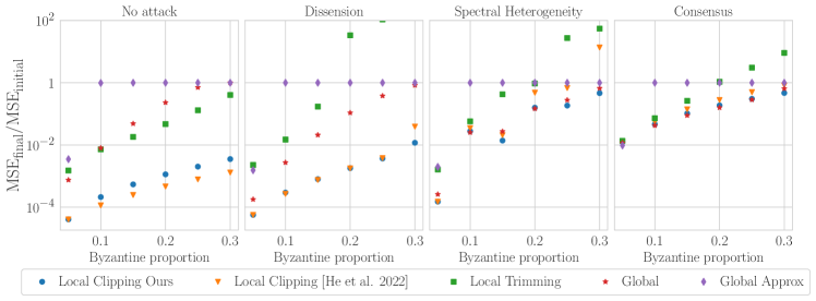
In this section, we provide experiments to support the proposed attacks and robust gossip algorithms. We compare the GCR, the Simplified GCR, the LCR and the local trimming (consistent with NNA proposed in Farhadkhani et al. (2023)) with the rule of thumb Local Clipping proposed in He et al. (2022) which, under the notations of Definition 4.3, consist in taking $\kappa_{j}^{t}=N_{b}(i)+1$. We test these under different attacks. We decompose the parameter sent by a Byzantine neighbor $i$ of an honest node $j$ as $x_{i}^{t}=x_{j}^{t}+\varepsilon_{i}^{t}{\color[rgb]{.75,.5,.25}\definecolor[named]{pgfstrokecolor}{rgb}{.75,.5,.25}u_{i}^{t}}$, where ${\color[rgb]{.75,.5,.25}\definecolor[named]{pgfstrokecolor}{rgb}{.75,.5,.25}u_{i}^{t}}$ is the direction of attack on edge ${(i\sim j)}$ and $\varepsilon_{i}^{t}$ a scaling parameter. Then we implement i) a Consensus attack, in which all Byzantine nodes attack in the same direction: ${\color[rgb]{.75,.5,.25}\definecolor[named]{pgfstrokecolor}{rgb}{.75,.5,.25}u_{i}^{t}}=u$ fixed along time; ii) a No Attack attack where Byzantines take ${\color[rgb]{.75,.5,.25}\definecolor[named]{pgfstrokecolor}{rgb}{.75,.5,.25}u_{i}^{t}}=0$, i.e., they do not influence optimization; iii) the Dissensus attack of He et al. (2022), in which ${\color[rgb]{.75,.5,.25}\definecolor[named]{pgfstrokecolor}{rgb}{.75,.5,.25}u_{i}^{t}}=\sum_{{k\rightarrow j}\in\tilde{\mathcal{E}}_{h}}(x_{j}^{t}-x_{k}^{t})$; iv) our Spectral Heterogeneity attack, in which ${\color[rgb]{.75,.5,.25}\definecolor[named]{pgfstrokecolor}{rgb}{.75,.5,.25}u_{i}^{t}}=[v_{\min}v_{\min}^{T}X_{h}^{t}]_{j:}$. We scale each attack by choosing $\varepsilon_{i}^{t}/\|u_{i}^{t}\|$ to be a) just below the trimming threshold of node $i$ in case of trimming b) arbitrarily large in case of clipping. We perform the experiments on a fully-connected graph, with 20 nodes, and a varying proportion of Byzantine nodes. See Appendix A for experiments on a modified Torus topology. Parameters of honest nodes are independently initialized with a $\mathcal{N}(0,I_{5})$ distribution, and we average the MSE over 200 samples. In Figure 1, we consider the gain of the aggregation scheme on the mean-square error $\mathrm{MSE}_{t}:=\|X_{h}^{t}-\overline{X_{h}^{*}}\|_{F}^{2}$. We stop the aggregation scheme after 30 iterations, which is enough for convergence in absence of disruptions in this case.

6.2 Analysis

Practical performance. On Figure 1, we note that a) In this setting, apart from the proportion of $1/20$ Byzantine nodes (in which local clipping rules are the same), Global Clipping and our Local Clipping outperform Trimming and Local Clipping of He et al. (2022) on the worst-case attack. Yet, Global Clipping has roughly the same performance under all attacks, such that it under-performs under No attack and Dissension attack. b) Spectral Heterogeneity and Consensus attacks significantly outperform the Dissension attack. c) The approximation leading to the Simplified GCR is too loose as it generally leads to a clipping threshold of 00. d) The clipping rule of He et al. (2022) performs better under the No attack attack, which reflects that they under-clip.

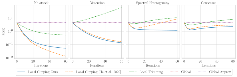
Link with the theory. In Appendix A we displays the decomposition $\mathrm{MSE}\!=\!\mathrm{heterogeneity}\!+\!\mathrm{bias}$ along the gossip process. We remark that Global Clipping ensures monotonicity of the MSE (as predicted by Theorem 3.7), whereas local rules do not: they induce linear convergence of the heterogeneity, but under the price of an additional bias. As such, it supports that we can’t directly prove decreasing of the MSE in local clipping rules, as it is reflected in the proof of Corollary 4.9.

7 Conclusion

We have leveraged the dual approach to design a byzantine-robust decentralized algorithm, and we have analyzed its properties for the average consensus problem under both global and local clipping rules.

Similarly to the fact that different step-size schedules lead to very different behaviors for (S)GD, we argue that the core of (Byzantine-robust) algorithms based on clipping lies on the choice of the clipping threshold. Therefore, while $\operatorname{\operatorname{EdgeClippedGossip}}$ is reminescent of existing algorithms such as $\operatorname{ClippedGossip}$, our clipping rules are novel, practical and theoretically grounded, and they lead to tight convergence results.

8 Impact Statement

This paper presents work whose goal is to advance the field of Machine Learning. There are many potential societal consequences of our work, none which we feel must be specifically highlighted here.

References

  • Alistarh et al. (2018) Alistarh, D., Allen-Zhu, Z., and Li, J. Byzantine stochastic gradient descent. Advances in Neural Information Processing Systems, 31, 2018.
  • Baruch et al. (2019) Baruch, G., Baruch, M., and Goldberg, Y. A little is enough: Circumventing defenses for distributed learning. Advances in Neural Information Processing Systems, 32, 2019.
  • Blanchard et al. (2017) Blanchard, P., El Mhamdi, E. M., Guerraoui, R., and Stainer, J. Machine learning with adversaries: Byzantine tolerant gradient descent. Advances in neural information processing systems, 30, 2017.
  • Boyd et al. (2006) Boyd, S., Ghosh, A., Prabhakar, B., and Shah, D. Randomized gossip algorithms. IEEE transactions on information theory, 52(6):2508–2530, 2006.
  • Chen et al. (2017) Chen, Y., Su, L., and Xu, J. Distributed statistical machine learning in adversarial settings: Byzantine gradient descent. Proceedings of the ACM on Measurement and Analysis of Computing Systems, 1(2):1–25, 2017.
  • Duchi et al. (2011) Duchi, J. C., Agarwal, A., and Wainwright, M. J. Dual averaging for distributed optimization: Convergence analysis and network scaling. IEEE Transactions on Automatic control, 57(3):592–606, 2011.
  • El-Mhamdi et al. (2020) El-Mhamdi, E.-M., Guerraoui, R., Guirguis, A., Hoang, L. N., and Rouault, S. Genuinely distributed byzantine machine learning. In Proceedings of the 39th Symposium on Principles of Distributed Computing, pp.  355–364, 2020.
  • El-Mhamdi et al. (2021) El-Mhamdi, E. M., Farhadkhani, S., Guerraoui, R., Guirguis, A., Hoang, L.-N., and Rouault, S. Collaborative learning in the jungle (decentralized, byzantine, heterogeneous, asynchronous and nonconvex learning). Advances in Neural Information Processing Systems, 34:25044–25057, 2021.
  • Fang et al. (2022) Fang, C., Yang, Z., and Bajwa, W. U. Bridge: Byzantine-resilient decentralized gradient descent. IEEE Transactions on Signal and Information Processing over Networks, 8:610–626, 2022.
  • Farhadkhani et al. (2022) Farhadkhani, S., Guerraoui, R., Gupta, N., Pinot, R., and Stephan, J. Byzantine machine learning made easy by resilient averaging of momentums. In International Conference on Machine Learning, pp. 6246–6283. PMLR, 2022.
  • Farhadkhani et al. (2023) Farhadkhani, S., Guerraoui, R., Gupta, N., Hoang, L.-N., Pinot, R., and Stephan, J. Robust collaborative learning with linear gradient overhead. In International Conference on Machine Learning, pp. 9761–9813. PMLR, 2023.
  • Gorbunov et al. (2022) Gorbunov, E., Borzunov, A., Diskin, M., and Ryabinin, M. Secure distributed training at scale. In International Conference on Machine Learning, pp. 7679–7739. PMLR, 2022.
  • He et al. (2022) He, L., Karimireddy, S. P., and Jaggi, M. Byzantine-robust decentralized learning via clippedgossip. arXiv preprint arXiv:2202.01545, 2022.
  • Hendrikx et al. (2019) Hendrikx, H., Bach, F., and Massoulié, L. Accelerated decentralized optimization with local updates for smooth and strongly convex objectives. In The 22nd International Conference on Artificial Intelligence and Statistics, pp.  897–906. PMLR, 2019.
  • Hendrikx et al. (2020) Hendrikx, H., Bach, F., and Massoulié, L. Dual-free stochastic decentralized optimization with variance reduction. Advances in neural information processing systems, 33:19455–19466, 2020.
  • Hendrikx et al. (2021) Hendrikx, H., Bach, F., and Massoulie, L. An optimal algorithm for decentralized finite-sum optimization. SIAM Journal on Optimization, 31(4):2753–2783, 2021.
  • Jakovetić et al. (2020) Jakovetić, D., Bajović, D., Xavier, J., and Moura, J. M. Primal–dual methods for large-scale and distributed convex optimization and data analytics. Proceedings of the IEEE, 108(11):1923–1938, 2020.
  • Karimireddy et al. (2020) Karimireddy, S. P., He, L., and Jaggi, M. Byzantine-robust learning on heterogeneous datasets via bucketing. arXiv preprint arXiv:2006.09365, 2020.
  • Karimireddy et al. (2021) Karimireddy, S. P., He, L., and Jaggi, M. Learning from history for byzantine robust optimization. In International Conference on Machine Learning, pp. 5311–5319. PMLR, 2021.
  • Kovalev et al. (2020) Kovalev, D., Salim, A., and Richtárik, P. Optimal and practical algorithms for smooth and strongly convex decentralized optimization. Advances in Neural Information Processing Systems, 33:18342–18352, 2020.
  • Kuwaranancharoen & Sundaram (2023) Kuwaranancharoen, K. and Sundaram, S. On the geometric convergence of byzantine-resilient distributed optimization algorithms. arXiv preprint arXiv:2305.10810, 2023.
  • Lamport et al. (1982) Lamport, L., Shostak, R., and Pease, M. The byzantine generals problem. ACM Transactions on Programming Languages and Systems, 4(3):382–401, 1982.
  • LeBlanc et al. (2013) LeBlanc, H. J., Zhang, H., Koutsoukos, X., and Sundaram, S. Resilient asymptotic consensus in robust networks. IEEE Journal on Selected Areas in Communications, 31(4):766–781, 2013.
  • Li et al. (2019) Li, L., Xu, W., Chen, T., Giannakis, G. B., and Ling, Q. Rsa: Byzantine-robust stochastic aggregation methods for distributed learning from heterogeneous datasets. In Proceedings of the AAAI Conference on Artificial Intelligence, volume 33, pp.  1544–1551, 2019.
  • Nedic & Ozdaglar (2009) Nedic, A. and Ozdaglar, A. Distributed subgradient methods for multi-agent optimization. IEEE Transactions on Automatic Control, 54(1):48–61, 2009.
  • Peng et al. (2021) Peng, J., Li, W., and Ling, Q. Byzantine-robust decentralized stochastic optimization over static and time-varying networks. Signal Processing, 183:108020, 2021.
  • Scaman et al. (2017) Scaman, K., Bach, F., Bubeck, S., Lee, Y. T., and Massoulié, L. Optimal algorithms for smooth and strongly convex distributed optimization in networks. In international conference on machine learning, pp. 3027–3036. PMLR, 2017.
  • Uribe et al. (2020) Uribe, C. A., Lee, S., Gasnikov, A., and Nedić, A. A dual approach for optimal algorithms in distributed optimization over networks. In 2020 Information Theory and Applications Workshop (ITA), pp.  1–37. IEEE, 2020.
  • Vaidya (2014) Vaidya, N. H. Iterative byzantine vector consensus in incomplete graphs. In Distributed Computing and Networking: 15th International Conference, ICDCN 2014, Coimbatore, India, January 4-7, 2014. Proceedings 15, pp.  14–28. Springer, 2014.
  • Vaidya et al. (2012) Vaidya, N. H., Tseng, L., and Liang, G. Iterative approximate byzantine consensus in arbitrary directed graphs. In Proceedings of the 2012 ACM symposium on Principles of distributed computing, pp.  365–374, 2012.
  • Wu et al. (2023) Wu, Z., Chen, T., and Ling, Q. Byzantine-resilient decentralized stochastic optimization with robust aggregation rules. IEEE transactions on signal processing, 2023.
  • Xie et al. (2020) Xie, C., Koyejo, O., and Gupta, I. Fall of empires: Breaking byzantine-tolerant sgd by inner product manipulation. In Uncertainty in Artificial Intelligence, pp.  261–270. PMLR, 2020.
  • Yin et al. (2018) Yin, D., Chen, Y., Kannan, R., and Bartlett, P. Byzantine-robust distributed learning: Towards optimal statistical rates. In International Conference on Machine Learning, pp. 5650–5659. PMLR, 2018.

In this Appendix, we provide some complementary elements on the content on the paper. In particular, in Appendix B, we provide proofs of the results given in the paper.

Appendix A Additional experiments

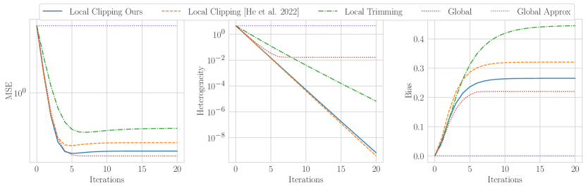
Heterogeneity/bias decomposition. In Figure 2 we display the evolution of the mean-square error (MSE) $\|X_{h}^{t}-\overline{X_{h}^{*}}\|_{F}^{2}$, of the heterogeneity $\|X_{h}^{t}-\overline{X_{h}^{t}}\|_{F}$ and of the bias $|\overline{X_{h}^{t}}-\overline{X_{h}^{*}}|$ along the communication process with in a fully-connected graph with $\frac{1}{9}$ of Byzantine neighbors under a Consensus attack. We see that all aggregation rules are robust in this setting, and that the Global Clipping rule performs the best even if it does not allows to reach consensus. We note that for local aggregation rules the MSE is not monotone, as an additional bias is paid for reaching consensus. Hence the consensus is achieved under the price of this bias. This raises the question of the relevance of seeking only decentralized communication algorithm that aims at reaching asymptotic consensus, as allowing approximate agreement can be a way to reduce the bias. Note that we displayed here only the Consensus attack, but the conclusion would be the same for the other attacks described in Section 6.

Refer to caption

Figure 2: Consensus attack in a fully-connected graph with 16 honest and 2 Byzantine nodes.

Sparse graph. We consider now a modified Torus topology, with one additional honest node connected with everyone. Hence, in this graph, each honest node is connected to 5 other honest nodes, apart from one which is connected to every other honest nodes. In Figure 3 we test all attacks in this Torus topology, with 15 honest nodes in the Torus, one honest principal nodes, and 2 Byzantine neighbors per honest node. In this setting $\Delta_{\infty}\approx 1.5$, such that the Global Clipping rules enforce no communication. In this setting SP attack is the only one that disrupt the Local Clipping strategy of (He et al., 2022).

Refer to caption

Figure 3: Different attacks in a Torus topology with an additionnal honest principal node. The graph is composed of 16 honest nodes, each having 2 Byzantine neighbors.

Appendix B Proofs

B.1 Proof of Global Clipping Rule (GCR) Theorem 3.7

B.1.1 Notations

In this subsection we resume the different notations of the proofs.

We recall the algorithm in the global clipping setting:

$\displaystyle X_{h}^{t+1}$ $\displaystyle=X_{h}^{t}-\eta(C_{h}\,C_{b})\operatorname{Clip}(C^{T}X^{t};\boldsymbol{\tau}^{t})$
$\displaystyle X_{b}^{t+1}$ $\displaystyle=*.$

In the global clipping setting, we consider that, as $\boldsymbol{\tau}^{t}=\tau^{t}\textbf{1}_{\mathcal{E}}$, we can overload the clipping operators writing for $\Lambda_{h}\in\mathbb{R}^{\mathcal{E}_{h}\times d}$ and $\Lambda_{b}\in\mathbb{R}^{\mathcal{E}_{b}\times d}$,

$\displaystyle\operatorname{Clip}(\Lambda_{h};\tau^{t})=[\operatorname{Clip}(\lambda_{{(i\sim j)}},\tau^{t})]_{{(i\sim j)}\in\mathcal{E}_{h}}$ (19)
$\displaystyle\operatorname{Clip}(\Lambda_{b};\tau^{t})=[\operatorname{Clip}(\lambda_{{(i\sim j)}},\tau^{t})]_{{(i\sim j)}\in\mathcal{E}_{b}}$ (20)

We use the following notations:

  • For any matrix $M\in\mathbb{R}^{\mathcal{V}_{h}\times d}$, we denote

    $$\overline{M}:=\frac{1}{n_{h}}\textbf{1}_{n_{h}}\textbf{1}_{n_{h}}^{T}M.$$
  • We note the primal parameter re-centered on the solution

    $$Z_{h}^{t}:=X_{h}^{t}-\overline{X^{*}_{h}}.$$
  • The unitary matrix of attacks directions on Byzantine edge

    $$U_{b}^{t}:=\frac{1}{\eta\tau^{t}}(\Lambda_{b}^{t+1}-\Lambda_{b}^{t}).$$

    Thus $\|U_{b}^{t}\|_{\infty,2}\leqslant 1$ and $\Lambda_{b}^{t+1}=\Lambda_{b}^{t}-\eta\operatorname{Clip}([C^{T}X^{t}]_{b};\tau^{t})=\Lambda_{b}^{t}+\eta\tau^{t}U_{b}^{t}$.

  • The error term induced by clipping and Byzantine nodes

    $$E^{t}:=C_{h}\left(C_{h}^{T}Z^{t}_{h}-\operatorname{Clip}(C_{h}^{T}Z^{t}_{h};\tau^{t})\right)+\tau^{t}C_{b}U_{b}^{t},$$
  • We denote for $p\in\{1,2\}$ and $\kappa^{t}\in\{0,\ldots,|\mathcal{E}_{h}|\}$

    $\displaystyle\|C_{h}^{T}X_{h}^{t}\|_{p;{\kappa^{t}}}^{p}:=$ $\displaystyle\sum_{\begin{subarray}{c}{(i\sim j)}\in\mathcal{E}_{h},\ \ \kappa^{t}\text{ largest}\end{subarray}}\|(C_{h}^{T}X_{h}^{t})_{{(i\sim j)}}\|_{2}^{p}$
    $\displaystyle\|C_{h}^{T}X_{h}^{t}\|_{p;{-\kappa^{t}}}^{p}:=$ $\displaystyle\|C_{h}^{T}X_{h}^{t}\|_{p}^{p}-\|C_{h}^{T}X_{h}^{t}\|_{p;\kappa^{t}}^{p}.$
  • We recall that by default $\|\cdot\|$ and $\|\cdot\|_{2}$ is the usual Euclidean norm (or the Frobenius norm in case of matrix).

And we recall some previous facts:

  • $L_{h}=C_{h}C_{h}^{T}=\frac{1}{2}\tilde{C}_{h}\tilde{C}_{h}^{T}$ the Lagrangian matrix on the honest subgraph $\mathcal{G}_{h}$.

  • $C_{h}^{T}\textbf{1}_{n_{h}}=0\implies C_{h}^{T}\overline{X^{t}_{h}}=0\implies C_{h}^{T}X_{h}^{t}=C_{h}^{T}Z_{h}^{t}$ .

  • $C_{h}^{\dagger}$ is the Moore-Penrose pseudo inverse of $C_{h}$.

B.1.2 Analysis of Global Clipping Rule (GCR) Theorem 3.7

Lemma B.1.

(Gossip - Error decomposition) The iterate update can be decomposed as

$$Z^{t+1}_{h}=(I_{h}-\eta L_{h})Z_{h}^{t}+\eta E^{t}.$$
Proof.

The actualization of $X_{h}^{t}$ writes

$\displaystyle X^{t+1}_{h}$ $\displaystyle=X_{h}^{t}-\eta C_{h}\operatorname{Clip}(C_{h}^{T}X^{t}_{h};\tau^{t})-\eta C_{b}\operatorname{Clip}([C^{T}X^{t}]_{b};\tau^{t}).$

Using $C_{h}^{T}X_{h}^{t}=C_{h}^{T}Z_{h}^{t}$, we get

$\displaystyle Z^{t+1}_{h}$ $\displaystyle=Z_{h}^{t}-\eta C_{h}\operatorname{Clip}(C_{h}^{T}X^{t}_{h};\tau^{t})+\eta\tau^{t}C_{b}U_{b}^{t}$
$\displaystyle=(I_{h}-\eta C_{h}C_{h}^{T})Z_{h}^{t}+\eta\left\{C_{h}\left(C_{h}^{T}Z^{t}_{h}-\operatorname{Clip}(C_{h}^{T}Z^{t}_{h};\tau^{t})\right)+\tau^{t}C_{b}U_{b}^{t}\right\}$
$\displaystyle=(I_{h}-\eta L_{h})Z_{h}^{t}+\eta E^{t}.$

Lemma B.2.

(Sufficient decrease on the variance) We have the decomposition of the variance as a biased gradient descent:

$$\|Z^{t+1}_{h}-\overline{Z_{h}^{t}}\|^{2}=\|Z_{h}^{t}-\overline{Z_{h}^{t}}\|^{2}+\eta^{2}\|L_{h}Z_{h}^{t}-E^{t}\|^{2}-2\eta\|C_{h}^{T}Z_{h}^{t}\|^{2}+2\eta\langle Z_{h}^{t}-\overline{Z_{h}^{t}},E^{t}\rangle.$$
Proof.

we start from Lemma B.1

$\displaystyle\|Z^{t+1}_{h}-\overline{Z^{t}_{h}}\|^{2}$ $\displaystyle=\|Z^{t}_{h}-\overline{Z^{t}_{h}}-\eta(L_{h}Z_{h}^{t}-E^{t})\|^{2}$
$\displaystyle=\|Z^{t}_{h}-\overline{Z^{t}_{h}}\|^{2}+\eta^{2}\|L_{h}Z_{h}^{t}-E^{t}\|^{2}-2\eta\langle L_{h}Z_{h}^{t},Z_{h}^{t}-\overline{Z^{t}_{h}}\rangle+2\eta\langle Z_{h}^{t}-\overline{Z^{t}_{h}},E^{t}\rangle$
$\displaystyle=\|Z^{t}_{h}-\overline{Z^{t}_{h}}\|^{2}+\eta^{2}\|L_{h}Z_{h}^{t}-E^{t}\|^{2}-2\eta\|C_{h}^{T}Z_{h}^{t}\|^{2}+2\eta\langle Z_{h}^{t}-\overline{Z^{t}_{h}},E^{t}\rangle,$

where we used that $C_{h}^{T}\overline{Z_{h}^{t}}=0\text{ and }C_{h}C_{h}^{T}=L_{h}.$

Lemma B.3.

(complete sufficient decrease)

$$\|Z^{t+1}_{h}\|^{2}=\|Z_{h}^{t}\|^{2}+\eta^{2}\|L_{h}Z_{h}^{t}-E^{t}\|^{2}-2\eta\|C_{h}^{T}Z_{h}^{t}\|^{2}+2\eta\langle Z_{h}^{t}-\overline{Z_{h}^{t}},E^{t}\rangle+2\langle\overline{Z^{t}_{h}},\overline{Z^{t+1}_{h}}-\overline{Z^{t}_{h}}\rangle.$$
Proof.

We leverage that

$\displaystyle\|Z^{t+1}_{h}\|^{2}$ $\displaystyle=\|Z^{t+1}_{h}-\overline{Z^{t}_{h}}+\overline{Z^{t}_{h}}\|^{2}$
$\displaystyle=\|Z^{t+1}_{h}-\overline{Z^{t}_{h}}\|^{2}+\|\overline{Z^{t}_{h}}\|^{2}+2\langle\overline{Z^{t}_{h}},Z^{t+1}_{h}-\overline{Z^{t}_{h}}\rangle$
$\displaystyle=\|Z^{t+1}_{h}-\overline{Z^{t}_{h}}\|^{2}+\|\overline{Z^{t}_{h}}\|^{2}+2\langle\overline{Z^{t}_{h}},\overline{Z^{t+1}_{h}}-\overline{Z^{t}_{h}}\rangle.$

Then we use Lemma B.2. ∎

Assumption B.4.

Definition 3.3 Trade-off between clipping error and Byzantine influence. By denoting

$$\Delta_{\infty}:=\sup_{\begin{subarray}{c}U_{b}\in\mathbb{R}^{\mathcal{E}_{b}\times d}\\ \|U_{b}\|_{\infty,2}\leqslant 1\end{subarray}}\|C_{h}^{\dagger}C_{b}U_{b}\|_{\infty,2},$$

We assume that $\tau^{t}=0$, or

$$\|C_{h}^{T}X^{t}_{h}\|_{\kappa^{t}}\geqslant\Delta_{\infty}\|C_{h}^{T}X^{t}_{h}\|_{1}+\eta\frac{|\mathcal{E}_{b}|^{2}}{n_{h}}\sum_{0\leqslant s\leqslant t}\tau^{s}.$$
Lemma B.5.

(Join control of the first order error and second order bias) Under Definition 3.3, we have that

$$\eta\langle Z_{h}^{t}-\overline{Z^{t}_{h}},E^{t}\rangle+\langle\overline{Z^{t}_{h}},\overline{Z^{t+1}_{h}}-\overline{Z^{t}_{h}}\rangle+\eta^{2}\|\overline{E^{t}}\|_{2}^{2}\leqslant\eta\|C_{h}^{T}Z_{h}^{t}\|^{2}_{\kappa^{t}},$$

or $\tau^{t}=0$.

Proof.

We begin by upper bounding precisely both error terms:

  1. 1.

    Variance-induced error.

    $\displaystyle\langle Z_{h}^{t}-\overline{Z^{t}_{h}},E^{t}\rangle$ $\displaystyle=\langle Z_{h}^{t}-\overline{Z^{t}_{h}},C_{h}\left(C_{h}^{T}Z_{h}^{t}-\operatorname{Clip}(C_{h}^{T}Z_{h}^{t};\tau^{t})\right)\rangle+\langle Z_{h}^{t}-\overline{Z^{t}_{h}},\tau^{t}C_{b}U_{b}^{t}\rangle$
    $\displaystyle=\langle C_{h}^{T}Z_{h}^{t},C_{h}^{T}Z_{h}^{t}-\operatorname{Clip}(C_{h}^{T}Z_{h}^{t};\tau^{t})\rangle+\langle C_{h}^{T}Z_{h}^{t},\tau^{t}C_{h}^{\dagger}C_{b}U_{b}^{t}\rangle.$ $\displaystyle\text{ Using that }C_{h}^{T}\overline{Z_{h}^{t}}=0.$

    On one side we have that,

    $$\langle C_{h}^{T}Z_{h}^{t},C_{h}^{T}Z_{h}^{t}-\operatorname{Clip}(C_{h}^{T}Z_{h}^{t};\tau^{t})\rangle=\sum_{{(i\sim j)}\in\mathcal{E}_{h}}\langle z_{i}^{t}-z_{j}^{t},z_{i}^{t}-z_{j}^{t}-\operatorname{Clip}(z_{i}^{t}-z_{j}^{t};\tau^{t})\rangle=\sum_{{(i\sim j)}\in\mathcal{E}_{h}}\|z_{i}^{t}-z_{j}^{t}\|_{2}\left(\|z_{i}^{t}-z_{j}^{t}\|_{2}-\tau^{t}\right)_{+}.$$

    One the other side, by using that, for $M,N\in\mathbb{R}^{\mathcal{E}_{h}\times d}$, $\langle M,N\rangle\leqslant\|M\|_{1,2}\|N\|_{\infty,2}$, as:

    $\displaystyle\langle M,N\rangle$ $\displaystyle=\sum_{{(i\sim j)}\in\mathcal{E}_{h}}\langle M_{{(i\sim j)}},N_{{(i\sim j)}}\rangle$
    $\displaystyle\leqslant\sum_{{(i\sim j)}\in\mathcal{E}_{h}}\|M_{{(i\sim j)}}\|_{2}\|N_{{(i\sim j)}}\|_{2}$
    $\displaystyle\leqslant\|N\|_{\infty,2}\sum_{{(i\sim j)}\in\mathcal{E}_{h}}\|M_{{(i\sim j)}}\|_{2},$

    we can upper bound the second term

    $$\langle C_{h}^{T}Z_{h}^{t},\tau^{t}C_{h}^{\dagger}C_{b}U_{b}^{t}\rangle\leqslant\tau^{t}\|C_{h}^{T}Z_{h}^{T}\|_{1,2}\|C_{h}^{\dagger}C_{b}U_{b}^{t}\|_{\infty,2}.$$

    Then by defining $\Delta_{\infty}=\sup_{U_{b}\in\mathbb{R}^{\mathcal{E}_{b}\times d}}\|C_{h}^{\dagger}C_{b}U_{b}^{t}\|_{\infty,2}$, using $\|C_{h}^{T}Z_{h}^{t}\|_{1,2}=\sum_{{(i\sim j)}\in\mathcal{E}_{h}}\|z_{i}^{t}-z_{j}^{t}\|_{2}$, we have that

    $\displaystyle\langle Z_{h}^{t}-\overline{Z^{t}_{h}},E^{t}\rangle$ $\displaystyle\leqslant\sum_{{(i\sim j)}\in\mathcal{E}_{h}}\|z_{i}^{t}-z_{j}^{t}\|_{2}\left(\|z_{i}^{t}-z_{j}^{t}\|_{2}-\tau^{t}\right)_{+}+\tau^{t}\Delta_{\infty}\sum_{{(i\sim j)}\in\mathcal{E}_{h}}\|z_{i}^{t}-z_{j}^{t}\|_{2}$
    $\displaystyle=\sum_{{(i\sim j)}\in\mathcal{E}_{h}}\|z_{i}^{t}-z_{j}^{t}\|_{2}^{2}\mathds{1}_{\|z_{i}^{t}-z_{j}^{t}\|_{2}>\tau^{t}}-\tau^{t}\left(\sum_{{(i\sim j)}\in\mathcal{E}_{h}}\|z_{i}^{t}-z_{j}^{t}\|_{2}\mathds{1}_{\|z_{i}^{t}-z_{j}^{t}\|_{2}>\tau^{t}}-\Delta_{\infty}\sum_{{(i\sim j)}\in\mathcal{E}_{h}}\|z_{i}^{t}-z_{j}^{t}\|_{2}^{2}\right).$

    Let’s consider any $\kappa^{t}\in\mathbb{N}$ such that

    $$\kappa^{t}\in\left[\sum_{{(i\sim j)}\in\mathcal{E}_{h}}\mathds{1}_{\|z_{i}^{t}-z_{j}^{t}\|_{2}>\tau^{t}},\sum_{{(i\sim j)}\in\mathcal{E}_{h}}\mathds{1}_{\|z_{i}^{t}-z_{j}^{t}\|_{2}\geqslant\tau^{t}}-1\right].$$

    Then, using

    $$\|C_{h}^{T}Z_{h}^{t}\|_{p,\kappa^{t}}^{p}:=\sum_{\begin{subarray}{c}{(i\sim j)}\in\mathcal{E}_{h}\\ \kappa^{t}\text{ largest}\end{subarray}}\|z_{i}^{t}-z_{j}^{t}\|_{2}^{p},$$

    the previous inequality writes

    $$\langle Z_{h}^{t}-\overline{Z^{t}_{h}},E^{t}\rangle\leqslant\|C_{h}^{T}Z_{h}^{t}\|_{2,\kappa^{t}}^{2}-\tau^{t}\left(\|C_{h}^{T}Z_{h}^{t}\|_{1,\kappa^{t}}-\Delta_{\infty}\|C_{h}^{T}Z_{h}^{t}\|_{1}\right).$$

    From this upper bound we could derive a clipping rule taking only into account the error induced by clipping and Byzantine nodes on the variance. In this analysis, we will include the second error term induced by the bias.

  2. 2.

    Bias-induced error.
    We consider the term $\langle\overline{Z_{h}^{t}},\overline{Z_{h}^{t+1}}-\overline{Z_{h}^{t}}\rangle$. We remark that, using that $Z^{t+1}_{h}=(I_{h}-C_{h}C_{h}^{T})Z^{t}_{h}+\eta E^{t}$, and considering that $\textbf{1}_{n_{h}}^{T}C_{h}=0$, using the definition of $E^{t}$ we get:

    $$\textbf{1}_{n_{h}}^{T}Z_{h}^{t+1}=\textbf{1}_{n_{h}}^{T}Z_{h}^{t}+\eta\tau^{t}\textbf{1}_{n_{h}}^{T}C_{b}U_{b}^{t}=\sum_{s=0}^{t}\eta\tau^{s}\textbf{1}_{n_{h}}^{T}C_{b}U_{b}^{s}.$$

    Using this, we remark that

    $$\eta^{2}\|\overline{E^{t}}\|_{2}^{2}=\|\overline{Z^{t+1}}-\overline{Z^{t}}\|_{2}^{2}\implies\eta^{2}\|\overline{E^{t}}\|_{2}^{2}+\langle\overline{Z_{h}^{t}},\overline{Z_{h}^{t+1}}-\overline{Z_{h}^{t}}\rangle=\langle\overline{Z_{h}^{t+1}},\overline{Z_{h}^{t+1}}-\overline{Z_{h}^{t}}\rangle.$$

    Thus we get

    $\displaystyle\langle\overline{Z_{h}^{t+1}},\overline{Z_{h}^{t+1}}-\overline{Z_{h}^{t}}\rangle$ $\displaystyle=\left\langle\sum_{s=0}^{t}\eta\tau^{s}\frac{1}{n_{h}}\textbf{1}_{n_{h}}\textbf{1}_{n_{h}}^{T}C_{b}U_{b}^{s},\eta\tau^{t}\frac{1}{n_{h}}\textbf{1}_{n_{h}}\textbf{1}_{n_{h}}^{T}C_{b}U_{b}^{t}\right\rangle$
    $\displaystyle=\frac{\tau^{t}\eta^{2}}{n_{h}}\sum_{s=0}^{t}\tau^{s}\left\langle\textbf{1}_{n_{h}}^{T}C_{b}U_{b}^{s},\textbf{1}_{n_{h}}^{T}C_{b}U_{b}^{t}\right\rangle$
    $\displaystyle=\frac{\tau^{t}\eta^{2}}{n_{h}}\sum_{s=0}^{t}\tau^{s}\left\langle\sum_{i\in\mathcal{V}_{h}}N_{b}(i)u_{i}^{s},\sum_{i\in\mathcal{V}_{h}}N_{b}(i)u_{i}^{t}\right\rangle.$

    Where $u_{i}^{t}$ is the mean vector of Byzantine neighbors of node $i\in\mathcal{V}_{h}$, so that $\|u_{i}^{t}\|_{2}\leqslant 1$, thus we get

    $\displaystyle\langle\overline{Z_{h}^{t}},\overline{Z_{h}^{t+1}}-\overline{Z_{h}^{t}}\rangle$ $\displaystyle\leqslant\frac{\tau^{t}\eta^{2}}{n_{h}}\sum_{s=0}^{t}\tau^{s}\left(\sum_{i\in\mathcal{V}_{h}}N_{b}(i)\right)^{2}=\frac{\eta^{2}\tau^{t}|\mathcal{E}_{b}|^{2}}{n_{h}}\sum_{s=0}^{t}\tau^{s}.$

Now that we controlled both terms, we can mix both error terms:

$\displaystyle\langle Z_{h}^{t}-\overline{Z^{t}_{h}},E^{t}\rangle+\eta^{-1}\langle\overline{Z^{t}_{h}},\overline{Z^{t+1}_{h}}-\overline{Z^{t}_{h}}\rangle$ $\displaystyle\leqslant\|C_{h}^{T}Z_{h}^{t}\|_{2,\kappa^{t}}^{2}-\tau^{t}\left(\|C_{h}^{T}Z_{h}^{t}\|_{1,\kappa^{t}}-\Delta_{\infty}\|C_{h}^{T}Z_{h}^{t}\|_{1}\right)+\tau^{t}\frac{\eta|\mathcal{E}_{b}|^{2}}{n_{h}}\sum_{s=0}^{t-1}\tau^{s}$
$\displaystyle=\|C_{h}^{T}Z_{h}^{t}\|_{2,\kappa^{t}}^{2}-\tau^{t}\left(\|C_{h}^{T}Z_{h}^{t}\|_{1,\kappa^{t}}-\Delta_{\infty}\|C_{h}^{T}Z_{h}^{t}\|_{1}-\frac{\eta|\mathcal{E}_{b}|^{2}}{n_{h}}\sum_{s=0}^{t}\tau^{s}\right).$

Hence, as long as

$$\|C_{h}^{T}Z_{h}^{t}\|_{1,\kappa^{t}}\geqslant\Delta_{\infty}\|C_{h}^{T}Z_{h}^{t}\|_{1}+\frac{\eta|\mathcal{E}_{b}|^{2}}{n_{h}}\sum_{s=0}^{t}\tau^{s},$$ (21)

we have that

$$\langle Z_{h}^{t}-\overline{Z^{t}_{h}},E^{t}\rangle+\eta^{-1}\langle\overline{Z^{t+1}_{h}},\overline{Z^{t+1}_{h}}-\overline{Z^{t}_{h}}\rangle\leqslant\|C_{h}^{T}Z_{h}^{t}\|^{2}_{2,\kappa^{t}}.$$

When Equation 21 cannot be enforced using $\kappa^{t}\leqslant|\mathcal{E}_{h}|-1$, then we take $\tau^{t}=0$ (thus $\kappa^{t}=|\mathcal{E}_{h}|$), everything is clipped and nodes parameters don’t move anymore. ∎

Lemma B.6.

(Control of first and 2nd order error terms together) Assume Definition 3.3 and that

$$\eta\leqslant\frac{1}{\mu_{\max}(L_{h})},$$

then by denoting the first and 2nd order error term, divided by $\eta$ as

$$\zeta^{t}:=\eta\|L_{h}Z_{h}^{t}-E^{t}\|^{2}+2\langle Z_{h}^{t}-\overline{Z_{h}^{t}},E^{t}\rangle+2\eta^{-1}\langle\overline{Z^{t}_{h}},\overline{Z^{t+1}_{h}}-\overline{Z^{t}_{h}}\rangle.$$

We have the control:

$$\zeta^{t}\leqslant\eta\mu_{\max}(L_{h})\left(\|C_{h}^{T}Z_{h}^{t}\|^{2}_{2,-\kappa^{t}}+(\tau^{t})^{2}\left[\kappa^{t}(1-2\Delta_{\infty})+\Delta_{\infty}^{2}|\mathcal{E}_{h}|\right]\right)+2\|C_{h}^{T}Z_{h}^{t}\|_{2,\kappa^{t}}^{2}.$$
Proof.

This part of the proof allows to compute the maximum stepsize usable. We want to control the discretization term $\eta^{2}\|L_{h}Z_{h}^{t}-E^{t}\|^{2}_{2}$. If $E^{t}=0$ it would have been done using a step-size small enough. In this case we will do the same, but we will monitor the interactions between the discretization and the control of the error. Note that

$$E^{t}-L_{h}Z_{h}^{t}=C_{h}\operatorname{Clip}(C_{h}^{T}Z_{h}^{t};\tau^{t})+\tau^{t}C_{b}U_{b}^{t},$$ (22)

and that at the first order $\langle C_{g}\operatorname{Clip}(C_{g}^{T}Z_{h}^{t};\tau^{t}),\tau^{t}C_{b}U_{b}^{t}\rangle\leqslant 0$ if Byzantine aims at preventing the convergence. Thus, we will include this second-order term in the proof of the Lemma B.2.

We denote by $\mu_{\max}(L_{h})$ the largest eigenvalue of $L_{h}$.

We denote the first and 2nd order error term, divided by $\eta$ as

$$\zeta^{t}:=\eta\|L_{h}Z_{h}^{t}-E^{t}\|^{2}+2\langle Z_{h}^{t}-\overline{Z_{h}^{t}},E^{t}\rangle+2\eta^{-1}\langle\overline{Z^{t}_{h}},\overline{Z^{t+1}_{h}}-\overline{Z^{t}_{h}}\rangle.$$

Hence $\|Z_{h}^{t+1}\|^{2}\leqslant\|Z_{h}^{t}\|^{2}+\eta\zeta^{t}-2\eta\|C_{h}^{T}Z_{h}^{t}\|^{2}.$

Using

$$\|E^{t}-L_{h}Z_{h}^{t}\|=\|C_{h}(\operatorname{Clip}(C_{h}^{T}Z_{h}^{t};\tau^{t})-\tau^{t}C_{h}^{\dagger}C_{b}U_{b}^{t})+\overline{E^{t}}\|^{2}=\|C_{h}(\operatorname{Clip}(C_{h}^{T}Z_{h}^{t};\tau^{t})-\tau^{t}C_{h}^{\dagger}C_{b}U_{b}^{t})\|^{2}+\|\overline{E^{t}}\|^{2},$$

we have:

$\displaystyle\zeta^{t}$ $\displaystyle=\eta\|C_{h}(\operatorname{Clip}(C_{h}^{T}Z_{h}^{t};\tau^{t})-\tau^{t}C_{h}^{\dagger}C_{b}U_{b}^{t})\|^{2}_{2}+\eta\|\overline{E^{t}}\|_{2}^{2}$
$\displaystyle+2\langle Z_{h}^{t}-\overline{Z_{h}^{t}},E^{t}\rangle+2\eta^{-1}\langle\overline{Z^{t}_{h}},\overline{Z^{t+1}_{h}}-\overline{Z^{t}_{h}}\rangle$
$\displaystyle\leqslant\eta\mu_{\max}(L_{h})\left(\|\operatorname{Clip}(C_{h}^{T}Z_{h}^{t};\tau^{t})\|^{2}+\|\tau^{t}C_{h}^{\dagger}C_{b}U_{b}^{t}\|^{2}\right)-2\eta\mu_{\max}(L_{h})\langle\operatorname{Clip}(C_{h}^{T}Z_{h}^{t})-C_{h}^{T}Z_{h}^{t}+C_{h}^{T}Z_{h}^{t},\tau^{t}C_{h}^{\dagger}C_{b}U_{b}^{t}\rangle$
$\displaystyle+2\langle C_{h}^{T}Z_{h}^{t},\tau^{t}C_{h}^{\dagger}C_{b}U_{b}^{t}\rangle+2\langle C_{h}^{T}Z_{h}^{t},C_{h}^{T}Z_{h}^{t}-\operatorname{Clip}(C_{h}^{T}Z_{h}^{t};\tau^{t})\rangle+2\eta^{-1}\langle\overline{Z^{t+1}_{h}},\overline{Z^{t+1}_{h}}-\overline{Z^{t}_{h}}\rangle$
$\displaystyle=\eta\mu_{\max}(L_{h})\left(\|\operatorname{Clip}(C_{h}^{T}Z_{h}^{t};\tau^{t})\|^{2}+\|\tau^{t}C_{h}^{\dagger}C_{b}U_{b}^{t}\|^{2}\right)$
$\displaystyle+2\langle C_{h}^{T}Z_{h}^{t},C_{h}^{T}Z_{h}^{t}-\operatorname{Clip}(C_{h}^{T}Z_{h}^{t};\tau^{t})\rangle+2\eta^{-1}\langle\overline{Z^{t+1}_{h}},\overline{Z^{t+1}_{h}}-\overline{Z^{t}_{h}}\rangle$
$\displaystyle+2(1-\eta\mu_{\max}(L_{h}))\underbrace{\langle C_{h}^{T}Z_{h}^{t},\tau^{t}C_{h}^{\dagger}C_{b}U_{b}^{t}\rangle}_{\leqslant\|C_{h}^{T}Z_{h}^{t}\|_{1}\Delta_{\infty}\tau^{t}}+2\eta\mu_{\max}(L_{h})\underbrace{\langle C_{h}^{T}Z_{h}^{t}-\operatorname{Clip}(C_{h}^{T}Z_{h}^{t};\tau^{t}),\tau^{t}C_{h}^{\dagger}C_{b}U_{b}^{t}\rangle}_{{\leqslant\|C_{h}^{T}Z_{h}^{t}-\operatorname{Clip}(C_{h}^{T}Z_{h}^{t};\tau^{t})\|_{1}\Delta_{\infty}\tau^{t}}}.$

Then we use that

$$\|C_{h}^{T}Z_{h}^{t}-\operatorname{Clip}(C_{h}^{T}Z_{h}^{t};\tau^{t})\|_{1}=\|C_{h}^{T}Z_{h}^{t}\|_{1}-\|\operatorname{Clip}(C_{h}^{T}Z_{h}^{t};\tau^{t})\|_{1},$$

to get, for $\eta\leqslant\mu_{\max}(L_{h})$,

$\displaystyle\zeta^{t}$ $\displaystyle\leqslant\eta\mu_{\max}(L_{h})\left(\|\operatorname{Clip}(C_{h}^{T}Z_{h}^{t};\tau^{t})\|^{2}+\|\tau^{t}C_{h}^{\dagger}C_{b}U_{b}^{t}\|^{2}\right)$
$\displaystyle+2\langle C_{h}^{T}Z_{h}^{t},C_{h}^{T}Z_{h}^{t}-\operatorname{Clip}(C_{h}^{T}Z_{h}^{t};\tau^{t})\rangle+2\eta^{-1}\langle\overline{Z^{t+1}_{h}},\overline{Z^{t+1}_{h}}-\overline{Z^{t}_{h}}\rangle$
$\displaystyle+2(1-\eta\mu_{\max}(L_{h}))\|C_{h}^{T}Z_{h}^{t}\|_{1}\Delta_{\infty}\tau^{t}+2\eta\mu_{\max}(L_{h})\|C_{h}^{T}Z_{h}^{t}\|_{1}\Delta_{\infty}\tau^{t}-2\eta\mu_{\max}(L_{h})\|\operatorname{Clip}(C_{h}^{T}Z_{h}^{t};\tau^{t})\|_{1}\Delta_{\infty}\tau^{t}$
$\displaystyle\leqslant\eta\mu_{\max}(L_{h})\left(\|\operatorname{Clip}(C_{h}^{T}Z_{h}^{t};\tau^{t})\|^{2}+\|\tau^{t}C_{h}^{\dagger}C_{b}U_{b}^{t}\|^{2}-2\|\operatorname{Clip}(C_{h}^{T}Z_{h}^{t};\tau^{t})\|_{1}\Delta_{\infty}\tau^{t}\right)$
$\displaystyle+2\langle C_{h}^{T}Z_{h}^{t},C_{h}^{T}Z_{h}^{t}-\operatorname{Clip}(C_{h}^{T}Z_{h}^{t};\tau^{t})\rangle+2\|C_{h}^{T}Z_{h}^{t}\|_{1}\Delta_{\infty}\tau^{t}+2\eta^{-1}\langle\overline{Z^{t+1}_{h}},\overline{Z^{t+1}_{h}}-\overline{Z^{t}_{h}}.\rangle$

Then, the second term is controlled using the proof of Lemma B.5.

By denoting

$$\Delta_{2}^{2}:=\sup_{\|U_{b}^{t}\|_{\infty,2}\leqslant 1}\|C_{h}^{\dagger}C_{b}U_{b}^{t}\|^{2}_{2},$$

we have that, under Definition 3.3

$\displaystyle\zeta^{t}$ $\displaystyle\leqslant\eta\mu_{\max}(L_{h})\left(\|C_{h}^{T}Z_{h}^{t}\|^{2}_{2,-\kappa^{t}}+\tau^{t}\left(\tau^{t}\kappa^{t}+\tau^{t}\Delta_{2}^{2}-2\tau^{t}\kappa^{t}\Delta_{\infty}-2\Delta_{\infty}\|C_{h}^{T}Z_{h}^{t}\|_{1,-\kappa^{t}}\right)\right)+2\|C_{h}^{T}Z_{h}^{t}\|_{2,\kappa^{t}}^{2}$
$\displaystyle\leqslant\eta\mu_{\max}(L_{h})\left((1-\Delta_{\infty})\|C_{h}^{T}Z_{h}^{t}\|^{2}_{2,-\kappa^{t}}+(\tau^{t})^{2}\left[\kappa^{t}(1-2\Delta_{\infty})+\Delta_{2}^{2}\right]\right)+2\|C_{h}^{T}Z_{h}^{t}\|_{2,\kappa^{t}}^{2}.$

Eventually, leveraging that $\Delta_{2}^{2}\leqslant\Delta_{\infty}^{2}|\mathcal{E}_{h}|$, we have

$$\zeta^{t}\leqslant\eta\mu_{\max}(L_{h})\left(\|C_{h}^{T}Z_{h}^{t}\|^{2}_{2,-\kappa^{t}}+(\tau^{t})^{2}\left[\kappa^{t}(1-2\Delta_{\infty})+\Delta_{\infty}^{2}|\mathcal{E}_{h}|\right]\right)+2\|C_{h}^{T}Z_{h}^{t}\|_{2,\kappa^{t}}^{2}.$$

Theorem B.7.

Hence, under Definition 3.3, for

$$\eta\leqslant\frac{\mu_{\max}(L_{h})^{-1}}{1+|\mathcal{E}_{h}|(1-\Delta_{\infty})},$$

we have

$$\|Z^{t+1}_{h}\|^{2}\leqslant\|Z^{t}_{h}\|^{2}-\eta\|C_{h}^{T}Z^{t}_{h}\|^{2}_{2,-\kappa^{t}}.$$
Proof.

We start from Lemma B.3 and use the majoration of the error from Lemma B.6:

$\displaystyle\|Z^{t+1}_{h}\|^{2}$ $\displaystyle=\|Z_{h}^{t}\|^{2}-2\eta\|C_{h}^{T}Z_{h}^{t}\|^{2}+\eta^{2}\|L_{h}Z_{h}^{t}-E^{t}\|^{2}+2\eta\langle Z_{h}^{t}-\overline{Z_{h}^{t}},E^{t}\rangle+2\langle\overline{Z^{t}_{h}},\overline{Z^{t+1}_{h}}-\overline{Z^{t}_{h}}\rangle$
$\displaystyle\leqslant\|Z_{h}^{t}\|-2\eta\|C_{h}^{T}Z_{h}^{t}\|_{2}^{2}++2\eta\|C_{h}^{T}Z_{h}^{t}\|_{2,\kappa^{t}}^{2}$
$\displaystyle+\eta^{2}\mu_{\max}(L_{h})\left(\|C_{h}^{T}Z_{h}^{t}\|^{2}_{2,-\kappa^{t}}+(\tau^{t})^{2}\left[\kappa^{t}(1-2\Delta_{\infty})+\Delta_{\infty}^{2}|\mathcal{E}_{h}|\right]\right)$
$\displaystyle=\|Z_{h}^{t}\|-2\eta\|C_{h}^{T}Z_{h}^{t}\|^{2}_{2,-\kappa^{t}}$
$\displaystyle+\eta^{2}\mu_{\max}(L_{h})\left(\|C_{h}^{T}Z_{h}^{t}\|^{2}_{2,-\kappa^{t}}+(\tau^{t})^{2}\left[\kappa^{t}(1-2\Delta_{\infty})+\Delta_{\infty}^{2}|\mathcal{E}_{h}|\right]\right)$
$\displaystyle\leqslant\|Z_{h}^{t}\|-\eta\left[2-\eta\mu_{\max}(L_{h})\left(1+\kappa^{t}(1-2\Delta_{\infty})+\Delta_{\infty}^{2}|\mathcal{E}_{h}|\right)\right]\|C_{h}^{T}Z_{h}^{t}\|^{2}_{2,-\kappa^{t}}.$

Where we used that, as $\kappa^{t}\leqslant\sum_{{(i\sim j)}\in\mathcal{E}_{h}}\mathds{1}_{\|z_{i}^{t}-z_{j}^{t}\|\geqslant\tau^{t}}-1$, the largest term in $\|C_{h}^{T}Z_{h}^{t}\|^{2}_{2,-\kappa^{t}}$ is $(\tau^{t})^{2}$.

Hence, for

$$\eta\leqslant\frac{\mu_{\max}(L_{h})^{-1}}{1+\kappa^{t}(1-2\Delta_{\infty})+\Delta_{\infty}^{2}|\mathcal{E}_{h}|},$$

or, using a simpler (and stricter) condition

$$\eta\leqslant\frac{\mu_{\max}(L_{h})^{-1}}{1+|\mathcal{E}_{h}|(1-\Delta_{\infty})},$$

we have

$$\|Z^{t+1}_{h}\|^{2}\leqslant\|Z^{t}_{h}\|^{2}-\eta\|C_{h}^{T}Z^{t}_{h}\|^{2}_{2,-\kappa^{t}}.$$

B.1.3 Computing significant quantities

We recall that

$$\Delta_{\infty}:=\sup_{\begin{subarray}{c}U_{b}\in\mathbb{R}^{\mathcal{E}_{b}\times d}\\ \|U_{b}\|_{\infty,2}\leqslant 1\end{subarray}}\|C_{h}^{\dagger}C_{b}U_{b}\|_{\infty,2}.$$
Proposition B.8.

(Computing $\Delta_{\infty}$) Consider a fully connected graph $\mathcal{G}$, we have that

$$\Delta_{\infty}\leqslant\sup_{{(i\sim j)}\in\mathcal{E}_{h}}\frac{2n_{b}}{n_{h}}\sqrt{d\wedge|\mathcal{E}_{b}|},$$

where $n_{b}$ is the number of Byzantines nodes and $n_{h}$ the number of honest nodes.

Proof.

In a fully connected graph $L_{h}=n_{h}I_{h}-\textbf{1}_{h}\textbf{1}_{h}^{T}$, thus $C_{h}^{\dagger}=C_{h}^{T}L_{h}^{\dagger}=\frac{1}{n_{h}}C_{h}^{T}$. Using this, we compute:

$\displaystyle\Delta_{\infty}$ $\displaystyle=\sup_{\begin{subarray}{c}U_{b}\in\mathbb{R}^{\mathcal{E}_{b}\times d}\\ \|U_{b}\|_{\infty,2}\leqslant 1\end{subarray}}\|C_{h}^{\dagger}C_{b}U_{b}\|_{\infty,2}$
$\displaystyle=\frac{1}{n_{h}}\sup_{\begin{subarray}{c}U_{b}\in\mathbb{R}^{\mathcal{E}_{b}\times d}\\ \|U_{b}\|_{\infty,2}\leqslant 1\end{subarray}}\sup_{{(i\sim j)}\in\mathcal{E}_{h}}\|[C_{h}^{T}C_{b}U_{b}]_{{(i\sim j)},:}\|_{2}.$

For ${(i\sim j)}\in\mathcal{E}_{h},$

$\displaystyle\sup_{\begin{subarray}{c}U_{b}\in\mathbb{R}^{\mathcal{E}_{b}\times d}\\ \|U_{b}\|_{\infty,2}\leqslant 1\end{subarray}}\|[C_{h}^{T}C_{b}U_{b}]_{{(i\sim j)},:}\|_{2}^{2}$ $\displaystyle=\sup_{\begin{subarray}{c}U_{b}\in\mathbb{R}^{\mathcal{E}_{b}\times d}\\ \|U_{b}\|_{\infty,2}\leqslant 1\end{subarray}}\sum_{k=1}^{d}\left([C_{h}^{T}C_{b}]_{{(i\sim j)},:}^{T}[U_{b}]_{:,k}\right)^{2}$
$\displaystyle=\sup_{\begin{subarray}{c}U_{b}\in\mathbb{R}^{\mathcal{E}_{b}\times d}\\ \|U_{b}\|_{\infty,2}\leqslant 1\end{subarray}}\sum_{k=1}^{d}\left([[C_{b}]_{i,:}-[C_{b}]_{j,:}]^{T}[U_{b}]_{:,k}\right)^{2}$
$\displaystyle\leqslant\sup_{\begin{subarray}{c}U_{b}\in\mathbb{R}^{\mathcal{E}_{b}\times d}\\ \|U_{b}\|_{\infty,2}\leqslant 1\end{subarray}}\sum_{k=1}^{d}\|[[C_{b}]_{i,:}-[C_{b}]_{j,:}]\|_{1}^{2}\|[U_{b}]_{:,k}\|_{\infty}^{2}$
$\displaystyle\leqslant(N_{b}(i)+N_{b}(j))^{2}\sup_{\begin{subarray}{c}U_{b}\in\mathbb{R}^{\mathcal{E}_{b}\times d}\\ \|U_{b}\|_{\infty,2}\leqslant 1\end{subarray}}\sum_{k=1}^{d}\|[U_{b}]_{:,k}\|_{\infty}^{2}$
$\displaystyle\leqslant(N_{b}(i)+N_{b}(j))^{2}(d\wedge|\mathcal{E}_{b}|).$

Hence, we get:

$$\Delta_{\infty}\leqslant\sup_{{(i\sim j)}\in\mathcal{E}_{h}}\frac{N_{b}(i)+N_{b}(j)}{n_{h}}\sqrt{d\wedge|\mathcal{E}_{b}|}.$$

Thus, assuming that, as we are in a fully-connected graph, every honest node is connected to $n_{b}$ Byzantine node, we get the result

Proposition B.9 (Simplified GCR).

If $(\tau^{t})_{t\geqslant 0}$ is such that: for all $t\geqslant 0$, either $\tau^{t}=0$ or

$$\kappa^{t}\geqslant\Delta_{\infty}|\mathcal{E}_{h}|+\eta\frac{|\mathcal{E}_{b}|^{2}}{{n_{h}}}\sum_{s\leqslant t}\frac{\tau^{s}}{\tau^{t}},$$ (23)

then $(\tau^{s})_{s\geqslant 0}$ satisfies the GCR.

Proof.

(GCR), i.e Equation 21 writes

$$\|C_{h}^{T}Z_{h}^{t}\|_{1,\kappa^{t}}\geqslant\Delta_{\infty}\|C_{h}^{T}Z_{h}^{t}\|_{1}+\frac{\eta|\mathcal{E}_{b}|^{2}}{n_{h}}\sum_{s=0}^{t}\tau^{s}.$$

We leverage that $\|C_{h}^{T}Z_{h}^{t}\|_{1,\kappa^{t}}\geqslant\tau^{t}\kappa^{t}$ and that $\|C_{h}^{T}Z_{h}^{t}\|_{1,-\kappa^{t}}\leqslant\tau^{t}(|\mathcal{E}_{h}|-\kappa^{t})$ to write

$\displaystyle\|C_{h}^{T}Z_{h}^{t}\|_{1,\kappa^{t}}\geqslant\Delta_{\infty}\|C_{h}^{T}Z_{h}^{t}\|_{1}+\frac{\eta|\mathcal{E}_{b}|^{2}}{n_{h}}\sum_{s=0}^{t}\tau^{s}$ $\displaystyle\iff(1-\Delta_{\infty})\|C_{h}^{T}Z_{h}^{t}\|_{1,\kappa^{t}}\geqslant\Delta_{\infty}\|C_{h}^{T}Z_{h}^{t}\|_{1,-\kappa^{t}}+\frac{\eta|\mathcal{E}_{b}|^{2}}{n_{h}}\sum_{s=0}^{t}\tau^{s}$
$\displaystyle\Longleftarrow(1-\Delta_{\infty})\kappa^{t}\tau^{t}\geqslant\Delta_{\infty}\tau^{t}(|\mathcal{E}_{h}|-\kappa^{t})+\frac{\eta|\mathcal{E}_{b}|^{2}}{n_{h}}\sum_{s=0}^{t}\tau^{s}$
$\displaystyle\iff\kappa^{t}\tau^{t}\geqslant\Delta_{\infty}\tau^{t}|\mathcal{E}_{h}|+\frac{\eta|\mathcal{E}_{b}|^{2}}{n_{h}}\sum_{s=0}^{t}\tau^{s}$
$\displaystyle\iff\kappa^{t}\geqslant\Delta_{\infty}|\mathcal{E}_{h}|+\frac{\eta|\mathcal{E}_{b}|^{2}}{n_{h}}\sum_{s=0}^{t}\frac{\tau^{s}}{\tau^{t}}.$

B.2 Proof of local clipping and local trimming (Section 4)

B.2.1 Notations

We recall the following notations:

  • $\boldsymbol{\tau}^{t}\in\mathbb{R}^{\tilde{\mathcal{E}}}$ the vector of thresholds on directed edges. We decompose it between honest and byzantine nodes $\boldsymbol{\tau}^{t}=(\boldsymbol{\tau}^{t}_{h},\boldsymbol{\tau}^{t}_{b})$ with $\boldsymbol{\tau}^{t}_{h}\in\mathbb{R}^{\tilde{\mathcal{E}}_{h}}$ and $\boldsymbol{\tau}^{t}_{b}\in\mathbb{R}^{\tilde{\mathcal{E}}_{b}}.$

  • We consider that the clipping threshold is constant on each directed edges pointing on the same node : $\boldsymbol{\tau}^{t}=[\tau_{i}^{t}]_{{j\rightarrow i}\in\tilde{\mathcal{E}}}.$

  • $A^{t}:=\tilde{B}_{b}\operatorname{Clip}(\,*\,;\boldsymbol{\tau}^{t}_{b})\in\mathbb{R}^{\mathcal{V}_{h}\times d}$ the matrix of attacks of Byzantine nodes at time $t$.

  • For any honest node $i\in\mathcal{V}_{h}$, we denote
    $[A^{t}]_{i,:}=\tau_{i}^{t}N_{b}(i)u_{i}^{t}$, where $\|u_{i}^{t}\|_{2}\leqslant 1$ is the average direction of attacks of Byzantine neighbors of node $i$.

  • We denote

    $$Z_{h}^{t}:=X_{h}^{t}-\overline{X^{*}}.$$

The algorithm writes

$$X_{h}^{t+1}=X_{h}^{t}-\eta\tilde{B}_{h}\operatorname{Clip}\left(\tilde{C}_{h}^{T}X^{t}_{h};\boldsymbol{\tau}^{t}_{h}\right)+\eta A^{t}.$$

Recall that $\tilde{C}_{h}^{T}X_{h}^{t}=\tilde{C}_{h}^{T}Z_{h}^{t}=[z_{i}^{t}-z_{j}^{t}]_{{j\rightarrow i}\in\tilde{\mathcal{E}}}$. Thus using

$$E^{t}:=\tilde{B}_{h}\left[\tilde{C}_{h}^{T}Z^{t}_{h}-\operatorname{Clip}\left(\tilde{C}_{h}^{T}Z^{t}_{h};\boldsymbol{\tau}^{t}_{h}\right)\right]+\eta A^{t},$$

the algorithm writes

$$\begin{cases}Z_{h}^{0}=X^{*}_{h}-\overline{X_{h}^{*}}\\ Z_{h}^{t+1}=(I_{h}-\eta L_{h})Z_{h}^{t}+\eta E^{t}.\end{cases}$$ (24)

B.2.2 Analysis

Lemma B.10.

(Control of the error, case of local clipping)
The error can be controled using the maximal number of Byzantine neighbors of an honest node and a flow matrix.

$$\|E^{t}\|_{2}^{2}\leqslant 2\max_{i\in\mathcal{V}_{h}}N_{b}(i)\|\tilde{C}^{T}_{h}Z_{h}^{t}\|_{2}^{2}$$
Proof.

By applying triangle inequality we get

$\displaystyle\|E^{t}\|^{2}$ $\displaystyle=\sum_{i\in\mathcal{V}_{h}}\left\|\sum_{{j\rightarrow i}\in\tilde{\mathcal{E}}_{h}}\left\{z_{i}^{t}-z_{j}^{t}-\operatorname{Clip}(z_{i}^{t}-z_{j}^{t};\tau^{t}_{i})\right\}+\tau_{i}^{t}N_{b}(i)u_{i}^{t}\right\|^{2}_{2}$
$\displaystyle\leqslant\sum_{i\in\mathcal{V}_{h}}\left(\sum_{{j\rightarrow i}\in\tilde{\mathcal{E}}_{h}}\left(\|z_{i}^{t}-z_{j}^{t}\|_{2}-\tau_{i}^{t}\right)_{+}+\tau_{i}^{t}N_{b}(i)\right)^{2}$

We define $\tau_{i}^{t}$ such that node $i$ clip exactly $2N_{b}(i)$ of his neighbors:

$$\sum_{{j\rightarrow i}\in\tilde{\mathcal{E}}}\mathds{1}_{\|z_{i}^{t}-z_{j}^{t}\|_{2}\geqslant\tau_{i}^{t}}=2N_{b}(i).$$

Hence, we can bound the number of honest nodes clipped as

$$\sum_{{j\rightarrow i}\in\tilde{\mathcal{E}}_{h}}\mathds{1}_{\|z_{i}^{t}-z_{j}^{t}\|_{2}\geqslant\tau_{i}^{t}}\in\left[N_{b}(i),2N_{b}(i)\right].$$

Thus we get

$\displaystyle\|E^{t}\|^{2}$ $\displaystyle\leqslant\sum_{i\in\mathcal{V}_{h}}\left(\sum_{{j\rightarrow i}\in\tilde{\mathcal{E}}_{h}}\|z_{i}^{t}-z_{j}^{t}\|_{2}\mathds{1}_{\|z_{i}^{t}-z_{j}^{t}\|_{2}\geqslant\tau^{t}_{i}}+\tau_{i}^{t}\left[N_{b}(i)-\sum_{{j\rightarrow i}\in\tilde{\mathcal{E}}_{h}}\mathds{1}_{\|z_{i}^{t}-z_{j}^{t}\|_{2}\geqslant\tau^{t}_{i}}\right]\right)^{2}$
$\displaystyle\leqslant\sum_{i\in\mathcal{V}_{h}}\left(\sum_{{j\rightarrow i}\in\tilde{\mathcal{E}}_{h}}\|z_{i}^{t}-z_{j}^{t}\|_{2}\mathds{1}_{\|z_{i}^{t}-z_{j}^{t}\|_{2}\geqslant\tau^{t}_{i}}\right)^{2}.$

Which, using Cauchy-Schwarz inequality gives

$\displaystyle\|E^{t}\|^{2}$ $\displaystyle\leqslant\sum_{i\in\mathcal{V}_{h}}\left(\sum_{{j\rightarrow i}\in\tilde{\mathcal{E}}_{h}}\|z_{i}^{t}-z_{j}^{t}\|_{2}^{2}\mathds{1}_{\|z_{i}^{t}-z_{j}^{t}\|_{2}\geqslant\tau^{t}_{i}}\sum_{{j\rightarrow i}\in\tilde{\mathcal{E}}_{h}}\mathds{1}_{\|z_{i}^{t}-z_{j}^{t}\|_{2}\geqslant\tau^{t}_{i}}\right)$
$\displaystyle\leqslant\sum_{i\in\mathcal{V}_{h}}\left(2N_{b}(i)\sum_{{j\rightarrow i}\in\tilde{\mathcal{E}}_{h}}\|z_{i}^{t}-z_{j}^{t}\|_{2}^{2}\right)$
$\displaystyle\|E^{t}\|^{2}$ $\displaystyle\leqslant 2\max_{i\in\mathcal{V}_{h}}N_{b}(i)\sum_{{(i\sim j)}\in\tilde{\mathcal{E}}_{h}}\|z_{i}^{t}-z_{j}^{t}\|_{2}^{2}=2\max_{i\in\mathcal{V}_{h}}N_{b}(i)\|\tilde{C}^{T}_{h}Z_{h}^{t}\|_{2}^{2}$

Recall that we denote $\mu_{\max}(L_{h})$ and $\mu_{\min}^{+}(L_{h})$ are the largest and smallest non-zero eigenvalues of the honest-graph Laplacian $L_{h}$, as defined in Example 2.3.

Next, we introduce the following quantity, that captures the impact of Byzantine agents in the local-clipping case.

$$\delta_{\infty}:=\frac{\max_{i}N_{b}(i)}{\mu_{\max}(L)}.$$ (25)
Theorem B.11.

Linear convergence of the variance Under Definition 4.3 and 4.4, by using a step size $\eta=\frac{2}{\mu_{\max}+\mu_{\min}^{+}}$, the variance of nodes parameters converges linearly to 0:

$$\|X^{t+1}-\overline{X^{t}}\|_{2}\leqslant\left(1-\frac{2\gamma}{1+\gamma}\!\left(\!1-\!\frac{2\sqrt{\delta_{\infty}}}{\gamma}\right)\!\right)\!\|X^{t}-\overline{X^{t}}\|_{2}.$$
Proof.

We have that

$$Z_{h}^{t+1}-\overline{Z_{h}^{t}}=(I_{h}-\eta L_{h})(Z_{h}^{t}-\overline{Z_{h}^{t}})+\eta E^{t}.$$

Hence, by denoting $\mu_{\max}=\mu_{1}\geqslant\ldots\geqslant\mu_{n_{h}-1}=\mu_{\min}^{+}\geqslant\mu_{n}=0$ the eigenvalues of the Laplacien matrix $L_{h}$, using that $\tilde{C}_{h}^{T}\tilde{C}_{h}^{T}=2L_{h}$, we get:

$$\|E^{t}\|_{2}\leqslant\sqrt{4\mu_{\max}\max_{i\in\mathcal{V}_{h}}N_{b}(i)}\|C_{h}^{T}Z_{h}^{t}\|_{2}\leqslant\sqrt{4\mu_{\max}\max_{i\in\mathcal{V}_{h}}N_{b}(i)}\|Z_{h}^{t}-\overline{Z_{h}^{t}}\|_{2}$$

we get:

$\displaystyle\|Z_{h}^{t+1}-\overline{Z_{h}^{t}}\|_{2}$ $\displaystyle\leqslant\sup_{i\in[n-1]}(1-\eta\mu_{i})\|Z_{h}^{t}-\overline{Z_{h}^{t}}\|_{2}+\eta\sqrt{4\mu_{\max}\max_{i\in\mathcal{V}_{h}}N_{b}(i)}\|Z_{h}^{t}-\overline{Z_{h}^{t}}\|_{2}$

Thus, by taking $\eta=\frac{2}{\mu_{\min^{+}}+\mu_{\max}}$ we get the stated result. ∎

Corollary B.12.

Control of the bias term Under the same assumptions as Theorem 4.5 the bias of honest nodes is controlled.

$\displaystyle\left\|\overline{X^{t}}-\overline{X^{*}_{h}}\right\|\leqslant\frac{2\sqrt{\delta_{\infty}}}{\gamma-2\sqrt{\delta_{\infty}}}\left\|X^{*}_{h}-\overline{X^{*}_{h}}\right\|$
Proof.

By denoting

$$\beta:=\left(1-\frac{2\gamma}{1+\gamma}\left(1-\frac{2\sqrt{\delta_{\infty}}}{\gamma}\right)\right)$$

According to the previous theorem, we have

$$\|X_{h}^{t+1}-\overline{X_{h}^{t+1}}\|^{2}+\|\overline{X_{h}^{t+1}}-\overline{X_{h}^{t}}\|^{2}=\|X_{h}^{t+1}-\overline{X_{h}^{t}}\|\leqslant\beta^{2}\|X_{h}^{t}-\overline{X_{h}^{t}}\|^{2}$$

Hence, by noting $d_{t+1}^{2}:=\|\overline{X_{h}^{t+1}}-\overline{X_{h}^{t}}\|^{2}$ and $v_{t}^{2}:=\|X_{h}^{t}-\overline{X_{h}^{t}}\|^{2}$, we have:

$\displaystyle v_{t+1}^{2}+d_{t+1}^{2}\leqslant\beta^{2}v_{t}^{2}$
$\displaystyle v_{t+1}^{2}\leqslant\beta^{2}v_{t}^{2}\implies v_{t}\leqslant\beta^{t}v_{0}$

By denoting $\nu:=\frac{4\sqrt{\delta_{\infty}}}{1+\gamma}$, we can upper bound one step of bias by the variance using:

$$\|\overline{Z_{h}^{t+1}}-\overline{Z_{h}^{t}}\|=\eta\|\frac{1}{\sqrt{n_{h}}}\textbf{1}^{T}e_{t}\|\leqslant\eta\|E^{t}\|\leqslant\eta\sqrt{4\max_{i}{N_{b}(i)}}\|C_{h}^{T}x^{t}\|\leqslant\nu\|Z_{h}^{t}-\overline{Z_{h}^{t}}\|.$$
$\displaystyle d_{t+1}$ $\displaystyle\leqslant\nu v_{t}\leqslant\nu\beta^{t}v_{0}$
$\displaystyle\implies\sum_{t=1}^{T}d_{t}$ $\displaystyle\leqslant\nu\sum_{t=0}^{T-1}v_{t}\leqslant\frac{\nu(1-\beta^{T})}{1-\beta}v_{0}$

Thus we have

$$\|\overline{X_{h}^{T}}-\overline{X_{h}^{0}}\|\leqslant\sum_{t=1}^{T}d_{t}\leqslant\frac{\nu}{1-\beta}v_{0}$$

by considering that

$$\frac{\nu}{1-\beta}=\frac{4\sqrt{\delta_{\infty}}}{2\gamma(1-2\gamma^{-1}\sqrt{\delta_{\infty}})}=\frac{2\sqrt{\delta_{\infty}}}{\gamma-2\sqrt{\delta_{\infty}}}$$

we get the result. ∎

Lemma B.13.

(control of the error, case of local trimming) The error can be controled using the maximal number of Byzantine neighbors of an honest node and a flow matrix.

$$\|E^{t}\|_{2}^{2}\leqslant 8\max_{i\in\mathcal{V}_{h}}N_{b}(i)\|\tilde{C}^{T}_{h}Z_{h}^{t}\|_{2}^{2}$$
Proof.

By applying triangle inequality we get

$\displaystyle\|E^{t}\|^{2}$ $\displaystyle=\sum_{i\in\mathcal{V}_{h}}\left\|\sum_{{j\rightarrow i}\in\tilde{\mathcal{E}}_{h}}\left\{z_{i}^{t}-z_{j}^{t}\right\}\mathds{1}_{\|z_{i}^{t}-z_{j}^{t}\|\geqslant\tau_{i}^{t}}+\tau_{i}^{t}N_{b}(i)u_{i}^{t}\right\|^{2}_{2}$
$\displaystyle\leqslant\sum_{i\in\mathcal{V}_{h}}\left(\sum_{{j\rightarrow i}\in\tilde{\mathcal{E}}_{h}}\|z_{i}^{t}-z_{j}^{t}\|_{2}\mathds{1}_{\|z_{i}^{t}-z_{j}^{t}\|\geqslant\tau_{i}^{t}}+\tau_{i}^{t}N_{b}(i)\right)^{2}$

We define $\tau_{i}^{t}$ such that node $i$ trim exactly $2N_{b}(i)$ of his neighbors:

$$\sum_{{j\rightarrow i}\in\tilde{\mathcal{E}}}\mathds{1}_{\|z_{i}^{t}-z_{j}^{t}\|_{2}\geqslant\tau_{i}^{t}}=2N_{b}(i).$$

Hence, we can bound the number of honest nodes trimmed as

$$\sum_{{j\rightarrow i}\in\tilde{\mathcal{E}}_{h}}\mathds{1}_{\|z_{i}^{t}-z_{j}^{t}\|_{2}\geqslant\tau_{i}^{t}}\in\left[N_{b}(i),2N_{b}(i)\right].$$

And we can upper bound the influence of the Byzantine by the error due to trimming on honest nodes:

$$\tau_{i}^{t}N_{b}(i)\leqslant\sum_{{j\rightarrow i}\in\tilde{\mathcal{E}}_{h}}\|z_{i}^{t}-z_{j}^{t}\|_{2}\mathds{1}_{\|z_{i}^{t}-z_{j}^{t}\|_{2}\geqslant\tau_{i}^{t}}.$$

Thus we get

$\displaystyle\|E^{t}\|^{2}$ $\displaystyle\leqslant\sum_{i\in\mathcal{V}_{h}}\left(2\sum_{{j\rightarrow i}\in\tilde{\mathcal{E}}_{h}}\|z_{i}^{t}-z_{j}^{t}\|_{2}\mathds{1}_{\|z_{i}^{t}-z_{j}^{t}\|_{2}\geqslant\tau^{t}_{i}}\right)^{2}$
$\displaystyle\leqslant 4\sum_{i\in\mathcal{V}_{h}}\left(\sum_{{j\rightarrow i}\in\tilde{\mathcal{E}}_{h}}\|z_{i}^{t}-z_{j}^{t}\|_{2}\mathds{1}_{\|z_{i}^{t}-z_{j}^{t}\|_{2}\geqslant\tau^{t}_{i}}\right)^{2}.$

Which, using Cauchy-Schwarz inequality gives

$\displaystyle\|E^{t}\|^{2}$ $\displaystyle\leqslant 4\sum_{i\in\mathcal{V}_{h}}\left(\sum_{{j\rightarrow i}\in\tilde{\mathcal{E}}_{h}}\|z_{i}^{t}-z_{j}^{t}\|_{2}^{2}\mathds{1}_{\|z_{i}^{t}-z_{j}^{t}\|_{2}\geqslant\tau^{t}_{i}}\sum_{{j\rightarrow i}\in\tilde{\mathcal{E}}_{h}}\mathds{1}_{\|z_{i}^{t}-z_{j}^{t}\|_{2}\geqslant\tau^{t}_{i}}\right)$
$\displaystyle\leqslant 4\sum_{i\in\mathcal{V}_{h}}\left(2N_{b}(i)\sum_{{j\rightarrow i}\in\tilde{\mathcal{E}}_{h}}\|z_{i}^{t}-z_{j}^{t}\|_{2}^{2}\right)$
$\displaystyle\|E^{t}\|^{2}$ $\displaystyle\leqslant 8\max_{i\in\mathcal{V}_{h}}N_{b}(i)\sum_{{(i\sim j)}\in\tilde{\mathcal{E}}_{h}}\|z_{i}^{t}-z_{j}^{t}\|_{2}^{2}=8\max_{i\in\mathcal{V}_{h}}N_{b}(i)\|\tilde{C}^{T}_{h}Z_{h}^{t}\|_{2}^{2}$
Remark B.14.

Note that we did not try to optimize the constant $8$ in the case of trimming, trimming less neighbors might allow to have a better constant. Yet, trimming this number of neighbors corresponds to the rule proposed in Farhadkhani et al. (2023).

Theorem B.15.

Assume that $\delta_{\infty}\leqslant\frac{\gamma^{2}}{8}$ then, by using local trimming aggregation, the variance converges linearly to zero:

$$\left\|X^{t}-\overline{X^{t}}\right\|_{2}\leqslant\left(1-\frac{2\gamma}{1+\gamma}\left(1-\frac{4\sqrt{\delta_{\infty}}}{\gamma}\right)\right)^{t}\left\|X^{*}_{h}-\overline{X^{*}_{h}}\right\|_{2}.$$

And the bias is controlled as:

$$\left\|\overline{X^{t}}-\overline{X^{*}_{h}}\right\|_{2}\leqslant\frac{4\sqrt{\delta_{\infty}}}{\gamma-4\sqrt{\delta_{\infty}}}\left\|X^{*}_{h}-\overline{X^{*}_{h}}\right\|_{2}$$
Proof.

We use the same proof as for Theorem B.11 and Corollary B.12, considering that, according to Lemma B.13 the only difference is that

$$\|E^{t}\|\leqslant\sqrt{8\max_{i\in\mathcal{V}_{h}}N_{b}(i)}\|\tilde{C}_{h}^{T}Z_{h}^{t}\|_{2},$$

instead of

$$\|E^{t}\|\leqslant\sqrt{2\max_{i\in\mathcal{V}_{h}}N_{b}(i)}\|\tilde{C}_{h}^{T}Z_{h}^{t}\|_{2}.$$