Higher-order NLO initial state QED radiative corrections to $e^{+}e^{-}$ annihilation revisited

Abstract

Radiative corrections due to initial state radiation in electron-positron annihilation are calculated within the QED structure function approach. Results are shown in the next-to-leading logarithmic approximation up to $\mathcal{O}(\alpha^{4}L^{3})$ order, where $L=\ln(s/m_{e}^{2})$ is the large logarithm. Several mistakes in previous calculations are corrected. The results are relevant for future high-precision experiments at $e^{+}e^{-}$ colliders.

I Introduction

The physical program of future electron-positron colliders such as FCCee [1], CEPC [2], and ILC [3], foresee extremely high experimental precision in measurements of $e^{+}e^{-}$ annihilation and scattering processes. In particular, it is planned to collect up to $10^{12}$ events with production of $Z$ bosons in the so-called TeraZ operation mode [1] at the $Z$ peak. The foreseen precision of the experimental measurements challenges for increasing accuracy of theoretical predictions [4].

Computation of the complete $\mathcal{O}(\alpha^{2})$ electroweak and even QED radiative corrections to realistic observables is still a difficult problem. The QED structure function approach [6] allows taking systematically into account the terms enhanced by the so-called large logarithm

$$L=\ln\frac{\mu_{F}^{2}}{\mu_{R}^{2}},$$ (1)

where $\mu_{F}$ is factorization scale and $\mu_{R}$ is renormalization scale. The natural choice of $\mu_{R}$ in QED is the electron mass. For $e^{+}e^{-}$ annihilation into a $Z$ boson, $\mu_{F}$ can be chosen equal to the $Z$-boson mass. We use the standard modified minimal subtraction scheme $(\overline{\mathrm{MS}})$ for treatment of factorization. Other schemes like FKS [7] and DIS [8] can be applied in the same way.

The method of structure functions in QED was developed on the base of the QCD parton distribution function approach. The Dokshitzer–Gribov–Lipatov–Altarelli–Parisi evolution equations were reduced to QED by E.A. Kuraev and V.S. Fadin [6]. There are numerous applications and further developments of the method within the leading logarithmic approximation, see e.g. Refs. [9, 10, 11, 12, 13, 14, 15]. Application of the method in the next-to-leading order (NLO) approximation was for the first time demonstrated in [16] for derivation of QED radiative corrections due to the initial state radiation (ISR) in electron-positron annihilation. Then it was applied for calculations of $\mathcal{O}(\alpha^{2}L)$ corrections to a few other processes including muon decay [17], deep inelastic scattering [18], and Bhabha scattering [19]. Recently, the calculations of next-to-leading ISR corrections to $e^{+}e^{-}$ annihilation were extended to higher orders up to $\mathcal{O}(\alpha^{6}L^{5})$ [20]. The details on derivation of the electron NLO parton distribution functions can be found in [21, 22].

Because of the importance of higher order ISR corrections to $e^{+}e^{-}$ annihilation, we decided to perform an independent calculation of them. In particular, in [23] we have already noticed a discrepancy in the $\mathcal{O}(\alpha^{3}L^{3})$ singlet contribution to the electron PDF with respect to [11]. Below we will show the corresponding effect in the ISR corrections. We also perform here a detailed comparison with the results presented in [20].

II Calculations

II.1 Master formula

The cross-section of electron-positron annihilation into a virtual photon or $Z$ boson $e^{+}e^{-}\to\gamma^{*}(Z^{*})$ can be represented in the form of convolution of two electron PDFs and partonic cross sections [16]

$$\sigma^{\mathrm{NLO}}_{\bar{e}e}(s^{\prime})=\sum\limits_{i,j=e\!,\bar{e}\!,\gamma}\int\limits^{1}_{\bar{z_{1}}}\int\limits^{1}_{\bar{z_{2}}}dz_{1}dz_{2}D^{\mathrm{str}}_{ie}\left(z_{1},\frac{\mu_{R}^{2}}{\mu^{2}_{F}}\right)$$

$$\times D^{\mathrm{str}}_{j\bar{e}}\!\left(\!z_{2},\frac{\mu_{R}^{2}}{\mu^{2}_{F}}\!\right)\!\left(\sigma^{(0)}_{ij}(sz_{1}z_{2})+\bar{\sigma}^{(1)}_{ij}(sz_{1}z_{2})+\mathcal{O}(\alpha^{2}L^{0})\right)$$

$$\times\delta(s^{\prime}\!-\!sz)+\mathcal{O}\left(\frac{\mu_{R}^{2}}{\mu^{2}_{F}}\right),$$ (2)

where $\bar{e}\equiv e^{+}$ is positron and $e\equiv e^{-}$ is electron, $\sigma^{(0,1)}_{ij}$ are the Born $(0)$ and one-loop $(1)$ cross-sections of annihilation to $\gamma^{*}(Z^{*})$ at the parton level, $s$ is the initial centre-of-mass energy squared, $s^{\prime}$ is the invariant mass of the produced virtual photon (or $Z$-boson), $s^{\prime}=sz$. For $D\otimes D\otimes\sigma^{(0)}$ (see Fig. 1) $z=z_{1}z_{2}\equiv x$ because of the absence of the radiation in the Born-level partonic cross-section. In the case of one-loop contribution we have to introduce variable describing possible energy losses due to radiation in the one-loop partonic cross-section. Let us assume that $y=z/x$ is the ratio of the squared invariant mass of the produced virtual photon to the squared invariant mass of colliding partons $i$ and $j$. So, the condition $s^{\prime}=sz$ takes the form $s^{\prime}=sz_{1}z_{2}y=sxy=sz$.

The process is schematically shown in Fig. 1.

Figure 1: The scheme of energy fractions in the process.

The master formula for the cross-section in terms of convolutions from the evolution equation reads

$$\frac{d\sigma_{\bar{e}e}}{ds^{\prime}}=\sigma^{(0)}\Bigl{[}D_{ee}\otimes D_{\bar{e}\bar{e}}\otimes{\sigma}_{e\bar{e}}+D_{ee}\otimes D_{\gamma\bar{e}}\otimes\sigma_{e\gamma}$$

$$+D_{ee}\otimes D_{e\bar{e}}\otimes\sigma_{ee}+D_{\gamma e}\otimes D_{\bar{e}\bar{e}}\otimes\sigma_{\gamma\bar{e}}$$

$$+D_{\gamma e}\otimes D_{\gamma\bar{e}}\otimes\sigma_{\gamma\gamma}+D_{\gamma e}\otimes D_{e\bar{e}}\otimes\sigma_{\gamma e}$$

$$+D_{\bar{e}e}\otimes D_{\bar{e}\bar{e}}\otimes\sigma_{\bar{e}\bar{e}}+D_{\bar{e}e}\otimes D_{\gamma\bar{e}}\otimes\sigma_{\bar{e}\gamma}$$

$$+D_{\bar{e}e}\otimes D_{e\bar{e}}\otimes\sigma_{\bar{e}e}\Bigr{]},$$ (3)

where $D_{ia}$ are the parton distribution functions of parton $i$ in the initial particle $a$ and ${\sigma}_{ij}$ are the partonic cross-sections, which in QCD are called Wilson coefficients [16]. The symbol $\otimes$ means convolution operation, see e.g. [22].

In these formulae all possible contributions to the NLO order are taken into account. In Table 1, these contributions and their leading powers of $\alpha$ and the large logarithm are shown. In the Table, the symbol of convolution ($\otimes$) is omitted for convenience.

In works [16, 20] only the following four contributions $D_{ee}\otimes D_{\bar{e}\bar{e}}\otimes\sigma_{e\bar{e}}$, $D_{ee}\otimes D_{\gamma\bar{e}}\otimes\sigma_{e\gamma}$ , $D_{\gamma e}\otimes D_{\bar{e}\bar{e}}\otimes\sigma_{\gamma\bar{e}}$ and $D_{\gamma e}\otimes D_{\gamma\bar{e}}\otimes\sigma_{\gamma\gamma}$ were taken into account, i.e., the possibility to find positron in electron (an vice versa) were omitted. In paper [16], this limitation was well justified since the authors were interested only in $\mathcal{O}(\alpha^{1})$ and $\mathcal{O}(\alpha^{2})$ corrections to which the electron-into-positron transitions do not contribute. Meanwhile, for higher-order corrections calculated in [20], the transitions become relevant even in the leading logarithmic approximation.

Table 1: Orders of different contributions.

	$\bar{e}$	$\gamma$	$e$
$e$	$D_{ee}D_{\bar{e}\bar{e}}\sigma_{e\bar{e}}$	$D_{ee}D_{\gamma\bar{e}}\sigma_{e\gamma}$	$D_{ee}D_{e\bar{e}}\sigma_{ee}$
	LO (1)	NLO ($\alpha^{2}L$)	NNLO ($\alpha^{4}L^{2}$)
$\gamma$	$D_{\gamma e}D_{\bar{e}\bar{e}}\sigma_{\gamma\bar{e}}$	$D_{\gamma e}D_{\gamma\bar{e}}\sigma_{\gamma\gamma}$	$D_{\gamma e}D_{e\bar{e}}\sigma_{\gamma e}$
	NLO ($\alpha^{2}L$)	NNLO ($\alpha^{4}L^{2}$)	NLO ($\alpha^{4}L^{3}$)
$\bar{e}$	$D_{\bar{e}e}D_{\bar{e}\bar{e}}\sigma_{\bar{e}\bar{e}}$	$D_{\bar{e}e}D_{\gamma\bar{e}}\sigma_{\bar{e}\gamma}$	$D_{\bar{e}e}D_{e\bar{e}}\sigma_{\bar{e}e}$
	NNLO ($\alpha^{4}L^{2}$)	NLO ($\alpha^{4}L^{3}$)	LO ($\alpha^{4}L^{4}$)

II.2 Evolution equations

Let us consider QED evolution equations for PDFs in the spacelike region. The equations are induced by the renormalization group and have the following form, e.g., see [24]:

$$D_{ba}(x,\frac{\mu_{R}^{2}}{\mu^{2}_{F}})=\delta(1-x)\delta_{ba}+\sum\limits_{i=e,\bar{e},\gamma}\int\limits_{\mu_{0}^{2}}^{\mu^{2}}\frac{dt\alpha(t)}{2\pi t}$$

$$\times\int\limits_{x}^{1}\frac{dy}{y}D_{ia}(y,t,\frac{\mu_{R}^{2}}{\mu^{2}_{F}})P_{bi}\left(\frac{x}{y}\right),$$ (4)

where index $a$ corresponds to the initial particle, e.g., an electron; and indices $b$ and $i$ mark QED partons which can be photons $(\gamma)$ or massless electrons $(e)$ and positrons $(\bar{e})$. Note that transition into all three types of partons have to be taken into account.

Every splitting function, PDF or radiator can be divided into $\Theta$ and $\Delta$ parts as

$$F(z)=\lim_{\Delta\to 0}\left(F_{\Theta}(z)\Theta(1-\Delta-z)+\delta(1-z)F_{\Delta}\right).$$

Both appear in the process of $\Delta$-regularization of the functions divergent at $z\to 1$. The $\Theta$ part depends on the energy fraction $z$ and corresponds to hard photon or pair emission. The $\Delta$ part provides the contribution of virtual and soft radiation with the emitted energy fraction not more than $\Delta$. Details can be found in [22].

The splitting functions $P_{ji}(x)$ can be expanded in the fine structure constant $\alpha$

$$P_{ji}(x)=P^{(0)}_{ji}(x)+\frac{\alpha(t)}{2\pi}P^{(1)}_{ji}(x)+\mathcal{O}(\alpha^{2}).$$ (5)

We took the expressions for the NLO QCD splitting functions $P_{ji}^{(1)}$ from Refs. [25, 26] for the spacelike case and from Refs. [26, 27] for the timelike ones. We reduced the functions to the (abelian) QED case by taking the appropriate values of constants: $C_{F}=1$, $C_{G}=0$, $T_{R}\cdot N_{F}=1$ for [26] and $C_{F}=1$, $N_{C}=0$, and $T_{f}=1$ for [25]. Note that the expressions for $P_{ij}^{(1)}$ must be consistent with the running of $\alpha$ to avoid double counting, see Sect. II.4 below. Details of analytical iterative solution of evolution equations can be found in [22].

The initial conditions for the QED DGLAP evolution equations can be found in, e.g., Refs. [28, 29, 17]. For the time-like case, one can use the abelian part of the initial conditions for QCD fragmentation functions [27]. Details on derivation of the $d_{ee}^{(1)}$ function were given in  [30].

II.3 Factorization at NLO

The cross-section in the NLO approximation takes into account the QED radiative corrections enhanced by the large logarithms and reads

$$d\sigma^{\mathrm{NLO}}_{ab\to cd} = d\sigma^{(0)}_{ab\to cd}\biggl{\{}1+\sum^{\infty}_{k=1}\left(\frac{\alpha}{2\pi}\right)^{k}\sum^{k}_{l=k-1}c_{kl}L^{l}$$ (6)

$$+ \mathcal{O}(\alpha^{k}L^{k-2})\biggr{\}},$$

where $c_{kl}$ are the coefficients to be computed. The terms of the type $\alpha^{k}L^{k}$ provide the leading order (LO) logarithmic approximation, and the ones of the type $\alpha^{k}L^{k-1}$ yield the NLO contribution.

So the expression for the one-loop correction to electron positron annihilation (with reduced energy due to the initial state radiation) reads

$$\delta_{\bar{e}e}^{(1)}(sx)\equiv\frac{\sigma_{\bar{e}e}^{(1)}(sx)}{\sigma_{\bar{e}e}^{(0)}(sx)}=\frac{\alpha}{\pi}\biggl{\{}\left[\frac{1+y^{2}}{1-y}\right]_{+}\left(\ln\frac{sx}{m_{e}^{2}}-1\right)$$

$$+\delta(1-y)\biggl{(}2\zeta_{2}-\frac{1}{2}\biggr{)}\biggr{\}},\qquad y=\frac{z}{x},$$ (7)

and, analogously,

$$\delta_{e\gamma}^{(0)}(sx)\equiv\frac{\sigma_{e\gamma}^{(0)}(sx)}{\sigma_{\bar{e}e}^{(0)}(sx)}.$$ (8)

Formula (II.3) for $x=1$ represents one-loop ISR correction to the process of electron-positron annihilation for the center-of-mass energy $\sqrt{s}$. By looking at this expression, we can see that the (á la Brodsky-Lepage-Mackenzie) factorization scale choice $\mu_{F}=\sqrt{s}$ is well motivated, since it absorbs the bulk of the one-loop correction. So in our calculations, we adapt the latter factorization scale. In work [16] and later in [20] the factorization scale $\mu_{F}=\sqrt{zs}$ was chosen, which is the invariant mass of the final state. The latter choice looks not optimal, especially for small $z$.

This choice of $\bar{\delta}_{\bar{e}e}^{(1)}(x)$ satisfies the matching equality

$$\delta^{(1)}_{\bar{e}e}(sx)=\bar{\delta}^{(1)}_{\bar{e}e}(sx)+2\frac{\alpha}{2\pi}\left[P^{(0)}_{ee}(y)L+d_{ee}^{(1)}(y)\right]+\mathcal{O}\left(\frac{m_{e}^{2}}{s}\right),$$ (9)

where on the left-hand side we have the known one-loop ISR correction [16].

After the subtraction of mass singularities within the standard modified minimal subtraction scheme $(\overline{\mathrm{MS}})$, we get

$$\bar{\delta}_{\bar{e}e}^{(1)}(sx)=\frac{\alpha}{\pi}\biggl{\{}\left[\frac{1+y^{2}}{1-y}\right]_{+}\left(\ln z-\ln y\right)$$

$$\quad+2(1+y^{2})\biggl{[}\frac{\ln(1-y)}{1-y}\biggr{]}_{+}$$

$$\quad+\delta(1-y)\biggl{(}2\zeta_{2}-\frac{1}{2}\biggr{)}\biggr{\}}.$$ (10)

Note that ”bar” over $\delta$ here means that the latter is calculated for massless partons. Note also that variable $z$ above is the energy fraction of the produced virtual photon or $Z$ boson, and it is not a variable of integration.

In the works [16, 20] the factorization scale is implicitly chosen as $\mu_{F}^{2}=sz$ . So, the large logarithm in the electron PDFs is $\ln(s/m_{e}^{2})+\ln z$. But in the expression for the one-loop partonic cross section used in Refs. [16, 20], variable $y=z/x$ was occasionally replaced by $x$. So they had

$$\left[\bar{\delta}_{\bar{e}e}^{(1)}(x)\right]^{*}=\frac{\alpha}{\pi}\biggl{\{}\left[\frac{1+x^{2}}{1-x}\right]_{+}\ln x+2(1+x^{2})\biggl{[}\frac{\ln(1-x)}{1-x}\biggr{]}_{+}$$

$$+\delta(1-x)\biggl{(}2\zeta_{2}-\frac{1}{2}\biggr{)}\biggr{\}}.$$ (11)

The result calculated with this deformation of the factorization scale choice occasionally coincides with the known result of direct two-loop calculation in the leading and sub-leading logarithmic contributions [16, 29], but in higher orders the two schemes give significantly different results. In particular, our $\mathcal{O}(\alpha^{3}L^{2})$ result for function $c_{32}(z)$ (Eq. (27) in the Appendix) considerably differs from the one given in [20].

The coefficient $c_{21}$, see Eq. (6), calculated via solving the evolution equation in terms of convolutions contains the one-loop correction:

$$c_{21}(z)=\sigma_{e\bar{e}}^{(0)}\biggl{[}2\delta_{e\gamma}^{(0)}\otimes P_{\gamma e}^{(0)}+\frac{2}{3}\bar{\delta}_{\bar{e}e}^{(1)}+2\bar{\delta}_{\bar{e}e}^{(1)}\otimes P_{ee}^{(0)}$$

$$+2P_{e\gamma}^{(0)}\otimes d_{\gamma e}^{(1)}+2P_{ee}^{(1)}-\frac{20}{9}P_{ee}^{(0)}+4P_{ee}^{(0)}\otimes d_{ee}^{(1)}\biggr{]}.$$ (12)

It agrees with the corresponding result in [16]. And its $\Theta$ part as function of $z$ reads

$$c^{\Theta}_{21}(z)=\ln z\Bigl{(}-\frac{37}{6}-\frac{2}{3z}+\frac{29}{6(1-z)}+2\frac{\ln(1-z)}{1-z}+\ln(1-z)$$

$$-\frac{11}{3}z+z\ln(1-z)+\frac{4}{3}z^{2}\Bigr{)}+\ln^{2}z\Bigl{(}\frac{1}{4}-\frac{2}{1-z}+\frac{1}{4}z\Bigr{)}+\frac{2}{9}$$

$$-\frac{8}{9z}+\frac{4}{3z}\ln(1-z)-\frac{73}{9(1-z)}+2\mathrm{Li}_{2}(1-z)-\frac{20}{3}\frac{\ln(1-z)}{1-z}$$

$$+\frac{13}{3}\ln(1-z)+\frac{4\zeta_{2}}{1-z}-2\zeta_{2}+\frac{71}{9}z+2z\mathrm{Li}_{2}(1-z)$$

$$+\frac{7}{3}z\ln(1-z)-2z\zeta_{2}+\frac{8}{9}z^{2}-\frac{4}{3}z^{2}\ln(1-z),$$ (13)

and the $\Delta$ part is

$$c^{\Delta}_{21} = -\frac{203}{12}+22\zeta_{2}+12\zeta_{3}-\frac{40}{3}\ln^{2}\Delta$$ (14)

$$+ \biggl{(}16\zeta_{2}-\frac{292}{9}\biggr{)}\ln\Delta.$$

II.4 Running coupling

We use the expression for the running coupling in the $\overline{\mathrm{MS}}$ scheme

$$\alpha(\mu^{2})=\frac{{\alpha(\mu_{0})}}{1+\overline{\Pi}(\mu,\mu_{0},\alpha(0))}\,,$$ (15)

that can be found, e.g., in [32, 33] with

$$\overline{\Pi}\left(\mu,\mu_{0},\alpha(0)\right) = \frac{\alpha(0)}{\pi}\left(\frac{5}{9}-\frac{L}{3}\right)+\left(\frac{\alpha(0)}{\pi}\right)^{2}\left(\frac{55}{48}-\zeta_{3}-\frac{L}{4}\right)$$ (16)

$$+ \left(\frac{\alpha(0)}{\pi}\right)^{3}\left(\frac{-L^{2}}{24}\right)+\ldots$$

where $L=\ln(\mu_{R}^{2}/\mu_{F}^{2})$ is again the large logarithm. After expansion, we get

$$\alpha(\mu_{R}^{2})=\alpha(0)\biggl{\{}1+\frac{\alpha(0)}{2\pi}\left(-\frac{10}{9}+\frac{2}{3}L\right)+\left(\frac{\alpha(0)}{2\pi}\right)^{2}$$

$$\times\biggl{(}-\frac{1085}{324}+4\zeta_{3}-\frac{13}{27}L+\frac{4}{9}L^{2}\biggr{)}+\mathcal{O}\left(\alpha^{3}(0)\right)\biggr{\}},$$ (17)

where $\zeta_{n}\equiv\zeta(n)$ is the Riemann zeta function. Here we put $\mu_{R}=m_{e}$ and assume $\alpha(\mu_{R}^{2})\approx\alpha(0)\equiv\alpha$.

Note that in the traditional way of $\overline{\mathrm{MS}}$ scheme application in QCD calculations, the expansion for the running coupling constant takes into account only the terms proportional to large logs (via $\beta_{0}$, $\beta_{1}$ and so on). The effects due to constant (non-logarithmic) terms, like $-10/9$ of the $\mathcal{O}(\alpha)$ order in the above formula, are kept in higher-order splitting functions, e.g., in $P_{ij}^{(1)}$. Here we apply a QED-like scheme in which the non-logarithmic terms are preserved in the running $\alpha$ and thus we modify the NLO splitting functions in the following way: $\bigl{[}P_{ij}^{(1)}(x)\bigr{]}_{QED}=\bigl{[}P_{ij}^{(1)}(x)\bigr{]}_{QCD}+\frac{10}{9}P_{ij}^{(0)}(x)$, see details in [22]. One can verify that this scheme choice doesn’t affect the final results.

III Results in terms of convolutions

Parton distribution functions of the types $D_{e\bar{e}}$ and $D_{\bar{e}e}$ start to give their contribution to cross-section from the order $\alpha^{2}\ L^{2}$.

The complete results for $c_{33}$, $c_{44}$, $c_{32}$, and $c_{43}$ in terms of convolutions read

$$c_{33}(z)=\frac{2}{3}P_{e\gamma}^{(0)}\otimes P_{\gamma e}^{(0)}+\frac{1}{3}P_{e\gamma}^{(0)}\otimes P_{\gamma e}^{(0)}\otimes P_{\gamma\gamma}^{(0)}+\frac{8}{27}P_{ee}^{(0)}$$

$$+\frac{5}{3}P_{ee}^{(0)}\otimes P_{e\gamma}^{(0)}\otimes P_{\gamma e}^{(0)}+\frac{4}{3}P_{ee}^{(0)\otimes 2}+\frac{4}{3}P_{ee}^{(0)\otimes 3},$$ (18)

$$c_{44}(z)=\sigma_{e\bar{e}}^{(0)}\biggl{(}\frac{11}{27}P_{e\gamma}^{(0)}\otimes P_{\gamma e}^{(0)}+\frac{1}{12}P_{e\gamma}^{(0)}\otimes P_{\gamma e}^{(0)}\otimes P_{\gamma\bar{e}}^{(0)}$$

$$\otimes P_{\bar{e}\gamma}^{(0)}+\frac{1}{3}P_{e\gamma}^{(0)}\otimes P_{\gamma e}^{(0)}\otimes P_{\gamma\gamma}^{(0)}+\frac{1}{12}P_{e\gamma}^{(0)}\otimes P_{\gamma e}^{(0)}\otimes P_{\gamma\gamma}^{(0)\otimes 2}$$

$$+\frac{1}{4}P_{e\gamma}^{(0)\otimes 2}\otimes P_{\gamma\bar{e}}^{(0)\otimes 2}+\frac{1}{3}P_{e\gamma}^{(0)\otimes 2}\otimes P_{\gamma e}^{(0)\otimes 2}+\frac{4}{27}P_{ee}^{(0)}$$

$$+\frac{5}{3}P_{ee}^{(0)}\otimes P_{e\gamma}^{(0)}\otimes P_{\gamma e}^{(0)}+\frac{1}{2}P_{ee}^{(0)}\otimes P_{e\gamma}^{(0)}\otimes P_{\gamma e}^{(0)}\otimes P_{\gamma\gamma}^{(0)}$$

$$+\frac{17}{12}P_{ee}^{(0)\otimes 2}\otimes P_{e\gamma}^{(0)}\otimes P_{\gamma e}^{(0)}+\frac{22}{27}P_{ee}^{(0)\otimes 2}$$

$$+\frac{4}{3}P_{ee}^{(0)\otimes 3}+\frac{2}{3}P_{ee}^{(0)\otimes 4}\biggr{)},$$ (19)

$$c_{32}(z)=\sigma_{e\bar{e}}^{(0)}\biggl{\{}\delta_{e\gamma}^{(0)}\otimes\biggl{(}P_{\gamma e}^{(0)}\otimes P_{\gamma\gamma}^{(0)}+3P_{ee}^{(0)}\otimes P_{\gamma e}^{(0)}$$

$$+2P_{\gamma e}^{(0)}\biggr{)}+\bar{\delta}_{\bar{e}e}^{(1)}\otimes\biggl{(}P_{e\gamma}^{(0)}\otimes P_{\gamma e}^{(0)}+2P_{ee}^{(0)}+2P_{ee}^{(0)}\otimes P_{ee}^{(0)}\biggr{)}$$

$$+\frac{4}{9}\bar{\delta}_{\bar{e}e}^{(1)}+P_{\gamma e}^{(0)}\otimes P_{e\gamma}^{(1)}+P_{e\gamma}^{(0)}\otimes P_{\gamma e}^{(1)}+\frac{2}{3}P_{e\gamma}^{(0)}\otimes d_{\gamma e}^{(1)}$$

$$-\frac{20}{9}P_{e\gamma}^{(0)}\otimes P_{\gamma e}^{(0)}+P_{e\gamma}^{(0)}\otimes d_{\gamma e}^{(1)}\otimes P_{\gamma\gamma}^{(0)}+\frac{4}{3}P_{ee}^{(1)}$$

$$+2d_{ee}^{(1)}\otimes P_{e\gamma}^{(0)}\otimes P_{\gamma e}^{(0)}-\frac{13}{27}P_{ee}^{(0)}+3P_{ee}^{(0)}\otimes P_{e\gamma}^{(0)}\otimes d_{\gamma e}^{(1)}$$

$$+4P_{ee}^{(0)}\otimes P_{ee}^{(1)}+\frac{4}{3}P_{ee}^{(0)}\otimes d_{ee}^{(1)}-\frac{40}{9}P_{ee}^{(0)}\otimes P_{ee}^{(0)}$$

$$+4P_{ee}^{(0)}\otimes P_{ee}^{(0)}\otimes d_{ee}^{(1)}\biggr{\}},$$ (20)

$$c_{43}(z)=\sigma_{e\bar{e}}^{(0)}\biggl{\{}\delta_{e\gamma}^{(0)}\otimes\biggl{(}\frac{44}{27}P_{\gamma e}^{(0)}+\frac{1}{3}P_{\gamma e}^{(0)}\otimes P_{\gamma\bar{e}}\otimes P_{\bar{e}\gamma}$$

$$+\frac{4}{3}P_{\gamma e}^{(0)}\otimes P_{\gamma\gamma}^{(0)}+\frac{1}{3}P_{\gamma e}^{(0)}\otimes P_{\gamma\gamma}^{(0)}\otimes P_{\gamma\gamma}^{(0)}+4P_{ee}^{(0)}\otimes P_{\gamma e}^{(0)}$$

$$+\frac{4}{3}P_{e\gamma}^{(0)}\otimes P_{\gamma e}^{(0)}\otimes P_{\gamma e}^{(0)}+\frac{4}{3}P_{ee}^{(0)}\otimes P_{\gamma e}^{(0)}\otimes P_{\gamma\gamma}^{(0)}$$

$$+\frac{7}{3}P_{ee}^{(0)}\otimes P_{ee}^{(0)}\otimes P_{\gamma e}^{(0)}\biggr{)}+\frac{8}{27}\bar{\delta}_{e\bar{e}}^{(1)}+\bar{\delta}_{e\bar{e}}^{(1)}\biggl{(}\frac{4}{3}P_{e\gamma}^{(0)}\otimes P_{\gamma e}^{(0)}$$

$$+\frac{1}{3}P_{e\gamma}^{(0)}\otimes P_{\gamma e}^{(0)}\otimes P_{\gamma\gamma}^{(0)}+\frac{5}{3}P_{ee}^{(0)}\otimes P_{e\gamma}^{(0)}\otimes P_{\gamma e}^{(0)}$$

$$+\frac{44}{27}P_{ee}^{(0)}+\frac{8}{3}P_{ee}^{(0)}\otimes P_{ee}^{(0)}+\frac{5}{6}P_{\gamma e}^{(0)}\otimes P_{e\bar{e}}^{(1)}\otimes P_{\bar{e}\gamma}$$

$$+\frac{4}{3}P_{ee}^{(0)\otimes 3}\biggr{)}+\frac{10}{9}\sigma_{e\bar{e}}^{(0)}\otimes P_{\gamma e}^{(0)}P_{e\gamma}^{(1)}+\frac{1}{3}P_{\gamma e}^{(0)}\otimes P_{\gamma\gamma}^{(0)}\otimes P_{e\gamma}^{(1)}$$

$$+\frac{5}{6}P_{e\gamma}^{(0)}\otimes P_{\bar{e}\bar{e}}^{(1)}\otimes P_{\gamma\bar{e}}^{(0)}+\frac{8}{9}P_{e\gamma}^{(0)}\otimes P_{\gamma e}^{(1)}+\frac{8}{27}P_{e\gamma}^{(0)}\otimes d_{\gamma e}^{(1)}$$

$$+\frac{1}{3}P_{e\gamma}^{(0)}\otimes P_{\gamma e}^{(1)}\otimes P_{\gamma\gamma}^{(0)}+\frac{5}{6}P_{e\gamma}^{(0)}\otimes d_{\gamma e}^{(1)}\otimes P_{\gamma\bar{e}}^{(0)}\otimes P_{\bar{e}\gamma}^{(0)}$$

$$+\frac{2}{3}P_{e\gamma}^{(0)}\otimes d_{\gamma e}^{(1)}\otimes P_{\gamma\gamma}^{(0)}+\frac{1}{3}P_{e\gamma}^{(0)}\otimes d_{\gamma e}^{(1)}\otimes P_{\gamma\gamma}^{(0)}\otimes P_{\gamma\gamma}^{(0)}$$

$$-\frac{11}{9}P_{e\gamma}^{(0)}\otimes P_{\gamma e}^{(0)}+\frac{1}{3}P_{e\gamma}^{(0)}P_{\gamma e}^{(0)}\otimes P_{\gamma\gamma}^{(1)}+\frac{8}{9}P_{ee}^{(1)}$$

$$-\frac{10}{9}P_{e\gamma}^{(0)}\otimes P_{\gamma e}^{(0)}\otimes P_{\gamma\gamma}^{(0)}+\frac{1}{2}P_{e\gamma}^{(0)}\otimes P_{\gamma e}^{(0)}\otimes d_{\gamma e}^{(1)}P_{\bar{e}\gamma}$$

$$+\frac{4}{3}P_{e\gamma}^{(0)}\otimes P_{e\gamma}^{(0)\otimes 2}\otimes d_{\gamma e}^{(1)}+\frac{5}{3}P_{ee}^{(1)}\otimes P_{e\gamma}^{(0)}\otimes P_{\gamma e}^{(0)}$$

$$+\frac{4}{3}d_{ee}^{(1)}\otimes P_{e\gamma}^{(0)}\otimes P_{\gamma e}^{(0)}+\frac{10}{81}P_{ee}^{(0)}+\frac{5}{3}P_{ee}^{(0)}\otimes P_{\gamma e}^{(0)}\otimes P_{e\gamma}^{(1)}$$

$$+\frac{2}{3}d_{ee}^{(1)}\otimes P_{e\gamma}^{(0)}\otimes P_{\gamma e}^{(0)}\otimes P_{\gamma\gamma}^{(0)}+\frac{5}{3}P_{ee}^{(0)}\otimes P_{e\gamma}^{(0)}\otimes P_{\gamma e}^{(1)}$$

$$+\frac{4}{3}d_{\gamma e}^{(1)}\otimes P_{ee}^{(0)}\otimes P_{e\gamma}^{(0)}\otimes P_{\gamma\gamma}^{(0)}+2P_{ee}^{(0)}\otimes P_{e\gamma}^{(0)}\otimes d_{\gamma e}^{(1)}$$

$$-\frac{50}{9}P_{ee}^{(0)}\otimes P_{e\gamma}^{(0)}\otimes P_{\gamma e}^{(0)}+4P_{ee}^{(0)}\otimes P_{ee}^{(1)}+\frac{16}{27}P_{ee}^{(0)}\otimes d_{ee}^{(1)}$$

$$+\frac{10}{3}P_{ee}^{(0)}\otimes d_{ee}^{(1)}\otimes P_{e\gamma}^{(0)}\otimes P_{\gamma e}^{(0)}-\frac{22}{9}P_{ee}^{(0)\otimes 2}+4P_{ee}^{(0)\otimes 2}$$

$$\otimes P_{ee}^{(1)}+\frac{7}{3}P_{ee}^{(0)\otimes 2}\otimes P_{e\gamma}^{(0)}\otimes d_{\gamma e}^{(1)}+\frac{8}{3}P_{ee}^{(0)\otimes 2}\otimes d_{ee}^{(1)}$$

$$+\frac{8}{3}\sigma_{e\bar{e}}^{(0)}\otimes d_{ee}^{(1)}\otimes P_{ee}^{(0)\otimes 3}\biggr{\}},$$ (21)

where $P_{ij}^{(0)\otimes n}$ is the successive convolution of $n$ $P_{ij}^{(0)}$ functions. There are no positron-induced contributions in $c_{32}$ because they appear only starting from the $\mathcal{O}(\alpha^{4})$ order. The formula for $c{32}$ in terms of convolutions coincides with the one given in [20]. But we do not agree in the final result for this contribution (as a function of $z$) given in Appendix below, because of the difference in treatment of NLO factorization.

In the $\mathcal{O}(\alpha^{4}L^{4})$ contribution, we have the difference with respect to the result from the work [20]

$$\Delta c_{44}=\frac{1}{3}\sigma_{e\bar{e}}^{(0)}P_{e\gamma}^{(0)}\otimes P_{\gamma e}^{(0)}\otimes P_{\gamma\bar{e}}^{(0)}\otimes P_{\bar{e}\gamma}^{(0)}$$ (22)

because of taking into account electron-into-positron transitions. We have two sources of these transitions: including such transitions in evolution equations and including the term proportional to $D_{e\bar{e}}\otimes D_{\bar{e}e}$ in the master formula (II.1). If we exclude both parts, our result for $c_{44}$ completely coincides with the result from the work [20]. From the evolution equation, when we include the transitions into positrons in the equations for $D_{ee}$ and $D_{\gamma e}$, it comes $\frac{1}{12}\sigma_{e\bar{e}}^{(0)}P_{e\gamma}^{(0)}\otimes P_{\gamma e}^{(0)}\otimes P_{\gamma\bar{e}}^{(0)}\otimes P_{\bar{e}\gamma}^{(0)}$, and the last term in Eq. (II.1) yields $\frac{1}{4}\sigma_{e\bar{e}}^{(0)}P_{e\gamma}^{(0)}\otimes P_{\gamma e}^{(0)}\otimes P_{\gamma\bar{e}}^{(0)}\otimes P_{\bar{e}\gamma}^{(0)}$.

Numerical illustrations of our results in the orders $\mathcal{O}(\alpha^{3}L^{2})$, $\mathcal{O}(\alpha^{4}L^{4})$ and $\mathcal{O}(\alpha^{4}L^{3})$ are shown in Fig. 2. We plot the values

$$\delta_{ij}=\left(\frac{\alpha}{2\pi}\right)^{i}L^{j}\frac{c_{ij}}{\sigma_{e\bar{e}}^{(0)}}$$ (23)

as functions of $z$ (we put $L=24$, i.e., $\mu_{F}\approx M_{Z}$). Note that these quantities are contributions to the ISR radiator functions which have to be later integrated with the Born level cross section over $z$ in an interval defined by the experiment. We also show the difference $\Delta\delta_{33}$ in the $\mathcal{O}(\alpha^{3}L^{3})$ order, which comes from the correction in the singlet part of $D_{ee}$ with respect to the result given in [11], and the difference $\Delta\delta_{44}$ between our fourth-order leading logarithmic contribution $\delta_{44}$ and the one from [20], which is due to the electron-into-positron transitions. One can see that all shown contributions are relevant for future experiments with the precision tag of the order $10^{-5}$. The radiator function contributions typically diverge for $z\to 1$, but taking into account $\Delta$ parts cancels out this divergence in the total correction. The differences $\Delta\delta_{33}$ and $\Delta\delta_{44}$ are enhanced at small $z$ since both are related to singlet transitions.

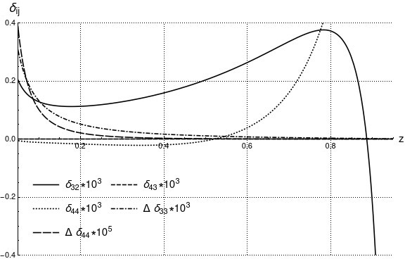
Figure 2: Higher-order contribution to the ISR radiator function.

IV Conclusions

In this way, we revisited the application of the QED structure function method for calculations of higher-order NLO ISR radiative corrections to $e^{+}e^{-}$ annihilation. A bug in the singlet part of the $\mathcal{O}(\alpha^{3}L^{3})$ of the electron PDF is corrected.

Several other issues that arose in earlier calculations of these corrections are clarified and improved. The relevance of positron in electron (and vice versa) PDF is demonstrated explicitly. Taking into account splitting of electron into positron (and vice versa) appears to be also significant in solutions of the QED evolution equations. Moreover, treatment of the factorization scale in NLO was refined. The issues listed above lead to a considerable difference of our results (both the leading and next-to-leading ones) from the ones given in [20].

The obtained results will be implemented into the ZFITTER computer code [34]. We would like to underline that the applied method leads to results being integrated over angular variables of the ISR radiation, and hence they can not take into account all possible experimental cuts. Nevertheless, first of all, one can use our results as benchmarks to verify the precision of Monte Carlo codes. Moreover, after implementation of the completely differential two-loop radiative corrections in a Monte Carlo code, one can add certain higher-order corrections in the collinear approximation without spoiling the theoretical precision too much. Extension of the presented here results to higher orders, like $c_{55}$ and $c_{54}$ is straightforward. The corresponding results will be presented elsewhere.

*

Appendix A Results as functions of $z$

Here, we show explicit results for the higher-order coefficients $c_{kl}$ from Eq. (6) as functions of the energy fraction $z$.

$$c^{\Theta}_{33}=-\frac{461}{18}-\frac{7z}{18}+\frac{710}{27(1-z)}+\frac{16}{27z}+\zeta_{2}\biggl{(}16z-\frac{32}{1-z}$$

$$+16\biggr{)}+\biggl{(}\frac{44z}{3}+\frac{44}{3}\biggr{)}\mathrm{Li}_{2}(1-z)+\frac{8z^{2}}{27(1-z)}-\frac{16z^{2}}{27}$$

$$+\biggl{(}\frac{40z^{2}}{9}+\frac{128z}{9}-\frac{88}{3(1-z)}+\frac{242}{9}\biggr{)}\ln(z)$$

$$+\biggl{[}-\frac{40z^{2}}{9}-\frac{50z}{3}+\frac{176}{3(1-z)}+\frac{40}{9z}+\biggl{(}\frac{92z}{3}-\frac{32}{1-z}+\frac{92}{3}\biggr{)}$$

$$\times\ln(z)-42\biggr{]}\ln(1-z)+\biggl{(}-16z+\frac{32}{1-z}-16\biggr{)}\ln^{2}(1-z)$$

$$+\biggl{(}-\frac{19z}{3}+\frac{16}{3(1-z)}-\frac{19}{3}\biggr{)}\ln^{2}(z)$$ (24)

$$c^{\Theta}_{44}(z)=-\frac{18779}{432}+\frac{4z^{2}}{27(1\!-\!z)}+\frac{328z^{2}}{81}+\frac{1115z}{432}+\frac{1108}{27(1-z)}$$

$$-\frac{328}{81z}+\zeta_{2}\biggl{(}\frac{68z^{2}}{9}+\frac{113z}{3}-\frac{128}{1-z}-\frac{68}{9z}+\frac{271}{3}\biggr{)}$$

$$+\zeta_{3}\biggl{(}-\frac{64z}{3}+\frac{128}{3(1-z)}-\frac{64}{3}\biggr{)}+\ln z\biggl{[}\frac{1145}{24}+\frac{64z^{2}}{27}$$

$$-\frac{241z}{72}-\frac{1708}{27(1-z)}-\frac{32}{27z}+\zeta_{2}\biggl{(}-\frac{32z}{3}+\frac{64}{3(1-z)}$$

$$-\frac{32}{3}\biggr{)}+\biggl{(}\frac{136z^{2}}{9}+\frac{194z}{3}-\frac{128}{1-z}+\frac{352}{3}\biggr{)}\ln(1-z)$$

$$+\biggl{(}\frac{178z}{3}-\frac{64}{1-z}+\frac{178}{3}\biggr{)}\ln^{2}(1-z)\biggr{]}+\ln(1-z)\biggl{[}-\frac{32z^{2}}{9}$$

$$-\frac{659z}{54}+\frac{32}{9z}+\frac{3416}{27(1-z)}-\frac{6173}{54}+\zeta_{2}\biggl{(}64z-\frac{128}{1-z}+64\biggr{)}\biggr{]}$$

$$+\biggl{[}27+\frac{68z^{2}}{9}+27z+\frac{68}{9z}+\biggl{(}\frac{164z}{3}+\frac{164}{3}\biggr{)}+\biggl{(}\!-38z$$

$$+\frac{64}{3(1-z)}-38\!\biggr{)}\ln z\biggr{]}\mathrm{Li}_{2}(1-z)+\biggl{(}-\frac{164z}{3}-\frac{164}{3}\biggr{)}$$

$$\times\mathrm{Li}_{3}(1\!-\!z)+\biggl{(}-\frac{146z}{3}+\frac{128}{3(1-z)}-\frac{146}{3}\biggr{)}\mathrm{Li}_{3}(z)$$

$$+\biggl{[}\!-\frac{68z^{2}}{9}-\frac{113z}{3}+\frac{128}{1\!-\!z}+\frac{68}{9z}-\frac{271}{3}\!\biggr{]}\ln^{2}(1-z)$$

$$+\biggl{[}-\frac{34z^{2}}{9}-\frac{275z}{24}+\frac{64}{3(1-z)}+\biggl{(}-\frac{146z}{3}+\frac{128}{3(1-z)}$$

$$-\frac{146}{3}\biggr{)}\ln(1-z)-\frac{187}{8}\biggr{]}\ln^{2}(z)+\biggl{(}6z+\frac{128}{3(1-z)}$$

$$+6\biggr{)}\ln^{3}(1-z)+\biggl{(}\frac{61z}{36}-\frac{16}{9(1-z)}+\frac{61}{36}\biggr{)}\ln^{3}(z),$$ (25)

$$\Delta c^{\Theta}_{44}(z)=\frac{1}{3}\biggl{[}\ln z\left(-21-\frac{16}{9z}-21z-\frac{16}{9}z^{2}\right)+\ln^{2}\!z\ (-2$$

$$+2z)+\ln^{3}\!z\!\left(\!-\frac{2}{3}-\frac{2}{3}z\!\right)\!-26-\frac{176}{27z}+26z+\frac{176}{27}z^{2}\!\biggr{]}.$$ (26)

$$c^{\Theta}_{32}(z)=\frac{1453}{9}-\frac{935z^{2}}{54(1-z)}-\frac{413z^{2}}{27}-\frac{910z}{9}-\frac{4967}{54(1-z)}$$

$$+\frac{584}{27z}+\biggl{(}\frac{10z^{2}}{9(1-z)}+\frac{32z^{2}}{9}-\frac{20z}{9}+\frac{146}{9(1-z)}-\frac{32}{9z}$$

$$-\frac{110}{9}\biggr{)}\zeta_{2}+\left(40+40z-\frac{40}{1-z}+\frac{24z^{2}}{1-z}\right)\zeta_{3}+\ln z\biggl{[}\frac{67}{9}$$

$$-\frac{1597z}{18}+\frac{214}{3(1-z)}\!-\frac{20}{9z}\!-\frac{100z^{2}}{9}+\left(8z\!-\frac{64}{3(1-z)}+\!8\right)\!\zeta_{2}$$

$$+\left(-28z+\frac{32}{1-z}-28\right)\mathrm{Li}_{2}(1-z)+\biggl{(}\frac{104z^{2}}{3}-\frac{154z}{3}$$

$$+\frac{224}{3(1-z)}-\frac{8}{3z}-\frac{328}{3}\biggr{)}\ln(1-z)+\left(10z+\frac{32}{1-z}+10\right)$$

$$\times\ln^{2}(1-z)\biggr{]}+\ln(1-z)\biggl{[}\frac{88z^{2}}{9(1-z)}+\frac{136z^{2}}{9}+\frac{1678z}{9}$$

$$-\frac{1768}{9(1-z)}-\frac{100}{9z}+\frac{142}{9}+\zeta_{2}\biggl{(}-\frac{16z}{3}+\frac{32}{3(1-z)}-\frac{16}{3}$$

$$+(52z+52)\mathrm{Li}_{2}(1-z)\biggr{)}\biggr{]}+\left(\frac{64z^{2}}{3}-40z+\frac{32}{3z}-46\right)$$

$$\times\mathrm{Li}_{2}(1-z)+(-52z-52)\mathrm{Li}_{3}(1-z)+\biggl{(}-40z$$

$$+\frac{64}{1-z}-40\biggr{)}\mathrm{Li}_{3}(z)+\biggl{(}-\frac{20z^{2}}{3}+\frac{16z}{3}-\frac{92}{3(1-z)}$$

$$+\left(-4z-\frac{16}{1-z}-4\right)\ln(1-z)+\frac{185}{6}\biggr{)}\ln^{2}(z)+\biggl{(}-\frac{52z^{2}}{3}$$

$$+19z-\frac{64}{1-z}+\frac{52}{3z}+45\biggr{)}\ln^{2}(1-z)+\biggl{(}-\frac{23z}{3}+\frac{32}{3(1-z)}$$

$$-\frac{23}{3}\biggr{)}\ln^{3}(z),$$ (27)

$$c^{\Theta}_{43}=\frac{183425}{648}-\frac{35281}{162(1-z)}+\frac{1366}{27z}-\frac{3259z^{2}}{162(1-z)}$$

$$-\frac{730z^{2}}{27}-\frac{76361z}{648}+\biggl{(}\frac{1292z^{2}}{27(1-z)}-\frac{512z^{2}}{27}-\frac{3245z}{9}$$

$$+\frac{12524}{27(1-z)}-\frac{19}{9}-\frac{208}{27z}\biggr{)}\zeta_{2}+\biggl{(}-\frac{56z^{2}}{3(1-z)}-\frac{80z^{2}}{9}$$

$$-\frac{632z}{9}-\frac{392}{3(1-z)}+\frac{244}{9}+\frac{1168}{9z}\biggr{)}\zeta_{3}+\biggl{(}-\frac{2092z}{3}$$

$$+\frac{320}{1-z}-\frac{2042}{3}\biggr{)}\zeta_{4}+\biggl{(}\frac{77z}{12}-\frac{16}{3(1-z)}+\frac{211}{36}\biggr{)}\ln^{4}(z)$$

$$+\biggl{[}\frac{152z^{2}}{27}-\frac{329z}{27}+\frac{376}{9(1-z)}-\frac{1693}{54}+\biggl{(}-176z$$

$$+\frac{512}{3(1-z)}-176\biggr{)}\ln(1-z)\biggr{]}\ln^{3}(z)+\biggl{[}\frac{364z^{2}}{27}$$

$$-\frac{2780}{27(1-z)}+\frac{1297}{9}+\frac{88}{27z}+\frac{947z}{9}+\biggl{(}\frac{152z}{3}-\frac{192}{1-z}$$

$$+\frac{152}{3}\biggr{)}\ln^{2}(1-z)+\zeta_{2}\biggl{(}14z+\frac{64}{1-z}+\frac{62}{3}\biggr{)}+\biggl{(}-80z^{2}$$

$$+\frac{620z}{9}-\frac{368}{3(1-z)}+\frac{1556}{9}-\frac{160}{9z}\biggr{)}\ln(1-z)+\biggl{(}-\frac{40z^{2}}{9}$$

$$+\frac{10z}{3}+\frac{10}{3}-\frac{40}{9z}\biggr{)}\ln(1+z)\biggr{]}\ln^{2}(z)+\biggl{[}-\frac{7795}{108}+\frac{344}{27z}$$

$$-\frac{1850z^{2}}{81}+\frac{13813z}{54}+\frac{6947}{27(1-z)}+\biggl{(}12z+\frac{64}{1-z}+12\biggr{)}$$

$$\times\ln^{3}(1-z)+\biggl{(}88z^{2}-\frac{994z}{9}+\frac{688}{3(1-z)}-\frac{2356}{9}+\frac{16}{3z}\biggr{)}$$

$$\times\ln^{2}(1-z)+\biggl{(}-\frac{1000z^{2}}{27}-\frac{17582z}{27}+\frac{12100}{27(1-z)}-\frac{6950}{27}$$

$$-\frac{296}{27z}+\zeta_{2}\biggl{(}\frac{1208z}{3}-\frac{448}{1-z}+\frac{1208}{3}\biggr{)}\biggr{)}\ln(1-z)$$

$$+\biggl{(}-\frac{224z^{2}}{9}+\frac{974z}{9}-\frac{1472}{3(1-z)}+\frac{3410}{9}+\frac{272}{9z}\biggr{)}\zeta_{2}$$

$$+\biggl{(}-\frac{40z^{2}}{3}+\frac{320z}{9}+\frac{320}{9}-\frac{40}{3z}\biggr{)}\ln(1+z)$$

$$+\biggl{(}60z+\frac{160}{1-z}+\frac{260}{3}\biggr{)}\zeta_{3}\biggr{]}\ln(z)+\biggl{[}-\frac{88z^{2}}{3}+\frac{62z}{3}$$

$$-\frac{256}{3(1-z)}+\frac{194}{3}+\frac{88}{3z}\biggr{]}\ln^{3}(1-z)+\biggl{(}\frac{80z^{2}}{27}-\frac{20z}{9}-\frac{20}{9}$$

$$+\frac{80}{27z}\biggr{)}\ln^{3}(1+z)+\biggl{[}\frac{584z^{2}}{27}+\frac{7675z}{18}-\frac{1376}{3(1-z)}+\frac{341}{18}$$

$$-\frac{224}{27z}+\zeta_{2}\biggl{(}-224z+\frac{448}{1-z}-224\biggr{)}\biggr{]}\ln^{2}(1-z)+\biggl{(}-168z$$

$$+\frac{64}{1-z}-168\biggr{)}\mathrm{Li}^{2}_{2}(1-z)+\biggl{(}\frac{40}{3}-\frac{40z}{3}\biggr{)}\mathrm{H}(-3,0,z)$$

$$+\biggl{(}-\frac{1348z}{3}+\frac{1088}{3(1-z)}-\frac{1348}{3}\biggr{)}\mathrm{H}(3,0,z)+\biggl{(}\frac{80z}{3}-\frac{80}{3}\biggr{)}$$

$$\times\mathrm{H}(-2,-1,0,z)+\biggl{(}\frac{40}{3}-\frac{40z}{3}\biggr{)}\mathrm{H}(-2,0,0,z)+\biggl{(}-320z$$

$$+\frac{640}{1-z}-320\biggr{)}\mathrm{H}(1,2,0,z)+\biggl{(}-336z+\frac{1088}{3(1-z)}-336\biggr{)}$$

$$\times\mathrm{H}(2,0,0,z)+\biggl{(}-592z+\frac{640}{1-z}-592\biggr{)}\mathrm{H}(2,1,0,z)$$

$$+\biggl{(}-96z+\frac{192}{1-z}-96\biggr{)}\mathrm{H}(1,0,0,0,z)+\biggl{(}-256z+\frac{512}{1-z}$$

$$-256\biggr{)}\mathrm{H}(1,1,0,0,z)+\biggl{(}-320z+\frac{640}{1-z}-320\biggr{)}$$

$$\times\mathrm{H}(1,1,1,0,z)+\biggl{(}-\frac{80z^{2}}{9}+\frac{20z}{3}+\frac{20}{3}-\frac{80}{9z}\biggr{)}\zeta_{2}\ln(1+z)$$

$$+\biggl{[}-\frac{208z^{2}}{9}-\frac{2089z}{9}+(132z+132)\ln^{2}(1-z)$$

$$+\biggl{(}-\frac{400z}{3}+\frac{256}{3(1-z)}-\frac{400}{3}\biggr{)}\ln^{2}z+\biggl{(}\frac{752z^{2}}{9}-\frac{1412z}{9}$$

$$-\frac{1160}{9}+\frac{928}{9z}\biggr{)}\!\ln(\!1-z\!)+\zeta_{2}\biggl{(}\frac{536z}{3}+\frac{536}{3}\biggr{)}+\biggl{(}-\frac{608z^{2}}{9}$$

$$+\frac{344z}{9}+\biggl{(}-\frac{464z}{3}+\frac{128}{1-z}-\frac{464}{3}\biggr{)}\ln(1-z)+\frac{256}{3(1-z)}$$

$$-\frac{40}{9}-\frac{272}{9z}\biggr{)}\ln(z)-\frac{725}{3}-\frac{104}{9z}\biggr{]}\mathrm{Li}_{2}(1-z)+\biggl{[}-\frac{40z^{2}}{3}$$

$$+\frac{320z}{9}+\zeta_{2}\biggl{(}\frac{40}{3}-\frac{40z}{3}\biggr{)}+\biggl{(}\frac{80z^{2}}{9}+\frac{40z}{3}-\frac{40}{3}-\frac{80}{9z}\biggr{)}\ln(z)$$

$$+\frac{320}{9}-\frac{40}{3z}\biggr{]}\mathrm{Li}_{2}(-z)+\biggl{[}-\frac{752z^{2}}{9}+\frac{1412z}{9}-(264z+264)$$

$$\times\ln(1-z)+\biggl{(}-\frac{544z}{3}-\frac{544}{3}\biggr{)}\ln(z)+\frac{1160}{9}-\frac{928}{9z}\biggr{]}$$

$$\times\mathrm{Li}_{3}(1-z)+\biggl{(}-\frac{80z^{2}}{3}-20z+\frac{100}{3}+\frac{80}{9z}\biggr{)}\mathrm{Li}_{3}(-z)$$

$$+\biggl{[}-\frac{608z^{2}}{9}+\frac{74z}{9}+\biggl{(}256z-\frac{512}{1-z}+256\biggr{)}\ln(1-z)$$

$$+\biggl{(}-176z+\frac{512}{3(1-z)}-176\biggr{)}\ln(z)+\frac{512}{3(1-z)}-\frac{334}{9}$$

$$-\frac{320}{9z}\biggr{]}\mathrm{Li}_{3}(z)+\biggl{(}-\frac{160z^{2}}{9}+\frac{40z}{3}+\frac{40}{3}-\frac{160}{9z}\biggr{)}\mathrm{Li}_{3}\biggl{(}\frac{1}{1+z}\biggr{)}$$

$$+\biggl{(}584z-\frac{640}{1-z}+584\biggr{)}\mathrm{Li}_{4}(1-z)+\biggl{(}-284z+\frac{192}{1-z}$$

$$-284\biggr{)}\mathrm{Li}_{4}(z)+\biggl{(}532z-\frac{768}{1-z}+532\biggr{)}\mathrm{S}_{2,2}(z)+\biggl{[}\frac{572z^{2}}{27(1-z)}$$

$$+\frac{1226z^{2}}{81}-\frac{5680}{9(1-z)}-\frac{3205z}{27}+\frac{2345}{3}-\frac{2090}{81z}+\biggl{(}\frac{752z^{2}}{9}$$

$$-\frac{64z^{2}}{3(1-z)}+-\frac{340z}{3}+\frac{1376}{3(1-z)}-\frac{1100}{3}-\frac{752}{9z}\biggr{)}\zeta_{2}$$

$$+\biggl{(}-288z+\frac{576}{1-z}-288\biggr{)}\zeta_{3}\biggr{]}\ln(1-z).$$ (28)

$$c_{33}^{\Delta}=\biggl{(}\frac{718}{27}-32\zeta_{2}\biggr{)}\ln\Delta+\frac{88}{3}\ln^{2}\Delta+\frac{32}{3}\ln^{3}\Delta+\frac{143}{18}$$

$$+\frac{64}{3}\zeta_{3}-\frac{88}{3}\zeta_{2},$$ (29)

$$c_{44}^{\Delta}=\biggl{(}\frac{1112}{27}+\frac{256}{3}\zeta_{3}-128\zeta_{2}\biggr{)}\ln\Delta+\biggl{(}\frac{1708}{27}-64\zeta_{2}\biggr{)}$$

$$\times\ln^{2}\Delta+\frac{128}{3}\ln^{3}\Delta+\frac{32}{3}\ln^{4}\Delta+\frac{715}{72}+16\zeta_{4}+\frac{256}{3}\zeta_{3}$$

$$-\frac{1708}{27}\zeta_{2},$$ (30)

$$c_{32}^{\Delta}=\biggl{(}-\frac{2951}{27}+48\zeta_{3}+104\zeta_{2}\biggr{)}\ln\Delta+\biggl{(}32\zeta_{2}-\frac{280}{3}\biggr{)}\ln^{2}\Delta$$

$$-\frac{64}{3}\ln^{3}\Delta-\frac{1387}{36}-80\zeta_{4}+\frac{4}{3}\zeta_{3}+\frac{928}{9}\zeta_{2},$$ (31)

$$c_{43}^{\Delta}=-\frac{13969}{216}+\frac{1504\zeta_{2}\zeta_{3}}{3}+\frac{1465\zeta_{2}}{27}+\frac{314\zeta_{3}}{9}-\frac{488\zeta_{4}}{3}$$

$$-1024\zeta_{5}-\frac{64}{3}\ln^{4}\Delta+\left(\frac{896\zeta_{2}}{3}-\frac{1376}{9}\right)\ln^{3}\Delta+\biggl{(}\frac{1616\zeta_{2}}{3}$$

$$-672\zeta_{3}-\frac{8234}{27}\biggr{)}\ln^{2}\Delta+\biggl{(}\frac{16408\zeta_{2}}{27}-\frac{1856\zeta_{3}}{3}+320\zeta_{4}$$

$$-\frac{19270}{81}\biggr{)}\ln\Delta.$$ (32)

Here $H(a_{1},...,a_{k};z)$ are harmonic polylogarithms [35, 36].

References

• Abada et al. [2019] A. Abada et al. (FCC), FCC Physics Opportunities: Future Circular Collider Conceptual Design Report Volume 1, Eur. Phys. J. C 79, 474 (2019).
• Dong et al. [2018] M. Dong et al. (CEPC Study Group), CEPC Conceptual Design Report: Volume 2 - Physics & Detector,   (2018), arXiv:1811.10545 [hep-ex] .
• ILC [2013] The International Linear Collider Technical Design Report - Volume 2: Physics,   (2013), arXiv:1306.6352 [hep-ph] .
• Jadach and Skrzypek [2019] S. Jadach and M. Skrzypek, QED challenges at FCC-ee precision measurements, Eur. Phys. J. C 79, 756 (2019), arXiv:1903.09895 [hep-ph] .
• Note [1] The functions can be better called as QED parton distribution ones (QED PDFs).
• Kuraev and Fadin [1985] E. A. Kuraev and V. S. Fadin, On Radiative Corrections to e+ e- Single Photon Annihilation at High-Energy, Sov. J. Nucl. Phys. 41, 466 (1985).
• Engel et al. [2020] T. Engel, A. Signer, and Y. Ulrich, A subtraction scheme for massive QED, JHEP 01, 085, arXiv:1909.10244 [hep-ph] .
• Frixione [2021] S. Frixione, On factorisation schemes for the electron parton distribution functions in QED, JHEP 07, 180, [Erratum: JHEP 12, 196 (2012)], arXiv:2105.06688 [hep-ph] .
• Nicrosini and Trentadue [1987] O. Nicrosini and L. Trentadue, Soft Photons and Second Order Radiative Corrections to e+ e- —$>$ Z0, Phys. Lett. B 196, 551 (1987).
• Przybycien [1993] M. Przybycien, A Fifth order perturbative solution to the Gribov-Lipatov equation, Acta Phys. Polon. B 24, 1105 (1993), arXiv:hep-th/9511029 .
• Skrzypek [1992] M. Skrzypek, Leading logarithmic calculations of QED corrections at LEP, Acta Phys. Polon. B 23, 135 (1992).
• Cacciari et al. [1992] M. Cacciari, A. Deandrea, G. Montagna, and O. Nicrosini, QED structure functions: A Systematic approach, EPL 17, 123 (1992).
• Jadach et al. [2001] S. Jadach, B. F. L. Ward, and Z. Was, Coherent exclusive exponentiation for precision Monte Carlo calculations, Phys. Rev. D 63, 113009 (2001), arXiv:hep-ph/0006359 .
• Arbuzov et al. [2006a] A. B. Arbuzov, G. V. Fedotovich, F. V. Ignatov, E. A. Kuraev, and A. L. Sibidanov, Monte-Carlo generator for e+e- annihilation into lepton and hadron pairs with precise radiative corrections, Eur. Phys. J. C 46, 689 (2006a), arXiv:hep-ph/0504233 .
• Actis et al. [2010] S. Actis et al. (Working Group on Radiative Corrections, Monte Carlo Generators for Low Energies), Quest for precision in hadronic cross sections at low energy: Monte Carlo tools vs. experimental data, Eur. Phys. J. C 66, 585 (2010), arXiv:0912.0749 [hep-ph] .
• Berends et al. [1988] F. A. Berends, W. L. van Neerven, and G. J. H. Burgers, Higher Order Radiative Corrections at LEP Energies, Nucl. Phys. B 297, 429 (1988), [Erratum: Nucl.Phys.B 304, 921 (1988)].
• Arbuzov and Melnikov [2002] A. Arbuzov and K. Melnikov, O(alpha**2 ln(m(mu) / m(e)) corrections to electron energy spectrum in muon decay, Phys. Rev. D 66, 093003 (2002), arXiv:hep-ph/0205172 .
• Blumlein and Kawamura [2003] J. Blumlein and H. Kawamura, O(alpha**2 L) radiative corrections to deep inelastic ep scattering, Phys. Lett. B 553, 242 (2003), arXiv:hep-ph/0211191 .
• Arbuzov and Scherbakova [2006] A. B. Arbuzov and E. S. Scherbakova, Next-to-leading order corrections to Bhabha scattering in renormalization group approach. I. Soft and virtual photonic contributions, JETP Lett. 83, 427 (2006), arXiv:hep-ph/0602119 .
• Ablinger et al. [2020] J. Ablinger, J. BlĂŒmlein, A. De Freitas, and K. Schönwald, Subleading Logarithmic QED Initial State Corrections to e+​e−→γ∗/Z0∗→superscript𝑒superscript𝑒superscriptđ›Ÿsuperscriptsuperscript𝑍0e^{+}e^{-}\rightarrow\gamma^{*}/{Z^{0}}^{*} to O​(α6​L5)𝑂superscriptđ›Œ6superscript𝐿5O(\alpha^{6}L^{5}), Nucl. Phys. B 955, 115045 (2020), arXiv:2004.04287 [hep-ph] .
• Bertone et al. [2020] V. Bertone, M. Cacciari, S. Frixione, and G. Stagnitto, The partonic structure of the electron at the next-to-leading logarithmic accuracy in QED, JHEP 03, 135, [Erratum: JHEP 08, 108 (2022)], arXiv:1911.12040 [hep-ph] .
• Arbuzov and Voznaya [2023] A. B. Arbuzov and U. E. Voznaya, Unpolarized QED parton distribution functions in NLO, J. Phys. G 50, 125004 (2023), arXiv:2212.01124 [hep-ph] .
• Arbuzov and Voznaya [2024] A. B. Arbuzov and U. E. Voznaya, Higher-order NLO radiative corrections to polarized muon decay spectrum, Phys. Rev. D 109, 053001 (2024), arXiv:2312.10778 [hep-ph] .
• Arbuzov [2019] A. B. Arbuzov, Leading and Next-to-Leading Logarithmic Approximations in Quantum Electrodynamics, Phys. Part. Nucl. 50, 721 (2019).
• Ellis and Vogelsang [1996] R. K. Ellis and W. Vogelsang, The Evolution of parton distributions beyond leading order: The Singlet case,   (1996), arXiv:hep-ph/9602356 .
• Furmanski and Petronzio [1980] W. Furmanski and R. Petronzio, Singlet Parton Densities Beyond Leading Order, Phys. Lett. B 97, 437 (1980).
• Mele and Nason [1991] B. Mele and P. Nason, The Fragmentation function for heavy quarks in QCD, Nucl. Phys. B 361, 626 (1991), [Erratum: Nucl.Phys.B 921, 841–842 (2017)].
• Frixione [2019] S. Frixione, Initial conditions for electron and photon structure and fragmentation functions, JHEP 11, 158, arXiv:1909.03886 [hep-ph] .
• Blumlein et al. [2012] J. Blumlein, A. De Freitas, and W. van Neerven, Two-loop QED Operator Matrix Elements with Massive External Fermion Lines, Nucl. Phys. B 855, 508 (2012), arXiv:1107.4638 [hep-ph] .
• Andonov et al. [2010] A. Andonov, A. Arbuzov, S. Bondarenko, P. Christova, V. Kolesnikov, G. Nanava, and R. Sadykov, NLO QCD corrections to Drell-Yan processes in the SANC framework, Phys. Atom. Nucl. 73, 1761 (2010), arXiv:0901.2785 [hep-ph] .
• Note [2] Such a choice is not justified by the known result for one-loop ISR corrections.
• Gorishnii et al. [1991] S. G. Gorishnii, A. L. Kataev, and S. A. Larin, The three loop QED contributions to the photon vacuum polarization function in the MS scheme and the four loop corrections to the QED beta function in the on-shell scheme, Phys. Lett. B 273, 141 (1991), [Erratum: Phys.Lett.B 275, 512 (1992), Erratum: Phys.Lett.B 341, 448 (1995)].
• Baikov et al. [2013] P. A. Baikov, K. G. Chetyrkin, J. H. Kuhn, and C. Sturm, The relation between the QED charge renormalized in MSbar and on-shell schemes at four loops, the QED on-shell beta-function at five loops and asymptotic contributions to the muon anomaly at five and six loops, Nucl. Phys. B 867, 182 (2013), arXiv:1207.2199 [hep-ph] .
• Arbuzov et al. [2006b] A. B. Arbuzov, M. Awramik, M. Czakon, A. Freitas, M. W. Grunewald, K. Monig, S. Riemann, and T. Riemann, ZFITTER: A Semi-analytical program for fermion pair production in e+ e- annihilation, from version 6.21 to version 6.42, Comput. Phys. Commun. 174, 728 (2006b), arXiv:hep-ph/0507146 .
• Maitre [2006] D. Maitre, HPL, a mathematica implementation of the harmonic polylogarithms, Comput. Phys. Commun. 174, 222 (2006), arXiv:hep-ph/0507152 .
• Ablinger et al. [2019] J. Ablinger, J. BlĂŒmlein, M. Round, and C. Schneider, Numerical Implementation of Harmonic Polylogarithms to Weight w = 8, Comput. Phys. Commun. 240, 189 (2019), arXiv:1809.07084 [hep-ph] .