Prediction of the amplitude of solar cycle 25 from the ratio of sunspot number to sunspot-group area, low latitude activity, and 130-year solar cycle

Abstract

Prediction of the amplitude of solar cycle is important for understanding the mechanism of solar cycle and solar activity influence on space-weather. We analysed the combined data of sunspot groups from Greenwich Photoheliographic Results (GPR) during the period 1874 – 1976 and Debrecen Photoheliographic Data (DPD) during 1977 – 2017 and determined the monthly mean, annual mean, and 13-month smoothed monthly mean whole sphere sunspot-group area (WSGA). We also analysed the monthly mean, annual mean, and 13-month smoothed monthly mean version 2 of international sunspot number ($SN_{\rm T}$) during the period 1874 – 2017. We fitted the annual mean WSGA and $SN_{\rm T}$ data during each of Solar Cycles 12 – 24 separately to the linear and nonlinear (parabola) forms. In the cases of Solar Cycles 14, 17, and 24 the nonlinear fits are found better than the linear fits. We find that there exists a secular decreasing trend in the slope of the WSGA–$SN_{\rm T}$ linear relation during Solar Cycles 12 – 24. A secular decreasing trend is also seen in the coefficient of the first order term of the nonlinear relation. The existence of $\approx$77-year variation is clearly seen in the ratio of the amplitude to WSGA at the maximum epoch of solar cycle. From the pattern of this long-term variation of the ratio we inferred that Solar Cycle 25 will be larger than both Solar Cycles 24 and 26. Using an our earlier method (now slightly revised), i.e. using high correlations of the amplitude of a solar cycle with the sums of the areas of sunspot groups in $0$ – $10^{\circ}$ latitude intervals of the northern hemisphere during 3.75-year interval around the minimum–and the southern hemisphere during 0.4-year interval near the maximum–of the corresponding preceding solar cycle, we predicted $127\pm 26$ and $141\pm 19$ for the amplitude of Solar Cycle 25, respectively. Based on $\approx$130-year periodicity found in the cycle-to-cycle variation of the amplitudes of Solar Cycles 12 – 24 we find the shape of Solar Cycle 25 would be similar to that of Solar Cycle 13 and predicted for Solar Cycle 25 the amplitude $135\pm 8$, maximum epoch 2024.21 (March 2024)$\pm$6-month, and the following minimum epoch 2032.21 (March 2032)$\pm$6-month with $SN_{\rm T}$ $\approx 4$.

1 Introduction

Prediction of the amplitude of solar cycle is very important because it helps for understanding the mechanism of solar cycle, solar activity influence on space weather, and solar-Terrestrial relationship (Hathaway, 2015). Many techniques are used for predicting the amplitudes of Solar Cycles 24 and 25 (Pesnell, 2012; Petrovay, 2020; Nandy, 2021). The sunspot number and sunspot area are the most prominently used indece of solar activity to study characteristics of solar cycles and to investigate other short- and long-term variations of solar activity. It is well-known that there exists a good linear relationship between the maximum sunspot number and the maximum sunspot area of solar cycles (e.g., Hathaway et al., 2002; Javaraiah, 2022). However, the characteristics of sunspot-number cycles and sunspot-area cycles are not exactly the same. In some solar cycles the epochs of maxima of sunspot number and sunspot area are to some extent different (Ramesh and Rohini, 2008). The ratio of monthly or yearly mean sunspot area to sunspot number varies during a solar cycle, it is large during maximum and least during minimum of a solar cycle. However, in many solar cycles there exist considerable differences in the positions of the maximum and minimum of the ratio with respect to the corresponding sunspot number maximum and minimum (Wilson and Hathaway, 2006). The well-known Waldmeier effect of sunspot cycles (large cycles rise faster than the small cycles) seems not apply for sunspot-area cycles (Dikpati, et al., 2008; Javaraiah, 2019). However, Karak and Choudhuri (2011) by correcting the positions of the area-peaks of some solar cycles obtained an anticorrelation between rise time and amplitude. There exits a good correlation between rise rate and amplitude (Karak and Choudhuri, 2011; Kumar et al., 2022). Large and small sunspots/sunspot-groups are not in the same propositions in all solar cycles and there exist differences in their variations during solar cycles (Kilcik et al., 2011; Javaraiah, 2012, 2021; Clette and Lefévre, 2016; Mandal et al., 2016). Moreover, sunspot areas are thought to be more physical measures of solar activity (Hathaway, 2015). It is believed that sunspot area represents the solar magnetic flux better than sunspot number.

In this analysis we determined the correlation between the annual mean values of total (north $+$ south) sunspot number $SN_{\rm T}$ and the annual mean area (WSGA) of the sunspot groups in whole sphere (north $+$ south) during each of Solar Cycles 12 – 24, separately. We fitted the annual mean values of WSGA and $SN_{\rm T}$ during each of Solar Cycles 12 – 24 separately to the linear and nonlinear (parabola) forms. In a few solar cycles the fit of the nonlinear form is found better than the linear form. We show that there exists a secular decreasing trend in the slope of the WSGA–$SN_{\rm T}$ linear relation during Solar Cycles 12 – 24. We also show that there exists a secular decreasing trend mainly in the coefficient of the first order term of the nonlinear relation. In this analysis we also determined the solar cycle-to-cycle variation in the ratio of the smoothed monthly mean maximum value of $SN_{\rm T}$ (i.e. the amplitude $R_{\rm M}$) of a solar cycle to the smoothed monthly mean value of WSGA at the maximum epoch of the solar cycle. Based on the pattern of this variation we make predictions for the relative amplitudes of some upcoming solar cycles. By making a minor change in our earlier method that based on low latitude activity (Javaraiah, 2007, 2008) we have made improved predictions for the amplitude of Solar Cycle 25. Recently, (Javaraiah, 2022, 2023), we have noticed that there exists a $\approx$130-year periodicity in the amplitude ($R_{\rm M}$) modulation during Solar Cycles 12 – 24. The uncertainty in this periodicity is to some extent large because it is determined from only 13 sunspot cycles’ data. However, this periodicity is found in the huge data of solar activity related phenomena, such as ${}^{14}C$ and ${}^{10}Be$ (Attolini et al., 1990a, b; McCracken et al., 2013). On the basis of this periodicity we find that the shape of Solar Cycle 24 is similar to that of Solar Cycle 12 and the rising phase of Solar Cycle 25 is similar to that of Solar Cycle 13. Using it we predict the shape of Solar Cycle 25 will be similar to that of Solar Cycle 13 and predict the amplitude, maximum epoch, and the ending epoch of Solar Cycle 25.

In the next section we describe the data and analysis. In Section 3 we present the results. In Section 4 we present the conclusions and discuss them.

2 Data and analysis

We have used the data of sunspot groups from Greenwich Photoheliographic Results (GPR) during the period 1874 – 1976 and Debrecen Photoheliographic Data (DPD) during the period 1977 – 2017. These data are downloaded from the website fenyi.solarobs.unideb.hu/pub/DPD/. These data contain heliographic positions (latitude and longitude), the corrected whole-spot area ($A$), central meridian distance (CMD), etc. for each sunspot group for each day during its lifetime (disk passage). In order to reduce the foreshortening effect (if any) we have used only the values of $A$ correspond to the $|{\rm CMD}|\leq 75^{\circ}$. We determined the mean whole sphere sunspot-group area (WSGA) of each month during the period 1874 – 2017 and then we obtained the time series of 13-month smoothed monthly mean and annual mean values of WSGA. We have used the time series of 13-month smoothed monthly mean values, monthly mean values, and annual values of version-2 of the total international sunspot number ($SN_{\rm T}$) during the period 1874 – 2023 (downloaded the files SN_ms_tot_v2.0.txt, SN_m_tot_v2.0.txt, and SN_y_tot_v2.0.txt from the website www.sidc.be/silso/datafiles). The subscript ‘T’ of $SN_{\rm T}$ indicates northern and southern hemispheres’ total. All these time series are partitioned for individual Solar Cycles 12 – 24. We fitted each solar cycle’s annual mean values (also monthly and smoothed monthly values) of WSGA and $SN_{\rm T}$ to the linear from:

$$SN_{\rm T}=m\times{\rm WSGA},$$ (1)

and also to the nonlinear from:

$$SN_{\rm T}=m_{1}\times{\rm WSGA}+m_{2}\times{\rm WSGA}^{2}.$$ (2)

Both these equations are forced to pass through the origin by assuming $SN_{\rm T}$ is zero when WSGA is zero. The linear least-square fits are calculated by using the Interactive Digital Library (IDL) software FITEXY.PRO, which is downloaded from the website http: //idlastro.gsfc.nasa.gov/ftp/pro/math/. An advantage of this software is it takes care the uncertainties in the values of both the abscissa (WSGA) and ordinate ($SN_{\rm T}$) in the calculations of linear-least-square fit. The nonlinear fit is done by taking into account only the uncertainties in $SN_{\rm T}$ (in the available software there is no provision for using the errors in the abscissa). We also determined the solar cycle-to-cycle variation of the ratio $R_{\rm M}/R_{A}$ during Solar Cycles 12 – 24, where the amplitude $R_{\rm M}$ and $R_{A}$ are the 13-month smoothed monthly mean values of $SN_{\rm T}$ and WSGA, respectively, at the maximum epoch of a solar cycle (this is also done by using the corresponding annual mean values).

In our earlier papers, (Javaraiah, 2015, 2017, 2021, 2023), based on an high correlation was found between the amplitude ($R_{\rm M}$) of a solar cycle and the sum of the areas ($A^{*}_{\rm M}$) of the sunspot groups in $0$ – $10^{\circ}$ latitude interval of the southern hemisphere during a slightly less than one-year time interval ($T^{*}_{\rm M}$) just after the maximum of the solar cycle (namely REL-I), we have predicted that the amplitude of Solar Cycle 25 will be considerably weaker than the amplitude of the reasonably small Solar Cycle 24. That prediction is incorrect (the height of the rising phase of Solar Cycle 25 is already higher than that of Solar Cycle 24). On the other hand, all our earlier analyses suggest a low amplitude for Solar Cycle 25. As per the current trend of activity this suggestion is expected to be holds good, although this cycle will be slightly larger than Solar Cycle 24. In addition, based on the pattern of the cycle-to-cycle variation in the aforementioned sum of the areas of the sunspot groups we also predicted as Solar Cycle 25 will be larger than Solar Cycle 24 (Javaraiah, 2008), which is consistent with the current trend of the rising phase of Solar Cycle 25.

Earlier, (Javaraiah, 2007), we have also found an high correlation between the amplitude of a solar cycle and the sum of the areas ($A^{*}_{\rm m}$) of sunspot groups in $0$ – $10^{\circ}$ latitude interval of the northern hemisphere during about 3.5-year time interval ($T^{*}_{\rm m}$) around the preceding minimum of previous solar cycle (namely REL-II). However, the corresponding correlation of this relationship (REL-II) is relatively smaller than that was obtained by using REL-I and also the uncertainty in the predicted value of the amplitude of Solar Cycle 24 was found relatively large. Later the predicted amplitude of Solar Cycle 24 was found considerably larger than the observed value. The corresponding prediction made by using REL-I was found closely match with the observed value. Therefore, in Javaraiah (2015, 2017) we have not used REL-II for predicting the amplitude of Solar Cycle 25. In Javaraiah (2021) we have used REL-II and obtained $123\pm 23$ for the amplitude of Solar Cycle 25, but this prediction was not claimed there.

Here we analysed the GPR and DPD sunspot group data during 1874 – 2017 and as in Javaraiah (2007, 2008) we determine the relations REL-I and REL-II by taking into account the uncertainties in the values of the maxima of Solar Cycles 12 – 24 and making corrections to the values of $T^{*}_{\rm M}$ of Solar Cycles 23 and 24. Using the improved relations REL-I and REL-II we make improvements in our earlier predictions of the amplitude of Solar Cycle 25.

Based on the existence of a $\approx$12-cycle ($\approx$130-year) periodicity in the variation of a $R_{\rm M}$ during Solar Cycles 12 – 24 (Javaraiah, 2022, 2023) we found that the shape of Solar Cycle 24 is similar to that of Solar Cycle 12 and the rising phase of Solar Cycle 25 (for which the values of $SN_{\rm T}$ are available) is similar to that of Solar Cycle 13. We find a high correlation between the variation in the 13-month smoothed monthly mean $SN_{\rm T}$ during Solar Cycles 12 – 13 (rise phase) and that during Solar Cycles 24 – 25 (rise phase). The corresponding linear-least-square best-fit is used to simulate the Solar Cycles 25 – 26.

3 Results

3.1 Relationship between sunspot number and sunspot-group area

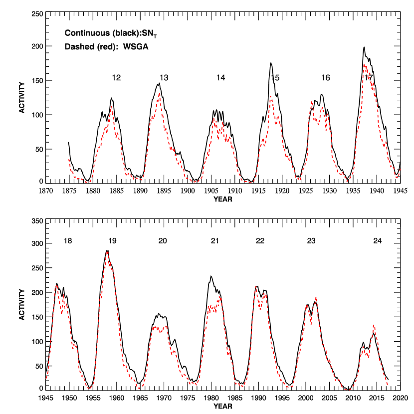
Figure 1: Variations in the 13-month smoothed monthly mean version 2 of international sunspot number $SN_{\rm T}$ (black continuous-curve) and the corresponding smoothed area of the sunspot groups in the whole sphere WSGA (red dashed-curve) during the period 1874 – 2017. The values of WSGA is first divided by the largest value of WSGA, 3480.15 msh, and then multiplied by the largest value, 285.0 of $SN_{\rm T}$. Waldmeier numbers of the solar cycles are also shown.

Fig. 1 shows variations in the 13-month smoothed monthly mean version 2 of international sunspot number ($SN_{\rm T}$) and the corresponding smoothed area (WSGA) of the sunspot groups in the whole sphere during the period 1874 – 2017. As can be seen in this figure there are some noticeable differences in the variations of $SN_{\rm T}$ and WSGA, during many solar cycles (also see Javaraiah, 2019, 2020). A good agreement between the variations of $SN_{\rm T}$ and WSGA during the minima of most of the solar cycles, whereas some considerable differences exist during the maxima of many solar cycles. That is, although the positions of the peaks during the maxima (i.e., Gnevyshev peaks) of $SN_{\rm T}$-cycles and WSGA-cycles are almost the same, but in some cycles (e.g., 16 and 21) the main (highest) and second high (secondary) peaks are interchanged. In the case of some solar cycles (16, 17, 20, 21) the heights of the peaks of WSGA are relatively lower than those of $SN_{\rm T}$, and it seems opposite in Solar Cycles 23 and 24 (see the main peaks).

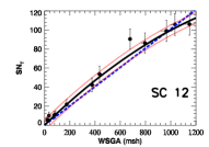
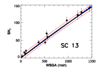
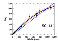
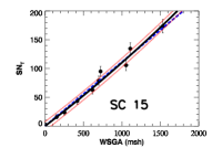
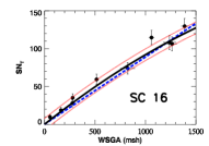
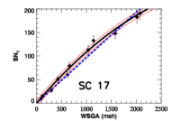
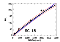
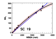
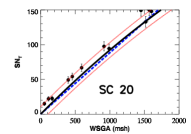
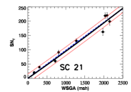
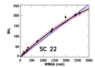
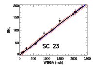
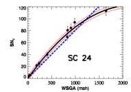
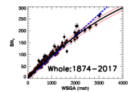
Figure 2: Scatter plots of the annual mean WSGA versus the annual mean $SN_{\rm T}$ of Solar Cycles 12 – 24. The horizontal and vertical error bars represent the errors in WSGA and $SN_{\rm T}$, respectively. The blue dashed-line represents best-fit linear relationship between WSGA and $R_{\rm M}$. The black continuous-curve represent the best fit non-linear relation and the red dotted-curve represents the corresponding one-rms (root-mean-square deviation) level.

Fig. 2 shows the relationship between $SN_{\rm T}$ and WSGA during each of Solar Cycles 12 – 24 and also during the whole period 1874 – 2017 determined by using the annual mean values of $SN_{\rm T}$ and WSGA (in the case of Solar Cycle 24 the data are incomplete). In this figure we have shown the best fit linear and nonlinear relations and the details such as values of slope/coefficients, correlation coefficient, $\chi^{2}$ and the corresponding probability ($P$), etc., are given in Tables 1 and 2. Table 1 also contains the values of $R_{\rm M}$ and the mean WSGA (13-month smoothed monthly mean values) at the maximum epoch and the corresponding uncertainties $\sigma_{\rm R}$ and $\sigma_{\rm A}$, respectively, of solar cycles. The linear least-square fit is calculated by taking into account the errors in the values of $SN_{\rm T}$, whereas the nonlinear fit is done by taking into account the errors in the values of $SN_{\rm T}$ only. Note that a small value of $P$ indicates a poor fit (large value of $\chi^{2}$). In the cases of all solar cycles and the whole period the correlation is good (significant on more than 99 % confidence level). As can be seen in Fig. 2 and Table 1, in all solar cycles and whole-period the obtained linear relations of WSGA and $SN_{\rm T}$ are good, in the sense that the ratio of slope to its uncertainty is substantially large. However, in the cases of several solar cycles (14, 17, 18, 19, 21, and 24) and whole period the value of $\chi^{2}$ is large ($P$ is small), i.e. $\chi^{2}$ is significant on more than 95 % confidence level. As can be seen in Fig. 2 and Table 2 in the nonlinear case the ratio of the coefficient ($m_{1}$) of the first order term to the corresponding uncertainty is reasonably large in all solar cycles and the corresponding ratio of the second order term is significant only in a few cycles (14, 17, and 24). In these cycles the $\chi^{2}$ is also insignificant. That is, for each of these cases the nonlinear fit is better than that of the linear fit. In the case of the whole period the $\chi^{2}$ value of the linear fit is slightly smaller than that of the nonlinear fit, i.e. in this case the linear fit seems to be slightly better than nonlinear fit. (Similar results are also found from the monthly mean and the 13-month smoothed monthly mean values of WSGA and $SN_{\rm T}$).

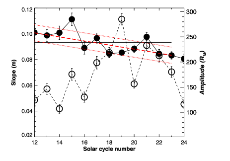
Figure 3: The filled circle-continuous curve represents solar cycle-to-cycle variation in the slope ($m$) of the linear relationship (Eq. (1)) of WSGA and $SN_{\rm T}$ during Solar Cycles 12 – 24, determined by using the corresponding annual mean values. The horizontal continuous-line represents the mean value of the slopes during Solar Cycles 12 – 23. The long-dashed line (red) represents the secular decreasing trend in the slope obtained from the best-fit linear relation (Eq. (3)) between the slope and solar cycle number during Solar Cycles 12 – 23, and the corresponding one-rms level is shown by the red dotted-line. The open circle-dashed curve represents the variation in the amplitude ($R_{\rm M}$) of solar cycle. The data point of the incomplete Solar Cycle 24 is not used for the determination of both the mean and the linear-least-square fit.

Fig. 3 shows the cycle-to-cycle variation in the slope ($m$) of the nonlinear relation between WSGA and $SN_{\rm T}$ during Solar Cycles 12 – 24. In this figure we have also shown the variation in the amplitude ($R_{\rm M}$) of solar cycle. The values of $R_{\rm M}$ of Solar Cycles 12 – 24 are taken from Pesnell (2018). As we can see in this figure there exists a considerable variation in the slope. The slope of the average Solar Cycle 15 is largest and is at about $2\sigma$ (standard deviation) level (significant on about 95% confidence level). No significant correlation is found between the slope and the amplitude ($R_{\rm M}$) of a solar cycle. There is a suggestion of the existence of a secular decreasing trend in the slope from Solar Cycle 12 – 24 and it seems superimposed on it a weak 77-year long-term variation (may be related to the Gleissberg cycle). We obtained the following linear relationship between the slope ($m$) and solar cycle number ($n$).

$$m=0.12\pm 0.0065-(0.00158\pm 0.00034)n$$ (3)

The corresponding correlation of this relation (Eq. (3)) is not very good ($r=-0.69$), but the least-square fit is reasonably good, i.e. the slope is reasonably well defined (the ratio of the slope to its standard deviation is about 5) and the rms (root-mean-square deviation) value 0.0063 is reasonably small (the data point of the incomplete Solar Cycle 24 is excluded for the determination of both the mean and the linear-least-square fit.)

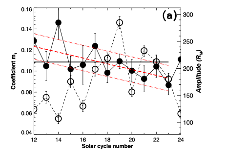
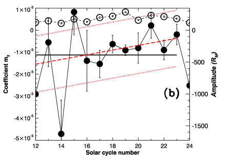
Figure 4: The filled circle-continuous curve represents solar cycle-to-cycle variation in (a) the coefficient $m_{1}$ and (b) the coefficient $m_{2}$ of the nonlinear relationship (Eq. (2)) of WSGA and $SN_{\rm T}$ during the whole Solar Cycles 12 – 24, determined by using the corresponding annual mean values. The horizontal continuous line represents the mean value of the coefficients during Solar Cycles 12 – 23. The long-dashed line (red) represents the secular trend in the coefficient obtained from the best-fit linear relation (Eq. (4)) between $m_{1}$ and the solar cycle number ($n$), and between $m_{2}$ and $n$ (Eq. (5), during Solar Cycles 12 – 23, and the corresponding one-rms level is shown by the red dotted-line. The open circle-dashed curve represents the variation in the amplitude ($R_{\rm M}$) of solar cycle. The data point of the incomplete Solar Cycle 24 is not used for the determination of both the mean and the linear least-square fit.

Figs. 4a and 4b show the cycle-to-cycle variations in the coefficients $m_{1}$ and $m_{2}$ of the nonlinear relation between WSGA and $SN_{\rm T}$ during Solar Cycles 12 – 24. In these figures also we have shown the variation in the amplitude ($R_{\rm M}$) of solar cycle. As we can see in this figure there exists considerable variations in both the coefficients $m_{1}$ and $m_{2}$. The $m_{1}$ of Solar Cycle 14 is largest and is at about $2\sigma$ (standard deviation) level, i.e. significant on about 95% confidence level (note that in the case of the linear relation $m$ of Solar Cycle 15 is largest). No significant correlation is found between the any of these coefficients and the amplitude ($R_{\rm M}$) of a solar cycle. As in the case of the slope $m$ of Eq. (1) shown in Fig. 3, there is a suggestion of the existence of a secular decreasing trend in $m_{1}$, but there seems to be a secular increasing trend in $m_{2}$ from Solar Cycle 12 – 24. We obtained the following linear relations between $m_{1}$ and solar cycle number ($n$) and between $m_{2}$ and $n$.

$$m_{1}=0.16\pm 0.02-(0.0027\pm 0.0011)n,$$ (4)

$$m_{2}=-2.82\times 10^{-5}\pm 1.33\times 10^{-5}+(1.07\times 10^{-6}\pm 6.85\times 10^{-7})n.$$ (5)

The corresponding correlation of Eq. (4) is not very good ($r=-0.65$), but the least-square fit is reasonably good, i.e. the ratio of the slope of Eq. (4) to its standard deviation is about 2.5 and the rms value 0.012 is reasonably small (the data point of the incomplete Solar Cycle 24 is excluded for the determination of both the mean and the linear-least-square fit.) The corresponding correlation of Eq. (5) is small ($r=0.48$), the ratio of $m_{2}$ its standard deviation is only 1.47, and rms value is $1.28\times 10^{-5}$. Overall, this relation seems to be not good.

In Fig. 5a we have shown the variations in the values of $R_{A}$ (the value of the 13-month smoothed monthly mean WSGA at the maximum epoch of a solar cycle) and $R_{\rm M}$ during Solar Cycles 12 – 24 (values are given in Table 1). The patterns of variations of $R_{\rm M}$ and $R_{A}$ are almost the same, except in the case of the former the value of Solar Cycle 21 is larger than that of Solar Cycle 22, but it is opposite in the case of the latter. Fig. 5b shows the solar cycle-to-cycle variation of the ratio $R_{\rm M}/R_{A}$. The variation of the ratio is very closely resembles to that of the slope $m$ (see Fig. 3). There exists a reasonably good correlation ($r=0.7$) between the slope and the ratio. A $\approx$77-year variation of the ratio can be seen better than that of the slope $m$ (similar result is also found from the annual mean values of $R_{A}$ and $R_{\rm M}$). The mean $R_{\rm M}/R_{A}$ is 0.0936 and the corresponding standard deviation ($\sigma$) is 0.0117. The amplitude of the 77-year variation is $\approx$1.79$\sigma$. That is, the amplitude is only slightly less than 95 % confidence level. Based on the locations, at Solar Cycles $n=15$ and $n=21$, of the crests of this variation we can make the following predictions.

Let us consider the crest at either Solar Cycle $n=15$ or at Solar Cycle $n=21$. We can see that:
(i) Solar Cycle $n-1$ (14/20) is smaller (in amplitude) than Solar Cycle $n$ (15/21),
(ii) Solar Cycle $n-2$ (13/19) is larger than Solar Cycle $n-1$ (14/20),
(iii) Solar Cycle $n-3$ (12/18) is smaller than Solar Cycle $n-2$ (13/19), and
(iv) the behavior of the ratio $R_{\rm M}/R_{A}$ at Solar Cycle 27 is expected to be similar as those of Solar Cycles 15 and 21.

Using the aforementioned pattern we can expect Solar Cycle 26 will be smaller than Solar Cycle 27 (from (i) and (iv) above), Solar Cycle 25 is larger than Solar Cycle 26 (from (ii) and (iv) above), Solar Cycle 24 is smaller than Solar Cycle 25 (from (iii) and (iv) above), i.e. Solar Cycle 25 will be either very large as Solar Cycle 19 or it is below a average solar cycle as Solar Cycle 13 but larger than Solar Cycle 24, and the solar cycle pair (26, 27) will satisfy the Gnevyshev-Ohl rule or G-O rule of solar cycles (Gnevyshev and Ohl, 1948).

Based on the pattern of the variation in $R_{\rm M}/R_{A}$ we can also notice that Solar Cycle $n+1$ (16/22) is smaller than Solar Cycle $n$ (15/21) suggesting that Solar Cycle 28 will be smaller than Solar Cycle 27. However, here the relative strengths of Solar Cycles $n+1$ and $n+2$ can not be predicted because the solar cycle pair (16, 17) satisfied the G-O rule, whereas the solar cycle pair (22, 23) violated the G-O rule. Hence, the relative size of Solar Cycle 29 with respect to that of Solar Cycle 28 is not possible to predict from the pattern of the variation in the ratio $R_{\rm M}/R_{A}$.

3.2 An improved prediction for the amplitude of solar cycle 25

Here we refer to REL-I and REL-II (for definitions see Sec. 2). In most of our earlier papers (Javaraiah, 2008, 2015, 2017, 2021, 2023) we have mentioned that $T^{*}_{\rm M}$ of REL-I of a solar cycle is related to the Gnevyshev gap of that cycle. It should be noted that as can be seen Fig. 1 in a majority of solar cycles among the Gnevyshev peaks, the major peak is occurred first and the secondary peak is occurred later (second). In a few solar cycles this is opposite. However, only in a few solar cycles Gnevyshev peaks and Gnevyshev gapes are well defined. In Solar Cycles 23 and 24 the Gnevyshev gapes are well defined, i.e. well separated but the secondary peak is occurred first and the major peak is occurred later. Such instances cause errors in the determination of $A^{*}_{\rm M}$ and increases inconsistency of REL-I. This is because according to the definition of REL-I the epoch $T^{*}_{\rm M}$ of a solar cycle is just after the maximum epoch. In our earlier analyses in the cases of Solar Cycles 23 and 24 also we have used the $T^{*}_{\rm M}$ after the major peaks (second peaks). This might be a reason for earlier we obtained a substantial low value for $A^{*}_{\rm M}$ of Solar Cycle 24 and a low/incorrect value for the amplitude of Solar Cycle 25. Here we analysed the GPR and DPD sunspot group data during 1874 – 2017 and obtained a revised REL-I by considering the epochs of the first peaks (instead of the epochs of the major peaks) of Solar Cycles 23 and 24. We have also determined REL-II (note that no aforementioned problems in the case of REL-II).

In Table 3 we have given the values obtained here for the intervals $T^{*}_{\rm{}_{M}}$ and $T^{*}_{\rm{}_{m}}$ of the Solar Cycles 12 – 24 and the values of the sums of the areas, $A^{*}_{\rm M}$ and $A^{*}_{\rm m}$, of the sunspot groups during these intervals in the $0$ – $10^{\circ}$ latitude intervals of the southern and northern hemispheres, respectively. Fig. 6a shows the cycle-to-cycle variations in $A^{*}_{\rm M}$ and $R_{\rm M}$ during Solar Cycles 12 – 14. Fig. 6b shows the relationship between $A^{*}_{\rm M}$ of a solar cycle $n$ and $R_{\rm M}$ of solar cycle $n+1$. We obtained the following relation (revised REL-I, i.e. in the cases of Solar Cycles 23 and 24 the epochs of the first peaks are considered).

$$R_{\rm M}(n+1)=(3.14\pm 0.20)A^{*}_{\rm M}(n)+71\pm 7.$$ (6)

Fig. 7a shows the cycle-to-cycle variations in $A^{*}_{\rm m}$ and $R_{\rm M}$ during Solar Cycles 12 – 24. Fig. 7b shows the relationship between $A^{*}_{\rm m}$ of a solar cycle $n$ and $R_{\rm M}$ of solar cycle $n+1$. We obtained the following relation (REL-II).

$$R_{\rm M}(n+1)=(2.29\pm 0.16)A^{*}_{\rm m}(n)+102\pm 6.$$ (7)

Both REL-I and REL-II are derived by taking into account the uncertainties in the values of the amplitudes of Solar Cycles 12 – 24 (for details see Javaraiah, 2007, 2021). The least-square-fits of these relations are reasonably good. That is, the corresponding correlation ($r=0.926$) of REL-I is statistically significant on more than 99.9 % confidence level (Student’s $t=7.7$) and the slope of Eq. (6) is about 16 times larger than the corresponding standard deviation. By using this relation we obtained $141\pm 19$ for the amplitude of Solar Cycle 25. That is, we obtained a much larger value than that was obtained in our earlier analyses. It is also considerably larger than the amplitude of Solar Cycle 24.

The corresponding correlation ($r=0.86$) of REL-II is also statistically significant on 99.9 % confidence level (Student’s $t=5.36$) and the slope of Eq. (7) is more than 14 times larger than the corresponding standard deviation. By using this relation we obtained $127\pm 26$ for the amplitude of Solar Cycle 25. That is, we obtained a larger value than that $86\pm 18$ was predicted earlier (Javaraiah, 2021) by using REL-I (non-revised) and matches within the limits of the uncertainty the prediction made above from the revised REL-I. It also matches well with the value $125\pm 7$ obtained by using the amount of polar fields around the minimum epoch of Solar Cycle 24 (Kumar et al., 2022; Javaraiah, 2023). It is slightly larger than the amplitude of Solar Cycle 24 and is consistent with the current trend of $SN_{\rm T}$.

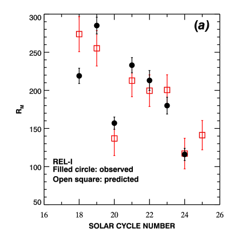
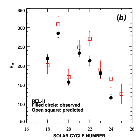
Figure 8: Hindsight: Comparison of the observed and the predicted values of $R_{\rm M}$ of Solar Cycles 18 – 24. The predictions are made by using (a) REL-I and (b) REL-II. The predicted values of $R_{\rm M}$ of Solar Cycle 25 are also shown.

We checked the reliability of the revised REL-I and REL-II. Figs. 8a and 8b show the observed values of $R_{\rm M}$ of Solar Cycles 18 – 24 and the predictions were made by using REL-I and REL-II, respectively. In these figures we have also shown the predicted values of $R_{\rm M}$ of Solar Cycle 25. As can be seen in Fig. 8a except for Solar Cycle 18, remaining all solar cycles the predicted values closely agree with the corresponding observed values. We don’t know why we obtained the incorrect value for Solar Cycle 18 (any way poor statistics, i.e. only 5 data points). There is also some concern about reliability of $T^{*}_{\rm M}$ because it is considerably small (about 5 months only). However, it contains a reasonably large amount of data (see Table 3). Therefore, the consistency of REL-I seems to be not bad. Hence, the prediction for Solar Cycle 25 that made by using REL-I seems to be reasonably reliable and we believe that by using this relation a reasonable good prediction could also be made in future for an upcoming solar cycle. As can be seen in Fig. 8b, the predicted values of Solar Cycles 22 and 24 do not agree with the corresponding observed values. Remaining all other cycles the agreement is good. Hence, the prediction for Solar Cycle 25 seems to be also reasonably reliable, but by using REL-II a reasonable good prediction may be possible mostly only for an odd-numbered solar cycle.

3.3 130-year periodicity in solar activity and similar solar cycles

The extrapolation of a cosine fit to the amplitudes of Solar Cycles 12 – 24 indicated that Solar Cycle 25 will be slightly larger than the weak Solar Cycle 24 (Javaraiah, 2022, 2023). A number of authors predicted the Dalton minimum like low level of activity around Solar Cycle 25 (e.g., Komitov, 2019; Coban et al., 2021). Du (2020a) found that Solar Cycles 24, 15, 12, 14, 17, and 10 (in that order) are most similar cycles to Solar Cycle 25 (note that this list is not containing Solar Cycle 13) and predicted $137.8\pm 31.3$ for the amplitude of Solar Cycle 25, which is larger than the amplitude of Solar Cycle 24. The cosine fit to the amplitudes of Solar Cycles 12 – 24 suggested that there exists a $\approx$130-year long-term cycle in the amplitude modulation (Javaraiah, 2022, 2023). In view of this and the relative strengths of the amplitudes of solar cycles inferred from the patterns of the ratio $R_{\rm M}/R_{A}$ above, we can expect that the pattern of Solar Cycle 25 may be similar to that of Solar Cycle 13.

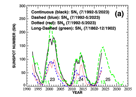
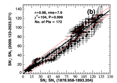
Figure 9: (a) Variations in the 13-month smoothed monthly mean $SN_{\rm T}$, $SN_{\rm N}$, $SN_{\rm S}$, during the period July/1992 – May/2023. The corresponding Waldmeier solar cycles numbers are shown. Variations in the 13-month smoothed monthly mean $SN_{\rm T}$ during the period July/1862 – December/1902 is also shown by forward shifting the epochs by 130-years. (b) Correlation between the $SN_{\rm T}$ during the period 1878.958 – 1893.204 and the $SN_{\rm T}$ during the period 2009.123 – 2023.371. The horizontal and vertical error bars represent the errors in $SN_{i}$ and $SN^{\prime}_{i}$, where $i=1$,…,172, i.e. the errors in the values of $SN_{\rm T}$ of the former and latter periods, respectively. The continuous line represents the best-fit linear relation. The dotted curves are drawn at 1$\sigma$ level. The values of the correlation coefficient ($r$), $\chi^{2}$ and the corresponding probability ($P$), and the number of data points are also shown.

Fig. 9a shows the variations in the 13-month smoothed monthly mean values of $SN_{\rm T}$ and the corresponding values of northern hemisphere ($SN_{\rm N}$) and southern hemisphere ($SN_{\rm S}$), during the period July/1992 – May/2023 (taken from www.sidc.be/silso/datafiles). Variation in the 13-month smoothed monthly mean $SN_{\rm T}$ during the period July/1862 – December/1902, i.e. this period included Solar Cycles 11, 12, and 13, is also shown by shifting the corresponding epochs by 130-years (130-year is added to the epochs). As can be seen in this figure the shape of the whole Solar Cycle 24 and the rising phase of Solar Cycle 25 (for which the data are available) very closely resemble with the shape of Solar Cycle 12 and the rising phase of Solar Cycle 13, respectively. However, the shapes of Solar Cycles 11 and 23 do not match each other well, particularly there exits no match between the maxima of these cycles. The variations in $SN_{\rm N}$ and $SN_{\rm S}$ during Solar Cycles 24 are similar to the variations in the northern and southern hemispheres’ 13-month smoothed monthly mean areas of sunspot groups during Solar Cycle 12 shown in Fig. 1 of Javaraiah (2019, 2020) and also see Fig. 7 in Veronig et al. (2021). Fig. 9b shows the correlation between the $SN_{\rm T}$ during the period 1878.958 – 1893.204 (included full Solar Cycle 12 and the rising phase of Solar Cycle 13) and the $SN_{\rm T}$ during the period 2009.123 – 2023.371 (included full Solar Cycle 24 and the rise phase of Solar Cycle 25). We determined linear least-square-fit to these data. To obtain insignificant $\chi^{2}$ the latter time series is shifted backward with respect to the former by two-months (approximate).

Let $SN_{i}$ is the value of $SN_{\rm T}$ at an epoch $t_{i}$ in the interval 1878.958 – 1893.204 and $SN^{\prime}_{i}$ is the value of $SN_{\rm T}$ at an epoch $t^{\prime}_{i}$ in the interval 2009.123 – 2023.371, where $i=1$,…,172, then obviously

$$t^{\prime}_{i}=t_{i}+130+\frac{2}{12},$$ (8)

and we obtained the linear relation:

$$SN^{\prime}_{i}=SN_{i}(0.919\pm 0.017).$$ (9)

This linear equation is forced to pass through the origin because $SN_{\rm T}$ is never less than zero (the intercept was found to be $-4.34\pm 1.31$). The values of the correlation coefficient ($r$), $\chi^{2}$ and the corresponding probability ($P$), and the number of data points are also shown in Fig. 9b. Uncertainties of both the abscissa and ordinate are taken care in the calculation of the least-square-fit. This linear relation (Eq. (9)) is reasonably accurate, i.e. the value of $r$ is high and the value of $\chi^{2}$ is reasonably small (the value of $P$ is high) and moreover the ratio (equal to 54) of the slope to its standard division is very high.

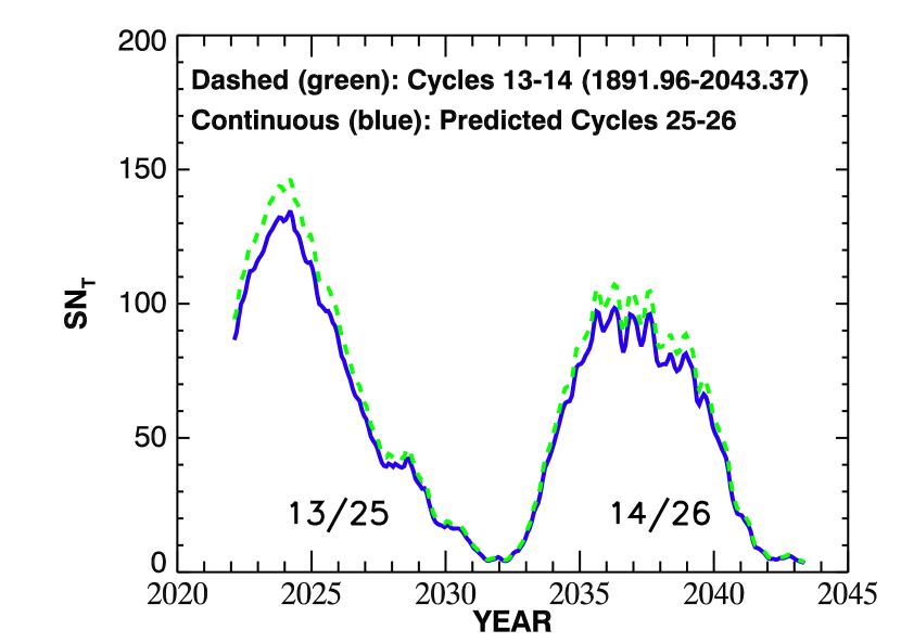
Figure 10: Variations in the predicted 13-month smoothed monthly mean $SN_{\rm T}$ during Solar Cycles 25 – 26, obtained by using Eqs. (8) and (9) and the time series of 13-month smoothed monthly mean $SN_{\rm T}$ during Solar Cycles 13 – 14. The variation in $SN_{\rm T}$ during Solar Cycles 13 – 14 is also shown.

Fig. 10 shows variations in the predicted 13-month smoothed monthly mean $SN^{\prime}_{\rm T}$ during Solar Cycles 25 – 26, determined by using Eqs. (8) and (9) and the time series of 13-month smoothed monthly mean $SN_{\rm T}$ of Solar Cycles 13 – 14. In this figure the variation in the $SN_{\rm T}$ during Solar Cycles 13 – 14 is also shown. As we can see in this figure there exists a remarkable matching between the curves of the predicted Solar Cycles 25 – 26 and Solar Cycles 13 – 14 in most of the times except during the maxima of the solar cycles. Obviously, the maximum and minimum epochs of the predicted Solar Cycles 25 – 26 are simply the values of the maximum and minimum epochs of Solar Cycles 13 – 14 added by 130-year and 2-months (Eq. (8)). The amplitudes of the simulated Solar Cycles 25 – 26 are to some extent lower (about 8 %) than the amplitudes of Solar Cycles 13 – 14. By using the Eq. (9) it seems we are getting a slight (about 8 %) underestimate for $SN^{\prime}_{i}$, i.e. for the predicted $SN_{\rm T}$. Note that these simulations for Solar Cycles 25 – 26 are based on about one-and-half solar cycles data (172 months) are used to derive Eq. (9). In principle by using Eqs. (8) and (9) one can simulate the shapes of several upcoming solar cycles. However, some more cycles data are required to make better simulations/predictions for more solar cycles. On the other hand, the predictions based on the extrapolated methods seem to be less impressive (Petrovay, 2020). The shape of Solar Cycle 23 does not match well with that of Solar Cycle 11. The 130-year period of sunspot activity was found from the limited (13 solar cycles) data. Although it seems to be reasonably reliable because the existence of a $130\pm 0.9$-year periodicity is found from a very large data (9400-year records) of ${}^{14}C$ and ${}^{10}Be$ (McCracken et al., 2013), here we can make prediction for one solar cycle with a reasonable accuracy or tentatively at most two solar cycles. Therefore, in Fig.10 we have shown the predictions for only the two solar cycles, 25 and 26. We obtained $135\pm 8$ for the amplitude of Solar Cycle 25 and 2024.21 (March 2024) for the corresponding maximum epoch. The end of this cycle may occur in 2032.21 (March 2032) with the value $\approx$4 of $SN_{\rm T}$ (minimum value of Solar Cycle 26). These epochs have uncertainties by about 6-months (note that we have used 13-month smoothed monthly mean $SN_{\rm T}$ time series). Solar Cycle 26 would be considerably smaller than Solar Cycle 25. Overall we can conclude that the shape of Solar Cycle 25 will be mostly similar to that of Solar Cycle 13. The amplitude of Solar Cycle 25 will be considerably smaller than the average value 178.7 of the amplitudes of Solar Cycles 1 – 24 (Pesnell, 2018) and the corresponding maximum would occur in March/2024 ($\pm$ 6-month) and the Solar Cycle 25 will end in March/2032 ($\pm$6-month). The length of Solar Cycle 25 will be about 12-year, i.e. Solar Cycle 25 would be a long and below average size solar cycle and will be followed by the weak Solar Cycle 26 (weakest in 12 - 13 decades).

A number of authors predicted a weak-moderate Solar Cycle 25 but stronger than Solar Cycle 24 (e.g., Cameron et al., 2016; Okoh et al., 2018; Pesnell and Schatten, 2018; Petrovay et al., 2018; Du, 2020a, b, 2022; Kakad et al., 2020; Kumar et al., 2021, 2022; Javaraiah, 2008, 2022; Lu et al., 2022; Zhu et al., 2022; Brajša et al., 2022; Nagovtsyn and Ivanov, 2023; Luo and Tan, 2024). Our prediction here is consistent with these. Many authors predicted that maximum of Solar Cycle 25 will take place in 2025 (e.g., Pesnell and Schatten, 2018; Okoh et al., 2018; Labonville et al., 2019; Javaraiah, 2019). However, it has been also predicted that the maximum peak of this cycle will take place in 2024 (Singh and Bhargawa, 2017; Bhowmik, 2018; Petrovay et al., 2018; Li et al., 2018; Du, 2020a; Ahluwalia, 2022; Jaswal, et al., 2023; Luo and Tan, 2024). Recently, Jha and Upton (2024) in their advective flux transport model assumed the activity during Solar Cycle 25 will be similar to that of during Solar Cycle 13 and predicted the peak of Solar Cycle 25 will occur between April and August of 2024. Our prediction here is almost the same as this. Lu et al. (2022) by using a bi-modal forecasting model predicted that Solar Cycle 25 will be single-peak structure and the peak will occur in October/2024. From a method of similar cycles Du (2020a) has predicted that a secondary peak in Solar Cycle 25 will occur eight-months earlier than the major peak. As in the case of Solar Cycle 13 (e.g., Javaraiah, 2023), in Solar Cycle 25 the second peak may be the main peak and would occur about one-year after the first peak (secondary peak), but the ratio of the value of the first peak to that of the second peak would be large ($\approx$0.95). The first peak of Solar Cycle 25 might have been already occurred and could not be clearly seen in the time series of 13-month smoothed monthly mean $SN_{\rm T}$ (on the other hand the current level of the rising phase may represent the first peak).

4 Discussion and conclusions

Here we analysed the combined data of sunspot groups from GPR during the period 1874 – 1976 and DPD during the period 1977 – 2017 and determined the monthly mean, annual mean, and 13-month smoothed monthly mean whole sphere sunspot-group area (WSGA). We have also analysed the monthly mean, annual mean, and 13-month smoothed monthly mean version 2 of international sunspot number ($SN_{\rm T}$) during the period 1874 – 2017. We determined correlation between WSGA and $SN_{\rm T}$ and found that the statistical significance of the correlation is good in each solar cycle. We fitted the annual mean WSGA and $SN_{\rm T}$ data during each of Solar Cycles 12 – 24 separately to the linear and nonlinear (parabola) forms. In the cases of Solar Cycles 14, 17, and 24 the nonlinear fits are found better than the corresponding linear fits. We find that there exists a secular decreasing trend in the slope of the WSGA–$SN_{\rm T}$ linear relation during Solar Cycles 12 – 24, superimposed on it a weak $\approx 77$-year variation. The slope of the average Solar Cycle 15 is found to be largest and is at about 95 % confidence level. A secular decreasing trend is also seen in the coefficient of the first order term of the nonlinear relation. There is no significant correlation between the slope/coefficient and the amplitude of a solar cycle. The cycle-to-cycle variation in the ratio of the amplitude ($R_{\rm M}$) of a solar cycle to the value ($R_{A}$) of WSGA at the maximum epoch of the solar cycle is found to be very during Solar Cycles 12 – 24 and closely similar to that of the slope. The existence of $\approx 77$-year long-term variation in this ratio $R_{\rm M}/R_{A}$ is seen clearly (amplitude is equal to $\approx 2\sigma$). Based on this long-term variation of the ratio we predicted that: Solar Cycle 25 is larger than the small Solar Cycle 24 but its amplitude would be smaller than the average value of the amplitudes of Solar Cycles 1 – 24, Solar Cycle 26 would be smaller than Solar Cycle 25, and the solar cycle pair (26, 27) will satisfy the Gnevyshev-Ohl rule or G-O rule of solar cycles, and Solar Cycle 28 will be smaller than Solar Cycle 27. Using an our earlier method (now slightly revised), i.e. using high correlations of the amplitude of a solar cycle with the sums of the areas of sunspot groups in $0$ – $10^{\circ}$ latitude intervals of the northern hemisphere during 3.75-year interval around the minimum–and the southern hemisphere during 0.4-year near the maximum–of the corresponding preceding solar cycle, we predicted the values $127\pm 26$ and $141\pm 19$ for the amplitude of Solar Cycle 25, respectively. Based on the existence of $\approx$130-year periodicity in the cycle-to-cycle variation of the amplitudes of Solar Cycles 12 – 24 (Javaraiah, 2022, 2023) we find the shape of Solar Cycle 25 would be similar to that of Solar Cycle 13 and predicted $135\pm 8$ for the amplitude of Solar Cycle 25, 2024.21 (March 2024)$\pm$6-month for the corresponding maximum epoch, and ending in 2032.21 (March 2032)$\pm$ 6-month with the value $\approx 4$ of $SN_{\rm T}$ (minimum value of Solar Cycle 26). The length of Solar Cycle 25 is expected to $\approx$12-year. The Solar Cycle 26 would be a small cycle and is expected to be similar as that of Solar Cycle 14.

The ratio $R_{\rm M}/R_{A}$ is large in some cycles (15, 21) and small in some other cycles. It indicates that in the former case the ratio of the number of large size sunspot groups to that of the small size sunspot groups may be small, whereas in the latter case this ratio may be large. In the former case while the magnetic structures of sunspot groups rising through the convection zone disintegrate or fragment into more small structures (e.g., Gokhale and Javaraiah, 2002) than in the latter case.

Because of variation in the slopes of the linear relationships of WSGA and $SN_{\rm T}$ of different solar cycles, this analysis also suggest that the prediction made by using the slope of the relationship between WSGA and $SN_{\rm T}$ determined from the data of whole period 1874 – 2017 might have a large uncertainty (Javaraiah, 2021). The corresponding prediction made by using the linear relationship between the logarithm values of WSGA and $SN_{\rm T}$ (Javaraiah, 2023) may be also to some extent erroneous because in the present analysis we also find that the linear-least-square best fits of the logarithm values of WSGA and $SN_{\rm T}$ of individual solar cycles are not well defined. The fit of the logarithm values of WSGA and $SN_{\rm T}$ of the entire period of 1874 – 2017 may be better than the corresponding linear fit of the original values due to the ratio of the number of small size sunspot groups to the number of large size sunspot groups is not the same in all solar cycles (Javaraiah, 2016), may be considerably large in some solar cycles.

A reasonable correlation exists between solar cycle maximum ($R_{\rm M}$) and the preceding minimum (Tlatov, 2009; Hathaway, 2015). But it is not possible to make a precise prediction for the former from the latter (Du and Wang, 2010). However, it seems possible from the 13-month smoothed minimum just after onset of the cycle (Ramesh, 2000; Ramesh and Bhagya Lakshmi, 2012). From this method it seems possible to predict $R_{\rm M}$ of a solar cycle by about three years in advance. From our method, i.e. by using the relation REL-I, the $R_{\rm M}$ of a solar cycle may be possible to predict by nine years in advance and by using REL-II the $R_{\rm M}$ of mostly only an odd-numbered solar cycle may be possible to predict by about thirteen years in advance. It may be worth to note here that the two main ingredients of solar dynamo mechanism, deferential rotation and meridional flow, differ in odd- and even-numbered solar cycles (Javaraiah, 2003, 2008; Javaraiah et al., 2005). As we have already discussed in Javaraiah (2008), equatorial crossing of magnetic flux due to rotation of the Sun on inclined axis could be the reason behind the relations REL-I and REL-II.

Regarding the existence of $\approx$130-year periodicity in the amplitude modulation of solar cycles (Javaraiah, 2022, 2023) that we have used here for finding the similar solar cycles and predicting the repetitions of the patterns of Solar Cycles 12 – 14 in Solar Cycles 24 – 26, the existence of $\approx$130-year periodicity in some solar activity related phenomena are known. Attolini et al. (1990a, b) found the existence of $\approx$22-year, $\approx$88-year (Gleissberg cycle), and $\approx$132-year periodicities in aurorae, ${}^{14}C$ from tree rings, and ${}^{10}Be$ from polar ice and suggested that 1/88-year and 1/132-year frequencies might be two sub-harmonics of the 22-year Hale cycle. According to them these results support the idea that the Sun behaves as nonlinear system forced internally by 22-year torsional magnetohydrodynamic oscillation (Bracewell, 1986, 1988; Gokhale et al., 1992; Gokhale and Javaraiah, 1992, 1995). The required forcing may be also coming from the alignments of Venus, Earth, and Jupiter. These are the tidally dominant planets and whose alignments might have a significant role in the solar cycle mechanism (Wood, 1972; Wilson, 2013; Stefani et al., 2021, and references therein). McCracken et al. (2013) found the existence of a $130\pm 0.9$-year periodicity in 9400-year records of ${}^{14}C$ and ${}^{10}Be$. It may be worth to note that $213V=131E=11J=131$-year, where $V=0.615$-year, $E=1$-year, and $J=11.9$-year, are the orbital periods of Venus, Earth, and Jupiter, respectively. That is, the relative orbital positions (configurations) of these planets vary differently during each of the 12 solar cycles that occur within the 131-year period and the configurations would be similar in every 13th solar cycle. Hence, the influences of these planets on solar activity could be similar during every 13th solar cycle. This may be a reason for the shape of Solar Cycle 24 is similar to that of Solar Cycle 12 and the shape of Solar Cycle 25 is expected to be similar to that of Solar Cycle 13. The basic process involved may be the Sun’s spin-orbit coupling (Gokhale and Javaraiah, 1995; Juckett, 2000, 2003; Javaraiah, 2003, 2005). Beside the configurations of the giant planets, some specific alignments of other planets with the giant planets may also have a role in the Sun’s spin-orbit coupling (Wood and Wood, 1965; Wilson, 2013; Stefani et al., 2021). However, the role of the orbital motions of the planets in solar dynamo is not yet clear (Charbonneau, 2022).

Acknowledgments

The author thanks the anonymous reviewers for very useful comments and suggestions. The author acknowledges the work of all the people who contribute and maintain the GPR and DPD sunspot databases. The sunspot-number data are provided by WDC-SILSO, Royal Observatory of Belgium, Brussels.

Figure 5: (a) The filled circle-continuous curve represents variation in $R_{A}$, i.e. the value of the 13-month smoothed monthly mean area of the sunspot groups (WSGA) in whole-sphere at the maximum epoch of solar cycle and the open circle-dashed curve represents the amplitude ($R_{\rm M}$) of solar cycle, during Solar Cycles 12 – 24. (b) Solar cycle-to-cycle variation of the ratio $R_{\rm M}/R_{A}$ (square-continuous curve). The horizontal line represents the mean value (0.0936) of $R_{\rm M}/R_{A}$ over Solar Cycles 12 – 24.

Figure 6: (a) Plot of the amplitude ($R_{\rm M}$, i.e. the largest 13-month smoothed monthly mean $SN_{\rm T}$) of a solar cycle and the sum of the areas ($A^{*}_{\rm M}$) of the sunspot groups in $0$ – $10^{\circ}$ latitude interval of the Sun’s southern hemisphere during the interval ($T^{*}_{\rm M}$) around the maximum epoch ($T_{\rm M}$) of the solar cycle versus the solar cycle number ($n$). (b) The scatter plot of $A^{*}_{\rm M}$ of a Solar Cycle $n$ and $R_{\rm M}$ of Solar Cycle $n+1$. The continuous line represents the corresponding best-fit linear relation REL-I (Eq. (6)) and the dotted lines are drawn at one-rms level. The values of the correlation coefficient ($r$) is also shown. The filled-square represents the predicted value $141\pm 19$ of $R_{\rm M}$ of Solar Cycle 25.

Figure 7: (a) Plot of the amplitude ($R_{\rm M}$) of a solar cycle and the sum of the areas ($A^{*}_{\rm m}$) of the sunspot groups in $0$ – $10^{\circ}$ latitude interval of the Sun’s northern hemisphere during the interval ($T^{*}_{\rm m}$) around the minimum epoch ($T_{\rm m}$) of the solar cycle versus the solar cycle number ($n$). (b) The scatter plot of $A^{*}{\rm{}_{m}}$ of a Solar Cycle $n$ and $R_{\rm M}$ of Solar Cycle $n+1$. The continuous line represents the corresponding best-fit linear relation REL-II (Eq. (7)) and the dotted lines are drawn at one-rms level. The values of the correlation coefficient ($r$) is also shown. The filled-square represents the predicted value $127\pm 26$ of $R_{\rm M}$ of Solar Cycle 25.

Table 1: Values of the slope ($m$) and its uncertainty ($\sigma_{m}$) of the best fit linear relation (Eq. (1)) of the annual mean values of WSGA and $SN_{\rm T}$ of a solar cycle (SC). The values of $\chi^{2}$ and the corresponding probability ($P$), the ratio $m/\sigma_{m}$, correlation coefficient ($\rm r$), and the number of data points (N) are given. The symbol ^a indicates the incomplete data of Solar Cycle 24. The values of the amplitude ($R_{\rm M}$) of a solar cycle and the value of ($R_{A}$) of WSGA at the epoch of $R_{\rm M}$ and the corresponding uncertainties $\sigma_{R}$ and $\sigma_{A}$, respectively, are also given.

SC	$R_{\rm M}$	$\sigma_{R}$	$R_{A}$	$\sigma_{A}$	$m$	$\sigma_{m}$	$m/\sigma_{m}$	$\chi^{2}$	$P$	$\rm r$	N
12	124.4	12.5	1370.7	121.7	0.101	0.006	16.83	5.27	0.87	0.99	12
13	146.5	10.8	1616.0	109.9	0.099	0.005	19.80	9.73	0.46	0.99	12
14	107.1	9.2	1043.9	139.5	0.101	0.005	20.20	11.77	0.23	0.97	11
15	175.7	11.8	1535.4	170.5	0.111	0.005	22.20	7.06	0.53	0.99	10
16	130.2	10.2	1324.0	122.9	0.089	0.005	17.80	6.57	0.58	0.99	10
17	198.6	12.6	2119.5	175.7	0.097	0.004	24.25	11.51	0.24	0.99	11
18	218.7	10.3	2641.4	209.7	0.084	0.003	28.00	9.62	0.29	0.99	10
19	285.0	11.3	3441.4	208.2	0.085	0.002	42.50	24.88	0.00	0.99	10
20	156.6	8.4	1556.3	81.8	0.088	0.003	29.33	6.84	0.74	0.99	12
21	232.9	10.2	2121.2	161.9	0.098	0.003	32.67	16.94	0.03	0.98	10
22	212.5	12.7	2268.7	193.4	0.084	0.003	28.00	8.51	0.39	0.99	10
23	180.3	10.8	2157.3	205.6	0.083	0.003	27.67	6.92	0.73	$\approx 1$	12
24a	116.4	8.2	1599.8	115.9	0.081	0.004	20.25	14.83	0.06	0.97	10
Whole					0.090	0.001	90.00	249.80	0.00	0.98	144

Table 2: Values of the coefficients ($m_{1}$ and $m_{2}$) and their uncertainties ($\sigma_{m_{1}}$ and $\sigma_{m_{2}}$) of the best fit nonlinear relation (Eq. (2)) of the annual mean values of WSGA and $SN_{\rm T}$ of a solar cycle (SC). The values of ratios $m_{1}/\sigma_{m_{1}}$ and $m_{2}/\sigma_{m_{2}}$ and the values of $\chi^{2}$ and the corresponding probability ($P$) are also given. The symbol ^a indicates the incomplete data of Solar Cycle 24.

SC	$m_{1}$	$\sigma_{m_{1}}$	$m_{2}$	$\sigma_{m_{2}}$	$m_{1}/\sigma_{m_{1}}$	$m_{2}/\sigma_{m_{2}}$	$\chi^{2}$	$P$
12	0.129	0.021	$-2.90\times 10^{-5}$	$2.12\times 10^{-5}$	6.14	$-1.37$	13.40	0.20
13	0.105	0.014	$-5.53\times 10^{-6}$	$1.10\times 10^{-5}$	7.50	$-0.50$	23.23	0.01
14	0.146	0.016	$-4.71\times 10^{-5}$	$1.53\times 10^{-5}$	9.12	$-3.08$	3.42	0.97
15	0.102	0.012	$8.25\times 10^{-6}$	$1.03\times 10^{-5}$	8.50	$0.80$	6.74	0.57
16	0.106	0.018	$-1.39\times 10^{-5}$	$1.38\times 10^{-5}$	5.89	$-1.01$	10.42	0.32
17	0.124	0.012	$-1.53\times 10^{-5}$	$6.19\times 10^{-6}$	10.33	$-2.47$	5.99	0.82
18	0.098	0.009	$-6.31\times 10^{-6}$	$4.01\times 10^{-6}$	10.89	$-1.57$	14.50	0.11
19	0.109	0.007	$-9.09\times 10^{-6}$	$2.42\times 10^{-6}$	15.57	$-3.76$	9.66	0.29
20	0.100	0.011	$-8.12\times 10^{-6}$	$6.87\times 10^{-6}$	9.09	$-1.18$	43.41	0.00
21	0.093	0.012	$2.13\times 10^{-6}$	$5.81\times 10^{-6}$	7.75	$0.37$	19.85	0.02
22	0.104	0.010	$-9.00\times 10^{-6}$	$4.48\times 10^{-6}$	10.40	$-2.01$	11.71	0.23
23	0.087	0.009	$-1.96\times 10^{-6}$	$4.70\times 10^{-6}$	9.66	$-0.42$	8.10	0.70
24a	0.111	0.009	$-2.51\times 10^{-5}$	$6.97\times 10^{-6}$	12.33	$-3.60$	4.16	0.84
Whole	0.103	0.002	$-7.14\times 10^{-6}$	$1.04\times 10^{-6}$	51.50	$-6.86$	296.88	0.00

Table 3: $T_{\rm M}$ and $T_{\rm m}$ are the maximum and minimum epochs of a solar cycle ($n$). $A^{*}_{\rm M}$ and $A^{*}_{\rm m}$ represent the sums of the areas (msh) of the sunspot groups (normalized by 1000) in $0^{\circ}-10^{\circ}$ latitude intervals of the southern and northern hemispheres during the time intervals $T^{*}_{\rm M}=0.4$-year near $T_{\rm M}$ (i.e., $T^{*}_{\rm M}+1.2$-year – $T^{*}_{\rm M}+1.6$-year) and $T^{*}_{\rm m}=3.75$-year around $T_{\rm m}$ (i.e., $T_{\rm m}-1.4$-year – $T_{\rm m}+2.35$-year) of a solar cycle, respectively. The symbol ^b indicates that the epochs of the first peaks are used (see the text).

$n$	$T_{\rm M}$	$T^{*}_{\rm M}$	$A^{*}_{\rm M}$	$T_{\rm m}$	$T^{*}_{\rm m}$	$A^{*}_{\rm m}$
12	1883.96	1885.16-1885.56	19.75	1878.96	1877.56-1881.31	10.86
13	1894.04	1895.24-1895.64	19.00	1890.20	1888.80-1892.55	11.62
14	1906.12	1907.32-1907.72	25.76	1902.04	1900.64-1904.39	11.77
15	1917.62	1918.82-1919.22	28.19	1913.62	1912.22-1915.97	9.79
16	1928.29	1929.49-1929.89	33.07	1923.62	1922.22-1925.97	36.47
17	1937.29	1938.49-1938.89	54.28	1933.71	1932.31-1936.06	37.48
18	1947.37	1948.57-1948.97	65.21	1944.12	1942.72-1946.47	69.91
19	1958.20	1959.40-1959.80	22.78	1954.29	1952.89-1956.64	23.93
20	1968.87	1970.07-1970.47	45.93	1964.79	1963.39-1967.14	54.42
21	1979.96	1981.16-1981.56	40.56	1976.21	1974.81-1978.56	65.30
22	1989.87	1991.07-1991.47	40.52	1986.71	1985.31-1989.06	35.06
23	2000.29b	2001.49-2001.89	14.55	1996.62	1995.22-1998.97	24.84
24	2012.21b	2013.41-2013.81	22.33	2008.96	2007.56-2011.31	10.93

References

- Ahluwalia (2022) Ahluwalia, H.S., 2022. Forecast for sunspot cycle 25 activity. Adv. Space Res. 69, 794. 10.1016/j.asr.2021.09.035.
- Attolini et al. (1990a) Attolini, M.R., Cecchini, S., Galli, M., Nanni, T., 1990a. The subharmonics of the 22-year solar cycle. NCimC. 13, 131. 10.1007/BF02515782.
- Attolini et al. (1990b) Attolini, M.R., Cecchini, S., Galli, M., Nanni, T., 1990b. On the persistence of the 22-YEAR solar cycle. Solar Phys. 125, 389. 10.1007/BF00158414.
- Bhowmik (2018) Bhowmik, P., Nandy, D., 2018. Prediction of the strength and timing of sunspot cycle 25 reveal decadal-scale space environmental conditions. Nat. Commun. 9, 5209. 10.1038/s41467-018-07690-0.
- Bracewell (1986) Bracewell, R.N., 1986. Simulating the sunspot cycle. Nature 323, 516. 10.1038/323516a0.
- Bracewell (1988) Bracewell, R.N., 1988. Three-halves law in sunspot cycle shape. Mon. Not. Roy. Astron. Soc. 230, 535. 10.1093/230.4.535.
- Brajša et al. (2022) Brajša. R., Verbanac, G., Bandić, M., Hanslmeier, A., Skokić, I., Sudar, D., 2022. A prediction for the 25th solar cycle maximum amplitude. AN, 343, e13960. 10.1002/asna.202113960.
- Cameron et al. (2016) Cameron, R.H., Jiang, J., Schüssler, M., 2016. Solar cycle 25: Another moderate cycle? Astrophys. J. Lett. 823, l22. 10.3847/2041-8205/823/2/L22.
- Charbonneau (2022) Charbonneau, P., 2022. External Forcing of the Solar Dynamo. Front. Astron. Space Sci. 9, 853676. 10.3389/fspas.2022.853676.
- Clette and Lefévre (2016) Clette, F., Lefévre, L., 2016. The new sunspot number: Assembling all corrections. Solar Phys. 291, 2629.10.1007/s11207-016-1014-y.
- Coban et al. (2021) Coban, G.C., Raheem, A., Cavus, H., Asghan-Targhi, M., 2021. Can solar cycle 25 be a new Dalton minimum? Solar Phys. 296, 156. 10.1007/s11207-021-01906-1
- Dikpati, et al. (2008) Dikpati, M., Gilman, P. A., de Toma, G., 2008. The Waldmeier effect: An artifact of the definition of wolf sunspot number? Astrophys. J. Lett. 673, L99. 10.1086/527360.
- Du (2020a) Du, Z., 2020a. Predicting the shape of solar cycle 25 using a similar-cycle method. Solar Phys. 295, 134. 10.1007/s11207-020-01701-4.
- Du (2020b) Du, Z., 2020b. Predicting the amplitude of solar cycles 25 using the value 39 months before the solar minimum. Solar Phys. 295, 147. 10.1007/s11207-020-01720-1.
- Du (2022) Du, Z., 2022. Predicting the amplitude of solar cycle 25 using the early value of the rising phase. Solar Phys. 297, 61. 10.1007/s11207-022-01991-w.
- Du and Wang (2010) Du, Z.L., Wang, H.N., 2010. Does a low solar cycle minimum hint at a weak upcoming cycle? Res. in Astron. and Astrophys. 10, 950. 10.1088/1674-4527/10/10/002.
- Gnevyshev and Ohl (1948) Gnevyshev, M.N., Ohl, A.I., 1948. About 22-year cycle of solar activity. AZh 25, 18.
- Gokhale and Javaraiah (1992) Gokhale, M.H., Javaraiah, J., 1992. Global modes constituting the solar magnetic cycle - Part Two. Solar Phys. 138, 399. 10.1007/BF00151923.
- Gokhale and Javaraiah (1995) Gokhale, M.H., Javaraiah, J., 1995. Global modes constituting the solar magnetic cycle - Part Three. Solar Phys. 156, 157. %****␣number-area-rv2-clean.tex␣Line␣1025␣****10.1007/BF00669582.
- Gokhale and Javaraiah (2002) Gokhale, M.H., Javaraiah, J. in J. Javaraiah and M.H. Gokhale (eds), The Sun’s rotation, Nova Science, New York, pp.109, 2002.
- Gokhale et al. (1992) Gokhale, M.H., Javaraiah, J. Narayanakutty, K., Varghese, B.A., 1992. Global modes constituting the solar magnetic cycle - Part One. Solar Phys. 138, 35. 10.1007/BF00146195.
- Hathaway (2015) Hathaway, D.H., 2015. The Solar Cycle. Liv. Rev. Solar. Phys. 12, 4. 10.1007/1rsp-2015-4.
- Hathaway et al. (2002) Hathaway, D.H., Wilson, R.M., Reichmann, E.J., 2002. Group sunspot numbers; sunspot cycle characteristics. Solar Phys. 211, 357. 10.1023/A:1022425402664.
- Jaswal, et al. (2023) Jaswal, P., Saha, C., Nandy, D., 2023. Discovery of a relation between the decay rate of the Sun’s magnetic dipole and the growth rate of the following sunspot cycle: a new precursor for solar cycle prediction. Mon. Not. Roy. Astron. Soc. 528, L27. 10.1093/mnrasl/slad122.
- Javaraiah (2003) Javaraiah, J., 2003. Long–term variations in the solar differential rotation. Solar Phys. 212, 23. DOI: 10.1023/A:1022912430585.
- Javaraiah (2005) Javaraiah, J., 2005. Sun’s retrograde motion and violation of even-odd cycle rule in sunspot activity. Mon. Not. Roy. Astron. Soc. 362, 1311. 10.1111/j.1365-2966.2005.09403.x.
- Javaraiah (2007) Javaraiah, J., 2007. North–south asymmetry in solar activity: predicting the amplitude of the next solar cycle. Mon. Not. Roy. Astron. Soc. 377, L34. 10.1111/j.1745-3933.2007.00298.x.
- Javaraiah (2008) Javaraiah, J., 2008. Predicting the amplitude of a solar cycle using the north–south asymmetry in the previous cycle: II. An improved prediction for solar cycle 24. Solar Phys. 252, 419. 10.1007/s11207-008-9269-6.
- Javaraiah (2012) Javaraiah, J., 2012. The G–O rule and Waldmeier effect in the variations of the numbers of large and small sunspot groups. Solar Phys. 281, 827. 10.1007/s11207-012-0106-6.
- Javaraiah (2015) Javaraiah, J., 2015. Long–term variations in the north–south asymmetry of solar activity and solar cycle prediction, III: Prediction for the amplitude of solar cycle 25. NewA 34, 54. 10.1016/j.newast.2014.04.001.
- Javaraiah (2016) Javaraiah, J., 2016. North-south asymmetry in small and large sunspot group activity and violation of even-odd solar cycle rule. Astrophys. Space Sci. 361, 208. 10.1007/s10509-016-2797-x.
- Javaraiah (2017) Javaraiah, J., 2017. Will solar cycles 25 and 26 be weaker than cycle 24? Solar Phys. 292, 172. 10.1007/s11207-017-1197-x.
- Javaraiah (2019) Javaraiah, J., 2019. North–south asymmetry in solar activity and solar cycle prediction, IV: Prediction for lengths of upcoming solar cycles. Solar Phys. 294, 64. 10.1007/s11207-019-1442-6.
- Javaraiah (2020) Javaraiah, J., 2020. Long–term periodicities in north–south asymmetry of solar activity and alignments of the giant planets. Solar Phys. 295, 8. 10.1007/s11207-019-1575-7.
- Javaraiah (2021) Javaraiah, J. 2021. North–south asymmetry in solar activity and solar cycle prediction, V: Prediction for the north–south asymmetry in the amplitude of Solar Cycle 25. Astrophys. Space Sci. 366, 16. 10.1007/s10509-021-03922-w.
- Javaraiah (2022) Javaraiah, J., 2022. Long-term variations in solar activity: Predictions for amplitude and north–south asymmetry of solar cycle 25. Solar Phys. 297, 33. 10.1007/s11207-022-01956-z.
- Javaraiah (2023) Javaraiah, J., 2023. Prediction for the amplitude and second maximum of Solar Cycle 25 and a comparison of the predictions based on strength of polar magnetic field and low-latitude sunspot area. Mon. Not. Roy. Astron. Soc. 520, 5586. 10.1093/mnrasl/stad479.
- Javaraiah et al. (2005) Javaraiah, J., Bertello, L., Ulrich, R.K., 2005. An interpretation of the differences in the solar differential rotation during even and odd sunspot cycles. Astrophys. J. 626, 579. 10.1086/429898.
- Jha and Upton (2024) Jha, B.K., Upton, L.A., 2024. Predicting the timing of the Solar Cycle 25 polar field reversal. Astrophys. J. Lett. 962, L15. 10.3847/2041-8213/ad20d2.
- Juckett (2000) Juckett, D.A., 2000. Solar activity cycles, North/South asymmetries, and differential rotation associated with solar spin-orbit variations. Solar Phys. 191, 201. 10.1023/A:1005226724316.
- Juckett (2003) Juckett, D., 2003. Temporal variations of low-order spherical harmonic representations of sunspot group patterns: Evidence for solar spin-orbit coupling. Astron. Astrophys. 399, 731. 10.1051/0004-6361:20021923.
- Kakad et al. (2020) Kakad, B., Kumar, R., Kakad, A., 2020. Randomness in sunspot number: A clue to predict solar cycle 25. Solar Phys. 295, 88. 10.1007/s11207-020-01655-7.
- Karak and Choudhuri (2011) Karak, B.B., Choudhuri, A.R., 2011. The Waldmeier effect and the flux transport solar dynamo. Mon. Not. Roy. Astron. Soc. 410, 1503. 10.1111/j.1365-2966.2010.17531.x.
- Kilcik et al. (2011) Kilcik, A., Yurchyshyn, V.B., Abramenko, V., Goode, P.R., Ozguc, A., Rozelot, J.P., Cao, W., 2011. Time distribution of large and small sunspot groups over four solar cycles. Astrophys. J. 731, 30. 10.1088/0004-637X/731/1/30.
- Komitov (2019) Komitov, B., 2019. The 24th solar cycle: Preliminary analysis and generalizations. BlgAJ 30, 3.
- Kumar et al. (2022) Kumar, P., Biswas, A., Karak, B.B., 2022. Physical link of the polar field buildup with the Waldmeier effect broadens the scope of early solar cycle prediction: Cycle 25 is likely to be slightly stronger than Cycle 24. Mon. Not. Roy. Astron. Soc. 513, L112. 10.1093/mnrasl/slac043.
- Kumar et al. (2021) Kumar, P., Nagy, M., Lemerle, A., Karak, B.B., Petrovay, K. 2021. The polar precursor method for solar cycle prediction: Comparison of predictors and their temporal range. Astrophys. J. 909, 87. 10.3847/1538-4357/abdbb4.
- Labonville et al. (2019) Labonville, F., Charbonneau, P., Lemerle, A., 2019. A Dynamo-based forecast of solar cycle 25. Solar Phys. 294, 82. 10.1007/s11207-019-1480-0.
- Li et al. (2018) Li, F.Y., Kong, D.F., Xie, J.L., Xiang, N.B., Xu, J.C., 2018. Solar cycle characteristics and their application in the prediction of cycle 25. J. Atmos. Solar-Terr. Phys. 181, 110. 10.1016/j.jastp.2018.10.014.
- Lu et al. (2022) Lu, J.Y., Xiong, Y.T., Zhao, K., Wang, M., Li, J.Y., Peng, G.S., Sun, M., 2022. A Novel Bimodal Forecasting Model for Solar Cycle 25. Astrophys. J. 924, 59. 10.3847/1538-4357/ac3488.
- Luo and Tan (2024) Luo, P-X., Tan, B-L., 2024. Long-term evolution of solar activity and prediction of the following solar cycles. Res. in Astron. and Astrophys. 24, 035016 (11pp). 10.1088/1674-4527/ad1ed2.
- McCracken et al. (2013) McCracken, K.G., Beer, J., Steinhilber, F., Abreu, J., 2013. A Phenomenological study of the cosmic ray variations over the past 9400 years, and their implications regarding solar activity and the solar dynamo. Solar Phys. 286, 609. 10.1007/s11207-013-0265-0.
- Mandal et al. (2016) Mandal, S., Banerjee, D., 2016. Sunspot sizes and the solar cycle: Analysis using Kodaikanal white-light digitized data. Astrophys. J. Lett. 830, L33. 10.3847/2041-8205/830/2/L33.
- Nandy (2021) Nandy, D., 2021. Progress in solar cycle predictions: Sunspot Cycles 24 – 25 in perspective, Solar Phys. 296, 54. 10.1007/s11207-021-01797-2.
- Nagovtsyn and Ivanov (2023) Nagovitsyn, Y.A., Ivanov, V.G., 2023. Solar cycle paring and prediction of cycle 25. Solar Phys. 298, 37. 10.1007/s11207-023-02121-w.
- Okoh et al. (2018) Okoh, D.I., Seemala, G.K., Rabiu, A.B., Uwamahoro, J., Habarulema, J.B., Aggarwal, M., 2018. A hybrid regression-neural network (HR-NN) method for forecasting the solar activity. Space Weather 16, 1424. 10.1029/2018SW001907.
- Pesnell (2012) Pesnell, W.D., 2012. Solar cycle predictions (invited review). Solar Phys. 281, 507. 10.1007/s11207-012-9997-5.
- Pesnell (2018) Pesnell, W.D., 2018. Effects of version 2 of the international sunspot number on naïve predictions of solar cycle 25. Space Weather 16, 1997. 10.1029/2018SW002080.
- Pesnell and Schatten (2018) Pesnell, W.D., Schatten, K.H., 2018. An early prediction of the amplitude of solar cycle 25. Solar Phys. 293, 112. 10.1007/s11207-018-1330-5.
- Petrovay (2020) Petrovay, K., 2020. Solar cycle prediction. Liv. Rev. Solar Phys. 17, 2. 10.1007/s41116-020-0022-z.
- Petrovay et al. (2018) Petrovay, K., Nagy, M., Gerjàk, T., Juhàsz, L., 2018. Precursors of an upcoming solar cycle at high latitudes from coronal green line data. J. Atmos. Solar-Terr. Phys. 176, 15. 10.3103/S0884591308050036.
- Ramesh (2000) Ramesh, K.B., 2000. Dependence of on - a reconsideration for predicting the amplitude of a sunspot cycle. Solar Phys. 197, 421. 10.1023/A:1026565028898.
- Ramesh and Bhagya Lakshmi (2012) Ramesh, K.B., Bhagya Lakshmi, N., 2012. The amplitude of sunspot minimum as a favorable precursor for the prediction of the amplitude of the next solar maximum and the limit of the Waldmeier effect. Solar Phys. 276, 395. 10.1007/s11207-011-9866-7.
- Ramesh and Rohini (2008) Ramesh, K.B., Rohini, V.S., 2008. 1.8 øA, Coronal cackground X-ray emmission and the associated indicators of photospheric magnetic activity. Astrophys. J. Lett. 686, L41. 10.1086/592774.
- Singh and Bhargawa (2017) Singh, A.K., Bhargawa, A., 2017. An early prediction of 25th solar cycle using Hurst exponent. Astrophys. Space Sci. 362, 199. 10.1007/s10509-017-3180-2.
- Stefani et al. (2021) Stefani, F., Stepanov, R., Weler, T., 2021. Shaken and Stirred: When Bond meets Suess–de Vries and Gnevyshev–Ohl. Solar Phys. 296, 88. 10.1007/s11207-021-01822-4.
- Tlatov (2009) Tlatov, A.G., 2009. The minimum activity epoch as a precursor of the solar activity. Solar Phys. 260, 465. 10.1007/s11207-009-9451-5.
- Veronig et al. (2021) Veronig, A.M., Jain, S., Podladchikova,T., Pötzi, W., Clette, F., 2021 Hemispheric sunspot numbers 1874 – 2020. Astron. Astrophys. 652, 56. 10.1051/0004-6361/202141195.
- Wilson (2013) Wilson, I.R.G., 2013. The Venus–Earth–Jupiter spin–orbit coupling model. Pattern Recogn. Phys. 1, 147. 10.1086/508013.
- Wilson and Hathaway (2006) Wilson, R.M., Hathaway, D.H., 2006. On the relation between sunspot area and sunspot number. NASA/STI/Recon. Tech. Rep. No. 6.
- Wood (1972) Wood, K., 1972. Sunspots and planets. Nature 240 (5376), 91. 10.1038/240091a0.
- Wood and Wood (1965) Wood, R.M., Wood, K.D., 1965. Solar motion and sunspot comparison Nature 208, 129. 10.1038/208129a0.
- Zhu et al. (2022) Zhu, H., Zhu, W., He, M., 2022. Prediction using an optimized long short-term memory mode with F10.7. Solar Phys. 297, 157. 10.1007/s11207-022-02091-5.