pyCFS-data: Data Processing Framework in Python for openCFS

Abstract

Many numerical simulation tools have been developed and are on the market, but there is still a strong need for appropriate tools capable of simulating multi-field problems, especially in aeroacoustics. Therefore, openCFS provides an open-source framework for implementing partial differential equations using the finite element method. Since 2000, the software has been developed continuously. The result is openCFS (before 2020, known as CFS++ Coupled Field Simulations written in C++). In this paper, we present pyCFS-data, a data processing framework written in Python to provide a flexible and easy-to-use toolbox to access and manipulate, pre- and postprocess data generated by or for usage with openCFS.

Keywords Data processing framework  $\cdot$ Python  $\cdot$ Open Source FEM Software  $\cdot$ Multiphysics Simulation  $\cdot$ openCFS

1 Introduction

Within this contribution, we concentrate on the pyCFS[1] module pyCFS-data, a data processing framework for openCFS [2]. It consists of three main components, which are organized in same-titled submodules

• io

• operators

• extras

where the io submodule focuses on reading, writing, and accessing data in HDF5 file format as used in openCFS. The operators submodule contains functionality for data pre-, and post-processing based on data structures defined in io submodule. The extras submodule contains methods to interact with data stored in different file formats.

The module can be easily installed, including all dependencies, via the pyPI

⬇

pip install pycfs

Detailed instructions for installation inside a virtual environment and developer setup can be found at https://opencfs.gitlab.io/pycfs/installation.html

When establishing an XML file for CFS-Data, it is fundamental that the pipeline, existing of different CFS-Data filters, is closed. The pipeline has to start with the step value definition and has to be followed by the input filter and end with the output filter. In between, multiple filters can be added, serial or parallel.

In this contribution, we discuss the capability of each submodule of pyCFS-data in more detail. Comprehensive and up-to-date documentation of the library can be found in the pyCFS API Documentation.

2 I/O of openCFS based HDF5 files (io)

2.1 Reader class (CFSReader)

Base class for all reading operations. A simple example of usage could look like the following

⬇

from pyCFS.data.io import CFSReader

with CFSReader(’file.cfs’) as f:

mesh = f.MeshData

results = f.MultiStepData

, which reads the file file.cfs into the data objects mesh and results, containing the description of the computational grid and result data, respectively.

2.2 Writer class (CFSWriter)

Base class for all writing operations. A simple example of usage could look like the following

⬇

from pyCFS.data.io import CFSReader, CFSWriter

with CFSReader(’file_in.cfs’) as f:

mesh = f.MeshData

results = f.MultiStepData

with CFSWriter(’file_out.cfs’) as f:

f.create_file(mesh_data=mesh, result_data=results)

, which reads the file file_in.cfs into the data objects mesh and results, containing the description of the computational grid and result data, respectively. Thereafter, this information is written to a newly created file file_out.cfs.

2.3 Data structures (CFSMeshData,CFSResultData, etc.)

The structure of data is organized as depicted in Fig. 1.

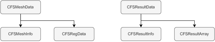
Figure 1: Organization of classes for data structures.

CFSMeshData: Data structure containing mesh definition. Its attributes and properties are depicted in Fig. 2.

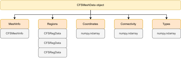
Figure 2: Structure of CFSMeshData class. Attributes are highlighted in orange, Properties in purple, and respective data types in grey.

CFSMeshInfo: Data structure containing mesh information.

CFSRegData: Data structure containing mesh region definition. Its attributes and properties are depicted in Fig. 3.

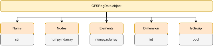
Figure 3: Structure of CFSRegData class. Attributes are highlighted in orange, Properties in purple, and respective data types in grey.

CFSResultData: Data structure containing result data (one object currently supports a single MultiStep only!). Its attributes and properties are depicted in Fig. 4.

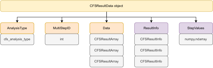
Figure 4: Structure of CFSResultData class. Attributes are highlighted in orange, Properties in purple, and respective data types in grey.

CFSResultArray: Overload/Subclass of numpy.ndarray adding attributes according to CFS HDF5 result data structure. Its additional attributes and properties are depicted in Fig. 5.

Field data can be defined on the nodes or the cell centroids of a computational grid (ResType attribute) in the time or the frequency domain (AnalysisType attribute).

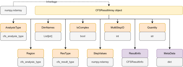
Figure 5: Structure of CFSResultArray class. Attributes are highlighted in orange, Properties in purple, and respective data types in grey.

The Quantity attribute can be chosen as any string in general. However, if the exported data will be the input of a subsequent openCFS simulation, openCFS variable names must be used for the declaration of field quantities. Thus, for the acoustic PDE, one of the following names must be chosen.

General acoustic and fluid mechanic quantities:

• acouPressure

• acouVelocity

• acouPotential

• acoutIntensity

• fluidMechVelocity

• meanFluidMechVelocity

• fluidMechPressure

• fluidMechDensity

• fluidMechVorticity

• fluidMechGradPressure

Aeroacoustic Source Terms:

• acouRhsLoad (general)

• acouRhsLoadP (Perturbed convective wave equation)

• vortexRhsLoad (Vortex sound theory)

• acouDivLighthillTensor (Lighthill’s acoustic analogy)

CFSResultInfo: Data structure containing result information for one result. Its attributes and properties are depicted in Fig. 6. The CFSResultInfo structure is redundant to the metadata contained within a CFSResultArray object!

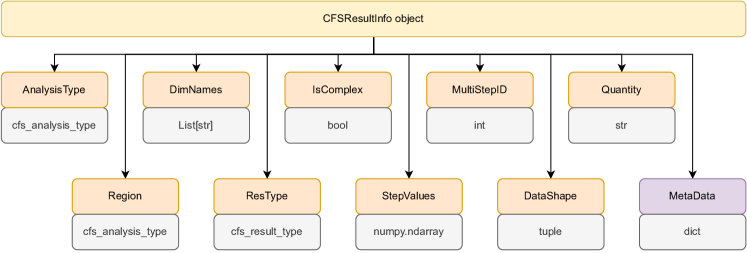
Figure 6: Structure of CFSResultInfo class. Attributes are highlighted in orange, Properties in purple, and respective data types in grey.

3 Operators for data processing (opertors)

Library of modules to perform various operations on objects in pyCFS-data data structures (see Sec. 2.3).

3.1 Interpolation operations (interpolators)

Module containing methods for interpolation operations.

3.1.1 Node2Cell

The node-to-cell interpolation operator takes nodal loads and connects them to the cell center, of the cell defined by those nodes

$$e_{\square}=\sum_{i=1}^{\mathrm{n}}v_{i}\,.$$ (1)

Thereby, $e_{\square}$ is the load located to the cell, $\mathrm{n}$ is the number of nodes of one element, and $v_{i}$ is the nodal loads. The following example shows this methodology by considering one linear triangular element:

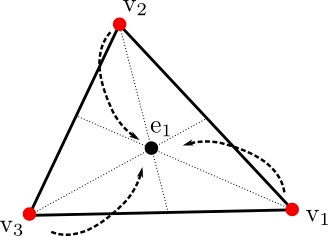
Figure 7: Cell to node interpolator.

Parameters include

• coordinates: Node coordinate array of source mesh.

• connectivity: Element connectivity array of source mesh.

3.1.2 Cell2Node

The cell-to-node interpolation operator takes element loads and divides them onto the nodes that build the cell.

$$v_{\square}=\frac{1}{\mathrm{n}}e_{i}\,.$$ (2)

The following example shows this methodology by considering one linear triangular element:

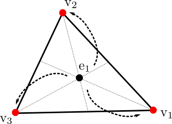
Figure 8: Node to cell interpolator.

Parameters include

• coordinates: Node coordinate array of source mesh.

• connectivity: Element connectivity array of source mesh.

3.1.3 Nearest Neighbour

The implemented nearest neighbor interpolation operator makes use of inverse distance weighting (Shepard’s method).

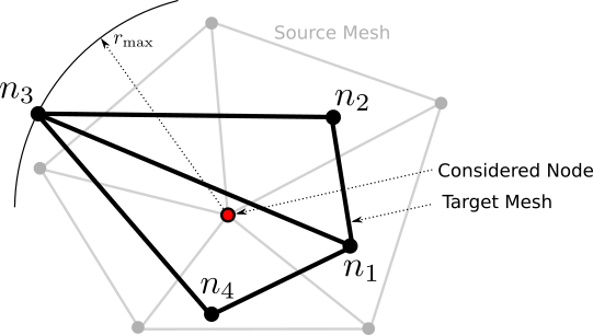
Figure 9: Nearest neighbor interpolator using ’forward’ formulation.

Based on the defined number of neighbors $n$ from the source mesh, the nearest neighbors are searched, and their distance $r$ to the considered node is computed. Based on this distances the weights $w_{i}$ are computed as

$$w_{i}=\left(\frac{R_{\mathrm{max}}-r_{i}}{R_{\mathrm{max}}r_{i}}\right)^{p}\,,$$ (3)

with $R_{\mathrm{max}}=1.01r_{\mathrm{max}}$ as being 1.01 times of the maximal distance $r_{\mathrm{max}}$, and $p$ as the interpolation exponent. Shepard stated $1\leq p\leq 3$. Increasing $p$ means that values that are further away are taken into account more. Finally, each value of each node $v_{1}$ that is taken into account is weighted to compute the new value $v_{\mathrm{n}}$ of the considered node

$$v_{\mathrm{n}}=\sum_{i=1}^{n}\frac{w_{i}v_{i}}{\sum_{i=1}^{n}w_{i}}\,.$$ (4)

Parameters include

• source_coord: Coordinate array of source positions.

• target_coord: Coordinate array of target positions.

• num_neighbors: Number of considered Nodes.

• interpolation_exp: Exponent for calculation of interpolation weight function.

• formulation: Search direction for nearest neighbor search. By default, the direction is chosen automatically based on a number of source and target points.

  • ’forward’: Nearest neighbors are searched for each point on the (coarser) target grid. This leads to a checkerboard if the target grid is finer than the source grid.

  • ’backward’: Nearest neighbors are searched for each point on the (coarser) source grid. This leads to overprediction if the source grid is finer than the target grid.

By default, the formulation is chosen automatically based on the number of source and target points.

3.1.4 Projection-based interpolation

This interpolation operator projects points of the target mesh onto the source mesh and evaluates the result based on linear FE basis functions. A comprehensive description of the algorithm can be found in [3].

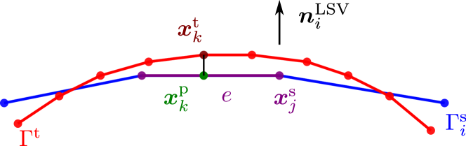
Figure 10: Projection-based interpolation. Sketch of an arbitrary source (blue) and target mesh (red) with indicated point projection from the target to the source mesh. [3]

Parameters include

• proj_direction: Direction vector used for projection. It can be specified as constant or individually for each node. By default, the node normal vector (based on averaged neighboring element normal vectors) is used.

• max_distance: Maximum projection distance. Lower values speed up interpolation matrix build and prevent projecting onto far surfaces.

• search_radius: Radius of elements considered as projection targets. It should be chosen at least to the maximum element size of the target grid.

3.2 Transformation operations (transformation)

Module containing methods for mesh/data transformation operations.

3.2.1 Fit geometry

This script fits a region to a target region using rotation and translation transformations based on minimizing the squared distance of all source nodes to the respective nearest neighbor on the target mesh. The transformation parameters are x,y,z displacement, and Euler angles.

Parameters include

• mesh_data_fit: CFSMeshData object of grid to fit

• result_data_fit: CFSResultData object of vector data to transform with mesh fit

• mesh_data_target: CFSMeshData object of target grid

• transform_param_init: Initial transformation parameters

4 Compatibility with other data formats (extras)

Library of modules to read from, convert to, and write in various formats.

4.1 Ansys Mechanical (ansys_io)

Module containing data processing utilities for reading Ansys RST files. Highlights currently include:

• Reading Ansys result files (*.rst) into CFSMeshData and CFSResultData objects.

This submodule make use of Ansys Data Processing Framework (DPF), which is not a standard requirement of pyCFS. The additional dependencies can be installed via pip using pip install pycfs[data]. This submodule make use of Ansys Data Processing Framework (DPF), which is in Beta development stage. Therefore, compatibility might break rapidly. The methods in this submodule make use of Ansys Data Processing Framework (DPF), which requires a licensed installation of the according DPF Server!

4.2 EnSight Case Gold (ensight_io)

Module containing data processing utilities for reading EnSight Case Gold files. Highlights currently include:

• Reading EnSight Case Gold files into numpy arrays (Mesh and Time series)

• Conversion to CFSMeshData and CFSResultData objects.

4.3 Polytec PSV export data (psv_io)

Module containing data processing utilities for reading universal files (UFF) exported from PSV Software. Highlights currently include:

• Reading universal files (UFF) into dict format compatible to sdypy-EMA.

• Trilaterate scanning head position from export data.

• Combine three 1D measurements into 3D data.

• Conversion to and from CFSMeshData and CFSResultData objects into sdypy-EMA compatible dict format.

4.4 NiHu Matlab export data (nihu_io)

Module containing data processing utilities for reading NiHu structures as Matlab export files. Highlights currently include:

• Conversion of NiHu mesh Matlab structure into CFSMeshData object.

5 Acknowledge

We would like to acknowledge the authors of pyCFS and openCFS.

References

- [1] E. Mušeljić and A. Wurzinger. pyCFS – Python library for automating and data handling tasks for openCFS. https://opencfs.gitlab.io/pycfs, 2024. Accessed: 2024-04-23.
- [2] S. Schoder and K. Roppert. opencfs: Open source finite element software for coupled field simulation–part acoustics. arXiv preprint arXiv:2207.04443, 2022.
- [3] A. Wurzinger, F. Kraxberger, P. Maurerlehner, B. Mayr-Mittermüller, P. Rucz, H. Sima, M. Kaltenbacher, and S. Schoder. Experimental prediction method of free-field sound emissions using the boundary element method and laser scanning vibrometry. Acoustics, 6(1):65–82, 2024.