Implantable Adaptive Cells: differentiable architecture search to improve the performance of any trained U-shaped network

Abstract

This paper introduces a novel approach to enhance the performance of pre-trained neural networks in medical image segmentation using Neural Architecture Search (NAS) methods, specifically Differentiable Architecture Search (DARTS). We present the concept of Implantable Adaptive Cell (IAC), small but powerful modules identified through Partially-Connected DARTS, designed to be injected into the skip connections of an existing and already trained U-shaped model. Our strategy allows for the seamless integration of the IAC into the pre-existing architecture, thereby enhancing its performance without necessitating a complete retraining from scratch. The empirical studies, focusing on medical image segmentation tasks, demonstrate the efficacy of this method. The integration of specialized IAC cells into various configurations of the U-Net model increases segmentation accuracy by almost 2% points on average for the validation dataset and over 3% points for the training dataset. The findings of this study not only offer a cost-effective alternative to the complete overhaul of complex models for performance upgrades but also indicate the potential applicability of our method to other architectures and problem domains.

[ref:affiliation]organization=Computer Science Institut, Maria Curie Sklodowska University, addressline=Akademicka 9 Street, city=Lublin, postcode=20-033, country=Poland

1 Introduction

The development of specialized neural network architectures remains a significant challenge in the field of deep learning. The best neural network architectures very often depend on the problem they solve and require careful consideration of various aspects of the network topology, including depth, connections between operations, kernel sizes, activation functions, and normalization methods. The complex nature of this process results in the need for significant expertise and time investment, making the design of an optimal network a formidable challenge. Therefore, the concept of Neural Architecture Search (NAS) has emerged as an automatic process for discovering suitable neural network architectures. The success of NAS in classification tasks has encouraged researchers to extend this approach to segmentation problems [1]. Many NAS algorithms have been presented that automate the process of designing neural network architectures for semantic segmentation using various methods, e.g. evolutionary algorithms, reinforcement learning, or gradient-based architecture search [2, 3, 4, 5]. The utilization of NAS has also gained traction in the field of medical data, which often comprises high-resolution images and necessitates precise pixel-level predictions [6, 7, 8, 9, 10, 11]. Notably, most of these studies emphasize gradient methods due to the characteristics of medical data and the high computational requirements of segmentation models. The gradient-based NAS method, called Differentiable Architecture Search (DARTS), initially proposed in [12] to solve classification problems, is continually being optimized in developments such as [13, 14, 15, 16]. However, techniques like NAS-Unet [7] and DiNTS [10] typically lead to the creation of entirely new architectures that require training of these networks from scratch with extensive datasets. Nevertheless, there is no research that could demonstrate whether and how the performance of existing and trained architectures can be improved by integrating small and lightweight modules. In particular, modules that are generated within a specific neural network and tailored to it. This research gap highlights the need for alternative strategies that could improve and extend the capabilities of existing neural networks without having to completely rebuild and retrain them from scratch. To address this gap, in this article we introduce a differentiable process for searching small blocks of operations within an already trained network. These blocks, due to their ability for seamless integration into the existing architecture, are referred to as Implantable Adaptive Cells (IAC). The search process (and later also the generated IACs) is located on the skip connections of the U-Net [17] type architecture commonly used for tasks related to medical image segmentation (see Fig. 1). To identify the architecture of these cells, we present an efficient search method based on PC-DARTS [14]. The input to our method is a pre-trained U-Net model and a set of training data, and its goal is to find a suitable Implantable Adaptive Cell that, once placed on the skip connections, improves the effectiveness of this network. At each stage of resolution, the same cell architecture is generated, but with different parameters (weights), which leads to multiple extraction of features at different scales in different ways, thus the coarse features provided by skip connections are processed differently depending on the resolution of the features and the level of architecture.

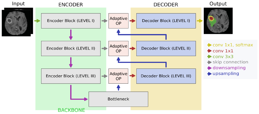
Figure 1: Diagram of the U-Net architecture, in which we search for Implantable Adaptive Cells (IAC) and then integrate them into the networks using our proposed methodology. It is worth noting that the BACKBONE is intentionally varied. In this diagram, Adaptive OP represents different operations depending on the stage: a simple concatenation operation (Stage I), an Implantable Adaptive Cell in continous form (Stage II), and an Implantable Adaptive Cell in discrete form (Stage III). The Stages are described in detail in Section 4.2.

The main contributions of our approach include:

1. Development of a method that generates an Implantable Adaptive Cell (IAC) compatible with any encoder architecture within the U-Net network.

2. Enhancement of pre-trained U-Net models through the integration of IAC into their skip connections, thereby improving their effectiveness and generalization.

3. Introduction of the concept of IAC capable of processing both low-level and high-level features within the network.

4. Introduction of an innovative application of the DARTS and PC-DARTS methods in neural network training and optimization.

5. Analysis and resolution of the discretization gap issue in differentiable search methods applied to pre-trained neural networks.

To facilitate further research and application, we have made the source code of our implementation publicly available at:
https://gitlab.com/emil-benedykciuk/u-net-darts-tensorflow.

2 Related works

In recent years, deep neural networks have emerged as a powerful tool for automating the segmentation of medical images, which is a key step in many clinical applications. However, the accurate separation of pathological changes from normal tissues in MRI images remains a challenging task, and often requires the design of specialized neural network architectures.

2.1 Medical image segmentation

The field of biomedical image analysis has been revolutionized by the seminal work of O. Ronnenberger et al., as published in their paper [17]. Their proposed U-Net neural network architecture was specifically designed for two-dimensional biomedical image segmentation. The U-Net architecture consists of an encoder-decoder structure, where the encoder is responsible for feature extraction and learning representations at increasingly higher levels, while the decoder reconstructs these features to higher resolution to obtain dense predictions. This has demonstrated high accuracy in segmentation tasks, leading to numerous modifications and improvements, such as Attention U-Net [18] and RAUnet [19] which which introduce attention mechanisms to U-Net. UNet++ [20] redesigns skip connections using dense blocks. In turn, nnU-Net [21] combines U-Net, 3D U-Net [22], and cascaded 3D U-Net [23], focusing on determining optimal configurations and hyperparameters to further advance the performance of the final architecture. This architecture achieved the best results in comparative tests of medical image segmentation (e.g. won Medical Segmentation Decathlon (MSD) Challenge [24]).

Skip connections in U-Net networks are essential for medical image segmentation, as they transfer high-resolution feature maps from the encoder to the decoder, retaining crucial spatial information. These connections enable the decoder to access various levels of abstraction from the encoder, enhancing the detail recovery in segmentation outputs. This is vital for accurately delineating small and indistinct features in medical images. However, they can also introduce errors by either over- or under-segmenting due to limitations in feature detail transfer. To overcome these issues, enhancements such as attention mechanisms, convolutional layer assemblies, and dense blocks have been developed to refine the features transmitted through skip connections, focusing on eliminating irrelevant areas and accentuating task-specific features [18, 19, 20].

2.2 Neural architecture search

Recent advancements in neural architecture search (NAS) have generated significant interest in the research community. Early NAS approaches involved using reinforcement learning (RL) [25, 26] or evolutionary algorithms (EA) [27] to discover efficient neural network architectures, which were then trained using gradient-based optimization methods. However, these methods suffer from high computational costs due to the iterative nature of architecture search and parameter optimization. To reduce these costs, more efficient NAS techniques have been developed. One-shot models have emerged as a time-saving approach, using methods like hypernetworks [28] and weight sharing [29] for architecture search. Additionally, [30] demonstrated that one-shot models could predict architecture performance effectively using just gradient descent.

A promising approach to address the challenge of the resource-intensive nature of NAS is to use gradient-based methods for searching an optimal neural network. Differentiable Architecture Search (DARTS) [12] introduced a gradient-based approach that significantly lowers computational demands by using continuous variables for architecture components, optimizing both network weights and architecture parameters. Despite its efficiency, DARTS faced issues like instability and performance collapse, as noted in [31]. Subsequent iterations like PDARTS [32] and PC-DARTS [14] aimed to improve memory efficiency and solve operational inconsistencies. Challenges such as operation co-adaptation and biases in architecture selection were addressed in further studies [13, 15, 16, 33, 34], highlighting ongoing efforts to refine NAS methodologies.

Recent studies like those by [2, 3, 4, 5] have explored NAS for natural image segmentation. Mortazi and Bagci [6] developed a method for optimizing hyperparameters in densely connected networks, while [7] experimented with different operations for constructing U-Net architectures. Challenges persist in adapting successful NAS methods from natural to medical imaging, as highlighted by [8] in 2019. Several approaches have focused on enhancing the U-Net structure or exploring alternative architectures. [9, 35] modified edge operations within the U-Net framework, while others like Auto-DeepLab [2] and FasterSeg [3] utilized advanced search spaces to design networks optimized for both cellular and spatial resolution changes. MS-NAS [36] applied principles from PC-DARTS to 2D medical images, and evolutionary algorithms were used in [37] to explore new architectures. DiNTS [10] employed a differentiable NAS approach for segmentation, achieving significant results in the 2021 Medical Segmentation Decathlon [38]. Following this, HyperSegNAS [11] outperformed DiNTS in 2022 using a novel HyperNet-based architecture called Meta-Assistant Network (MAN), which adjusts channel-wise weights based on high-level architecture and image information for improved segmentation performance.

3 Method

Based on the existing literature we posit that the incorporation of differentiable architecture search methods in the skip connections could potentially pave the way for identification of better structures, which may even more escalate the network’s capacity to learn more intricate features, all the while maintaining the preservation of spatial information. To the best of our knowledge, there have been no prior attempts to utilize NAS techniques for the purpose of generating additional modules in the skip connections that seamlessly integrates with a pre-designed, trained architecture. Specifically, this gap in the literature pertains to the application of NAS methods in the context of biomedical data for semantic segmentation purposes.

3.1 Base network topology

In our research, we use 2D U-Net architecture [17], referred to as base U-Net. We rely on the base U-Net due to its simplicity and effectiveness, as previous research has shown its superior performance compared to other architectures. Our decisions are guided by experiences with nnU-Net presented in [21], where researchers take away superfluous elements of many proposed network designs. To evaluate the generated cell architecture, we train various U-shaped architectures with modifications to the encoder. Specifically, we replace the base architecture with different backbones, such as EfficientNetB0-7 [39], ResNet [40] and others, while keeping the U-shaped structure intact. This allows us to assess the performance and compare the efficacy of our cell in different U-Net frameworks. This analysis helps us understand the influence of the cell architecture on the overall performance of the U-shape models in our specific medical image segmentation task.

3.2 Implantable Adaptive Cell architecture

We define our Implantable Adaptive Cell (IAG) as a compact directed acyclic graph (DAG) consisting of $\mathcal{N}$ nodes, where each node represents a hidden feature representation. The transformation of feature tensors between a pair of nodes is performed by edges, which correspond to the selected operations to be executed. Each edge encompasses $\mathcal{M}$ candidate operations, offering a diverse array of potential transformations (see Fig. 2). Notably, each edge and its associated operation have independent weights, called architecture parameters, discussed further in Section 3.2.2. The cell functions as a fully convolutional module, where the input for each node results from a weighted sum of operations originating from all previous nodes. It’s important to note that we are still discussing the continuous architecture representation of the cell at this stage.

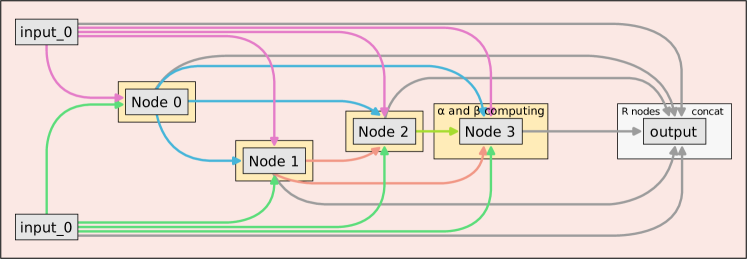
Figure 2: A simple general diagram of the Implementable Adaptation Cell, where input₀ are coarse features procured via skip connections from the encoder, and input₁ are upsampled features gleaned from the previous decoder block. The proposed method searches for connections between nodes and operations between them.

Our Implantable Adaptive Cell is strategically located within the U-Net architecture (see Fig. 1). Regardless of the level within the U-Net architecture, exactly one cell architecture is generated. Specifically, the architecture parameters are shared across all cells at every level, while cell weights are trained independently. These cell weights refer to the weights of the trainable operations on the edges of the defined graph and trainable operations that process input and output. In summary, this single cell architecture is utilized across various levels and is replicated across all skip connections in the network topology, with each cell at different levels having distinct weights and operation outcomes.

As the Adaptive Cells are placed on skip connections, they have two inputs and one output. The inputs of the cell are respectively coarse features procured via skip connections from the encoder, and features collected from the previous decoder block which are then upsampled (see Fig. 1). Due to the architecture’s high complexity and relatively expansive search space, the data entering the cell undergo a $1\times 1$ convolutional layer processing to attenuate the number of feature maps. Even at this phase, the quantity of convolutional filters for each operation within the cell is predefined. This value varies depending on the level within the U-Net architecture where the cell is positioned. The cell’s output is formed by a concatenation of the feature maps extracted from the final $\mathcal{R}$ nodes. Ultimately, to achieve a number of feature maps corresponding with the appropriate level as per the U-Net architecture, the cell output also undergoes a $1\times 1$ convolution operation, equipped with an appropriate number of filters. The above ensures that the cell will adapt to any architecture, irrespective of how many feature maps the coarse feature blocks and the upsampled data from the previous decoder block contain. The number of output feature maps matches the sum of the feature maps derived from both the skip connection and the preceding decoder block.

The continuous representation of the Implantable Adaptive Cell described above is used to identify the appropriate cell, which we obtain through discretization (see Section 3.2.3).

3.2.1 Search space

The cell search space is defined as a collection of fundamental operations wherein input and output feature maps maintain identical spatial resolution. A selection of simple operations is employed, with constraint on their quantity, to address the substantial memory resource requirements associated with U-shaped architectures. The delineation of the cell search space constitutes a pivotal component, as it specifies the assortment of prospective operations and design alternatives explored by the learning algorithm for architectural optimization.

Notwithstanding the aforementioned considerations, the operations delineated in the original DARTS [12] and PC-DARTS [14] works are selected for this study. This choice stems from the study’s primary objective, which entails examining the capability of differentiable NAS algorithms in discovering cells for pre-existing and trained architectures. Consequently, the simplicity of the operations proposed in the original work suffices for this purpose. Based on the original search space, each cell in our architecture consists of four intermediate nodes, with a total of 14 edges. Each edge is associated with 8 candidate operations, providing a range of options for information flow and feature extraction within the cell. The designated set of search space operations encompasses: zero (no connection), identity (skip connection), $3\times 3$ max pooling, $3\times 3$ average pooling, $3\times 3$ and $5\times 5$ separable convolutions, and $3\times 3$ and $5\times 5$ dilated separable convolutions.

3.2.2 Continuous relaxation and optimization

The continuous relaxation, as described in PC-DARTS, is employed to facilitate the selection of suitable operations between nodes in the defined graph - our Adaptive Cell. Therefore, we conducted a review of the baseline DARTS and PC-DARTS, and we established the notations pertinent to subsequent discussions. To introduce flexibility in the architecture search, a mixed operation (also known as a ”mixture” or ”softmax” operation) is utilized. In this case, a continuous relaxation of the search space is employed, allowing the algorithm to use gradient-based optimization for efficient architecture search. The mixed operation computes a weighted sum of all candidate operations on an edge, where the weights are learnable parameters optimized during the search process. To be more precise we denote a predefined space of operations by $\mathcal{O}$, in which each element, $\mathit{o}(\cdot)$, is a fixed operation performed on the node tensor. Within a cell, the goal is to choose one operation from $\mathcal{O}$ to connect each pair of nodes, in other words, to determine the edges of our graph. Let a single edge between two nodes be $(i,j)$, where $0\leq i<j\leq\mathcal{N}-1$, where $\mathcal{N}$ is number of nodes as mentioned at the beginning of the Section 3.2, the core idea of DARTS is to formulate the information propagated from $i$ to $j$ as a weighted sum over $|\mathcal{O}|$ operations:

$$\varphi_{o}=\frac{\exp(\alpha^{o}_{i,j})}{\Sigma_{o^{\prime}\in\mathcal{O}}\exp(\alpha^{o^{\prime}}_{i,j}))}$$ (1)

$$f_{i,j}(x_{i})=\sum_{o\in\mathcal{O}}{\varphi_{o}\cdot(x_{i})}$$ (2)

where $x_{i}$ is the output of the $i$-th node, and is an architecture parameter for weighting operation $\mathit{o}(x_{i})$. The output of a node is the sum of all input flows, i.e. $x_{j}=\Sigma_{i<j}f_{i,j}(x_{i})$, and the output of the entire cell is formed by concatenating the output of $\mathcal{R}$ last nodes $x(n-\mathcal{R}-1)-x(n-1)$. Note that the first two nodes, $x_{0}$ and $x_{1}$, are input nodes to a cell, which are fixed during architecture search. In accordance with this parameter, operations are chosen to comprise the final architecture of the Adaptive Cell, as explained in Section 3.2.3.

For better memory efficiency, PC-DARTS introduced a partial channel connection and thus extended expression (1) with additional operations. Consider the edge between nodes $i$ and $j$, this allows us to define the channel sampling mask as $S_{i,j}$ (1 assigned to selected channels, 0 to the omitted ones). The selected channels are sent into mixed computation of $|\mathcal{O}|$ operations, while the masked ones are directly copied to the output

$$f^{PC}_{i,j}(x_{i};S_{i,j})=\sum_{o\in\mathcal{O}}{(\varphi_{o}\cdot o(S_{i,j}*x_{i}))}+(1-S_{i,j})*x_{i}$$ (3)

where $S_{i,j}*x_{i}$ and $(1-S_{i,j})*x_{i}$ denote the selected and masked channels, respectively. It is noteworthy that, to regulate the quantity of selected channels for above computations (mask $S_{i,j}$), the $\mathcal{K}$ hyperparameter is introduced. This parameter enables the selection of a $1/\mathcal{K}$ fraction of channels exclusively for calculations, thereby achieving a $\mathcal{K}$-times reduction in memory consumption. The idea of masking channels and selecting only part of them to choose one operation from O (optimizing the $\alpha$ architecture parameter) is shown in Fig. 3, keeping the symbols consistent with the discussed formulas.

Unfortunately, the aforementioned modification introduces a degree of instability in the edge selection process between nodes, which is large anyway. Consequently, the authors of PC-DARTS opt to implement edge normalization using an additional architecture parameter $\beta$ to dampen undesirable oscillations in the resulting network architecture. We recommend reviewing the visual representation of this process as shown in Fig. 4. This figure uses symbols consistent with previously described patterns. Specifically, Fig. 4 illustrates the incorporation of the PC-DARTS process, emphasizing the Partial Channel Block along with its corresponding colors, as seen in Fig. 3. This visualization is focused on demonstrating the integration of the PC-DARTS process in the optimization of the $\beta$-cell architecture parameters.

For edge $(i,j)$, this normalization yields the subsequent expression:

$$\Psi_{i,j}=\frac{\exp(\beta_{i,j})}{\Sigma_{i^{\prime}<j}\exp(\beta_{i^{\prime},j})}$$ (4)

$$x^{PC}_{j}=\sum_{i<j}{(\Psi_{i,j}\cdot f_{i,j}^{PC}(x_{i};S_{i,j}))}$$ (5)

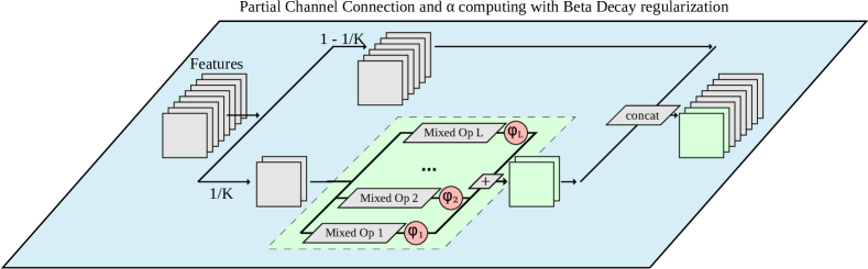
Figure 3: A visual representation of a cell architecture search by continuously relaxing the search space by placing a mixture of candidate operations on each edge. In this search step, the $\alpha$ architectural parameter is determined which is for a particular edge $\alpha^{o}_{i,j}$ tries only a subset of 1/K channels and connects them to the next step so that the memory consumption is reduced by K times. In this step $\alpha$ is used to calculate $\varphi_{o}$.

By employing a differentiable approach, we enable the search for adaptive cell architectures to be conducted through bi-level optimization, with the aim of solving the following objective function:

$$\underset{\alpha,\beta}{\text{min}}\phantom{x}{\mathcal{L}_{val}(\omega^{*}(\alpha,\beta),\alpha,\beta)}$$ (6)

$$\text{s.t.}\phantom{x}\omega^{*}(\alpha,\beta)=argmin_{\omega}{\mathcal{L}_{train}(\omega,\alpha,\beta)}$$ (7)

In practice, the adaptive cell architecture parameters $\alpha$ and $\beta$, as well as the cell weights $\omega$, are updated iteratively using gradient descent on both the validation and training datasets. The cell weights $\omega^{*}$ are approximated by taking a one-step forward on current $\omega$ during the optimization process DARTS. Referring to above, during the search procedure, the introduced relaxation method enables the simultaneous learning of the adaptive cell architecture parameters and weights. Notably, the weights of the U-Net network $\omega^{\prime}$ are frozen during the search stage, ensuring compatibility between the identified cell architecture and the feature maps generated by the existing network. This approach facilitates the discovery of a cell architecture that seamlessly integrates with the established network while leveraging its learned representations effectively. In our methodology, we employ the simpler optimization strategy of one-step forward for updating the weights $\omega$ of the cells. This choice is motivated by considerations of practicality and computational efficiency. Furthermore, we draw inspiration from the successful utilization of this strategy in PC-DARTS, which demonstrates its efficacy in addressing the limitations associated with this approach through regularization effects.

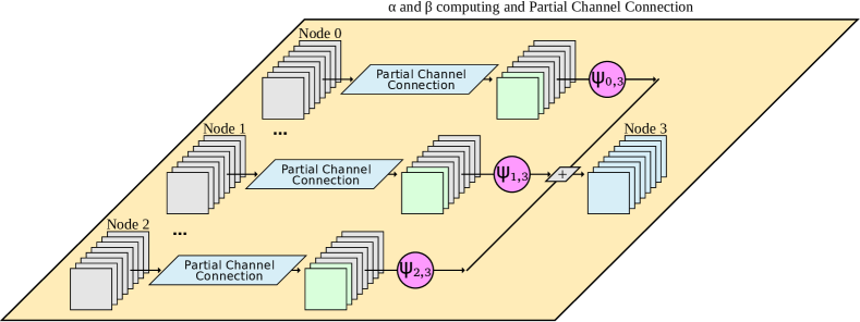
Figure 4: A visual representation of the process of searching for node connections that minimize the uncertainty provoked by sampling (refer to Fig. 3).

To mitigate the risk of overfitting the architecture parameters to the training data, we partition the training set into two distinct subsets (more detail in Section 4.1): train_search_dt and val_search_dt. Within each iteration, we first fix the weights of the cells ($\omega$) and update the architecture parameters ($\alpha$ and $\beta$) using the val_search_dt subset. Subsequently, we fix the architecture parameters $\alpha$ and $\beta$, and update the weights of the cells ($\omega$) using the train_search_dt subset. It is important to note that although all cells share the same architecture parameters ($\alpha$ and $\beta$), they possess independent weights ($\omega$). To evaluate the performance of our approach, we employ the Dice loss as our chosen loss function.

3.2.3 Discretization

There exist two distinct sets of architectural parameters necessitating discretization after the conclusion of the optimization process. The first parameter set dictates the selection of operations $\mathit{o}$ on a given edge ($\alpha$), with the second governing the choice of edges between nodes ($\beta$). During the $\alpha$-discretization phase, the operation with the highest parameter value between input and output nodes is selected, typically involving a single edge between two nodes $(i,j)$. Nevertheless, the additional operations can still have a significant influence on the feature map values at the exit node $j$. The immediate dismissal of non-zero operations may culminate in a discretization gap. An identical problem is likely to occur during the $\beta$-discretization stage, which involves the selection of input edges entering node $j$. Essentially, each node within our cell architecture possesses two input edges. This discretization gap is a consequence of the continuous model sought-after being inherently non-binary. Consequently, certain operations or edges with small, yet non-zero probabilities, are rejected during the discretization phase. Disturbingly, this impact elevates in correspondence with the complexity of the cells. Nonetheless, it is evident that this particular issue has not been addressed in the current study, primarily due to its distinct research parameters. However, we deem it necessary and important to acknowledge this knowledge gap for a comprehensive understanding of the subject matter.

4 Results

In an effort to promote transparency and reproducibility of our research within the scientific community, we have prioritized the deterministic implementation of operations and the learning procedures for our neural networks. As such, we have made our source code publicly accessible via the following URL: https://gitlab.com/emil-benedykciuk/u-net-darts-tensorflow. We encourage fellow researchers to utilize this resource in the spirit of collaborative scientific advancement.

4.1 Dataset

The International Brain Tumor Segmentation Challenge (BraTS) presents a platform for evaluating state-of-the-art methods revolving around brain tumor segmentation. The challenge offers a valuable asset in the form of a 3D MRI dataset, complete with ground truth tumor segmentation labels furnished by physicians [41, 42, 43]. The 2023 iteration of the challenge retains its focus on the generation of a shared benchmarking environment. However, the dataset sees substantial expansion, approximating 4,500 cases, to cater to additional factors like different populations (i.e. sub-Saharan African patients), diverse tumors (i.e. meningioma), new clinical concerns (i.e. missing data), and technical considerations (i.e. augmentations). The fundamental objective of the BraTS 2023 [43] is the identification of top-tier algorithms capable of addressing many problems, including the one identified as Task 1 in BraTS, which is the same adult glioblastoma population featured in the RSNA-ANSR-MICCAI BraTS challenge, on which we concentrated our research.

Significantly, all data incorporated are clinically-acquired, routine, multi-site multiparametric magnetic resonance imaging (mpMRI) scans of brain tumor patients. The BraTS training and validation data available for download and methodological development by participating teams comprise a total of 5,880 MRI scans from 1,470 brain diffuse glioma patients, and stand identical to the data curated for the RSNA-ASNR-MICCAI BraTS Challenge. The data, accessible as NIfTI files (.nii.gz), includes a) native (T1) and b) post-contrast T1-weighted (T1Gd), c) T2-weighted (T2), and d) T2 Fluid Attenuated Inversion Recovery (T2-FLAIR) volumes, and was procured through various clinical protocols and various scanners from multiple data contributing institutions. Each study consists of four rigidly aligned 3D MRI modalities, resampled to a 1x1x1 mm isotropic resolution and skull-stripped, with the input image size being 240x240x155. The provided annotations differentiate three tumor subregions: the GD-enhancing tumor (ET), the peritumoral edema/invaded tissue (ED), and the necrotic and non-enhancing tumor core (NCR).

We trained our networks on input data represented by two distinct MRI modalities: T1Gd and T2-FLAIR, which were merged to form a two-channel image with a resolution of $240\times 240$ and a suitably labeled output mask. This input and output are cropped to a resolution of $128\times 128$ in order to minimize the number of background voxels. The mask constitutes a binary map for all four classes prepared in the context of BraTS 2023 collection, ET – label 3, ED – label 2, NCR – label 1, and BG – label 0 (background). To ensure a fair evaluation of our modified U-Net, we refrained from augmenting datasets and any randomness related with the data preprocessing. Notably, the training dataset was partitioned into several sections as documented in Fig. 5. This consisted of a training set (train_dt), comprising 80% of the entire dataset, and a validation set (val_dt), containing the remaining data, where various U-Net networks were trained and verified. In addition, equal subsets (train_search_dt and val_search_dt) were partitioned from train_dt, serving to facilitate the search for an optimal cell architecture (refer to section 4.2). This gives us datasets with the following number of dual-channel images with a resolution of $128\times 128$: train_dt - 64896, val_dt - 16256, train_search_dt - 32384, val_search_dt - 32384 (the differences in sample sizes are due to adjusting their numbers to the size of the batches) Finally, following the addition of the generated adaptive cell to any pretrained U-Net, the network was again trained on train_dt and verified on val_dt.

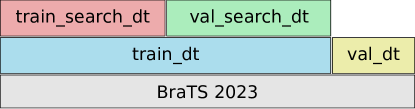
Figure 5: This figure presents an overview of the datasets that have been meticulously developed. The construction of these diverse training and validation sets employed a part of the data from the BraTS 2023 set that covered Task 1 – the segmentation of the adult glioblastoma. The base U-net architectures were trained utilizing train_dt and val_dt sets, effectively serving as reference points in our studies. These datasets were also used in the training of the networks to which the IAC cell had been integrated. Two equally numbered sets, train_search_dt and val_search_dt, exclusively derived from the train_dt set, were used in uncovering the adaptive cell’s architecture.

4.2 Adaptive Cell search conditions and implementation details

In this section, we present the details of our experiments. These were designed to evaluate the efficiency of the proposed Adaptive Cells. We also examine their scalability and their potential applicability to multiple U-shaped networks. The entire procedure was conducted in 3 main Stages: (I) preparation of the base networks, (II) searching for IAC, (III) training the IAC within the network.

4.2.1 Stage I - Preparing benchmark U-Nets

Our supernet $\boldsymbol{\mathcal{S}}$ is engineered upon the foundational structure of the conventional U-Net, as illustrated in Fig. 1. The network’s two-channel input images feature a resolution of $128\times 128$, while the four-channel output warrants an equivalent $128\times 128$ resolution, where each channel is representative of one of the 4 classes defined in Section 4.1. This cell-free network, which involves standard concatenation in skip connections, undergoes training by 200 epochs on the train_dt set. Its effectiveness concerning the Dice metric on the validation set val_dt is evaluated during every epoch. These training outcomes, presented in Table 1, serve as a standard point of reference for our proposed solution. All reference networks were trained using Adam optimizer with a constant learning rate of $0.001$. The loss function is represented by the Dice metric. A consistent batch size of $128$ was maintained across all networks featuring diverse backbones (referring specifically to the encoder component of U-Net, as represented in Fig. 1. This initial phase of our research, termed Stage I, does not necessitate employment of our proposed method. However, in the context of this study, it serves solely as a benchmark to test the functionality of the generated cells under a variety of conditions, that is, U-shaped architectures boasting different feature extraction encoders.

Table 1: Reference results for different U-Net-s. The table illustrates the performance range of U-Net with diverse backbone structures (as represented in Fig. 1), employing the Dice metric for evaluation. The table highlights epochs wherein the model obtained the optimum result for the val_dt. Furthermore, the table shows the time of a single epoch, which is to serve as a reference for assessing the duration of the search process (Stage II) and the training for the network with the Adaptation Cell (Stage III). The column labeled TRAIN DICE displays the outcomes for the training data set denoted as train_dt, whereas the VAL DICE column illustrates the results for the validation data set, termed val_dt. Moreover, the column entitled EPOCH specifies the epoch at which the neural network yields the optimum result. Subsequently, the number of trainable network parameters is given in the TRAINABLE PARAMS column.

BACKBONE	TRAIN DICE	VAL DICE	EPOCH	TRAINABLE PARAMS
Base	0.8106	0.6073	168	487236
VGG16	0.8577	0.7971	197	8195434
ResNet50	0.8534	0.5919	167	1982506
EfficientNetB0	0.7951	0.7101	27	396364
EfficientNetB3	0.8495	0.7528	85	567768
EfficientNetB5	0.8809	0.7782	193	957066
EfficientNetB7	0.8702	0.7852	139	1591014

4.2.2 Stage II - Searching Adaptive Cell for appropriate U-Net architecture

The succeeding phase of our research, positioned as the focal point of this study and the described methodology, is dedicated to developing an Implantable Adaptive Cell. The objective of this identified cell is to strengthen a U-network-like structure designed to solve the particular problem (in the current scenario, brain tumor segmentation). Details regarding the methodology for the cell architecture search have been outlined in Section 3. Additionally, implementation specifics, correlating to the figures included in our paper, are illustrated in Algorithm 1 and Algorithm 2.

Algorithm 1 U-Net adaptive cell search (Stage II).

1:Adaptive cell architecture parameters $\boldsymbol{\alpha}$ and $\boldsymbol{\beta}$; Adaptive cell weights $\boldsymbol{\omega}$; Trained vanilla U-Net weights $\boldsymbol{\omega}^{\prime}$, Number of search epochs $\boldsymbol{\mathcal{E}}$; Training dataset train_search_dt; Validation dataset val_search_dt; Regularization coefficient adjustment schema $\boldsymbol{\lambda_{e},e\in\{1,2,...,\mathcal{E}\}}$; Number of steps in one epoch $\boldsymbol{\mathcal{Z}=|train\_search\_dt|=|val\_search\_dt|}$; Loss function $\boldsymbol{\mathcal{L}}$;

2:

3:Construct a supernet $\boldsymbol{\mathcal{S}}$ (see Fig. 1) and load U-Net weights $\boldsymbol{\omega}^{\prime}$

4:Initialize architecture parameters $\boldsymbol{\alpha}$, $\boldsymbol{\beta}$ with ones and random initialize cells’ weights $\boldsymbol{\omega}$

5:Freeze all weights except $\boldsymbol{\alpha}$, $\boldsymbol{\beta}$, $\boldsymbol{\omega}$ parameters

6:

7:for each $e\in[1,\mathcal{E}]$ do

8:     for each $z\in[1,\mathcal{Z}]$ do

9:          Compute loss value $\boldsymbol{\mathcal{L}_{val\_search\_dt}}$ on the val_search_dt based on step forward through the supernet $\mathcal{S}$ (see Algorithm 2 for more cell’s step forward details)

10:         Update $\boldsymbol{\alpha}$ and $\boldsymbol{\beta}$ by descending $\boldsymbol{\nabla_{\alpha,\beta}\mathcal{L}_{val\_search\_dt}(\alpha,\beta,\omega)}$

11:          Compute loss value $\boldsymbol{\mathcal{L}_{train\_search\_dt}}$ on the train_search_dt based on the updated supernet $\mathcal{S}$ architecture

12:         Update $\boldsymbol{\omega}$ by descending $\boldsymbol{\nabla_{\omega}\mathcal{L}_{train\_search\_dt}(\alpha,\beta,\omega)}$      

13:Derive the final adaptive cell architecture based on the learned $\boldsymbol{\alpha}$, $\boldsymbol{\beta}$

This process, denoted as Stage II, revolves around the creation of a supernet $\mathcal{S}$ in compliance with Fig. 1 (including a continuous representation of cells). Subsequently, the weights $\omega^{\prime}$ of the trained standard U-net are loaded, and the $\alpha$ and $\beta$ architecture parameters are initialized to ones, while the cells’ weights $\omega$ are randomly initialized. The subsequent step involves freezing supernet weights except $\alpha$, $\beta$ and $\omega$, enabling their fitting with the pre-existing trained network. In other words, we only freeze $\omega^{\prime}$. To mitigate instability during the search process and high variability in its performance, we incorporate a ’warm-up’ stage in Stage II. The ’warm-up’ stage endures for 15 epochs and is predicated upon overtraining weights $\omega$ in cells, or in essence, overtraining all mixed operations featuring weights within cells. It is essential to reiterate that each cell possesses its independent weights (the part of the set of weights $\omega$), with the exception of shared $\alpha$ and $\beta$ architecture parameters. Following the ’warm-up’, the actual architectural search process ensues, detailed in Section 3 and Algorithms 1 and 2. During each epoch, our algorithm comprehensively traverses the train_search_dt and val_search_dt datasets. For each batch within the val_search_dt set, the value of the $\boldsymbol{\mathcal{L}_{val\_search\_dt}}$ loss function is computed. Correspondingly, the architectural parameters undergo an update based on this resultant value, replicating the procedure delineated in Algorithm 2. Subsequent to this, updated parameters $\alpha$ and $\beta$ (signifying the revised architecture of the $\mathcal{S}$ supernet) pass evaluation to derive the value of $\boldsymbol{\mathcal{L}_{train\_search\_dt}}$ for the batch of the train_search_dt set. The cell weights $\omega$ are then updated in accordance with this calculated value. Processing of the batches is repeated until the both val_search_dt and train_search_dt datasets have been fully examined for a specified number of epochs. Referring to the ablation studies from PC-DARTS, the parameter $\mathcal{K}$, which defines channel partitioning, was set to 4. For weights $\omega$ optimization we used SGD optimizer with the following hyperparameters: learning rate $0.01$, momentum $0.0$, no weight decay, while $\alpha$ and $\beta$ optimization used an Adam optimizer with a starting learning rate of $0.001$. A cosine power annealing scheduling was used to denote learning rate changes, as described in [44]. The loss function employed was Dice as stipulated by the task and Stage I. Batch size was set at 96, and the search extended 500 epochs. The diminished batch size during the adaptive cell search, which consequently prolongs 1 epoch, is intentional given that cells consume additional GPU memory. To ensure a fair appraisal of search duration, all research was performed on a consistent platform while ensuring VRAM usage across our research stages (Stage I, II, III) didn’t exceed a certain threshold.

Algorithm 2 U-Net Adaptive Cell Search - cell’s step forward.

1:Adaptive cell architecture parameters $\boldsymbol{\alpha}$ and $\boldsymbol{\beta}(\varphi,\Psi)$; Output node $\boldsymbol{j}$, its features $\boldsymbol{x}_{j}$, and features of all nodes with index smaller than $\boldsymbol{j(x_{i}\text{ where }i<j)}$; Sampling mask $\boldsymbol{S}$;

2:

3: Compute $\boldsymbol{x}_{j}$:

4: $x_{j}=0$

5: for each $i\in[0,j)$ do

6: $x_{j}+=$$\Psi_{i,j}$ * Compute edge $i$, $j$ features for $x_{i}$ input

7: Return $x_{j}$

8:

9: Compute edge $i$, $j$ features for $x_{i}$ input:

10: Multiply features $x_{i}$ by sampling mask $\mathcal{S}_{i,j}$: $\eta$

11: H = 0

12: for each $o\in\mathcal{O}$ do:

13: $H+=$$\varphi_{i,j}$$*o(\eta)$

14: Multiply features $x_{i}$ by sampling mask $(1-\mathcal{S}_{i,j}):\eta$

15: Return concat($H$, $\eta$)

It is significant to acknowledge that the designated 500 epochs for the adaptive cell search phase do not represent a compulsory requirement. As inferred from the test results, a cell generated even at the 100-epoch stage exhibits valuable capabilities for some U-Net architectures, more details on this subject in Section 4.4.1. The epoch from which the cell was selected depended on the backbone of the model, and the selection was defined based on ablation studies. Although it can be defined arbitrarily, e.g. for cells obtained in the 100th, 200th or 500th epoch. However, due to the low stability of the search process (which we discuss in more detail in the following sections), it would be best to check several generated genotypes at Stage II.

4.2.3 Stage III - Train U-Net with generated Adaptive Cell

In the last stage, after identifying the continuous representation of the Implantable Adaptive Cell, we convert it to its discrete form according to Section 3.2.3. Once the cell with the desired architecture has been identified, the next step involves integrating this cell into the network’s skip-connections and retraining the cells’ parameters within that U-net architecture. For the research, we use U-Nets with different backbone networks in the encoder (trained in Stage I of our research) and apply an adaptive cell at each resolution level in all skip connections. After inserting the appropriate discrete cell architecture $\boldsymbol{\mathcal{G}}$, known as cell genotype, into the skip connections, we randomly initialize the cell weights $\omega$ and then load the weights $\omega^{\prime}$ for the appropriate U-Net. We freeze the weights $\omega^{\prime}$ and move on to the next step, which is training the adaptive cells’ weights within the network for 200 epochs. In this Stage, all hyper-parameters are the same as listed in Stage I. The details of this step are presented in Algorithm 3 and we call it Stage III. It should be added that Stage III should be performed because during the search stage, we only perform one optimization step of the cell weights $\omega$ at each algorithm’s step (see Algorithm 1). Fig 6 presents examples of the discrete form of cell genotypes generated by the algorithm at various stages of the search within the skip connections of selected U-Nets.

Algorithm 3 Any U-Net with generated Adaptive Cell.

1:Trained U-Net weights $\boldsymbol{\omega^{\prime}}$, Number of search epochs $\boldsymbol{\mathcal{E}}$; Training dataset train_dt; Validation dataset val_dt; Generated adaptive cell genotype $\boldsymbol{\mathcal{G}}$;

2:

3:Construct a supernet $\mathcal{S}$ (see Fig. 1) based on generated cell genotype $\mathcal{G}$

4:Load specific U-Net weights $\omega^{\prime}$ and freeze them

5:Random initialize cells’ weights $\omega$

6:for each $e\in[1,\mathcal{E}]$ do:

7:     Supernet $\mathcal{S}$ training steps on train_dt

8:     Supernet $\mathcal{S}$ evaluation steps on val_dt

9:Derive the final trained U-Net model with a specific adaptive cell

4.3 Dice Coefficient Results of Adaptive Cells

This section elucidates the results of our study where the discovery and training of an adaptive cell for each distinct U-Net network was executed individually. The entire research presented in this section undertaking aligns consistently with the protocols delineated in preceding chapters. Consequently, the entire protocol, as detailed in section 4.2, was enacted for each backbone previously mentioned in Table 1.

The outcomes for the cell, created during the Stage II and the discretization process, are documented in Table 2. These results corroborate the fact that a proficient search process can uncover a structure of operations embedded within skip connections, thereby enhancing the network’s performance. In this chapter, it is worth presenting a comparison of our results with simply fine-tuned base networks for an additional 200 epochs. We chose 200 epochs because in Stage III, we also train for an additional 200 epochs, but it is important to note that we do this only for the cell weights, which is slightly faster. All these results are presented in the mentioned table.

Table 2: The Stage III results for different backbone U-Net with selected the best cell’s architectures from Stage II. The table compares the results for selected cells from Stage II for each of the investigated architectures shown in Table 1 and their additional training. The STAGE I column shows the reference results, while the STAGE III column shows the results of these architectures with the introduced cells. Additionally, in the EXTRA EPOCH column, the results for architectures from Stage I that were simply fine-tuned for an additional 200 epochs are presented. The GENOTYPE EPOCH column indicates the epoch number from Stage II from which the cell genotype selected for Stage III originates. In the table, green highlights indicate where our method performed better than the reference U-Nets, while red indicates where it did not. Additionally, the best results from all three main columns are bolded.

BACKBONE	STAGE I		EXTRA EPOCH		STAGE III
	TRAIN	VAL	TRAIN	VAL	TRAIN	VAL	GEONTYPE EPOCH
Base	0.810	0.607	0.842	0.644	0.848	0.689	200
VGG16	0.857	0.797	0.881	0.793	0.882	0.812	100
ResNet50	0.853	0.591	0.880	0.577	0.880	0.597	100
EfficientNetB0	0.795	0.710	0.859	0.715	0.858	0.732	300
EfficientNetB3	0.849	0.752	0.876	0.732	0.877	0.760	267
EfficientNetB5	0.880	0.778	0.893	0.779	0.891	0.790	500
EfficientNetB7	0.870	0.785	0.895	0.767	0.898	0.773	400

Table 2 shows that our solution provides satisfactory results on every plane for both training and validation data. The exception is the U-Net network where EfficientNetB7 was introduced to the backbone, and our solution performed slightly worse on the validation set. The above suggests that introducing appropriate operations in skip connections improves the effectiveness of the network. Importantly, this improvement is not simply a result of overfitting, as the performance on the validation set also improves. Consequently, our proposed method demonstrates an enhanced capability for generalization. This is further confirmed by comparing our solution to simply fine-tuning the reference network.

Nevertheless, it should be noted that these results could potentially be even better given the inherent challenges of the differentiable neural network architecture search method. These challenges include the discretization gap and the instability of the search process, which are discussed in more detail in Section 4.4. We believe it is important to mention this because it highlights the wide range of opportunities for improving this solution. Despite these limitations, it is evident that even with these drawbacks, the solution still performs satisfactorily.

4.4 Ablation study - Adaptive Cell Search Analysis

In the following chapter, we will present the results of our ablation studies. In Chapter 4.4.1, we will address aspects of the proposed method’s time efficiency and provide a comprehensive analysis of different genotypes for each of the reference networks. In the subsequent Section 4.4.2, we will analyze the training curve of the introduced cells and discuss the potential issue of overfitting networks with the Adaptive Cells.

4.4.1 The influence of different cell genotypes

During the search process, a specific lineage of Adaptive Cells is generated, which is based both on the architecture in which the search process is located and on the initial weights assigned to cell operations. The effectiveness of the final architecture is influenced by different variations of the adaptive cells, emphasizing the importance of selecting appropriate operations in skip connections to achieve noticeable improvements in neural network performance. The results for the different cell genotypes obtained at various stages of the search process are presented in Tables 3,4. Each genotype was incorporated into the network and trained using the workflow described in Stage III. It is noteworthy that even slight modifications to the adaptive cell can lead to different outcomes, even though given the same initialization of cells’ operations weights. In Fig. 6, we present examples of genotypes generated in the search process for selected supernetworks $\mathcal{S}$. Detailed diagrams of the genotypes of all cells within the search process for each U-Net (with various backbones) are available on the project’s website https://gitlab.com/emil-benedykciuk/u-net-darts-tensorflow.

Table 3: Results of different adaptive cell genotypes. The table displays the Dice coefficient values for U-Nets with various backbones and adaptive cell genotypes, obtained at different epochs (EP) during Stage II and processed in Stage III. The TRN columns present the results for the train_dt dataset, while the VAL columns show the results for the val_dt dataset for each selected genotype. Values that surpass those of the Stage I reference data are highlighted in green, whereas those that are inferior are marked in red.

BACKBONE	EP 50		EP 100		EP 200		EP 300		EP 400		EP 500
	TRN	VAL	TRN	VAL	TRN	VAL	TRN	VAL	TRN	VAL	TRN	VAL
Base	0.841	0.666	0.842	0.675	0.848	0.689	0.848	0.662	0.848	0.662	0.848	0.662
VGG16	0.885	0.811	0.882	0.812	0.882	0.810	0.878	0.804	0.887	0.809	0.885	0.808
ResNet50	0.876	0.578	0.880	0.597	0.875	0.570	0.876	0.573	0.879	0.558	0.870	0.572
EfficientNetB0	0.859	0.713	0.856	0.706	0.850	0.701	0.858	0.732	0.857	0.701	0.856	0.686
EfficientNetB3	0.874	0.733	0.877	0.760	0.879	0.734	0.872	0.740	0.874	0.733	0.874	0.733
EfficientNetB5	0.891	0.766	0.892	0.768	0.897	0.782	0.893	0.771	0.889	0.775	0.891	0.790
EfficientNetB7	0.893	0.763	0.887	0.756	0.897	0.769	0.894	0.751	0.898	0.773	0.895	0.765

Table 4: Results of adaptive cell genotypes for manually selected epochs from Stage II and processed in Stage III. The columns (1) BEST SEARCH TRAIN, (2) BEST SEARCH VAL, and (3) BEST SEARCH TRAIN+VAL showcase the outcomes for genotypes manually chosen based on the search process results. These genotypes represent adaptive cells with the lowest loss function values for (1) train_search_dt, (2) val_search_dt, and (3) both sets combined. The corresponding epoch numbers when each cell was generated are also included in the results in columns named EPOCH. Values that surpass those of the Stage I reference data are highlighted in green, while those that are inferior are marked in red.

BACKBONE	Best search TRAIN			Best search VAL			Best search TRAIN-VAL
	EPOCH	TRAIN	VAL	EPOCH	TRAIN	VAL	EPOCH	TRAIN	VAL
Base	499	0.848	0.662	462	0.848	0.662	462	0.848	0.662
VGG16	217	0.878	0.807	458	0.885	0.808	176	0.884	0.808
ResNet50	500	0.870	0.572	89	0.880	0.597	467	0.879	0.558
EfficientNetB0	500	0.856	0.686	195	0.850	0.701	459	0.855	0.673
EfficientNetB3	500	0.874	0.733	267	0.876	0.722	267	0.876	0.722
EfficientNetB5	500	0.891	0.790	343	0.891	0.779	439	0.890	0.772
EfficientNetB7	500	0.895	0.765	286	0.894	0.751	473	0.898	0.773

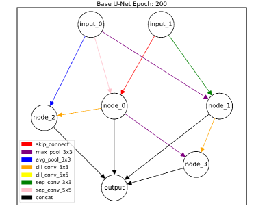
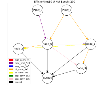
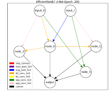
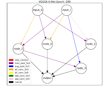
Figure 6: Example diagrams of discretized cell architectures for epoch 200 for selected supernets.

The analysis of the results presented in Tables 3, 4 indicates potential instability in the search process, i.e. Stage II. Notably, part of the networks demonstrate rapid evolution of cell genotypes, thereby impacting the outcomes in Stage III. Moreover, there are instances where the inclusion of the cell leads to improved results for the training set, but not for the validation set, implying potential over-adaptation of the network to the specific task. This effect becomes more prominent as the network complexity increases, as additionally noted in the findings presented in Section 4.4.2 regarding quicker overtraining of such networks with the adaptive cells. Here, complexity refers to the selection of operations (not only simple convolutionals blocks as Base U-Net) or the appropriate scaling of the number of parameters in relation to all planes: depth, width, resolution. Therefore, it is recommended to incorporate additional regularization methods into the search process. One possible approach is data augmentation, while another option, proposed by the authors of [45], involves regularization of the architecture parameters rather than the cell’s operations weights. It should be mentioned that our process does not employ data augmentation in order to avoid introducing additional randomness and to ensure a fair assessment of the capabilities of the method. However, it is acknowledged that data augmentation itself could significantly and positively influence the obtained results. Another recurrent issue is the instability of the search process, which arises from the nature of the method employed, specifically one-shot learning and the use of a simplified optimization approach instead of bi-level optimization.

In conclusion, the determination of an appropriate number of epochs for the search process across all networks remains a challenge, likely due to the diverse range of architectures involved. Even selecting genotypes that achieved the best results in terms of training or validation loss, or their sum, does not provide meaningful information to guide the termination of the search process or the identification of the most effective cell genotype. This limitation arises from the incomplete optimization of cell operation weights, preventing a comprehensive assessment of the suitability of adaptive cell architectures. Nonetheless, this incomplete optimization contributes to a significant reduction in the duration of the search process, a feature observed in numerous studies employing various forms of DARTS.

Tables 3, 4 effectively demonstrate that the highest performing genotype after Stage III may not necessarily be the one with the best result during the search process (Stage II). Consequently, we opted to select genotypes from different search process stages for each network with different backbones. It is also worth emphasizing that the increasing complexity of the architecture leads to intensified challenges in identifying cells that improve the generalization capabilities of the network. Furthermore, as previously mentioned, there is an increased risk of obtaining a cell that is overfit to the training data. In contrast, simpler architectures such as Base U-Net or those employing VGG16 as the backbone displayed greater ease in finding effective cells, with a greater variety of genotypes improving their effectiveness. Possibly, this is due to the over-parameterization of the backbone (large model capacity), which allows the network to remember more features and provides a chance for better generalization, and thus many opportunities for various features processing in the skip connections.

Table 5: Time efficiency of the stages. The table shows the epoch times in minutes of all three stages of the process we presented in Section 4. The STAGE III column shows only time results for cells whose results are presented in Table 2. The following measurements were performed on a computer with the following parameters: NVIDIA GeForce RTX 3090 TI, Intel Core i9-9900K, 32GB RAM, Corsair MP600 disk.

BACKBONE	EPOCH TIME [min]
	STAGE I	STAGE II	STAGE III
Base	3.682	6.340	3.752
VGG16	5.330	9.360	5.472
ResNet50	2.880	2.698	3.378
EfficientNetB0	3.502	2.748	2.822
EfficientNetB3	3.916	3.272	3.126
EfficientNetB5	5.500	4.288	5.233
EfficientNetB7	9.560	5.850	8.360

Finally, as we indicated earlier, we explain the temporal differences between epochs. It is pertinent to recall that the training phase of the reference network lasted for 200 epochs, the search phase extended over 500 epochs, and the phase for tuning the adaptation cell took 200 epochs. Table 5 shows the epoch duration in minutes for networks and genotypes of adaptive cells, as mentioned in Table 2. Notably, the epoch duration in Stage III depends on the selected architecture of the adaptive cell. Additionally, the time efficiency of the second and third stage increases as the complexity of the neural networks increases. However, it is clearly visible that for simpler architectures with a greater quantity of parameters, time efficiency is slightly lower. Nevertheless, as demonstrated previously, our approach enables the identification of an increased repertoire of adaptive cell architectures that enhance the overall performance of the network. In summary, the data presented in Table 5 indicate that the procedure is time-efficient, maintaining consistent GPU memory utilization across each network within the given backbone and throughout each stage of the process. It is important to highlight that this research was performed on a computing unit, not a supercomputing server, which implies that the described process is replicable by the majority of researchers utilizing standard home computing systems. Furthermore, it is feasible to complete the adaptive cell search for any given architecture, inclusive of its subsequent training, within a matter of hours.

4.4.2 Details of network with adaptive cells training

The graphs presented in Fig. 7 indicate that, depending on the backbone architecture, the learning curve will be similar across all adaptation cells associated with a given network. This observation aligns with the design of the Stage III, because during this stage, the network retains a consistent structure with pre-trained weights. Therefore, it is difficult to modify network capabilities using only a few operations in skip connections. It’s important to emphasize that right now, our process is focused on precisely adjusting the weights of the cells.

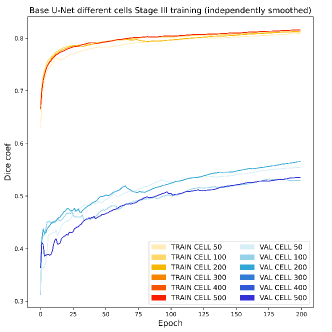
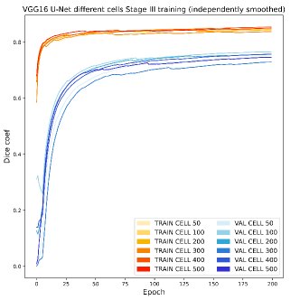
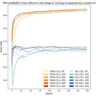
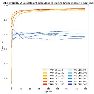
Figure 7: Example learning curve graphs for 4 selected architectures with discretized cells obtained during training in Stage III. For each architecture, 6 cell genotypes were selected from epochs in Stage II. In each graph, curves have been drawn for the train_dt (TRAIN CELL, in red–yellow color) and val_dt (VAL CELL, in bluish color) datasets.

Despite these constraints, previous results have indicated that it is feasible to engineer adaptation cells with tailored architectures and weights that enhance network performance and generalization capabilities. This is particularly important for less complex networks. Despite having a larger parameter space, these networks offer the opportunity to discover a wider range of compatible cells. This increases the network’s efficiency, a feature closely related to the network’s ability to generalize. The learning curves support this finding, illustrating that for such networks, the integration of an adaptation cell can indeed improve generalization capabilities, confirming the hypotheses presented in Section 3. Adding carefully chosen operations to the skip connections helps keep the spatial information as it moves through the network’s encoder-decoder pathway. This makes it easier for the network to learn more complex features and improves the accuracy of segmentation.

In contrast, for more complex networks that are optimized with regard to operations diversity and parameter count, adaptation cells have a lesser impact on generalization. In fact, in such networks, an overtraining effect, indicative of diminished generalization, may be observed. These insights confirm the inferences drawn from the antecedent chapter regarding the inverse relationship between network complexity and the efficacy of adaptation cells in promoting generalization. However, although optimizing these complex networks for better generalization is challenging, Table 2 substantiates the viability of identifying adaptation cells that can still improve the performance of even parameters-optimized networks.

5 Conclusions

We have demonstrated that our solution enhanced the performance of neural networks in a cost-effective manner. This research has unfolded novel perspectives for the implementation of Differentiable Architecture Search (DARTS) techniques, extending its use beyond the development of complete architectures to include the generation of components for pre-existing and trained architectures. We have asserted that a cell, created specifically for a singular architecture focused on a specific task, can be effectively used to improve the results of that architecture. Notably, our adaptive cell’s search methodology has proved to be successful in various U-Net models and increased the performance of already trained networks. Furthermore, we have provided a ready-to-use code that allows academics and researchers to easily reproduce our findings and attain similar results via a deterministic approach.

Our future research agenda includes exploring the potential of this methodology in the context of interchanging adaptive cells between different architectures or between multiple tasks. Another problem that needs to be addressed and solved is the discretization gap and the use of regularization methods in the process of searching the architecture of the adaptive cell. Additionally, which was little mentioned in these studies, we believe it is worthwhile to explore potential search spaces that could lay the groundwork for the development of architectures that reflect attention mechanisms closely. As a part of our ongoing research efforts, our aspiration is to continuously minimize system instability and eliminate challenges such as the Matthew effect and discretization gap. We postulate that our solution is not limited to U-Net networks, their respective skip-connections, or solely to segmentation tasks, but has a broader applicability. The primary objective of our research was to demonstrate the potential of differentiable architecture search not only in discovering entire architectures, as most researchers do, but also in enhancing the efficiency of existing solutions.

6 CRediT authorship contribution statement

Emil Benedykciuk: Conceptualization, Data curation, Investigation, Methodology, Software, Validation, Writing – original draft. Marcin Denkowski: Conceptualization, Methodology, Validation, Project administration, Formal analysis, Writing – review & editing. Grzegorz Wójcik: Formal analysis, Validation, Supervision, Writing – review.

7 Declaration of competing interest

The authors declare that they have no known competing financial interests or personal relationships that could have appeared to influence the work reported in this paper.

References

- [1] J.-S. Kang, J. Kang, J.-J. Kim, K.-W. Jeon, H.-J. Chung, B.-H. Park, Neural Architecture Search Survey: A Computer Vision Perspective, Sensors 23 (3) (2023). doi:10.3390/s23031713.
- [2] C. Liu, L.-C. Chen, F. Schroff, H. Adam, W. Hua, A. L. Yuille, L. Fei-Fei, Auto-DeepLab: Hierarchical Neural Architecture Search for Semantic Image Segmentation, in: 2019 IEEE/CVF Conference on Computer Vision and Pattern Recognition (CVPR), 2019, pp. 82–92. doi:10.1109/CVPR.2019.00017.
- [3] W. Chen, X. Gong, X. Liu, Q. Zhang, Y. Li, Z. Wang, FasterSeg: Searching for Faster Real-time Semantic Segmentation, in: 8th International Conference on Learning Representations, ICLR 2020, Addis Ababa, Ethiopia, April 26-30, 2020, OpenReview.net, 2020.
- [4] X. Zhang, H. Xu, H. Mo, J. Tan, C. Yang, L. Wang, W. Ren, DCNAS: Densely Connected Neural Architecture Search for Semantic Image Segmentation, in: IEEE Conference on Computer Vision and Pattern Recognition, CVPR 2021, virtual, June 19-25, 2021, Computer Vision Foundation / IEEE, 2021, pp. 13956–13967. doi:10.1109/CVPR46437.2021.01374.
- [5] Z. Lu, G. Sreekumar, E. Goodman, W. Banzhaf, K. Deb, V. N. Boddeti, Neural Architecture Transfer, IEEE Transactions on Pattern Analysis and Machine Intelligence 43 (9) (2021) 2971–2989. doi:10.1109/TPAMI.2021.3052758.
- [6] A. Mortazi, U. Bagci, Automatically Designing CNN Architectures for Medical Image Segmentation, in: Y. Shi, H. Suk, M. Liu (Eds.), Machine Learning in Medical Imaging - 9th International Workshop, MLMI 2018, Held in Conjunction with MICCAI 2018, Granada, Spain, September 16, 2018, Proceedings, Vol. 11046 of Lecture Notes in Computer Science, Springer, 2018, pp. 98–106. doi:10.1007/978-3-030-00919-9\_12.
- [7] Y. Weng, T. Zhou, Y. Li, X. Qiu, NAS-Unet: Neural Architecture Search for Medical Image Segmentation, IEEE Access 7 (2019) 44247–44257. doi:10.1109/ACCESS.2019.2908991.
- [8] W. Bae, S. Lee, Y. Lee, B. Park, M. Chung, K. Jung, Resource Optimized Neural Architecture Search for 3D Medical Image Segmentation, in: D. Shen, T. Liu, T. M. Peters, L. H. Staib, C. Essert, S. Zhou, P. Yap, A. R. Khan (Eds.), Medical Image Computing and Computer Assisted Intervention - MICCAI 2019 - 22nd International Conference, Shenzhen, China, October 13-17, 2019, Proceedings, Part II, Vol. 11765 of Lecture Notes in Computer Science, Springer, 2019, pp. 228–236. doi:10.1007/978-3-030-32245-8\_26.
- [9] Z. Zhu, C. Liu, D. Yang, A. Yuille, D. Xu, V-NAS: Neural Architecture Search for Volumetric Medical Image Segmentation, in: 2019 International Conference on 3D Vision (3DV), 2019, pp. 240–248. doi:10.1109/3DV.2019.00035.
- [10] Y. He, D. Yang, H. Roth, C. Zhao, D. Xu, DiNTS: Differentiable Neural Network Topology Search for 3D Medical Image Segmentation, in: IEEE Conference on Computer Vision and Pattern Recognition, CVPR 2021, virtual, June 19-25, 2021, Computer Vision Foundation / IEEE, 2021, pp. 5841–5850. doi:10.1109/CVPR46437.2021.00578.
- [11] C. Peng, A. Myronenko, A. Hatamizadeh, V. Nath, M. M. R. Siddiquee, Y. He, D. Xu, R. Chellappa, D. Yang, HyperSegNAS: Bridging One-Shot Neural Architecture Search with 3D Medical Image Segmentation using HyperNet, in: IEEE/CVF Conference on Computer Vision and Pattern Recognition, CVPR 2022, New Orleans, LA, USA, June 18-24, 2022, IEEE, 2022, pp. 20709–20719. doi:10.1109/CVPR52688.2022.02008.
-
[12]
H. Liu, K. Simonyan, Y. Yang,
DARTS: Differentiable
Architecture Search, in: 7th International Conference on Learning
Representations, ICLR 2019, New Orleans, LA, USA, May 6-9, 2019,
OpenReview.net, 2019.
URL https://openreview.net/forum?id=S1eYHoC5FX - [13] H. Liang, S. Zhang, J. Sun, X. He, W. Huang, K. Zhuang, Z. Li, DARTS+: Improved Differentiable Architecture Search with Early Stopping, CoRR abs/1909.06035 (2019). arXiv:1909.06035.
- [14] Y. Xu, L. Xie, X. Zhang, X. Chen, G. Qi, Q. Tian, H. Xiong, PC-DARTS: Partial Channel Connections for Memory-Efficient Architecture Search, in: 8th International Conference on Learning Representations, ICLR 2020, Addis Ababa, Ethiopia, April 26-30, 2020, OpenReview.net, 2020.
- [15] W. Hong, G. Li, W. Zhang, R. Tang, Y. Wang, Z. Li, Y. Yu, DropNAS: Grouped Operation Dropout for Differentiable Architecture Search, CoRR abs/2201.11679 (2022). arXiv:2201.11679.
- [16] P. Hou, Y. Jin, Y. Chen, Single-DARTS: Towards Stable Architecture Search, in: IEEE/CVF International Conference on Computer Vision Workshops, ICCVW 2021, Montreal, BC, Canada, October 11-17, 2021, IEEE, 2021, pp. 373–382. doi:10.1109/ICCVW54120.2021.00046.
- [17] O. Ronneberger, P. Fischer, T. Brox, U-Net: Convolutional Networks for Biomedical Image Segmentation, Vol. 9351 of Lecture Notes in Computer Science, Springer, 2015, pp. 234–241. doi:10.1007/978-3-319-24574-4\_28.
- [18] O. Oktay, J. Schlemper, L. L. Folgoc, M. C. H. Lee, M. P. Heinrich, K. Misawa, K. Mori, S. G. McDonagh, N. Y. Hammerla, B. Kainz, B. Glocker, D. Rueckert, Attention U-Net: Learning Where to Look for the Pancreas, CoRR abs/1804.03999 (2018). arXiv:1804.03999.
- [19] Z. Ni, G. Bian, X. Zhou, Z. Hou, X. Xie, C. Wang, Y. Zhou, R. Li, Z. Li, RAUNet: Residual Attention U-Net for Semantic Segmentation of Cataract Surgical Instruments, in: T. Gedeon, K. W. Wong, M. Lee (Eds.), Neural Information Processing - 26th International Conference, ICONIP 2019, Sydney, NSW, Australia, December 12-15, 2019, Proceedings, Part II, Vol. 11954 of Lecture Notes in Computer Science, Springer, 2019, pp. 139–149. doi:10.1007/978-3-030-36711-4\_13.
- [20] Z. Zhou, M. M. R. Siddiquee, N. Tajbakhsh, J. Liang, UNet++: Redesigning Skip Connections to Exploit Multiscale Features in Image Segmentation, IEEE Transactions on Medical Imaging 39 (6) (2020) 1856–1867. doi:10.1109/TMI.2019.2959609.
- [21] F. Isensee, J. Petersen, S. A. A. Kohl, P. F. Jäger, K. H. Maier-Hein, nnU-Net: Breaking the Spell on Successful Medical Image Segmentation, CoRR abs/1904.08128 (2019). arXiv:1904.08128.
- [22] Ö. Çiçek, A. Abdulkadir, S. S. Lienkamp, T. Brox, O. Ronneberger, 3D U-Net: Learning Dense Volumetric Segmentation from Sparse Annotation, in: S. Ourselin, L. Joskowicz, M. R. Sabuncu, G. B. Ünal, W. M. W. III (Eds.), Medical Image Computing and Computer-Assisted Intervention - MICCAI 2016 - 19th International Conference, Athens, Greece, October 17-21, 2016, Proceedings, Part II, Vol. 9901 of Lecture Notes in Computer Science, 2016, pp. 424–432. doi:10.1007/978-3-319-46723-8\_49.
- [23] X. Cheng, Z. Jiang, Q. Sun, J. Zhang, Memory-Efficient Cascade 3D U-Net for Brain Tumor Segmentation., in: A. Crimi, S. Bakas (Eds.), BrainLes@MICCAI (1), Vol. 11992 of Lecture Notes in Computer Science, Springer, 2019, pp. 242–253.
- [24] A. L. Simpson, M. Antonelli, S. Bakas, M. Bilello, K. Farahani, B. van Ginneken, A. Kopp-Schneider, B. A. Landman, G. Litjens, B. H. Menze, O. Ronneberger, R. M. Summers, P. Bilic, P. F. Christ, R. K. G. Do, M. Gollub, J. Golia-Pernicka, S. Heckers, W. R. Jarnagin, M. McHugo, S. Napel, E. Vorontsov, L. Maier-Hein, M. J. Cardoso, A large annotated medical image dataset for the development and evaluation of segmentation algorithms., CoRR abs/1902.09063 (2019). arXiv:1902.09063.
- [25] B. Zoph, Q. V. Le, Neural Architecture Search with Reinforcement Learning, CoRR abs/1611.01578 (2016). arXiv:1611.01578.
- [26] I. Bello, B. Zoph, V. Vasudevan, Q. V. Le, Neural Optimizer Search with Reinforcement Learning, in: D. Precup, Y. W. Teh (Eds.), Proceedings of the 34th International Conference on Machine Learning, ICML 2017, Sydney, NSW, Australia, 6-11 August 2017, Vol. 70 of Proceedings of Machine Learning Research, PMLR, 2017, pp. 459–468.
- [27] E. Real, S. Moore, A. Selle, S. Saxena, Y. I. Leon-Suematsu, J. Tan, Q. V. Le, A. Kurakin, Large-Scale Evolution of Image Classifiers, in: D. Precup, Y. W. Teh (Eds.), Proceedings of the 34th International Conference on Machine Learning, ICML 2017, Sydney, NSW, Australia, 6-11 August 2017, Vol. 70 of Proceedings of Machine Learning Research, PMLR, 2017, pp. 2902–2911.
- [28] A. Brock, T. Lim, J. M. Ritchie, N. Weston, SMASH: One-Shot Model Architecture Search through HyperNetworks, CoRR abs/1708.05344 (2017). arXiv:1708.05344.
- [29] H. Pham, M. Y. Guan, B. Zoph, Q. V. Le, J. Dean, Efficient Neural Architecture Search via Parameter Sharing, CoRR abs/1802.03268 (2018). arXiv:1802.03268.
- [30] G. Bender, P. Kindermans, B. Zoph, V. Vasudevan, Q. V. Le, Understanding and Simplifying One-Shot Architecture Search, in: J. G. Dy, A. Krause (Eds.), Proceedings of the 35th International Conference on Machine Learning, ICML 2018, Stockholmsmässan, Stockholm, Sweden, July 10-15, 2018, Vol. 80 of Proceedings of Machine Learning Research, PMLR, 2018, pp. 549–558.
- [31] X. Dong, Y. Yang, NAS-Bench-201: Extending the Scope of Reproducible Neural Architecture Search, CoRR abs/2001.00326 (2020). arXiv:2001.00326.
- [32] X. Chen, L. Xie, J. Wu, Q. Tian, Progressive Differentiable Architecture Search: Bridging the Depth Gap Between Search and Evaluation, in: 2019 IEEE/CVF International Conference on Computer Vision (ICCV), 2019, pp. 1294–1303. doi:10.1109/ICCV.2019.00138.
- [33] Y. Hu, X. Wang, L. Li, Q. Gu, Improving one-shot nas with shrinking-and-expanding supernet, Pattern Recognition 118 (2021) 108025. doi:https://doi.org/10.1016/j.patcog.2021.108025.
- [34] Y. Tian, C. Liu, L. Xie, J. jiao, Q. Ye, Discretization-aware architecture search, Pattern Recognition 120 (2021) 108186. doi:https://doi.org/10.1016/j.patcog.2021.108186.
- [35] Z. Huang, Z. Wang, Z. Yang, L. Gu, AdwU-Net: Adaptive Depth and Width U-Net for Medical Image Segmentation by Differentiable Neural Architecture Search, in: E. Konukoglu, B. H. Menze, A. Venkataraman, C. F. Baumgartner, Q. Dou, S. Albarqouni (Eds.), International Conference on Medical Imaging with Deep Learning, MIDL 2022, 6-8 July 2022, Zurich, Switzerland, Vol. 172 of Proceedings of Machine Learning Research, PMLR, 2022, pp. 576–589.
- [36] X. Yan, W. Jiang, Y. Shi, C. Zhuo, Ms-nas: Multi-scale neural architecture search for medical image segmentation., in: A. L. Martel, P. Abolmaesumi, D. Stoyanov, D. Mateus, M. A. Zuluaga, S. K. Zhou, D. Racoceanu, L. Joskowicz (Eds.), MICCAI (1), Vol. 12261 of Lecture Notes in Computer Science, Springer, 2020, pp. 388–397.
- [37] Q. Yu, D. Yang, H. Roth, Y. Bai, Y. Zhang, A. L. Yuille, D. Xu, C2FNAS: Coarse-to-Fine Neural Architecture Search for 3D Medical Image Segmentation, in: 2020 IEEE/CVF Conference on Computer Vision and Pattern Recognition, CVPR 2020, Seattle, WA, USA, June 13-19, 2020, Computer Vision Foundation / IEEE, 2020, pp. 4125–4134. doi:10.1109/CVPR42600.2020.00418.
- [38] M. Antonelli, A. Reinke, S. Bakas, K. Farahani, A. Kopp-Schneider, B. A. Landman, G. Litjens, B. Menze, O. Ronneberger, R. M. Summers, B. van Ginneken, M. Bilello, P. Bilic, P. F. Christ, R. K. G. Do, M. J. Gollub, S. H. Heckers, H. Huisman, W. R. Jarnagin, M. K. McHugo, S. Napel, J. S. G. Pernicka, K. Rhode, C. Tobon-Gomez, E. Vorontsov, J. A. Meakin, S. Ourselin, M. Wiesenfarth, P. Arbeláez, B. Bae, S. Chen, L. Daza, F. Jia, A. Pai, B. Park, M. Perslev, R. Rezaiifar, O. Rippel, M. J. Cardoso, The medical segmentation decathlon, Nature Communications 13 (1) (2022) 4128. doi:10.1038/s41467-022-30695-9.
- [39] M. Tan, Q. V. Le, EfficientNet: Rethinking Model Scaling for Convolutional Neural Networks, in: K. Chaudhuri, R. Salakhutdinov (Eds.), Proceedings of the 36th International Conference on Machine Learning, ICML 2019, 9-15 June 2019, Long Beach, California, USA, Vol. 97 of Proceedings of Machine Learning Research, PMLR, 2019, pp. 6105–6114.
- [40] K. He, X. Zhang, S. Ren, J. Sun, Deep Residual Learning for Image Recognition, in: 2016 IEEE Conference on Computer Vision and Pattern Recognition, CVPR 2016, Las Vegas, NV, USA, June 27-30, 2016, IEEE Computer Society, 2016, pp. 770–778. doi:10.1109/CVPR.2016.90.
- [41] B. H. Menze, A. Jakab, S. Bauer, J. Kalpathy-Cramer, K. Farahani, J. Kirby, Y. Burren, N. Porz, J. Slotboom, R. Wiest, et al., The Multimodal Brain Tumor Image Segmentation Benchmark (BRATS), IEEE Transactions on Medical Imaging 34 (10) (2015) 1993–2024. doi:10.1109/TMI.2014.2377694.
- [42] S. Bakas, A. Sotiras, M. Bilello, M. Rozycki, J. Kirby, J. Freymann, K. Farahani, C. Davatzikos, Segmentation labels and radiomic features for the pre-operative scans of the tcga-gbm collection (07 2017). doi:10.7937/K9/TCIA.2017.KLXWJJ1Q.
- [43] H. B. Li, G. M. Conte, S. M. Anwar, F. Kofler, K. V. Leemput, M. Piraud, I. Ezhov, F. Meissen, M. Adewole, A. Janas, A. F. Kazerooni, D. LaBella, A. W. Moawad, K. Farahani, J. A. Eddy, T. Bergquist, V. Chung, R. T. Shinohara, F. Dako, W. I. Wiggins, Z. Reitman, C. Wang, X. Liu, Z. Jiang, A. Familiar, E. Johanson, Z. Meier, C. Davatzikos, J. B. Freymann, J. S. Kirby, D. S. Marcus, M. Milchenko, A. Nazeri, M. Weber, B. Wiestler, The Brain Tumor Segmentation (BraTS) Challenge 2023: Brain MR Image Synthesis for Tumor Segmentation (BraSyn), CoRR abs/2305.09011 (2023). arXiv:2305.09011.
- [44] A. Hundt, V. Jain, G. D. Hager, sharpdarts: Faster and more accurate differentiable architecture search, CoRR abs/1903.09900 (2019). arXiv:1903.09900.
- [45] P. Ye, B. Li, Y. Li, T. Chen, J. Fan, W. Ouyang, -darts: Beta-decay regularization for differentiable architecture search, in: IEEE/CVF Conference on Computer Vision and Pattern Recognition, CVPR 2022, New Orleans, LA, USA, June 18-24, 2022, IEEE, 2022, pp. 10864–10873. doi:10.1109/CVPR52688.2022.01060.