Unique solvability and error analysis of the Lagrange multiplier approach for gradient flows
Qing Cheng
Department of Mathematics, Tongji University, Shanghai 200092, China (qingchengtongji.edu.cn). Key Laboratory of Intelligent Computing and Applications (Tongji University), Ministry of Education, China. Jie Shen
Eastern Institute of Technology, Ningbo, Zhejiang 315200, P. R. China (jshen@eitech.edu.cn)Cheng Wang
Department of Mathematics, University of Massachusetts, North Dartmouth, MA 02747, USA (cwang1@umassd.edu)
Abstract
The unique solvability and error analysis of the original Lagrange multiplier approach proposed in [8] for gradient flows is studied in this paper. We identify a necessary and sufficient condition that must be satisfied for the nonlinear algebraic equation arising from the original Lagrange multiplier approach to admit a unique solution in the neighborhood of its exact solution, and propose a modified Lagrange multiplier approach so that the computation can continue even if the aforementioned condition is not satisfied. Using Cahn-Hilliard equation as an example, we prove rigorously the unique solvability and establish optimal error estimates of a second-order Lagrange multiplier scheme assuming this condition and that the time step is sufficient small. We also present numerical results to demonstrate that the modified Lagrange multiplier approach is much more robust and can use much larger time step than the original Lagrange multiplier approach.
We consider the numerical approximation of a general gradient flow given by
(1.1)
where , with and being positive definite operators in a suitable Hilbert space with inner product , and is a nonlinear potential function. An important property of (1.1) is an associated energy dissipation law:
(1.2)
It is highly desirable to design numerical schemes which can satisfy a discrete version of (1.2).
In recent years, a great deal of efforts have been devoted to construct efficient and accurate energy dissipative schemes for various gradient flows in the form of (1.1); we refer to [3, 14, 15, 20, 21, 26] and the references therein for more details. For example, the convex splitting method [2, 4, 11, 12, 13, 16, 17, 30], which treats the convex part implicitly and the concave part explicitly, ensures the unique solvability and unconditional energy stability at a theoretical level. On the other hand, the price of this numerical approach is associated with a nonlinear solver at each time step, due to the fact that the nonlinear terms in the gradient flow usually correspond to a convex energy. Moreover, some higher order versions of this approach, in both the second and third accuracy orders, have been extensively studied [5, 6, 7, 10, 18, 19, 28], and the stability analysis for a modified energy functional, composed of the original free energy and a few numerical correction terms, has been reported. Again, a nonlinear solver has to be implemented in these higher order energy stable schemes, which has always been a huge numerical challenge.
To overcome the difficulty associated with a nonlinear solver in the numerical implementation, many linear approach efforts have been made for various gradient flows. In particular, the stabilization method is applied to the Cahn-Hilliard equation [22, 23, 24, 27], in which an artificial regularization term is added to ensure the energy stability, either in terms of the original free energy, or a modified energy functional, usually under a global Lipshitz condition on the nonlinear part of the free energy. On the other hand, the IEQ approach proposed in [29] gives a linear, and unconditionally energy stable (with respect to a modified energy) scheme, but it requires solving a linear system with variable coefficients. The original scalar auxiliary variable (SAV) approach proposed in [25] leads to a linear, decoupled and unconditionally energy stable (with respect to a modified energy) scheme, which is very efficient and easy to implement, while it is not energy dissipative with respect to the original energy. On the other hand, the original Lagrange multiplier approach proposed in [9] leads to a linear, decoupled and unconditionally energy stable (with respect to the original energy) scheme, combined with a nonlinear algebraic equation for the Lagrange multiplier. In principle, this approach has essentially all the desired attributes for solving gradient flows; however, it is not clear whether the nonlinear algebraic equation admits a unique solution in the desired range.
Although there are ample numerical results indicating that the original Lagrange multiplier approach works well in many applications, but there are cases where exceedingly small time steps are needed or one is unable to find a suitable solution of this nonlinear algebraic equation [1, 8]. Therefore, it is very important to identify condition(s) which can ensure the unique solvability, and modify the original Lagrange multiplier approach so that the computation can continue even if theses condition(s) are not satisfied.
We observe from (2.6), which is the last equation in the original Lagrange multiplier scheme (2.4)-(2.6), that the Lagrange multiplier can not be uniquely determined if . Therefore, it is necessary to make the following
assumption on the exact solution:
(1.3)
This assumption, of course, can not be satisfied a priori for the whole time interval. Hence, it is necessary to modify the Lagrange multiplier approach so that the computation can continue even if (1.3) is not satisfied at some time.
The main purpose of this work is to take the Cahn-Hilliard equation as an example of gradient flow to study the unique solvability of the nonlinear algebraic equation in the original Lagrange multiplier approach, and to carry out its error analysis. The main contributions of this work include:
•
We prove rigorously that if the assumption (1.3) is satisfied, then the original Lagrange multiplier scheme (3.21)-(3.22) admits a unique solution in the interval .
•
We propose a modified Lagrange multiplier approach to deal with the case when , and provide numerical results to show that the modified Lagrange multiplier approach is much more robust and can use much larger time steps than the original Lagrange multiplier approach.
•
Given a tolerance , and assume in the time interval , we carry out an error analysis and establish optimal error estimates under the condition that the time step .
In fact, the unique solvability of the nonlinear algebraic equation in the Lagrange multiplier approach turns out to be very challenging. First of all, it is observed that the implicit part of the numerical scheme (3.21)-(3.22) does not correspond to a globally monotone functional in terms of the numerical solution at the next time step. To overcome this difficulty, we have to apply certain local analysis technique to obtain the unique solvability, viewed as a perturbation of the exact solution at each time step. To achieve this goal, an a-priori assumption has to be made at the previous time step, in terms of the convergence estimate. With the help of this a-priori assumption, the unique solvability can then be carefully proved under the assumption (1.3) on the exact solution. Subsequently, to recover the priori assumption in the unique solvability analysis, we derive an optimal rate convergence analysis at the next time step. By a mathematical induction argument, we are able to complete the proof of unique solvability and error analysis.
The rest of this paper is organized as follows. In Section 2, we recall a second order scheme for the gradient flows using the original Lagrange multiplier approach, and then present a modified Lagrange multiplier approach to deal with the case when (1.3) is not satisfied. A numerical example is given to validate the efficiency of the improved Lagrange multiplier approach. In Section 3, we consider Cahn-Hilliard equation as an example and establish the unique solvability of the nonlinear system of algebraic equations, under an a-priori assumption on the previous time step. Afterward, an error analysis is presented in Section 4, and the a-priori assumption is theoretically recovered. Finally, we provide some concluding remarks in Section 5.
2 The Lagrange multiplier approach and a modified version
We denote . A second order modified Crank-Nicolson scheme has been proposed for the general gradient flow (1.1), based on the original Lagrange multiplier approach [8]:
(2.4)
(2.5)
(2.6)
where . The energy stability result for the above scheme (2.4)-(2.6) could be established, following a similar idea as in [8]; see the following theorem.
Theorem 2.1.
The numerical scheme (2.4)-(2.6) is unconditional stable and satisfies the following energy dissipative law
(2.7)
where the energy is defined as
(2.8)
Proof.
Taking inner product of (2.4), (2.5) with , respectively, we obtain
(2.9)
and
(2.10)
Notice the equality
(2.11)
Combining (2.9) and (2.10) and using (2.6) and (2.11), we derived the desired energy dissipative law.
The implementation process of the above scheme can be outlined as follows. First, we define
(2.12)
Substituting into (2.4)-(2.6), we are able to obtain and from the following two linear systems
(2.13)
and
(2.14)
It is obvious that and can be solved uniquely from (2.13)-(2.14). Subsequently, a substitution of (2.12) into (2.6) leads to the following
nonlinear algebraic equation for :
(2.15)
As mentioned in the introduction, (2.15) may not be uniquely solvable near if the assumption (1.3) is not satisfied. Hence, we need to modify the Lagrange multiplier approach so that the computation can continue even if (1.3) is not satisfied.
Below we introduce a modified Lagrange multiplier approach for gradient flow (1.1). For a given tolerance , we proceed as follows.
We first compute and from (2.13) and (2.14), respectively. Then, we set . If , we continue with the original Lagrange multiplier approach; otherwise we set and .
More precisely, the modified Lagrange multiplier algorithm is outlined below.
Modified Lagrange multiplier approach:
Given Solutions at time steps and ; parameters , and the preassigned time step .
We now provide a numerical example to demonstrate the effectiveness of this modified approach. We consider the Cahn-Hilliard equation
(2.16)
with the initial condition
(2.17)
The interface width parameter is set to be .
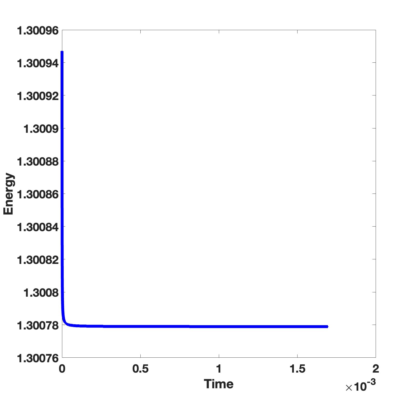
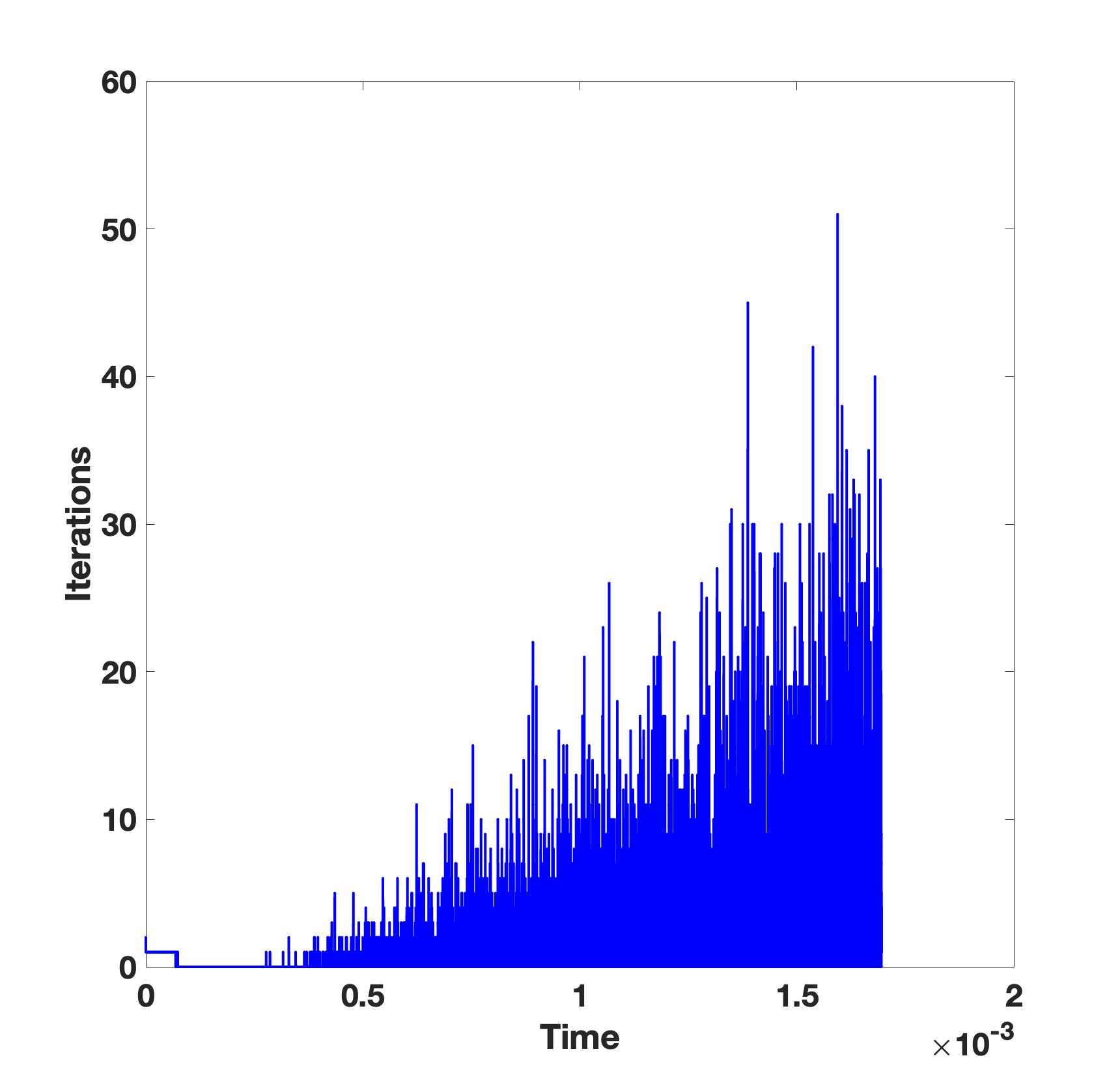
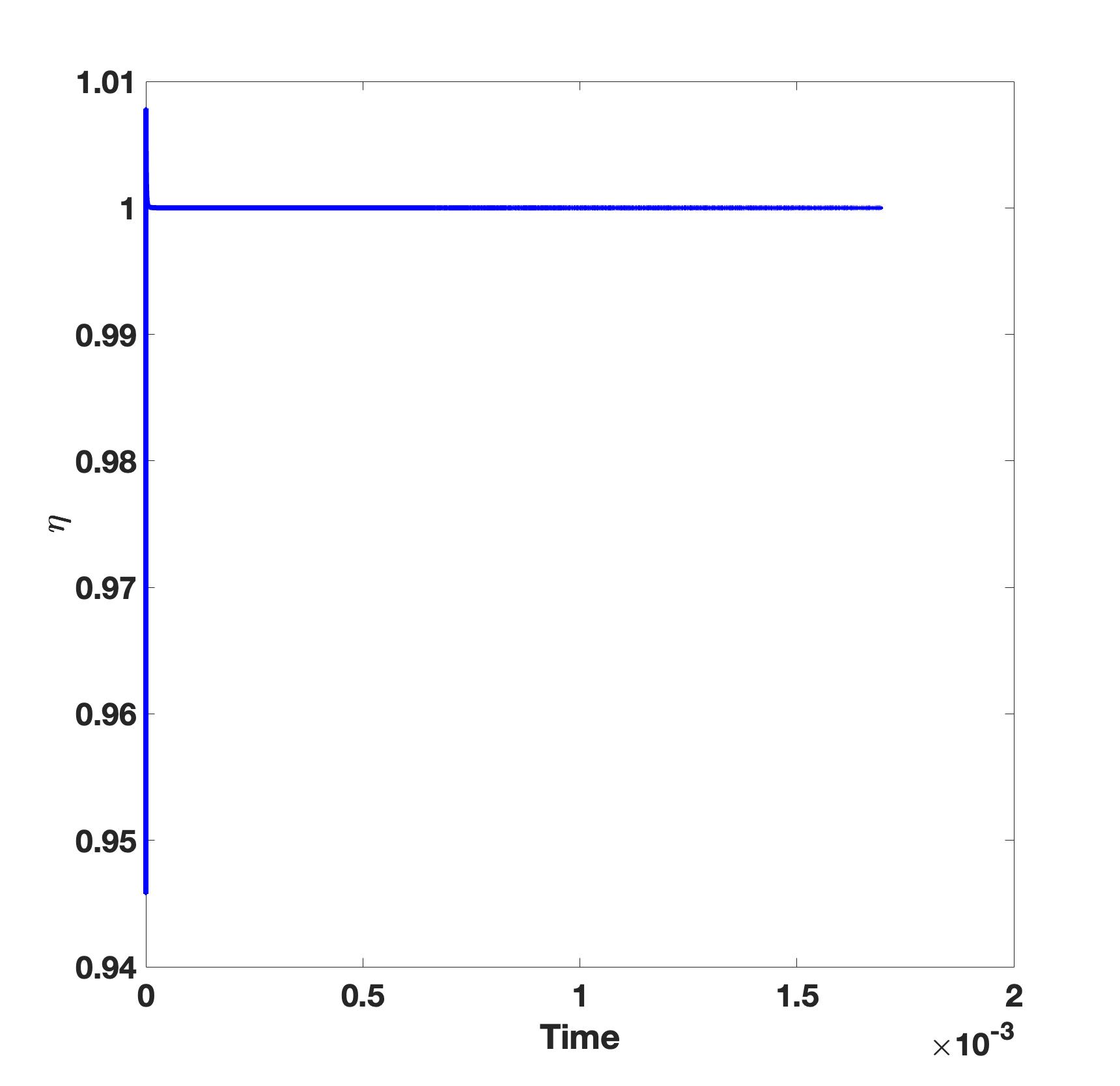
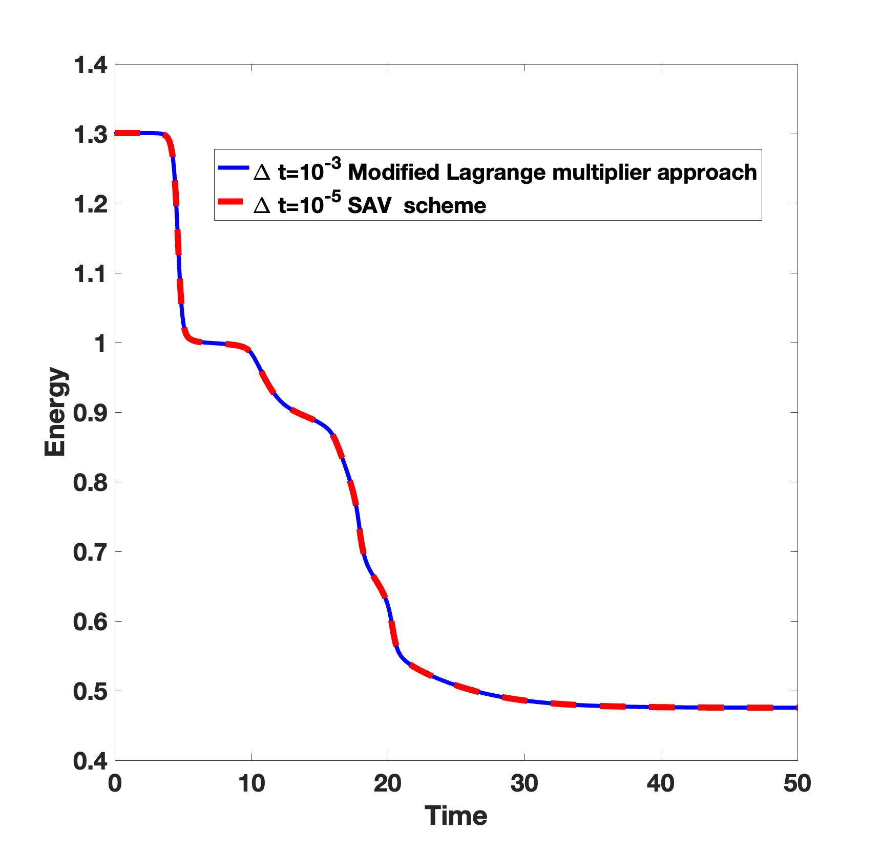
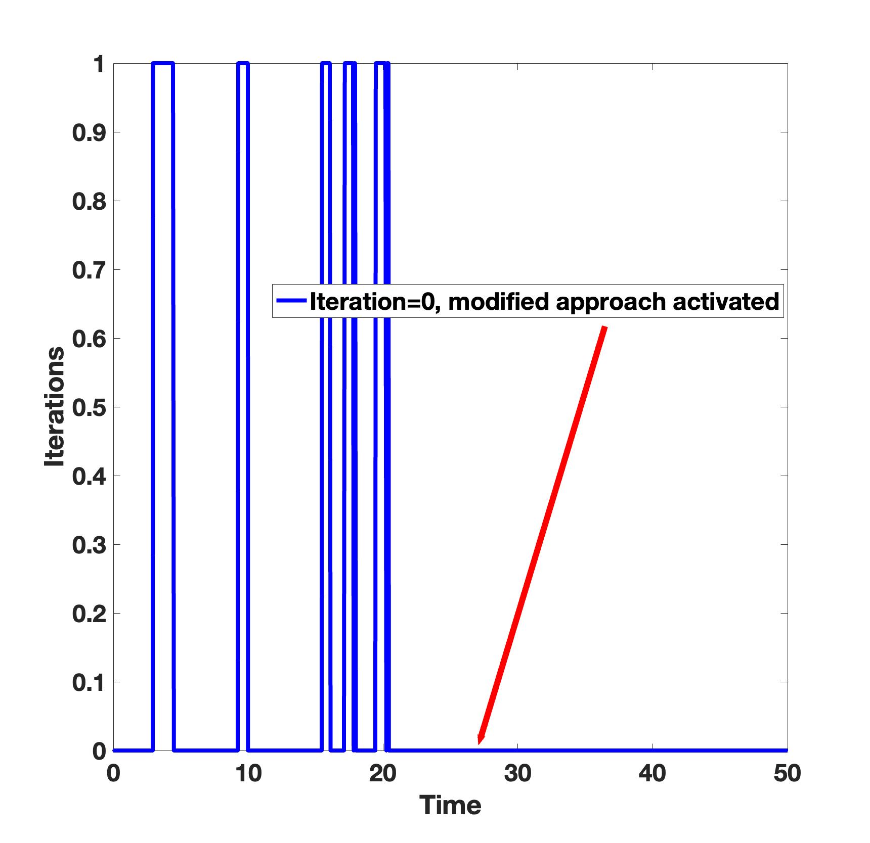
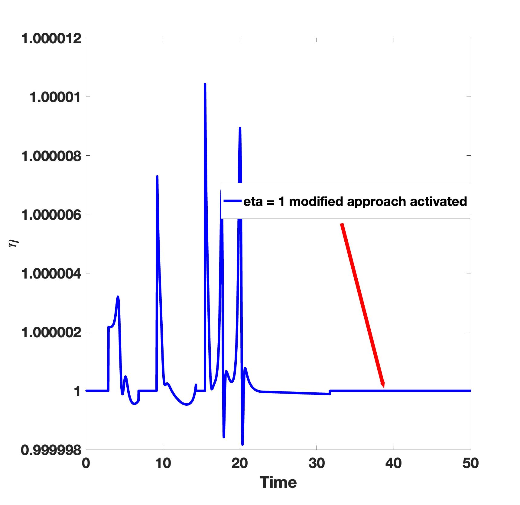
In Figure 1(a-c), we plot the evolution of energy, iterations and with respect to time by using the modified Crank-Nicolson scheme based on the original Lagrange multiplier approach. We observe that even with a very small time step , the scheme based on the original Lagrange multiplier approach failed to converge at about . In Figure 1(d-f), we plot the evolution of energy, iterations and with respect to time by using the scheme based on the modified Lagrange multiplier approach with and . For the sake of comparison, we also plot the energy evolution by using a second-order SAV scheme with . We observe from Figure 1(d) that the energy curves obtained by both methods overlap and decrease monotonically, indicating that the modified Lagrange multiplier approach leads to correct results ever at a relatively large time step . We also observe from Figure 1(e) that the modified approach is activated (i.e., ) in a large time interval, while only one iteration is needed for solving the nonlinear algebraic equation (2.15) when . These results indicate that the modified Lagrange multiplier approach is very effective.
(a)Energy with
(b)Iterations with
(c) with
(d)Energy with
(e)Iterations with
(f) with
Figure 1: (a-c): The evolution of energy, iterations and using the original Lagrange multiplier approach with . (d-f): The evolution of energy, iterations and using modified Lagrange multiplier approach with .
In this section, we provide the unique solvability analysis of (3.23). To fix the idea, we consider the Cahn-Hilliard equation, a typical gradient flow. In this physical model, the energy functional is given by
(3.18)
where the constant stands for the interface width parameter, and . In turn, the Cahn-Hilliard equation can be written as
(3.19)
in which is the chemical potential
(3.20)
For simplicity, periodic boundary conditions are imposed for both the phase variable, , and the chemical potential, . An extension to the case of homogeneous Neumann boundary condition would be straightforward.
In more details, the scheme (2.4)-(2.6) could be represented as
(3.21)
(3.22)
Meanwhile, the Lagrange multiplier is a solution of the nonlinear algebraic equation
We aim to provide a theoretical analysis for the nonlinear algebraic equation (3.23), by making use of certain localized estimates.
The numerical error function is defined as
(3.26)
in which is the exact solution to the original PDE (3.19), and is denoted as the numerical solution of (3.21)-(3.22). With an initial data with sufficient regularity, it is assumed that the exact solution has regularity of class :
(3.27)
In turn, the following functional bounds are available for the exact solution:
(3.28)
To proceed with the nonlinear analysis for (3.23), we begin with the following a priori assumption for the numerical error at the previous time steps:
(3.29)
In turn, the following and bounds are valid for the numerical solution at the previous time steps:
(3.30)
In particular, by the fact that , we have the following a-priori bounds for :
(3.31)
The a priori assumption (3.29) will be recovered by the convergence estimate at the next time step, as will be demonstrated in the later analysis.
The following theorem is the main result of this section.
Theorem 3.1.
Suppose the exact solution for the Cahn-Hilliard equation (3.19), of regularity class , satisfies the assumption (1.3) with . We also make the a-priori assumption (3.29). Then the nonlinear scalar equation (3.23) has a unique solution in .
We note that the numerical results presented in the last Section indicate that the condition (i.e. ) is most likely too pessimistic.
A few preliminary estimates are needed before we can proceed with the proof of this theorem.
3.2 Some preliminary estimates
For the sake of simplicity, we remove the dependent on from all constants below.
Lemma 3.1.
Given , . Under the assumption (1.3) and the a-priori assumption (3.29), we have the following estimates:
(3.32)
(3.33)
(3.34)
(3.35)
(3.36)
in which () only depends on .
Proof.
By the representation formula (3.24) for , we see that
(3.37)
(3.38)
Meanwhile, by the a priori estimate (3.30) for the numerical solution , , we have
(3.39)
On the other hand, the following inequality is always available, because all the eigenvalues associated with the operator is bounded by 1:
(3.40)
Then we arrive at
(3.41)
(3.42)
Therefore, an application of 3-D Sobolev embedding implies that
(3.43)
with the elliptic regularity used in the second step. In turn, the first inequality of (3.32) has been proved by taking .
The proof of the second inequality in (3.32) is more straightforward:
provided that . Again, the elliptic regularity has been recalled in the second step. As a result, the proof for second inequality in (3.32) is complete, by taking .
For the third inequality in (3.32), we begin with the following expansion, based on the fact that :
(3.44)
In turn, a combination of Hölder inequality and Sobolev embedding implies that
(3.45)
A similar estimate could also be derived; the details are skipped for the sake of brevity:
(3.46)
As a consequence, we arrive at
Furthermore, its combination with the a priori bound (3.31) (for ) results in
and an application of Sobolev embedding yields
This finishes the proof of the third inequality in (3.32), by taking .
The rest inequalities in (3.32)-(3.36) could be analyzed in the same fashion. The details are skipped for simplicity of presentation.
We aim to prove that the nonlinear equation (3.23) has a unique solution in a neighborhood of . An estimate of the value for is given by the following lemma.
Lemma 3.2.
Given , , under the assumption (1.3) and the a priori assumption (3.29), we have , with only depending on .
Proof.
We begin with the expansion of :
(3.47)
An application of intermediate value theorem implies that
As a consequence, we get
(3.48)
By the inequality (3.32), the following estimate is available:
(3.49)
Moreover, since is between and , we see that
(3.50)
Meanwhile, the following inequalities are available:
in which the regularity assumption (3.28) and the a priori assumption (3.29) have been applied. This in turn yields
(3.51)
To obtain a bound for , we observe that
(3.52)
which comes from the range of and . Meanwhile, by the fact that , the following bounds could be derived:
(3.53)
(3.54)
(3.55)
in which the a-priori bounds (3.30)-(3.31) have been repeatedly applied, and the last step of (3.55) is based on the following estimate:
provided that , . In addition, a careful calculation reveals that
(3.75)
A further decomposition is made to facilitate the later analysis:
(3.76)
An estimate for is straightforward:
so that
(3.77)
in which the fact that has been applied in the last step. For the part , we observe that (satisfied by the original PDE), so that a further decomposition is available:
We can now proceed to the proof of Theorem 3.1.
Without loss of generality, we assume that and , as the other cases could be analyzed in the same way. By Lemmas 3.2 and 3.3, we have
(3.82)
Then we conclude that, is monotone and increasing over the interval , with , so that
(3.83)
Therefore, there is a unique solution for over the interval . In addition, we have , if with . Since is increasing over , such a solution is unique in the interval . The proof is completed.
4 Error analysis
Given a tolerance , we shall assume
(4.84)
which implies in particular that for all .
Usually, the above assumption is only satisfied for , but for the sake of simplicity we shall assume . An error analysis is carried out in this section for the scheme (3.21)-(3.22) under the above assumption. For the time intervals where (4.84) is not satisfied, we use the modified Lagrange multiplier approach by setting and computing by (3.21).
The main result of this section is stated in the following theorem.
Theorem 4.1.
Given initial data , suppose the exact solution for the Cahn-Hilliard equation (3.19) is of regularity class ,
and satisfies the assumption (1.3). Then, provided that , we have
(4.85)
for all positive integers , such that , where are some positive constants independent of and .
The proof of this theorem will be carried out through a series of intermediate estimates which we describe below.
4.1 Energy stability and the estimate
The following result could be proved in a straightforward way.
Lemma 4.1.
If the numerical system (3.21)-(3.22) is solvable, it is energy stable with respect to the modified energy functional: , i.e., the following energy inequality holds:
Going back (4.87), we arrive at the desired inequality (4.86).
As a result of this result, we obtain a uniform bound of the original energy functional , for any :
Meanwhile, since , we get
And also, the numerical solution (3.21)-(3.22) is mass conservative, so that
In turn, an application of Poincaré inequality yields a uniform in time bound for the numerical solution:
(4.88)
We notice that is uniform in time, while it depends on in a polynomial pattern.
4.2 The estimate for the numerical solution
Lemma 4.2.
Under the assumption (1.3) with and the a priori assumption (3.29), we have
(4.89)
in which depends on in a polynomial pattern, while it is independent on and .
Proof.
First, it is noticed that, by the assumptions and Theorem 3.1, the scheme (3.21)-(3.22) has a unique solution in .
Taking an inner product with (3.21) by , we obtain
(4.90)
The inner product associated surface diffusion could be analyzed as follows:
For the right hand side in (4.90), we recall the expansion (3.44) and apply the Hölder inequality:
(4.91)
Meanwhile, the following estimates are available, based on Sobolev embedding and weighted inequalities, as well as the uniform in time estimate (4.88):
In turn, an application of Cauchy inequality implies that
(4.96)
in which the Young’s inequality has been extensively applied in the fourth step, and the last step is based on the fact that . We also notice that depends on and in a polynomial pattern.
Subsequently, a substitution of (4.2) and (4.96) into (4.90) leads to
In fact, this inequality could be rewritten as
With an introduction of a modified energy
we get
in which the following elliptic regularity has been used:
An application of the induction argument implies that
Of course, we could introduce a uniform in time quantity , so that for any . In turn, an application of the elliptic regularity reveals that
in which the uniform in time constant depends on in a polynomial pattern. This finishes the proof of Proposition 4.2.
Using similar tools, a uniform-in-time bound for the numerical solution could be established, for any , by taking inner product with (3.21) by , and performing the associated estimates. The details are left to interested readers.
Lemma 4.3.
Under the assumptions of Lemma 4.2, we have for any ,
(4.97)
in which depends on in a polynomial power, while it is independent on and .
4.3 Estimate for
The following estimate is needed in the later analysis.
By the expansion for , the following estimates could be derived, helped by repeated applications of the Hölder inequality and Sobolev embedding:
(4.100)
(4.101)
with the uniform-in-time estimates (4.97) used. Consequently, a substitution of (4.100)-(4.101) into (4.99) yields
Note that depends on in a polynomial form, since both and do as well. This completes the proof of Proposition 4.3.
4.4 A refined estimate for
An estimate have been derived for in Theorem 3.1. In fact, by the estimate (3.82), we see that
(4.102)
Again, this rough estimate is not sufficient for an optimal rate of convergence. We aim to improve this estimate so that . The following preliminary lemma is needed.
where is a constant independent of , dependent on the exact solution and .
Proof.
A careful calculation reveals that
in which the representation formulas (3.25), (3.37) have been applied.
For the first part of (4.4), we see that , and the following estimates could be derived by (4.97) :
(4.105)
(4.106)
in which the 3-D Sobolev embedding and Hölder inequality have been extensively applied, as well as the fact that . Then we arrive at
(4.107)
This in turn leads to
For the second part of (4.4), we make use of the following expression of (which comes from the numerical scheme (3.21)):
(4.108)
For the first part of the expansion (4.108), from (4.89) we have
(4.109)
Its combination with the preliminary rough estimate (4.102) implies that
(4.110)
For the second part of the expansion (4.108), we begin with the following identify:
(4.111)
In turn, extensive applications of Hölder inequality and Sobolev inequality indicate that
(4.112)
in which the estimate (4.89) and the discrete temporal derivative estimate (4.98) have been applied in the last step. For the third part of the expansion (4.108), we make use of (4.98) again, and get
(4.113)
Therefore, a substitution of (4.110), (4.112) and (4.113) into (4.108) leads to the following estimate:
(4.114)
Finally, a combination of (4.4), (4.106) and (4.114) yields the desired result (4.103), by taking . This finishes the proof of Lemma 4.5.
As a consequence, we are able to obtain a sharper estimate for , in comparison with Lemma 3.2.
Lemma 4.6.
Under the assumptions of Lemma 4.2, we have , with a constant independent of , but dependent on the exact solution .
For the part, we make use of the following identity
In turn, with an application of Hölder inequality, combined with the inequalities (3.32), (3.49), we obtain
(4.116)
For the part, we begin with the following application of intermediate value theorem:
with between and . By the fact that and the bounds for and , we get
Then we arrive at
(4.117)
in which the estimate (4.103) (in Lemma 4.5) has been applied in the second step. Therefore, a combination of (4.115), (4.116) and (4.117) yields the desired result, by taking . This finishes the proof of Lemma 4.6.
Next, we have to obtain a refined estimate for .
Lemma 4.7.
Under the assumptions of Lemma 4.2, we have with dependent on the exact solution .
Proof.
Again, it is assumed that , without loss of generality. Following the proof of Theorem 3.1, we see that
Then we conclude that, is monotone and increasing over the interval , with , so that
Therefore, there is a unique solution for over the interval . This finishes the proof of Theorem 4.7.
4.5 Proof of Theorem 4.1
First of all, it is clear that both the exact solution and the numerical solution are mass conservative:
(4.118)
in which is the exact solution evaluated at the time instant . Then we conclude that the numerical error function must have zero-average at each time step:
(4.119)
In turn, the following elliptic regularity estimates are available:
(4.120)
First, the a priori assumption (3.29) is made. As a result, the unique solvability for (in the range of ) is assured by Theorem 3.1, and a refined estimate in Lemma 4.7 becomes available.
The following truncation error analysis for the exact solution can be obtained by using a straightforward Taylor expansion:
(4.121)
with .
In turn, subtracting the numerical scheme (3.21) from the consistency estimate (4.121) yields
in which the integration by parts have been extensively applied in the derivation. The surface diffusion term could be analyzed similarly as in (4.2):
The local truncation error term could be bounded by the Cauchy inequality:
(4.124)
For the first nonlinear inner product, we recall the refined estimate, , as established in Lemma 4.7. In addition, the following estimate could be derived:
(4.125)
based on the fact that , and the bound (3.28) for the exact solution. Then we arrive at
(4.126)
For the other nonlinear error term, we begin with the following application of intermediate value theorem:
This in turn leads to the following estimate:
Consequently, the following inequality is available:
with . Therefore, an application of discrete Gronwall inequality yields the desired convergence estimate (4.85).
Finally, we have to recover the a-priori assumption (3.29) at time step to close the induction argument. By the convergence estimate (4.85), we get
Making use of the elliptic regularity estimate (4.120), we have
Therefore, the a-priori assumption (3.29) is valid at time step , provided that
This finishes the complete induction argument for both the solvability analysis and convergence estimate.
5 Concluding remarks
The unique solvability and error analysis of the original Lagrange multiplier approach, proposed in [8] for gradient flows, is considered in this article. We first identified a necessary and sufficient condition that must be satisfied for the system of nonlinear algebraic equations, arising from the original Lagrange multiplier approach, to admit a unique solution in the neighborhood of its exact solution. Afterward, we proposed a modified Lagrange multiplier approach to ensure that the computation can continue even if the aforementioned condition was not satisfied.
However, a globally unique solvability of the nonlinear system of algebraic equations is not possible, due to the non-monotone feature of the implicit part in the numerical system. Using the Cahn-Hilliard equation and a second-order modified Crank-Nicholson scheme with a Lagrange multiplier as an example, we have provided a unique solvability analysis using localized estimates in the neighborhood of its exact solution under an a-priori assumption, and then carried out a rigorous error analysis, which in turn recovered the a-priori assumption using an inductive argument.
The results presented in this paper are the first unique solvability analysis and error estimate for the original Lagrange multiplier approach. In a future work, we shall consider the theoretical analysis for a more general Lagrange multiplier approach for gradient flows with global constraints proposed in [9]. Due to the multiple Lagrange multipliers involved in the latter approach, the analysis would be much more challenging, while the analytical techniques introduced in this paper may be helpful.
Acknowledgements
This work is supported in part by NSFC 12371409 (J. Shen), NSFC 12301522 (Q. Cheng) and NSF DMS-2012269, DMS-2309548 (C. Wang).
References
[1]
X. Antoine, J. Shen, and Q. Tang.
Scalar auxiliary variable/Lagrange multiplier based pseudospectral
schemes for the dynamics of nonlinear Schrödinger/Gross-Pitaevskii
equations.
J. Comput. Phys., 437:Paper No. 110328, 19, 2021.
[2]
A. Aristotelous, O. Karakasian, and S.M. Wise.
A mixed discontinuous Galerkin, convex splitting scheme for a
modified Cahn-Hilliard equation and an efficient nonlinear multigrid
solver.
Discrete Contin. Dyn. Sys. B, 18:2211–2238, 2013.
[3]
W. Bao and Q. Du.
Computing the ground state solution of bose–einstein condensates by
a normalized gradient flow.
SIAM J. Sci. Comput., 25(5):1674–1697, March 2004.
[4]
W. Chen, C. Wang, X. Wang, and S.M. Wise.
Positivity-preserving, energy stable numerical schemes for the
Cahn-Hilliard equation with logarithmic potential.
J. Comput. Phys.: X, 3:100031, 2019.
[5]
K. Cheng, W. Feng, C. Wang, and S.M. Wise.
An energy stable fourth order finite difference scheme for the
Cahn-Hilliard equation.
J. Comput. Appl. Math., 362:574–595, 2019.
[6]
K. Cheng, C. Wang, S.M. Wise, and Y. Wu.
A third order accurate in time, BDF-type energy stable scheme for
the Cahn-Hilliard equation.
Numer. Math. Theor. Meth. Appl., 15(2):279–303, 2022.
[7]
K. Cheng, C. Wang, S.M. Wise, and X. Yue.
A second-order, weakly energy-stable pseudo-spectral scheme for the
Cahn-Hilliard equation and its solution by the homogeneous linear iteration
method.
J. Sci. Comput., 69:1083–1114, 2016.
[8]
Q. Cheng, C. Liu, and J. Shen.
A new lagrange multiplier approach for gradient flows.
Comput. Methods Appl. Mech. Engrg., 367:13070, 2020.
[9]
Q. Cheng and J. Shen.
Global constraints preserving scalar auxiliary variable schemes for
gradient flows.
SIAM J. Sci. Comput., 42:A2514–A2536, 2020.
[10]
A. Diegel, C. Wang, and S.M. Wise.
Stability and convergence of a second order mixed finite element
method for the Cahn-Hilliard equation.
IMA J. Numer. Anal., 36:1867–1897, 2016.
[11]
L. Dong, C. Wang, S.M. Wise, and Z. Zhang.
A positivity-preserving, energy stable scheme for a ternary
Cahn-Hilliard system with the singular interfacial parameters.
J. Comput. Phys., 442:110451, 2021.
[12]
L. Dong, C. Wang, S.M. Wise, and Z. Zhang.
Optimal rate convergence analysis of a numerical scheme for the
ternary Cahn-Hilliard system with a Flory-Huggins-deGennes energy
potential.
J. Comput. Appl. Math., 406:114474, 2022.
[13]
L. Dong, C. Wang, H. Zhang, and Z. Zhang.
A positivity-preserving, energy stable and convergent numerical
scheme for the Cahn-Hilliard equation with a Flory-Huggins-deGennes
energy.
Commun. Math. Sci., 17:921–939, 2019.
[14]
Q. Du and F. Lin.
Numerical approximations of a norm-preserving gradient flow and
applications to an optimal partition problem.
Nonlinearity, 22(1):67–83, December 2008.
[15]
Q. Du, C. Liu, and X. Wang.
Simulating the deformation of vesicle membranes under elastic bending
energy in three dimensions.
J. Comput. Phys., 212(2):757–777, March 2006.
[16]
C.M. Elliott and A.M. Stuart.
The global dynamics of discrete semilinear parabolic equations.
SIAM J. Numer. Anal., 30:1622–1663, 1993.
[17]
D. Eyre.
Unconditionally gradient stable time marching the Cahn-Hilliard
equation.
In J. W. Bullard, R. Kalia, M. Stoneham, and L.Q. Chen, editors, Computational and Mathematical Models of Microstructural Evolution,
volume 53, pages 1686–1712, Warrendale, PA, USA, 1998. Materials Research
Society.
[18]
J. Guo, C. Wang, S.M. Wise, and X. Yue.
An convergence of a second-order convex-splitting, finite
difference scheme for the three-dimensional Cahn-Hilliard equation.
Commu. Math. Sci., 14:489–515, 2016.
[19]
J. Guo, C. Wang, S.M. Wise, and X. Yue.
An improved error analysis for a second-order numerical scheme for
the Cahn-Hilliard equation.
J. Comput. Appl. Math., 388:113300, 2021.
[20]
L. Ju, X. Li, and Z. Qiao.
Generalized SAV-exponential integrator schemes for Allen-Cahn
type gradient flows.
SIAM J. Numer. Anal., 60(4):1905–1931, 2022.
[21]
L. Ju, X. Li, and Z. Qiao.
Stabilized exponential-SAV schemes preserving energy dissipation
law and maximum bound principle for the Allen-Cahn type equations.
J. Sci. Comput., 92(2):Paper No. 66, 34, 2022.
[22]
D. Li and Z. Qiao.
On second order semi-implicit Fourier spectral methods for 2D
Cahn-Hilliard equations.
J. Sci. Comput., 70:301–341, 2017.
[23]
D. Li and Z. Qiao.
On the stabilization size of semi-implicit Fourier-spectral methods
for 3D Cahn-Hilliard equations.
Commun. Math. Sci., 15:1489–1506, 2017.
[24]
D. Li, Z. Qiao, and T. Tang.
Characterizing the stabilization size for semi-implicit
Fourier-spectral method to phase field equations.
SIAM J. Numer. Anal., 54:1653–1681, 2016.
[25]
J. Shen, J. Xu, and J. Yang.
The scalar auxiliary variable (SAV) approach for gradient flows.
J. Comput. Phys., 353:407–416, 2018.
[26]
J. Shen, J. Xu, and J. Yang.
A new class of efficient and robust energy stable schemes for
gradient flows.
SIAM Review, 61(3):474–506, 2019.
[27]
J. Shen and X. Yang.
Numerical approximations of Allen-Cahn and Cahn-Hilliard
equations.
Discrete Contin. Dyn. Sys. A, 28:1669–1691, 2010.
[28]
Y. Yan, W. Chen, C. Wang, and S.M. Wise.
A second-order energy stable BDF numerical scheme for the
Cahn-Hilliard equation.
Commun. Comput. Phys., 23:572–602, 2018.
[29]
X. Yang, J. Zhao, Q. Wang, and J. Shen.
Numerical approximations for a three components Cahn-Hilliard
phase-field model based on the invariant energy quadratization method.
M3AS: Mathematical Models and Methods in Applied Sciences,
27(11), August 2017.
[30]
M. Yuan, W. Chen, C. Wang, S.M. Wise, and Z. Zhang.
An energy stable finite element scheme for the three-component
Cahn-Hilliard-type model for macromolecular microsphere composite
hydrogels.
J. Sci. Comput., 87:78, 2021.