Hall effect on the joint cascades of magnetic energy and helicity in helical magnetohydrodynamic turbulence

Abstract

Helical magnetohydrodynamic turbulence with Hall effects is ubiquitous in heliophysics and plasma physics, such as star formation and solar activities, and its intrinsic mechanisms are still not clearly explained. Direct numerical simulations reveal that when the forcing scale is comparable to the ion inertial scale, Hall effects induce remarkable cross helicity. It then suppresses the inverse cascade efficiency, leading to the accumulation of large-scale magnetic energy and helicity. The process is accompanied by the breaking of current sheets via filaments along magnetic fields. Using the Ulysses data, the numerical findings are separately confirmed. These results suggest a novel mechanism wherein small-scale Hall effects could strongly affect large-scale magnetic fields through cross helicity.

In Hall magnetohydrodynamic (HMHD) turbulence, the ions and electrons decouple from each other, which can be modeled via the Hall term in the generalized Ohm’s law (Galtier, 2016). HMHD model is valid for the process with timescales shorter than the ion cyclotron period, such as star formation (Marchand et al., 2019; Norman and Heyvaerts, 1985; Wurster et al., 2021), dynamo action (Gómez et al., 2010; Mininni et al., 2005), planetary magnetosphere (Dorelli et al., 2015), and solar activities (Bhattacharjee, 2004; Cassak et al., 2005). In the solar corona, the strongly helical magnetic field collisionlessly reconnects, leading to the rapid eruption of plasma (Ebrahimi and Raman, 2015; Wan et al., 2015; Faganello et al., 2008; Servidio et al., 2009; Sun et al., 2022).

In solar wind observation, the turbulent nature can be verified through the von Kármán-Howarth (vKH) relations for magnetohydrodynamic (MHD) turbulence (De Karman and Howarth, 1938; Politano and Pouquet, 1998; Marino et al., 2011, 2012; Sorriso-Valvo et al., 2007). Based on vKH relations, Smith et al. (2009) discovered prevailing inverse energy cascades when the cross helicity is pronounced. Marino et al. (2012) found that cross helicity could affect the linear scaling ratio of the vKH relation. In MHD and HMHD turbulence, magnetic helicity is another conservative quantity besides energy, and could measure the magnetic reconnection process quantitatively (Galtier, 2016). Politano et al. (2003) derived the vKH relations for magnetic helicity in MHD turbulence. Banerjee and Galtier (2016) derived the balance for magnetic helicity in HMHD turbulence. Brandenburg et al. (2011) found the sign change of magnetic helicity at small- and large-scale solar wind.

In practice, even if solar wind can be described by MHD turbulence, the detailed mechanisms are hard to be investigated in actual space plasma due to its complex nature. High-precision direct numerical simulations (DNS) are necessary. DNS of the helical MHD turbulence showed that helicity injection could lead to the formation of a large-scale magnetic field (Müller et al., 2012; Richner et al., 2022). Mininni et al. (2005) found the faster growth rates of large-scale magnetic fields in HMHD turbulence. Dreher et al. (2005) studied the formation and disruption of Alfvénic filaments under Hall effects.

However, even if there have been separate studies on magnetic helicity and Hall effects, there remains limited researches on their coupling effects, which are significant in the collisionless reconnection of the solar corona (Ebrahimi and Raman, 2015). The vKH relation about the magnetic helicity in HMHD turbulence is still not addressed, and the existing related theoretical works are also not verified. In this letter, we will investigate the Hall effects on the cascades of magnetic energy and helicity, and then verify those findings based on vKH relations in actual solar wind.

The governing equations for the velocity $\bf v$ and the magnetic field $\bf b$ are (Marino and Sorriso-Valvo, 2023; Müller et al., 2012):

$$\partial_{t}{\bf v} =-({\bf v}\cdot{\bf\nabla}){\bf v}-{\bf\nabla}p+{\bf j}\times{\bf b}+\lambda\Delta^{-1}{\bf v}+\nu\Delta{\bf v}+{\bf f_{v}},$$ (1)

$$\partial_{t}{\bf b} =\nabla\times({\bf U}\times{\bf b})+\lambda_{b}\Delta^{-1}{\bf b}+\eta\Delta{\bf b}+{\bf f_{b}},$$

where $\nabla\cdot{\bf v}=0$ and $\nabla\cdot{\bf b}=0$, $p$ is the pressure, ${\bf U}={\bf v}-d_{I}{\bf j}$, $d_{I}$ is the ion inertial length, ${\bf j}=\nabla\times{\bf b}$ is the current density, ${\bf f_{v}}$ and ${\bf f_{b}}$ are forcing terms at forcing wavenumbers $k_{f}$, $\lambda\Delta^{-1}{\bf v}$ and $\lambda_{b}\Delta^{-1}{\bf b}$ are hypo-viscous terms, $\nu$ and $\eta$ are the kinematic viscosity and magnetic diffusivity, respectively.

Six DNSs are performed in this letter. The computational parameters are shown in TABLE 1. M3, M6 and M40 are the MHD cases with different $k_{f}$, while H3, H6 and H40 are corresponding HMHD cases. The random forcing schemes (${\bf f_{v}}$ and ${\bf f_{b}}$) only inject maximum magnetic helicity artificially but do not inject any hydrodynamic or cross helicity. See the Supplemental Material (SM) (sup, ) for more numerical details.

Table 1: The computational configurations of flows. $\varepsilon_{v}$ and $\varepsilon_{b}$ are injection rates of hydrodynamic and magnetic energy.

Case	Grid	$d_{I}$	$\nu=\eta$	$\lambda=\lambda_{b}$	$k_{f}$	$\varepsilon_{v}=\varepsilon_{b}$
M3	$2048^{3}$	–	$4\times 10^{-5}$	0.1	3	0.015
H3	$2048^{3}$	0.05	$4\times 10^{-5}$	0.1	3	0.015
M6	$2048^{3}$	–	$4\times 10^{-5}$	0.1	6	0.015
H6	$2048^{3}$	0.05	$4\times 10^{-5}$	0.1	6	0.015
M40	$1024^{3}$	–	$10^{-4}$	0.05	40-42	0.015
H40	$1024^{3}$	0.05	$10^{-4}$	0.05	40-42	0.015

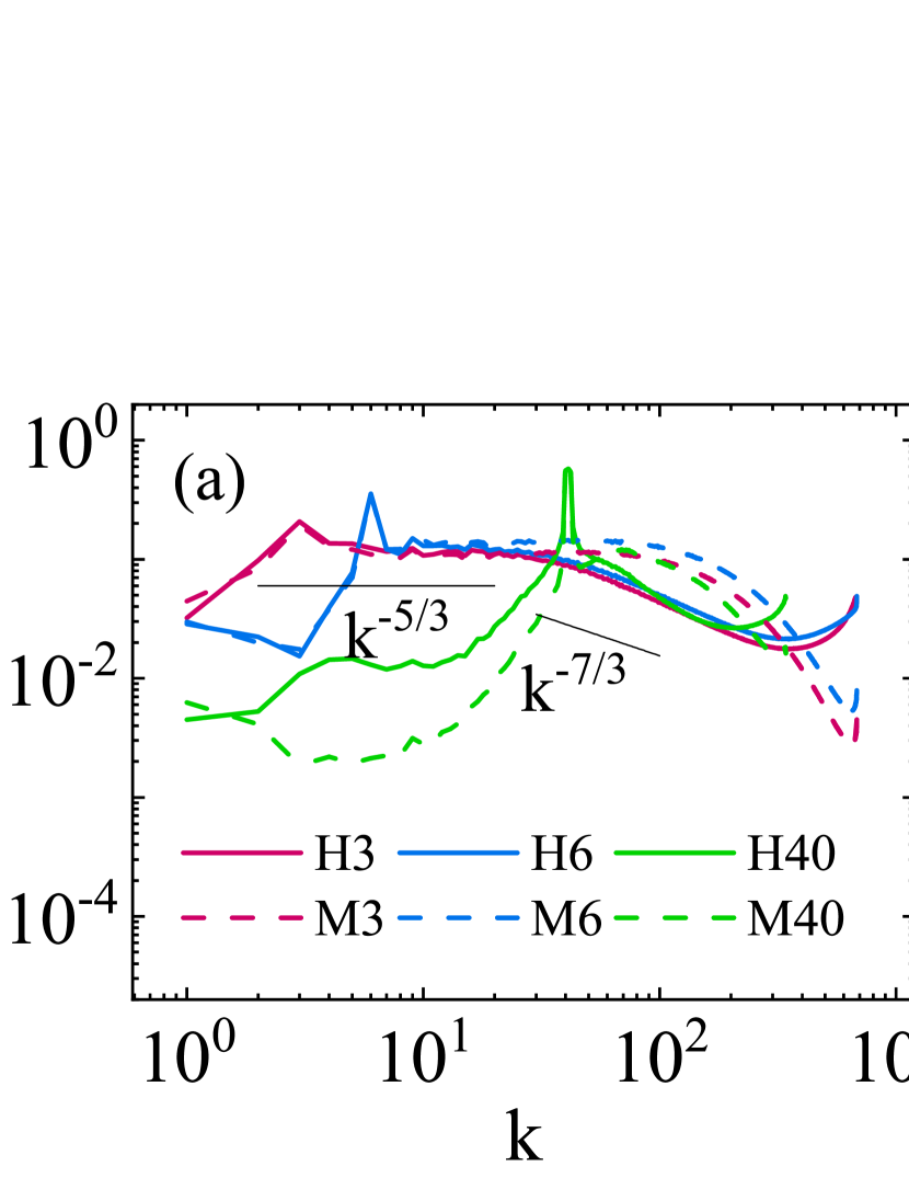
Figure 1: Compensated Spectra. (a) $E_{b}(k)k^{5/3}$. (b) $H_{M}(k)k^{10/3}$.

FIG. 1 shows the spectra of magnetic energy $E_{b}(k)=\sum_{|{\bf k}|=k}\Re\{\hat{\bf b}({\bf k})\cdot\hat{\bf b}^{\ast}({\bf k})\}/2$ and magnetic helicity $H_{M}(k)=\sum_{|{\bf k}|=k}\Re\{\hat{\bf a}({\bf k})\cdot\hat{\bf b}^{\ast}({\bf k})\}$, where $\hat{\cdot}$ represents the values in spectral space, and $\hat{\bf a}({\bf k})$ is the magnetic potential. In FIG. 1 (a), $E_{b}(k)\sim k^{-5/3}$ in the inertial range ($k\in(4,100)$), but in the ion inertial scale ($k\sim 1/d_{I}$), $E_{b}(k)\sim k^{-7/3}$ for HMHD cases (H3 and H6). For the magnetic helicity in FIG. 1 (b), $H_{M}(k)\sim k^{-10/3}$ for M3 and M6, due to the Alfvénic balance (Mininni and Pouquet, 2009). For the inverse cascade ranges of H40 and M40, $H_{M}(k)\sim k^{-8/3}\sim E_{b}(k)/k$, implying a fully helical magnetic field. In the evolutionary process given in SM (sup, ), $H_{M}(k)\sim k^{-10/3}$ in the inverse cascade range (Müller et al., 2012; Linkmann and Dallas, 2017). Furthermore, the comparison of M40 and H40 shows that Hall effects enhance large-scale magnetic energy and helicity by nearly tenfold. This implies Hall effects could strongly affect large-scale magnetic fields, which is the main subject of this letter.

Then, the filtering approach (Camporeale et al., 2018; Manzini et al., 2022) is used for the details of cascades. The fluxes for the magnetic energy ($\widetilde{\Pi}_{Eb1}$ and $\widetilde{\Pi}_{Eb2}$) and magnetic helicity ($\widetilde{\Pi}_{HM1}$ and $\widetilde{\Pi}_{HM2}$) are considered:

$$\widetilde{\Pi}_{Eb1} =-\epsilon_{ijk}\tilde{j}_{i}\tau_{jk}({\bf v},{\bf{b}}),$$ (2a)

$$\widetilde{\Pi}_{Eb2} =\epsilon_{ijk}d_{I}\tilde{j}_{i}\tau_{jk}({\bf j},{\bf b}),$$ (2b)

$$\widetilde{\Pi}_{HM1} =-2\epsilon_{ijk}\tilde{b}_{i}\tau_{jk}({\bf v},{\bf b}),$$ (2c)

$$\widetilde{\Pi}_{HM2} =2\epsilon_{ijk}d_{I}\tilde{b}_{i}\tau_{jk}({\bf j},{\bf b}),$$ (2d)

where ${\bf\tau}_{ij}({\bf p},{\bf q})=\widetilde{{p_{i}q_{j}}}-\widetilde{{p}_{i}}\widetilde{{q}_{j}}$ for arbitrary vectors $\bf p$ and $\bf q$, and the superscript $\widetilde{\cdot}$ represents the filtered quantities. $\widetilde{\Pi}_{Eb1}$ and $\widetilde{\Pi}_{HM1}$ both appear in MHD and HMHD turbulence, while $\widetilde{\Pi}_{Eb2}$ and $\widetilde{\Pi}_{HM2}$ only appear in HMHD turbulence. The overall magnetic energy $\widetilde{\Pi}_{Eb}=\widetilde{\Pi}_{Eb1}+\widetilde{\Pi}_{Eb2}$, and the overall magnetic helicity $\widetilde{\Pi}_{HM}=\widetilde{\Pi}_{HM1}+\widetilde{\Pi}_{HM2}$. For filtering approaches, different filters lead to consistent qualitative results (Yan et al., 2020; Kuzzay et al., 2019), and the fourth-order Butterworth filter (Camporeale et al., 2018) is used in this study.

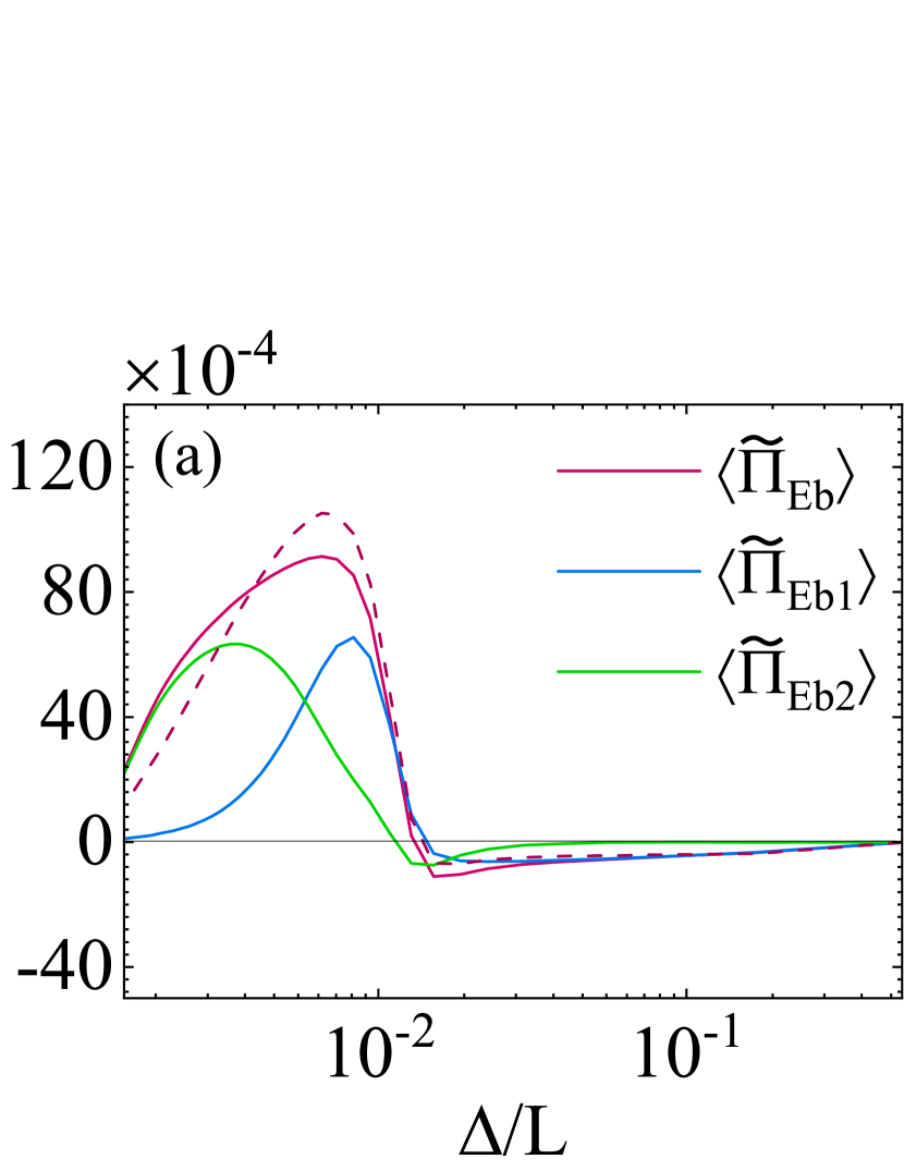
Figure 2: Fluxes versus the filter width $\Delta$, where $L=2\pi$. (a) Magnetic energy fluxes; (b) Magnetic helicity fluxes. Solid lines: H40; dashed lines: M40.

FIG. 2 (a) shows the magnetic energy fluxes of H40 and M40, where $\left\langle\cdot\right\rangle$ represents the ensemble average. As shown, most magnetic energy cascades forward towards small scales. Weak inverse cascades also appear and have been identified as the $\alpha$-effects (Müller et al., 2012; Linkmann and Dallas, 2017; Pouquet et al., 2019). FIG. 2 (b) shows the magnetic helicity fluxes. $\left\langle\widetilde{\Pi}_{HM1}\right\rangle$ is the dominant term, and most magnetic helicity cascades inversely towards large scales. Hall effects slightly reduce the inverse cascade rates, attributed to the far greater large-scale magnetic helicity and hypo-viscosity. In summary, Hall effects minimally affect the inverse cascades of magnetic energy and helicity in FIG. 2, but strongly enhance the large-scale magnetic energy and helicity in FIG. 1. Therefore, it can be inferred that the enhanced large-scale magnetic field may be related to the inefficiency of cascades.

With large scales governed by the inverse magnetic helicity cascades, the dominant term $\left\langle\widetilde{\Pi}_{HM1}\right\rangle$ is the focus henceforth. According to Eq. (1) and (2c), the cascade is directly related to cross helicity. FIG. 3 (a) shows the cross helicity spectra $H_{C}(k)=\sum_{|{\bf k}|=k}\Re\{\hat{\bf v}({\bf k})\cdot\hat{\bf b}^{\ast}({\bf k})\}$. As shown, $H_{C}(k)$ is approximately zero for MHD cases but negative for HMHD cases. In fact, for MHD cases, cross helicity is conservative (Galtier, 2016). No cross helicity is injected, making it inherently zero. In contrast, for HMHD cases, generalized helicity and magnetic helicity are conservative (Galtier, 2016). The generalized helicity can be decomposed into the sum of magnetic, hydrodynamic and cross helicity weighted by $d_{I}$. Therefore, the weighted sum of hydrodynamic and cross helicity is conservative. The hydrodynamic helicity is transformed to cross helicity through the Hall term ($d_{I}\nabla\times({\bf j}\times{\bf b})$). For the physical mechanisms, Hall effects are in fact the ion cyclotron effects on the magnetic field induced by the Lorentz force. In MHD cases, only the ion cyclotron effects on the velocity field are considered. In HMHD cases, the introduction of ion cyclotron effects on the magnetic field, which couples the chiralities of velocity and magnetic fields, produces non-zero cross helicity.

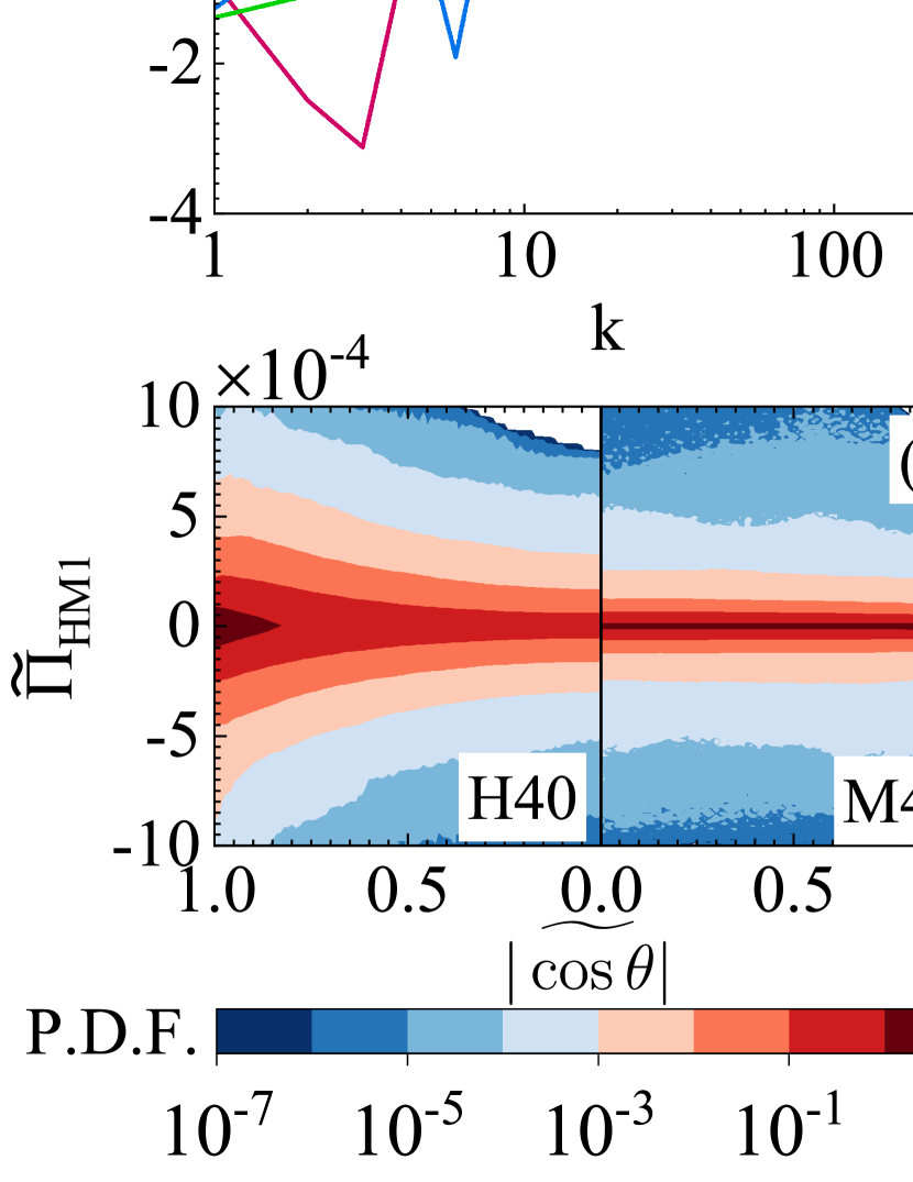
Figure 3: Cross helicity distributions and magnetic helicity cascades. (a) $H_{C}(k)$. (b) P.D.F. of $|\widetilde{\cos\theta}|$, with $\Delta_{1}=0.038L$ and $\Delta_{2}=0.013L$. Solid lines: H40; Dashed lines: M40. (c) Joint P.D.F. of $\widetilde{\Pi}_{HM1}$ and $|\widetilde{\cos\theta}|$ with $\Delta=0.038L$. (d) Conditional average of $\Gamma_{HM1}$ versus $|\widetilde{\cos\theta}|$, with $\Delta=0.038L$.

Furthermore, the normalized cross helicity can be defined as $\widetilde{\cos\theta}={\widetilde{{\bf v}}\cdot\widetilde{{\bf b}}}/[{|\widetilde{{\bf v}}||\widetilde{{\bf b}}|}]$, which evaluates the angle between velocity and the magnetic fields. The normalized cross helicity directly affects the cascade rates through the term $\nabla\times({\bf v}\times{\bf b})$ in Eq. (1) and $\widetilde{\Pi}_{Eb1}$,$\widetilde{\Pi}_{HM1}$ in Eq. (2). As $|\widetilde{\cos\theta}|$ increases, the velocity and magnetic fields align with each other, which could reduce the efficiency of $\widetilde{\Pi}_{Eb1}$,$\widetilde{\Pi}_{HM1}$. FIG. 3 (b) shows the probability distribution functions (P.D.F.) of $|\widetilde{\cos\theta}|$ with two filter widths $\Delta_{1}=0.038L$ and $\Delta_{2}=0.013L$. As the filter width increases or the Hall effects are introduced, $|\widetilde{\cos\theta}|$ centers around 1.0, indicating enhanced alignments between $\bf\widetilde{v}$ and $\bf\widetilde{b}$. FIG. 3 (c) compares the joint P.D.F. of $\widetilde{\Pi}_{HM1}$ and $\widetilde{\cos\theta}$ between H40 and M40 with the filter width $\Delta=0.038L$. For M40, $\widetilde{\Pi}_{HM1}$ are almost independent with $|\widetilde{\cos\theta}|$. In contrast, as Hall effects are introduced (H40), $\widetilde{\Pi}_{HM1}$ primarily concentrates on the region with significant $|\widetilde{\cos\theta}|$, indicating a potential decrease in efficiency. For a quantitative estimation, a direct definition of efficiency $\Gamma_{HM1}$ is introduced as

$$\Gamma_{HM1}=\frac{|\widetilde{\Pi}_{HM1}|}{2|\widetilde{\bf b}||\epsilon_{ijk}\tau_{jk}({\bf v},{\bf b}){\bf e}_{i}|}\frac{|\widetilde{\bf v}\times\widetilde{\bf b}|}{|\widetilde{\bf v}|\,|\widetilde{\bf b}|},$$ (3)

where ${\bf e}_{i}$ is the unit vector on the $i$-th direction, the first fraction evaluates the efficiency loss induced by the angle between the two vectors $\widetilde{\bf b}$ and $\epsilon_{ijk}\tau_{jk}({\bf v},{\bf b}){\bf e}_{i}$, and the second fraction evaluates the direct efficiency loss induced by the angle between $\widetilde{\bf v}$ and $\widetilde{\bf b}$. FIG. 3 (d) shows the conditional average $\left\langle\Gamma_{HM1}||\widetilde{\cos\theta}|\right\rangle$ with $\Delta=0.038L$. $\Gamma_{HM1}$ is inversely proportional to $|\widetilde{\cos\theta}|$. In addition, H40 has a relatively lower efficiency than M40. Specifically, when $\Delta=0.038L$, Hall effects reduce the averaged efficiency $\left\langle\Gamma_{HM1}\right\rangle$ by 53.2%.

In fact, both hydrodynamic helicity in hydrodynamic turbulence (Chen et al., 2003; Yan et al., 2020) and cross helicity in HMHD turbulence could affect cascade efficiencies. It could be of interest to investigate the disparities between the effects induced by the two helicity. Generally, hydrodynamic or cross helicity has two sources: geometric and phase alignments (Milanese et al., 2021). Taking the cross helicity as an example, geometric alignment means an increase in $|\widetilde{\cos\theta}|$, while phase alignment denotes a transformation from negative $\widetilde{\cos\theta}$ to positive $\widetilde{\cos\theta}$. Milanese et al. (2021) found that in hydrodynamic turbulence, hydrodynamic helicity cascades forward with dynamic phase alignments, while no geometry alignment is detected. In comparison, FIG. 3 (b) reveals that geometric alignments are the key processes in HMHD turbulence. The two different alignments lead to different effects on cascades. As shown in FIG. 3 (b-d), the geometric alignment induced by Hall effects strongly reduces the cascade efficiency.

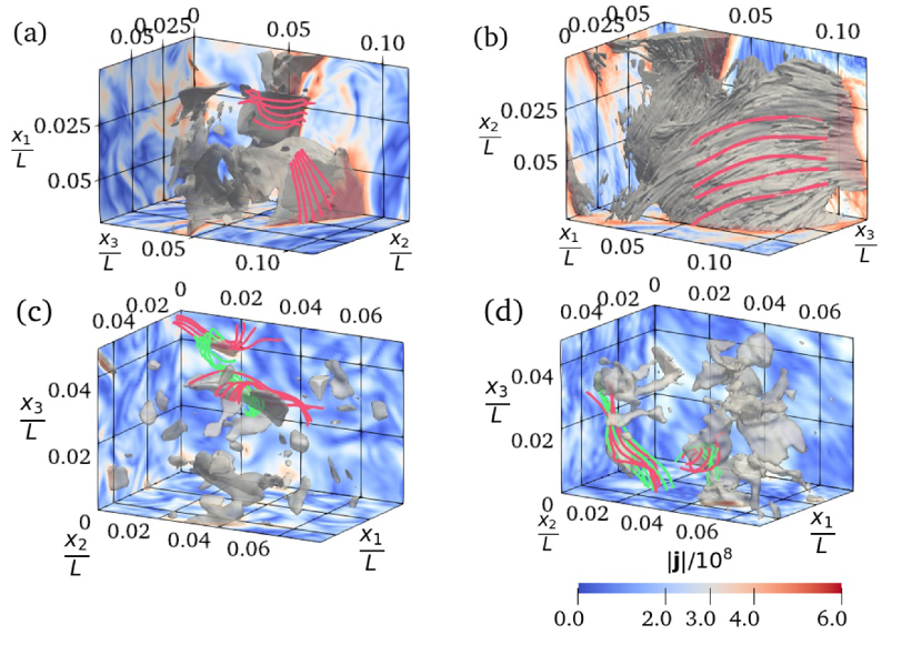
Figure 4: Structures with $|{\bf j}|>2.2\,\textrm{mean}\{|{\bf j}|\}$. The background slice shows the contour of $|{\bf j}|$. (a) M3; (b) H3; (c) M40; (d) H40. Pink lines: magnetic lines; Green lines: streamlines.

FIG. 4 shows the current density $|{\bf j}|$, where the pink and green lines give the magnetic lines and streamlines, respectively. The comparison of FIG. 4 (a) M3 and (b) H3 reveals that when the forcing scale is significantly larger than $d_{I}$, Hall effects induce filaments along the magnetic field (Miura and Hori, 2009), attributed to the ion cyclotron and whistler modes (Banerjee and Galtier, 2016; Meyrand and Galtier, 2012) and the transverse instabilities (Dreher et al., 2005) in HMHD. The comparison of FIG. 4 (c) M40 and (d) H40 shows that as the forcing scale is close to $d_{I}$, current sheets are totally broken by these filaments along the magnetic field. The current density distribution of H40 is irregular and coarse. Moreover, alignments between the streamlines and magnetic lines are more pronounced in H40 than in M40.

Then, experimental evidence is necessary to verify our numerical findings. Since only single-point time series of solar wind can be obtained by spacecraft, vKH relations are needed (Politano and Pouquet, 1998). Exact vKH relations for the magnetic helicity in isotropic HMHD turbulence are derived here, where the bidirectional transfer model (Xie and Bühler, 2019) is applied. After lengthy derivations in SM (sup, ), the first vKH relation for the magnetic helicity can be written as

$$V_{HM1}(r) =\frac{r}{2}\langle\delta(U_{3}b_{2}-U_{2}b_{3})\delta b_{L}\rangle$$ (4)

$$=\frac{1}{3}\varepsilon_{HMI}\,r-\sum_{K\in\{k_{f}\}}\varepsilon_{HM}(K)\frac{\sin Kr-Kr\cos Kr}{K^{3}r^{2}},$$

$$=\left\{\begin{aligned} -\varepsilon_{HMF}\,r/3,rk_{f}\ll 1,\\ \varepsilon_{HMI}\,r/3,rk_{f}\gg 1,\\ \end{aligned}\right.$$

where $\delta q_{i}({\bf r})=q_{i}({\bf x}^{\prime})-q_{i}({\bf x})$ is the two-point increment for an arbitrary vector ${\bf q}$; ${\bf r=x^{\prime}-x}$ is the displacement between two positions $\bf x$ and $\bf x^{\prime}$ with a distance $r=|{\bf r}|$; the subscript $L$ refers to the longitudinal direction (along $\bf r$), and the subscripts 2 and 3 refer to the two remaining transverse directions; $\varepsilon_{HMI}$ and $\varepsilon_{HMF}$ are the inverse and forward cascade rates, $\varepsilon_{HM}(K)$ is the injection rate at the forcing wavenumber $K\in\{k_{f}\}$. This equation is the isotropic form of the results derived by Banerjee and Galtier (2016). Using the isotropic condition, $V_{HM1}(r)$ is equivalent to

$$V_{HM2}=2\left\langle\delta(v_{2}b_{L}-v_{L}b_{2})a_{2}^{\ast}\right\rangle-{d_{I}}\left\langle\delta(b_{L}b_{i})b_{i}^{\ast}\right\rangle,$$ (5)

where $q_{i}^{\ast}({\bf r})=[q_{i}({\bf x})+q_{i}({\bf x}^{\prime})]/2$ for an arbitrary vector $\bf q$.

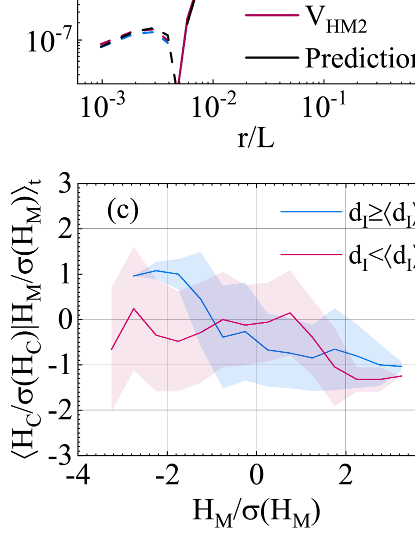
Figure 5: Evidence of solar wind data. (a) Numerical verifications of $V_{HM1}$ and $V_{HM2}$. Solid lines: positive values; dashed lines: negative values. (b) Example of the linear scaling in solar wind. (c) Conditional average of the cross helicity versus the magnetic helicity. (d) The normalized cascade rates versus the normalized cross helicity.

FIG. 5 (a) verifies the vKH relations using the results of H40, where black curves are predictions in Eq. (4) with $\varepsilon_{HMI}=4.4\times 10^{-4}$ and $\varepsilon_{HMF}=1.0\times 10^{-4}$. The equivalent cascade rates are estimated through the fluxes over corresponding wavenumber ranges in SM (sup, ). As shown, $V_{HM1}$ and $V_{HM2}$ are almost the same. At the scale $r/L<0.2$, they both fit well with the predictions. In contrast, at the scale $r/L\gtrapprox 0.2$, the results deviate from the prediction, attributed to the simple inertial range assumption (Xie and Bühler, 2019). To further verify the vKH relations, 8 minute averaged time series for solar wind during day 209/1993 - day 253/1994, day 212/1995 - day 224/1996 and day 20/2006 - day 23/2007 of the Ulysses spacecraft are evaluated (Balogh et al., 1995; Smith et al., 1995). The three periods are very close to solar activity minima, and the heliocentric distance ranges from 2.5 to 4.5 AU (Marino et al., 2012). Using the Taylor hypothesis (Taylor, 1938), the vKH relation for magnetic helicity $V_{HM}(\tau)=\left\langle-V_{L}\tau\delta(v_{3}b_{2}-v_{2}b_{3})\delta b_{L}/2-d_{I}\delta(b_{L}b_{i})b_{i}^{\ast}\right\rangle_{t}=-\varepsilon_{HM}V_{L}\tau/3$, where $V_{L}$ is the averaged longitudinal velocity, $\tau$ is the time lag, $\left\langle\cdot\right\rangle_{t}$ represents the time average, $b_{i}$ is normalized by $(4\pi\rho)^{-1/2}$, and $\rho$ is the mass density. FIG. 5 (b) gives one example of linear scaling related to $V_{HM1}(\tau)$, using data of days 49-59 in 2006. As shown, $V_{HM1}(\tau)$ is linear among nearly two decades with $\varepsilon_{HM}=-8.9\times 10^{11}\textrm{J}\cdot\textrm{m/(kg}\cdot\textrm{s})$.

Based on vKH relations, the turbulent space plasma can be recognized, and the magnetic helicity dissipation rates can be measured. Limited by the data resolution, the Hall effects on the inverse cascades cannot be directly recognized. Therefore, we decompose the numerical finding into two parts: the cross helicity generation, and the cascade efficiency suppression by cross helicity. Notably, in the actual solar wind, the cross helicity could also originate from other effects. In FIG. 5 (c), the conditional average of the cross helicity ($H_{C}$) versus the magnetic helicity ($H_{M}$) is evaluated. Averaged over every 11 days, $H_{M}$ and $H_{C}$ at the timescale $\delta t\in(8\,\textrm{min},4\,\textrm{h})$ are obtained by the Fourier expansion (Brandenburg et al., 2011; Matthaeus and Goldstein, 1982). The results at other timescales are consistent with our main findings and are given in SM (sup, ). As shown in FIG. 5 (c), when the Hall effects are relatively important ($d_{I}\geq\left\langle d_{I}\right\rangle_{t}$), $H_{C}$ is strongly anticorrelated with $H_{M}$. In contrast, when $d_{I}<\left\langle d_{I}\right\rangle_{t}$, $H_{C}$ is relatively independent with $H_{M}$, except for the extreme event ($H_{M}/\sigma(H_{M})\gtrapprox 2$). Even if the data with an 8-min resolution is insufficient to resolve the Hall effects, the remarkable anticorrelation between $H_{C}$ and $H_{M}$ when $d_{I}\geq\left\langle d_{I}\right\rangle_{t}$ imply that Hall effects and magnetic helicity could induce non-zero cross helicity. FIG. 5 (d) shows the conditional average of the normalized cascade rates $\varGamma_{HM}=|\varepsilon_{HM}|/[|\delta{\bf v}||\delta{\bf b}|^{2}V_{L}\tau]$ versus the normalized cross helicity $|\cos\theta_{t}|=|\delta{\bf v}\cdot\delta{\bf b}|/|\delta{\bf v}||\delta{\bf b}|$, where the distance ${r}$ is given by the middle scales with linear scaling. As shown, the normalized cascade rates are anticorrelated with $|\cos\theta_{t}|$, consistent with our numerical findings.

In this letter, we perform six DNSs with grid points up to $2048^{3}$ to investigate Hall effects on helical MHD turbulence. We find that Hall effects could induce strong cross helicity by geometric alignments, which then strongly reduces inverse cascade efficiencies and leads to the accumulation of magnetic energy and helicity at large scales. The process is associated with the breaking of current sheets by filaments along magnetic fields. Then, we derive two vKH relations and verify them using the numerical and Ulysses data. The numerical findings about the cross helicity generation and the cascade efficiency suppression are then separately confirmed by the solar wind results. In the heliosphere, partial extreme solar wind events are generated by the eruption of the solar corona, where magnetic helicity and Hall effects both matter. Generally, one may believe that Hall effects are negligible in large-scale solar wind (Marino and Sorriso-Valvo, 2023). However, this letter gives a possible mechanism in solar wind turbulence that Hall effects at small scales could strongly affect large-scale magnetic fields through cross helicity.