Improved scalar auxiliary variable schemes for original energy stability of gradient flows

Abstract.

Scalar auxiliary variable (SAV) methods are a class of linear schemes for solving gradient flows that are known for the stability of a ‘modified’ energy. In this paper, we propose an improved SAV (iSAV) scheme that not only retains the complete linearity but also ensures rigorously the stability of the original energy. The convergence and optimal error bound are rigorously established for the iSAV scheme and discussions are made for its high-order extension. Extensive numerical experiments are done to validate the convergence, robustness and energy stability of iSAV, and some comparisons are made.

Keywords. gradient flows, improved scalar auxiliary variable scheme, original energy stability, Allen–Cahn and Cahn–Hilliard equations, convergence

AMS(2010) subject classifications. 65M12, 35K20, 35K35, 35K55, 65Z05

1. Introduction

The gradient flow that consists of a driving free energy and a dissipative mechanism, widely occurs in mathematical modelling of natural science and engineering, e.g., the interface dynamics, crystallization, thin films, liquid crystals et al. [1, 19, 29, 13, 17, 18, 25, 24]. In this paper, we consider a free energy functional $\mathcal{E}[\phi]$ defined for functions on a bounded spatial domain $\Omega\subset{\mathbb{R}}^{d}$ ($d=1,2,3$) and the general gradient flow of the following form:

$$\frac{\partial\phi}{\partial t}=-\mathcal{G}\mu,\quad\mu=\delta\mathcal{E}/\delta\phi,$$ (1.1)

where $\mathcal{G}$ is a nonnegative symmetric linear operator that determines the dissipative mechanism. The common dissipative mechanisms include the $L^{2}$ gradient flow (i.e., $\mathcal{G}=I$) and the $H^{-\alpha}$ gradient flow (i.e., $\mathcal{G}=(-\Delta)^{\alpha}$ with $0<\alpha\leq 1$). We supplement (1.1) with boundary conditions satisfying the integration-by-parts, resulting in the elimination of all boundary terms for simplicity. Typically, periodic boundary conditions, homogeneous Neumann and Dirichlet boundary conditions are all applicable. With $\langle\phi,\psi\rangle:=\int_{\Omega}{\phi\psi}\,{\rm d}{\bf x}$ denoting the $L^{2}$ inner product, the energy dissipation law of (1.1) reads

$$\frac{{\rm d}\mathcal{E}[\phi]}{{\rm d}t}=\left\langle\frac{\delta\mathcal{E}}{\delta\phi},\frac{\partial\phi}{\partial t}\right\rangle=-\langle\mu,\mathcal{G}\mu\rangle\leq 0.$$

For accurately and efficiently solving (1.1), extensive numerical methods have been proposed. The classical approaches are the fully implicit schemes, e.g., the backward Euler, Crank-Nicolson and the convex splitting [35, 7, 42, 32, 14, 15]. They can provide the decrease of the energy at discrete time level, but nonlinear solvers are needed at each time step, which is often costly. Concerning strong stability issues of explicit schemes, the semi-implicit schemes which need only linear solvers at each time step, have become popular, particularly when some tailored stabilization techniques [35, 38, 37, 5, 36, 26] can be proposed to overcome the stability constraint from explicitly treating the nonlinearity. Another major class of methods are the exponential time difference methods [12, 23, 41], which can be designed to meet the energy stability and/or the maximum bound principle. For more complete and detailed reviews, we refer to [12, 11, 34] and the references therein.

Among the semi-implicit methods, the modern approach is to introduce some auxiliary variable to the problem which induces the state-of-art: invariant energy quadratization (IEQ) methods [6, 44, 45, 46, 47, 48] and the scalar auxiliary variable (SAV) methods [8, 34, 21, 33]. Both IEQ and SAV provide framework that enables to construct linear and high-order schemes, and their main advantage is to provide the unconditional stability of an approximated/modified energy. Compared to IEQ, SAV is more explicit in the sense that the matrix for inversion at each time step is a constant, whereas that of IEQ is varying in the time iteration. We shall focus on the SAV method in this work.

Ever since the born of the original SAV [34], the improvements on it have been started. For instance, [21, 9, 49, 28, 20, 39] considered the elimination of restrictions on the lower bound of the free energy, or the positivity-preservation of the auxiliary variable. Among all possible directions of improvements, the main target is for the stability of the original energy, because the modified energy dissipation law in SAV (and IEQ) cannot guarantee the dissipation of the original model in theory and counterexamples can be observed in practical computing. To this aim, effective stabilization terms have been designed and added to SAV methods [50, 51, 3] (also stabilized-IEQ [43]) to enhance the practical performance. [22, 27] proposed relaxation techniques to improve the correlation between the modified energy and the original energy. Cheng et al. [8] proposed to use the Lagrange multiplier for the original energy-stability, while the price is to solve a nonlinear algebraic equation per time level.

In this paper, we are going to propose an improved SAV (iSAV) scheme for solving (1.1) particularly aiming for the original energy stability. It is linear with only the constant-coefficient matrix for inversion, and more importantly, it provides the dissipation of the original energy at discrete level as (see Theorem 2.1):

$$\frac{1}{\tau}\left(\mathcal{E}[\phi^{n+1}]-\mathcal{E}[\phi^{n}]\right)\leq-\left\langle\mu^{n+1},\mathcal{G}\mu^{n+1}\right\rangle,\quad n\geq 0.$$

The key ideas consist of: 1) replacing the numerical value of the scalar variable $r^{n}$ in the backward Euler discretization by the original functional $r[\phi^{n}]$ of the scalar variable; 2) introducing a stabilization term. They are inspired from the work for the IEQ method [4] but which is restricted to the double-well potential case. The proposed iSAV method here works for general potential functions bounded from below, and we shall rigorously establish its first-order error bound (see Theorem 3.1). A possible second-order extension will also be discussed. The theoretical energy-stability and accuracy will be supported by numerical experiments. Comparisons with the original SAV will be made to illustrate the improvement.

The rest of this paper is organized as follows. In Section 2, we present the iSAV schemes and establish the original energy stability result. In Section 3, we provide an error estimate for the proposed scheme. The numerical results and comparisons are given in Section 4, and some conclusions are drawn in Section 5. The following are some notations that will be frequently used in the paper. The standard $L^{p}=L^{p}(\Omega)$ space and the Sobolev space $H^{s}=H^{s}(\Omega)$ with $s>0$ are utilized. $L^{p}(0,T;V)$ denotes the $L^{p}$ space on the time interval $(0,T)$ with values in the functional space $V$. The norm of the space $V$ is denoted by $\|\cdot\|_{V}$ and specifically, the $L^{2}$ norm is denoted without a subscript. For a nonnegative symmetric linear operator, such as $\mathcal{G}$, we denote $\left\langle\phi,\mathcal{G}\phi\right\rangle^{\frac{1}{2}}=\|\mathcal{G}^{\frac{1}{2}}\phi\|$ for short. The notation $a=\mathcal{O}(b)$ or $a\lesssim b$ means that there exists a constant $C>0$, whose value may vary from line to line, but is independent of the numerical discrete parameters (e.g., the step size $\tau$ or the time level $n$), such that $\left|a\right|\leq Cb$.

2. Improved SAV scheme

In this section, we shall present the main numerical schemes for solving the gradient flows. To be precise, let us clearly state our setup of the problem. We focus on the following form of free energy:

$$\mathcal{E}[\phi]=\frac{1}{2}\left\|\mathcal{L}^{\frac{1}{2}}\phi\right\|^{2}+\int_{\Omega}{F(\phi)}\,{\rm d}{\bf x},\quad\Omega\subset{\mathbb{R}}^{d},\ d=1,2,3,$$

and its gradient flow (1.1) then reads as

$$\frac{\partial\phi}{\partial t}=-\mathcal{G}\mu,\quad t>0,\ \mathbf{x}\in\Omega,$$ (2.1a)

$$\mu=\mathcal{L}\phi+f(\phi),$$ (2.1b)

where $\mathcal{L}$ is a symmetric nonnegative linear operator that is independent of $\phi=\phi(\mathbf{x},t)$, and $F(\phi)$ denotes the bulk part of the free energy density which is usually nonlinear (e.g., a double well form $F(\phi)=\frac{1}{4\varepsilon^{2}}(\phi^{2}-1)^{2}$) with $f(\phi):=F^{\prime}(\phi)$. From the application point of view [34], $\int_{\Omega}{F(\phi)}\,{\rm d}{\bf x}$ is often bounded from below. So without loss of generality, we assume that

$$\int_{\Omega}{F(\phi)}\,{\rm d}{\bf x}\geq C_{0}>0,$$

otherwise we can add a constant to $F(\phi)$ without changing the gradient flow (2.1). The boundary of the bounded domain $\Omega$ is set to be periodic for (2.1) for simplicity.

2.1. The SAV framework

We begin with a brief review of the SAV method introduced in [34]. The first key step for the SAV approach is to introduce a scalar variable:

$$\mathcal{F}[\phi]:=\int_{\Omega}F(\phi)\,d\mathbf{x},\quad r(t):=r[\phi]:=\sqrt{\mathcal{F}[\phi]},$$

and then (2.1) can be rewritten as a system:

$$\frac{\partial\phi}{\partial t}=-\mathcal{G}\mu,\quad t>0,\ \mathbf{x}\in\Omega,$$ (2.2a)

$$\,\mu=\mathcal{L}\phi+\frac{r}{\sqrt{\mathcal{F}[\phi]}}f(\phi),$$ (2.2b)

$$\frac{{\rm d}r}{{\rm d}t}=\frac{1}{2\sqrt{\mathcal{F}[\phi]}}\int_{\Omega}f(\phi)\frac{\partial\phi}{\partial t}\,{\rm d}{\bf x},\quad t>0.$$ (2.2c)

Taking the $L^{2}$ inner products of (2.2a) and (2.2b) with $\mu$ and $\frac{\partial\phi}{\partial t}$, respectively, multiplying (2.2c) by $2r$, and then by adding them together, the energy dissipative law of the gradient flow (2.1) can be seen

$$\frac{{\rm d}\mathcal{E}[\phi]}{{\rm d}t}=\frac{{\rm d}}{{\rm d}t}\left(\frac{1}{2}\left\|\mathcal{L}^{\frac{1}{2}}\phi\right\|^{2}+r^{2}\right)=-\|\mathcal{G}^{\frac{1}{2}}\mu\|^{2},\quad t>0.$$ (2.3)

Numerical discretizations can then be considered for (2.2). By the backward Euler type of finite difference discretization with explicit treatment of the nonlinear terms in (2.2), a first-order SAV scheme (SAV-BE) was constructed in [34]: for $n\geq 0$,

$$\frac{1}{\tau}(\phi^{n+1}-\phi^{n})=-\mathcal{G}\mu^{n+1},$$ (2.4a)

$$\mu^{n+1}=\mathcal{L}\phi^{n+1}+\frac{r^{n+1}}{\sqrt{\mathcal{F}[\phi^{n}]}}f(\phi^{n}),$$ (2.4b)

$$r^{n+1}-r^{n}=\frac{1}{2\sqrt{\mathcal{F}[\phi^{n}]}}\int_{\Omega}f(\phi^{n})(\phi^{n+1}-\phi^{n})\,{\rm d}{\bf x}.$$ (2.4c)

The first advantage of the scheme is its linearity, where $\phi^{n+1}$ can be obtained from (2.4) by solving two linear systems. We refer the readers to [34] for the detailed update procedure. Moreover, by taking the $L^{2}$ inner products of (2.4a) and (2.4b) with $\mu^{n+1}$ and $\frac{1}{\tau}(\phi^{n+1}-\phi^{n})$, respectively, multiplying (2.4c) by $2\frac{r^{n+1}}{\tau}$, and then adding them together, one can obtain a discrete energy dissipative law for SAV-BE (2.4) as

$$\frac{1}{\tau}\left(E^{n+1}-E^{n}\right)\leq-\left\|\mathcal{G}^{\frac{1}{2}}\mu^{n+1}\right\|^{2},\quad E^{n}:=\frac{1}{2}\left\|\mathcal{L}^{\frac{1}{2}}\phi^{n}\right\|^{2}+\left(r^{n}\right)^{2},\quad n\geq 0,$$ (2.5)

which gives the ‘energy’ stability. However, $r^{n}\neq r[\phi^{n}]$ for $n\geq 1$, and this may lead to oscillations in the evolution of the original energy $\mathcal{E}[\phi^{n}]$ of the gradient flow and the occurrence of numerical instability.

In fact, for the behaviour of the original energy in the SAV-BE scheme (2.4), we can give the following formal estimate (derivation given in Appendix A):

$$\frac{1}{\tau}\left(\mathcal{E}[\phi^{n+1}]-\mathcal{E}[\phi^{n}]\right)\leq-\|\mathcal{G}^{\frac{1}{2}}\mu^{n+1}\|^{2}+\mathcal{O}(\tau),\quad n\geq 0,$$ (2.6)

which indicates that the original energy stability needs the time step to be small enough. This can get worse when the nonlinearity is stiff, e.g., $F(\phi)=\frac{1}{\varepsilon^{2}}(\phi^{2}-1)^{2}$ for some parameter $0<\varepsilon<1$, where (2.6) will at least deteriorate to:

$$\frac{1}{\tau}\left(\mathcal{E}[\phi^{n+1}]-\mathcal{E}[\phi^{n}]\right)\leq-\|\mathcal{G}^{\frac{1}{2}}\mu^{n+1}\|^{2}+\mathcal{O}(\tau/\varepsilon^{2}),\quad n\geq 0.$$

So if $\varepsilon\ll 1$ while $\tau$ is not sufficiently small, the original energy of the SAV schemes could easily be unstable and the oscillations could get wilder as $\varepsilon$ reduces. Higher-order SAV schemes [34, 33] exhibit such problem as well. Suitable stabilization techniques need to be considered for SAV [30] for the better practical performance.

2.2. Improved SAV scheme

Concerning the pity of SAV schemes, we aim to suggest a patch for it. We begin with the work on the first-order scheme. Reviewing the SAV-BE scheme, $r^{n}$ is used to update $r^{n+1}$ in (2.4c), which indeed leads to a growing disparity between the values of $r^{n}$ and $r[\phi^{n}]$. Therefore, we consider to replace $r^{n}$ by $r[\phi^{n}]$ in (2.4c) and add a stabilization term in (2.4b). This results in the following scheme that we name as the first-order improved SAV-BE scheme (iSAV-BE): for $n\geq 0$,

$$\frac{1}{\tau}(\phi^{n+1}-\phi^{n})=-\mathcal{G}\mu^{n+1},$$ (2.7a)

$$\mu^{n+1}=\mathcal{L}\phi^{n+1}+\frac{\tilde{r}^{n+1}}{\sqrt{\mathcal{F}[\phi^{n}]}}f(\phi^{n})+S(\phi^{n+1}-\phi^{n}),$$ (2.7b)

$$\tilde{r}^{n+1}-r[\phi^{n}]=\frac{1}{2\sqrt{\mathcal{F}[\phi^{n}]}}\int_{\Omega}{f(\phi^{n})(\phi^{n+1}-\phi^{n})}\,{\rm d}{\bf x},$$ (2.7c)

where $S\geq 0$ is a stabilizing parameter to be determined.

For the proposed iSAV-BE (2.7), firstly, it is still a linear scheme and $\phi^{n+1}$ can be obtained efficiently as follows. Note that the two auxiliary variables $\mu^{n+1}$ and $\tilde{r}^{n+1}$ can be eliminated by combining (2.7a)$\sim$(2.7c), and we can find

$$\frac{1}{\tau}\left(\phi^{n+1}-\phi^{n}\right)= -\mathcal{G}\mathcal{L}\phi^{n+1}-\frac{\mathcal{G}f(\phi^{n})}{\sqrt{\mathcal{F}[\phi^{n}]}}\left(r[\phi^{n}]+\frac{1}{2}\left\langle\frac{f(\phi^{n})}{\sqrt{\mathcal{F}[\phi^{n}]}},\phi^{n+1}-\phi^{n}\right\rangle\right)-S\mathcal{G}(\phi^{n+1}-\phi^{n}).$$

Denoting $b^{n}:=f(\phi^{n})/\sqrt{\mathcal{F}[\phi^{n}]}$, the above equation can be rewritten as

$$\left[I+\tau\mathcal{G}\left(\mathcal{L}+S\right)\right]\phi^{n+1}+\frac{\tau}{2}\left\langle b^{n},\phi^{n+1}\right\rangle\mathcal{G}b^{n}$$

$$= \left(I+\tau S\mathcal{G}\right)\phi^{n}-\tau\left(r[\phi^{n}]-\frac{1}{2}\left\langle b^{n},\phi^{n}\right\rangle\right)\mathcal{G}b^{n}=:g^{n}.$$ (2.8)

Since $\mathcal{G}$ and $\mathcal{L}$ are nonnegative operators, the operator $I+\tau\mathcal{G}(\mathcal{L}+S)$ is invertible and we denote

$$\mathcal{A}^{-1}:=\left[I+\tau\mathcal{G}(\mathcal{L}+S)\right]^{-1}.$$

Then, by multiplying (2.8) on both sides with $\mathcal{A}^{-1}$ and taking the $L^{2}$ inner product with $b^{n}$, we can obtain

$$\langle b^{n},\phi^{n+1}\rangle+\frac{\tau}{2}\langle b^{n},\phi^{n+1}\rangle\langle b^{n},\mathcal{A}^{-1}\mathcal{G}b^{n}\rangle=\langle b^{n},\mathcal{A}^{-1}g^{n}\rangle,\quad n\geq 0.$$ (2.9)

Based on the above two equations, we can compute $\phi^{n+1}$ (semi-discretized numerical solution) from (2.7) through the following steps: for $n\geq 0$,

1. compute $\langle b^{n},\mathcal{A}^{-1}\mathcal{G}b^{n}\rangle$ and $\langle b^{n},\mathcal{A}^{-1}g^{n}\rangle$, where $\mathcal{A}^{-1}\mathcal{G}b^{n}$ and $\mathcal{A}^{-1}g^{n}$ can be calculated by solving two linear systems with constant coefficients;

2. compute $\langle b^{n},\phi^{n+1}\rangle$ from (2.9) as

   $$\langle b^{n},\phi^{n+1}\rangle=\langle b^{n},\mathcal{A}^{-1}g^{n}\rangle/\left(1+\frac{\tau}{2}\langle b^{n},\mathcal{A}^{-1}\mathcal{G}b^{n}\rangle\right),$$

   where $1+\frac{\tau}{2}\langle b^{n},\mathcal{A}^{-1}\mathcal{G}b^{n}\rangle\geq 1$ clearly;

3. obtain $\phi^{n+1}$ from (2.8) as

   $$\phi^{n+1}=-\frac{\tau}{2}\langle b^{n},\phi^{n+1}\rangle\mathcal{A}^{-1}\mathcal{G}b^{n}+\mathcal{A}^{-1}g^{n}.$$

The invertibility of $\mathcal{A}$ also indicates the uniqueness of the numerical solution from the iSAV-BE scheme (2.7). We shall rigorously prove in the next section that it is a first order accurate method in time. For the practical implementation, the spatial discretizations can be done by the Fourier pseudo-spectral method [31] under the periodic setup, and the involved linear systems in above procedure (i)&(iii) are then automatically diagonalized by the fast Fourier transform. Thus, the whole scheme can work efficiently in a matrix-free way. For other spatial discretizations in general, since $\mathcal{A}^{-1}$ is constant in the temporal iteration, it can be pre-computed and stored once for all.

Next, we will give the main improvement from the iSAV-BE scheme that is the stability of the original energy of the gradient flow.

Theorem 2.1 (Original energy stability).

Suppose (2.1) is solved by the iSAV-BE scheme (2.7) till some $0<T<\infty$, and we choose the stabilizing parameter $S$ to satisfy

$$S\geq S_{0}:=\frac{1}{2}\max_{0\leq n\leq T/\tau-1}\;\max_{\mathbf{x}\in\Omega,\,\rho\in(0,1)}\left\{f^{\prime}\left(\left(1-\rho\right)\phi^{n}+\rho\phi^{n+1}\right)\right\}.$$ (2.10)

Then, the iSAV-BE scheme (2.7) has the following discrete energy disspative law,

$$\frac{1}{\tau}\left(\mathcal{E}[\phi^{n+1}]-\mathcal{E}[\phi^{n}]\right)\leq-\|\mathcal{G}^{\frac{1}{2}}\mu^{n+1}\|^{2},\quad 0\leq n\leq T/\tau-1.$$ (2.11)

After Corollary 3.2, we will further show that $S_{0}$ can be a fixed finite number, and so an $S\in[S_{0},\infty)$ can be chosen.

Proof.

By taking the $L^{2}$ inner products of (2.7a) and (2.7b) with $\mu^{n+1}$ and $(\phi^{n+1}-\phi^{n})/\tau$, respectively, and multiplying (2.7c) by $\frac{2\tilde{r}^{n+1}}{\tau}$, we can obtain the following equations:

$$\frac{1}{\tau}\left\langle\phi^{n+1}-\phi^{n},\mu^{n+1}\right\rangle=-\left\|\mathcal{G}^{\frac{1}{2}}\mu^{n+1}\right\|^{2},$$ (2.12a)

$$\frac{1}{\tau}\left\langle\mu^{n+1},\phi^{n+1}-\phi^{n}\right\rangle=\frac{1}{\tau}\left\langle\mathcal{L}\phi^{n+1},\phi^{n+1}-\phi^{n}\right\rangle+\frac{\tilde{r}^{n+1}}{\tau}\left\langle\frac{f(\phi^{n})}{\sqrt{\mathcal{F}[\phi^{n}]}},\phi^{n+1}-\phi^{n}\right\rangle+\frac{S}{\tau}\left\|\phi^{n+1}-\phi^{n}\right\|^{2}$$

$$\hskip 89.34163pt=\frac{1}{2\tau}\left(\left\|\mathcal{L}^{\frac{1}{2}}\phi^{n+1}\right\|^{2}-\left\|\mathcal{L}^{\frac{1}{2}}\phi^{n}\right\|^{2}+\left\|\mathcal{L}^{\frac{1}{2}}(\phi^{n+1}-\phi^{n})\right\|^{2}\right)+\frac{S}{\tau}\left\|\phi^{n+1}-\phi^{n}\right\|^{2}$$

$$\hskip 105.2751pt+\frac{\tilde{r}^{n+1}}{\tau}\left\langle\frac{f(\phi^{n})}{\sqrt{\mathcal{F}[\phi^{n}]}},\phi^{n+1}-\phi^{n}\right\rangle,$$ (2.12b)

$$\frac{1}{\tau}\left[\left(\tilde{r}^{n+1}\right)^{2}-\left(r[\phi^{n}]\right)^{2}+\left(\tilde{r}^{n+1}-r[\phi^{n}]\right)^{2}\right]=\frac{\tilde{r}^{n+1}}{\tau}\left\langle\frac{f(\phi^{n})}{\sqrt{\mathcal{F}[\phi^{n}]}},\phi^{n+1}-\phi^{n}\right\rangle.$$ (2.12c)

Plugging (2.12a) into the left hand side of (2.12b) and plugging (2.12c) into the right hand side of (2.12b), we get

$$-\frac{1}{\tau}\left[\left(\tilde{r}^{n+1}\right)^{2}-\left(r[\phi^{n}]\right)^{2}+\left(\tilde{r}^{n+1}-r[\phi^{n}]\right)^{2}\right]$$

$$= \left\|\mathcal{G}^{\frac{1}{2}}\mu^{n+1}\right\|^{2}+\frac{1}{2\tau}\left(\left\|\mathcal{L}^{\frac{1}{2}}\phi^{n+1}\right\|^{2}-\left\|\mathcal{L}^{\frac{1}{2}}\phi^{n}\right\|^{2}+\left\|\mathcal{L}^{\frac{1}{2}}(\phi^{n+1}-\phi^{n})\right\|^{2}\right)+\frac{S}{\tau}\left\|\phi^{n+1}-\phi^{n}\right\|^{2}.$$

Plugging (2.7c) into the left hand side of the above, we can find

$$\frac{1}{\tau}\left(\tilde{E}^{n+1}-\mathcal{E}[\phi^{n}]\right)=-\left\|\mathcal{G}^{\frac{1}{2}}\mu^{n+1}\right\|^{2}-\frac{S}{\tau}\left\|\phi^{n+1}-\phi^{n}\right\|^{2}-\mathcal{N}_{1}^{n},$$ (2.13)

where $\tilde{E}^{n+1}$ and $\mathcal{N}_{1}^{n}$ denote

$$\tilde{E}^{n+1}=\frac{1}{2}\left\|\mathcal{L}^{\frac{1}{2}}\phi^{n+1}\right\|^{2}+\left(\tilde{r}^{n+1}\right)^{2},$$

$$\mathcal{N}_{1}^{n}=\frac{1}{2\tau}\left\|\mathcal{L}^{\frac{1}{2}}\left(\phi^{n+1}-\phi^{n}\right)\right\|^{2}+\frac{1}{4\tau}\frac{1}{\mathcal{F}[\phi^{n}]}\left(\int_{\Omega}{f(\phi^{n})\left(\phi^{n+1}-\phi^{n}\right)}\,{\rm d}{\bf x}\right)^{2}.$$

Next, we proceed to derive the difference between $\tilde{E}^{n+1}$ and $\mathcal{E}[\phi^{n}]$. Note that by the Taylor expansion,

$$\mathcal{F}\left[\phi^{n}+\rho\left(\phi^{n+1}-\phi^{n}\right)\right]$$

$$= \mathcal{F}\left[{\phi^{n}}\right]+\frac{{\rm d}}{{\rm d}\rho}\mathcal{F}\left[\phi^{n}+\rho\left(\phi^{n+1}-\phi^{n}\right)\right]\Big{|}_{\rho=0}\cdot\rho+\frac{{\rm d}^{2}}{{\rm d}\rho^{2}}\mathcal{F}\left[\phi^{n}+\rho\left(\phi^{n+1}-\phi^{n}\right)\right]\Big{|}_{\rho=\rho_{0}}\cdot\frac{\rho^{2}}{2}$$

$$= \mathcal{F}\left[\phi^{n}\right]+\rho\int_{\Omega}{f\left(\phi^{n}\right)\left(\phi^{n+1}-\phi^{n}\right)}\,{\rm d}{\bf x}+\frac{\rho^{2}}{2}\int_{\Omega}{f^{\prime}\left((1-\rho_{0})\phi^{n}+\rho_{0}\phi^{n+1}\right)\left(\phi^{n+1}-\phi^{n}\right)^{2}}\,{\rm d}{\bf x},$$

for some $\rho_{0}\in(0,\rho)$, and so with $\rho=1$ we have

$$\left(r[\phi^{n+1}]\right)^{2}-\left(r[\phi^{n}]\right)^{2} =\mathcal{F}[\phi^{n+1}]-\mathcal{F}[\phi^{n}]$$

$$=\int_{\Omega}{f(\phi^{n})\left(\phi^{n+1}-\phi^{n}\right)}\,{\rm d}{\bf x}+\frac{1}{2}\int_{\Omega}{f^{\prime}\left((1-\rho_{0})\phi^{n}+\rho_{0}\phi^{n+1}\right)(\phi^{n+1}-\phi^{n})^{2}}\,{\rm d}{\bf x}.$$ (2.14)

Additionally from (2.7c): $\tilde{r}^{n+1}=r[\phi^{n}]+\frac{1}{2\sqrt{\mathcal{F}[\phi^{n}]}}\int_{\Omega}{f(\phi^{n})(\phi^{n+1}-\phi^{n})}\,{\rm d}{\bf x}$, then by taking the square on both sides, we obtain

$$\left(\tilde{r}^{n+1}\right)^{2}-\left(r[\phi^{n}]\right)^{2}=\int_{\Omega}{f(\phi^{n})\left(\phi^{n+1}-\phi^{n}\right)}\,{\rm d}{\bf x}+\frac{1}{4\mathcal{F}[\phi^{n}]}\left(\int_{\Omega}{f(\phi^{n})\left(\phi^{n+1}-\phi^{n}\right)}\,{\rm d}{\bf x}\right)^{2}.$$ (2.15)

Subtracting (2.15) from (2.14), we have

$$\left(r[\phi^{n+1}]\right)^{2}-\left(\tilde{r}^{n+1}\right)^{2}= \frac{1}{2}\int_{\Omega}{f^{\prime}\left((1-\rho_{0})\phi^{n}+\rho_{0}\phi^{n+1}\right)(\phi^{n+1}-\phi^{n})^{2}}\,{\rm d}{\bf x}$$

$$-\frac{1}{4\mathcal{F}[\phi^{n}]}\left(\int_{\Omega}{f(\phi^{n})\left(\phi^{n+1}-\phi^{n}\right)}\,{\rm d}{\bf x}\right)^{2}.$$ (2.16)

Then by (2.13),

$$\frac{1}{\tau}\left(\mathcal{E}[\phi^{n+1}]-\mathcal{E}[\phi^{n}]\right)= \frac{1}{\tau}\left(\tilde{E}^{n+1}-\mathcal{E}[\phi^{n}]\right)+\frac{1}{\tau}\left(\mathcal{E}[\phi^{n+1}]-\tilde{E}^{n+1}\right)$$

$$= -\left\|\mathcal{G}^{\frac{1}{2}}\mu^{n+1}\right\|^{2}-\frac{S}{\tau}\left\|\phi^{n+1}-\phi^{n}\right\|^{2}-\mathcal{N}_{1}^{n}+\frac{1}{\tau}\left(\mathcal{E}[\phi^{n+1}]-\frac{1}{2}\left\|\mathcal{L}^{\frac{1}{2}}\phi^{n+1}\right\|^{2}-\left(\tilde{r}^{n+1}\right)^{2}\right),$$

and by plugging (2.16) into the above, we get

$$\frac{1}{\tau}\left(\mathcal{E}[\phi^{n+1}]-\mathcal{E}[\phi^{n}]\right)= \frac{1}{2\tau}\int_{\Omega}{f^{\prime}\left((1-\rho_{0})\phi^{n}+\rho_{0}\phi^{n+1}\right)(\phi^{n+1}-\phi^{n})^{2}}\,{\rm d}{\bf x}-\frac{S}{\tau}\left\|\phi^{n+1}-\phi^{n}\right\|^{2}$$

$$-\left\|\mathcal{G}^{\frac{1}{2}}\mu^{n+1}\right\|^{2}-\mathcal{N}_{2}^{n},$$

with

$$\mathcal{N}_{2}^{n}=\frac{1}{2\tau}\left\|\mathcal{L}^{\frac{1}{2}}\left(\phi^{n+1}-\phi^{n}\right)\right\|^{2}+\frac{1}{2\tau}\frac{1}{\mathcal{F}[\phi^{n}]}\left(\int_{\Omega}{f(\phi^{n})\left(\phi^{n+1}-\phi^{n}\right)}\,{\rm d}{\bf x}\right)^{2}\geq 0.$$

With the condition on the stabilizing parameter (2.10), we can immediately conclude the original energy dissipative law (2.11). ∎

Remark 1.

The stabilizing term $S(\phi^{n+1}-\phi^{n})$ ensures rigorous stability in the dissipation of original energy, and this term is of $\mathcal{O}(\tau)$. Thus, the inclusion of it in the scheme does not affect the overall convergence order.

Remark 2.

Assuming that $\phi^{n},f(\phi^{n}),f^{\prime}(\phi^{n})\;(n=0,1,\cdots)$ and $\phi_{t}$ are bounded, we can formally see that $r[\phi^{n+1}]-\tilde{r}^{n+1}=\mathcal{O}(\tau^{2})$ from (2.16) for iSAV-BE scheme. On the other hand, for the SAV-BE scheme (2.4), we have

$$r[\phi^{n+1}]-r^{n+1}=r[\phi^{n}]-r^{n}+\mathcal{O}(\tau^{2}),$$

which is derived in Appendix A. That means after the accumulation in the temporal iterations, the SAV-BE scheme in general offers only $r[\phi^{n+1}]-r^{n+1}=\mathcal{O}(\tau)$. This will be shown numerically later.

Remark 3.

In practice, the SAV schemes will need to use some stabilization strategy. Taking the SAV-BE (2.4) scheme as an example, a stabilization term is often extracted from $f(\phi^{n})$ and (2.4b) would be modified as

$$\mu^{n+1}=S\phi^{n+1}+\mathcal{L}\phi^{n+1}+\frac{r^{n+1}}{\sqrt{\mathcal{F}[\phi^{n}]}}\left(f(\phi^{n})-S\phi^{n}\right).$$

Such kind of strategy works well in the literature [34, 30] for numerical simulations, while unfortunately it lacks of rigorous analysis and cannot have the theoretical guarantee for the original energy stability. Moreover, the size of the stabilization parameter for SAV [30] is sometimes unknown in advance. For iSAV, such condition is to some extent more explicitly given in (2.10).

2.3. Possible extension

The SAV schemes can have high-order versions. For instance, a second-order scheme can be obtained by using the backward differentiation formula (SAV-BDF) [34]: for $n\geq 1,$

$$\frac{1}{2\tau}\left(3\phi^{n+1}-4\phi^{n}+\phi^{n-1}\right)=-\mathcal{G}\mu^{n+1},$$ (2.17a)

$$\mu^{n+1}=\mathcal{L}\phi^{n+1}+\frac{r^{n+1}}{\sqrt{\mathcal{F}[\phi_{*}^{n+1}]}}f(\phi_{*}^{n+1}),$$ (2.17b)

$$3r^{n+1}-4r^{n}+r^{n-1}=\frac{1}{2\sqrt{\mathcal{F}[\phi_{*}^{n+1}]}}\int_{\Omega}{f(\phi_{*}^{n+1})\left(3\phi^{n+1}-4\phi^{n}+\phi^{n-1}\right)}\,{\rm d}{\bf x}.$$ (2.17c)

The extension of iSAV to high order is, however, not easy unfortunately and it is still under going. Here we discuss some possibility.

Borrowing the modification used for iSAV-BE, we can introduce similar patch to the above SAV-BDF to write down the following iSAV-BDF scheme:

$$\frac{1}{2\tau}\left(3\phi^{n+1}-4\phi^{n}+\phi^{n-1}\right)=-\mathcal{G}\mu^{n+1},$$ (2.18a)

$$\mu^{n+1}=\mathcal{L}\phi^{n+1}+\frac{\tilde{r}^{n+1}}{\sqrt{\mathcal{F}[\phi_{*}^{n+1}]}}f(\phi_{*}^{n+1})+S(\phi^{n+1}-2\phi^{n}+\phi^{n-1}),$$ (2.18b)

$$3\tilde{r}^{n+1}-4r[\phi^{n}]+r[\phi^{n-1}]=\frac{1}{2\sqrt{\mathcal{F}[\phi_{*}^{n+1}]}}\int_{\Omega}{f(\phi_{*}^{n+1})\left(3\phi^{n+1}-4\phi^{n}+\phi^{n-1}\right)}\,{\rm d}{\bf x},$$ (2.18c)

where $\phi_{*}^{n+1}:=2\phi^{n}-\phi^{n-1}$ is the second-order extrapolation for $\phi^{n+1}$. The iSAV-BDF scheme is still linear for solving. Although by numerical experiments later, we shall show that the iSAV-BDF (2.18) can remarkably improve the stability for the original energy compared to the SAV-BDF (2.17), we are encountering difficulty to rigorously prove its original energy stability. By assuming enough smoothness and boundedness for $f,\phi$ and $\phi^{n}\;(n=0,1,\cdots)$, what we are able to show for the iSAV-BDF scheme (2.18) is

$$\frac{1}{\tau}\left(\mathcal{E}_{2}[\phi^{n+1},\phi^{n}]-\mathcal{E}_{2}[\phi^{n},\phi^{n-1}]\right)\leq-\left\|\mathcal{G}^{\frac{1}{2}}\mu^{n+1}\right\|^{2}+\mathcal{O}(\tau^{2}),$$ (2.19)

where $\mathcal{E}_{2}$ is defined as

$$\mathcal{E}_{2}[\phi^{n},\phi^{n-1}]:= \frac{1}{4}\left(\left\|\mathcal{L}^{\frac{1}{2}}\phi^{n}\right\|^{2}+\left\|\mathcal{L}^{\frac{1}{2}}\left(2\phi^{n}-\phi^{n-1}\right)\right\|^{2}\right)+\frac{1}{2}\left[\left(r[\phi^{n}]\right)^{2}+\left(2r[\phi^{n}]-r[\phi^{n-1}]\right)^{2}\right]$$

$$+\frac{S}{2}\left\|\phi^{n}-\phi^{n-1}\right\|^{2}.$$

We leave the derivation of (2.19) to Appendix B.

Remark 4.

Similarly as in Remark 2, we can derive the difference between the auxiliary variables $r^{n}$ and $r[\phi^{n}]$ in SAV-BDF and iSAV-BDF as

$$r[\phi^{n}]-\tilde{r}^{n}=\mathcal{O}(\tau^{3}),\quad\text{for iSAV-BDF (\ref{iSAV-BDF scheme})};$$

$$r[\phi^{n}]-r^{n}=\mathcal{O}(\tau^{2}),\quad\text{for SAV-BDF (\ref{SAV-BDF scheme})}.$$

The detailed derivations are omitted here for brevity.

3. Convergence analysis

In this section, we carry out rigorous convergence analysis for the proposed iSAV-BE scheme (2.7). The main convergence theorem is stated in Section 3.1, and the rest of the section is devoted for the proof. In the analysis, a large number of constants $C$ will appear whose value may vary from line to line, and we will use the notation $C(\cdot)$ to indicate its dependence when needed.

3.1. Main convergence result

We restrict the spatial dimension to be no more than three dimensions, i.e., $d\leq 3$, and consider only one typical case of the gradient flow for analysis: the Cahn-Hilliard equation, i.e., $\mathcal{L}=-\Delta$ and $\mathcal{G}=-\Delta$ in (2.1). Assume that $F\in C^{5}(\mathbb{R})$ and $f$ satisfies

$$|f^{\prime}(z)|\leq C\cdot\big{(}|z|^{p}+1\big{)},\quad\ p>0\;\;\ {\rm arbitrary\;\;if}\;\;d=1,2;\quad 0<p<4\;\;{\rm if}\;\;d=3,$$ (3.1a)

$$|f^{\prime\prime}(z)|\leq C\cdot\big{(}|z|^{p^{\prime}}+1\big{)},\quad{p^{\prime}}>0\;\;{\rm arbitrary\;\;if}\;\;d=1,2;\quad 0<{p^{\prime}}<3\;\;{\rm if}\;\;d=3,$$ (3.1b)

and the exact solution $\phi$ of (2.1) up to $0\leq t\leq T$ with some $0<T<\infty$ satisfies [33]:

$$\phi\in L^{\infty}(0,T;H^{2})\cap L^{\infty}(0,T;W^{1,\infty}),\quad\phi_{t}\in L^{\infty}(0,T;H^{-1})\cap L^{2}(0,T;H^{1}),\quad\phi_{tt}\in L^{2}(0,T;H^{-1}).$$ (3.2)

The main convergence result of the iSAV-BE scheme (2.7) is stated as the following theorem.

Theorem 3.1 (Convergence and error bound).

Denote $e_{\phi}^{n}=\phi^{n}-\phi(t_{n})$, $e_{\mu}^{n}=\mu^{n}-\mu(t_{n})$, $\tilde{q}^{n+1}=\tilde{r}^{n+1}-r(t_{n+1})$ with $\phi^{n},\mu^{n},\tilde{r}^{n+1}$ obtained from iSAV-BE (2.7) for any $S\geq 0$, and let both (3.1) and (3.2) hold. Assume that $\phi^{0}\in H^{8}(\Omega)$ and denote $\left\|\phi\right\|_{L^{\infty}(0,T;H^{1})}^{2}=M$, then there exist some constants $\tau_{0},\,C_{1},C_{2}>0$ independent of $n,\tau$ such that for any $0<\tau<\tau_{0}$,

$$\left\|\phi^{n}\right\|_{H^{1}}^{2}\leq M+1,\quad\left\|\phi^{n}\right\|_{L^{\infty}}\leq C_{1},\quad 0\leq n\leq T/\tau,$$ (3.3)

and

$$\frac{1}{2}\left\|e_{\phi}^{n}\right\|_{H^{1}}^{2}+\left|\tilde{q}^{n}\right|^{2}+\frac{\tau}{5}\sum_{k=1}^{n}\left\|\nabla e_{\mu}^{k}\right\|^{2}\leq C_{2}\tau^{2},\quad 0\leq n\leq T/\tau,$$ (3.4)

Here in particular, $C_{1}$ depends on $d,T,M,C_{0}$ and the norms of $\phi^{0},f$ on $\Omega$ but is independent of $S$.

The uniform $L^{\infty}$ bound of the numerical solution in (3.3) can immediately lead to the following result that accomplishes Theorem 2.1.

Corollary 3.2.

Denote $\displaystyle S_{1}=\frac{1}{2}\max_{|\rho|\leq C_{1}}\left\{f^{\prime}\left(\rho\right)\right\}<\infty$. Let the assumptions and conditions in Theorem 3.1 be satisfied, then

$$S_{0}=\frac{1}{2}\max_{0\leq n\leq T/\tau-1}\;\max_{\mathbf{x}\in\Omega,\,\rho\in(0,1)}\left\{f^{\prime}\left(\left(1-\rho\right)\phi^{n}+\rho\phi^{n+1}\right)\right\}\leq S_{1},$$

and so by chosen $S\in[S_{1},\infty)$, the iSAV-BE scheme (2.7) with the original energy-stability (2.11) is well-defined.

The convergence for other gradient flows, e.g., the Allen-Cahn equation ($\mathcal{G}=I,\mathcal{L}=-\Delta$), can be established similarly, and we omit the results here for brevity. We will then prove Theorem 3.1 in the next two subsections.

Remark 5.

Compared to the traditional SAV-BE scheme (see Lemma 2.4 in [33]), the assumption for iSAV-BE in Theorem 3.1 enhances the regularity requirement of $\phi^{0}$ from $H^{4}$ to $H^{8}$. This is only for the technical analysis reason, where an $H^{4}$-bound of the numerical solution is called in the proof (in (3.26)). It should be noted that such condition (even $\phi^{0}\in H^{4}$ for SAV-BE) is not necessary in practical computing. Relaxing the regularity requirement or finding the optimal condition is a future analytical task.

3.2. Prior estimates of numerical solution

To give the proof, we need to first establish some prior estimates for the numerical solution of iSAV-BE and we shall need a tool lemma which we directly quote from [33].

Lemma 3.3 ([33]).

Assume that $\left\|u\right\|_{H^{1}}^{2}\leq M+1$ and (3.1) holds. Then for any $u\in H^{4}$, there exist some $0\leq\sigma\leq 1$ and a constant $C(d,M)>0$ dependent on $d,M$ such that

$$\left\|\Delta f(u)\right\|^{2}\leq C(d,M)\left(1+\left\|\Delta^{2}u\right\|^{2\sigma}\right).$$

Proposition 3.4 ($H^{2}$-boundedness).

Assume that (3.1) holds, $\phi^{0}\in H^{4}(\Omega)$ and $\left\|\phi^{n}\right\|_{H^{1}}^{2}\leq M+1$ for all $0\leq n\leq m$ with some $1\leq m<T/\tau$. Then, there exists a constant $\tau_{1}>0$ independent of $n,m,\tau$ such that for any $0<\tau\leq\tau_{1}$,

$$\left\|\Delta\phi^{n+1}\right\|^{2}+\frac{\tau}{2}\sum_{k=0}^{n+1}\left\|\Delta^{2}\phi^{k}\right\|^{2}\leq C\left(d,T,M,C_{0},\phi^{0}\right),\quad\forall\,0\leq n\leq m,$$ (3.5)

where $C_{0}=\inf_{\phi}\mathcal{F}[\phi]$ and the constant $C\left(d,T,M,C_{0},\phi^{0}\right)>0$ depends on $d,T,M,C_{0}$ and the norms of $\phi^{0}$ on $\Omega$.

Proof.

Plugging (2.7b) into (2.7a), we obtain

$$\frac{1}{\tau}\left(\phi^{n+1}-\phi^{n}\right)=-\Delta^{2}\phi^{n+1}+\frac{\tilde{r}^{n+1}}{\sqrt{\mathcal{F}[\phi^{n}]}}\Delta f(\phi^{n})+S\Delta\left(\phi^{n+1}-\phi^{n}\right),$$ (3.6)

and by the regularity of elliptical equations, we can have $\phi^{n}\in H^{4}$ for all $n\geq 0$. Now we aim for the desired bound (3.5). Taking the $L^{2}$ inner product of (3.6) with $\tau\Delta^{2}\phi^{n+1}$, we obtain

$$\frac{1}{2}\left(\left\|\Delta\phi^{n+1}\right\|^{2}-\left\|\Delta\phi^{n}\right\|^{2}+\left\|\Delta\left(\phi^{n+1}-\phi^{n}\right)\right\|^{2}\right)$$

$$= \,\tau\left\langle-\Delta^{2}\phi^{n+1}+\frac{\tilde{r}^{n+1}}{\sqrt{\mathcal{F}[\phi^{n}]}}\Delta f(\phi^{n})+S\Delta\left(\phi^{n+1}-\phi^{n}\right),\Delta^{2}\phi^{n+1}\right\rangle$$

$$= -\tau\left\|\Delta^{2}\phi^{n+1}\right\|^{2}+\tau\frac{\tilde{r}^{n+1}}{\sqrt{\mathcal{F}[\phi^{n}]}}\left\langle\Delta f(\phi^{n}),\Delta^{2}\phi^{n+1}\right\rangle-\frac{\tau}{2}S\left(\left\|\nabla\Delta\phi^{n+1}\right\|^{2}-\left\|\nabla\Delta\phi^{n}\right\|^{2}+\left\|\nabla\Delta\left(\phi^{n+1}-\phi^{n}\right)\right\|^{2}\right).$$

From (2.13), we can derive that

$$\frac{\left(\tilde{r}^{n+1}\right)^{2}}{\mathcal{F}[\phi^{n}]}\leq\frac{\frac{1}{2}\left\|\phi^{n}\right\|_{H^{1}}^{2}+\left(r\left[\phi^{n}\right]\right)^{2}}{\mathcal{F}[\phi^{n}]}\leq\frac{M}{2C_{0}}+1,$$

and then by using Lemma 3.3 and Young’s inequality, we have

$$\frac{1}{2}\left(\left\|\Delta\phi^{n+1}\right\|^{2}-\left\|\Delta\phi^{n}\right\|^{2}\right)+\tau\left\|\Delta^{2}\phi^{n+1}\right\|^{2}+\frac{\tau}{2}S\left(\left\|\nabla\Delta\phi^{n+1}\right\|^{2}-\left\|\nabla\Delta\phi^{n}\right\|^{2}\right)$$

$$\leq \tau\frac{\tilde{r}^{n+1}}{\sqrt{\mathcal{F}[\phi^{n}]}}\left\langle\Delta f(\phi^{n}),\Delta^{2}\phi^{n+1}\right\rangle\leq\tau C(M,C_{0})\left\|\Delta f(\phi^{n})\right\|^{2}+\frac{\tau}{2}\left\|\Delta^{2}\phi^{n+1}\right\|^{2}$$

$$\leq \tau C(d,M,C_{0})\left(1+\left\|\Delta^{2}\phi^{n}\right\|^{2\sigma}\right)+\frac{\tau}{2}\left\|\Delta^{2}\phi^{n+1}\right\|^{2}\leq\tau C(d,M,C_{0})+\frac{\tau}{4}\left\|\Delta^{2}\phi^{n}\right\|^{2}+\frac{\tau}{2}\left\|\Delta^{2}\phi^{n+1}\right\|^{2}.$$

Thus, we have for all $0\leq k\leq n$,

$$\left\|\Delta\phi^{k+1}\right\|^{2}-\left\|\Delta\phi^{k}\right\|^{2}+\tau\left\|\Delta^{2}\phi^{k+1}\right\|^{2}+\tau S\left(\left\|\nabla\Delta\phi^{k+1}\right\|^{2}-\left\|\nabla\Delta\phi^{k}\right\|^{2}\right)\leq\tau C(d,M,C_{0})+\frac{\tau}{2}\left\|\Delta^{2}\phi^{k}\right\|^{2}.$$

By summing $k$ up from $0$ to $n$ and the condition $0<\tau\leq\tau_{1}$ with $\tau_{1}S\lesssim 1$, we obtain (3.5). ∎

Unlike the SAV-BE method, for convergence analysis of iSAV-BE, we will further need an $H^{4}$-boundedness of the numerical solution.

Proposition 3.5 ($H^{4}$-boundedness).

Assume that (3.1) holds, $\phi^{0}\in H^{8}(\Omega)$ and $\left\|\phi^{n}\right\|_{H^{1}}^{2}\leq M+1$ for all $0\leq n\leq m$ with some $1\leq m<T/\tau$. Then for any $0<\tau\leq\tau_{1}$ (the $\tau_{1}$ from Proposition 3.4), it holds that

$$\left\|\Delta^{2}\phi^{n+1}\right\|^{2}+\frac{\tau}{2}\sum_{k=0}^{n+1}\left\|\Delta^{3}\phi^{k}\right\|^{2}\leq C\left(d,T,M,C_{0},\phi^{0},f\right),\quad\forall\,0\leq n\leq m,$$ (3.7)

for some constant $C\left(d,T,M,C_{0},\phi^{0},f\right)>0$ that depends only on $d,T,M,C_{0}$ and the norms of $\phi^{0},f$ on $\Omega$.

Proof.

Firstly, from (3.6) we have $\phi^{n}\in H^{8}$ for all $n$ by the regularity of elliptical equations. Now by taking the $L^{2}$ inner product of (3.6) with $\tau\Delta^{4}\phi^{n+1}$, we have

$$\frac{1}{2}\left(\left\|\Delta^{2}\phi^{n+1}\right\|^{2}-\left\|\Delta^{2}\phi^{n}\right\|^{2}+\left\|\Delta^{2}\left(\phi^{n+1}-\phi^{n}\right)\right\|^{2}\right)$$

$$= -\tau\left\|\Delta^{3}\phi^{n+1}\right\|^{2}+\tau\frac{\tilde{r}^{n+1}}{\sqrt{\mathcal{F}[\phi^{n}]}}\left\langle\Delta f(\phi^{n}),\Delta^{4}\phi^{n+1}\right\rangle$$

$$-\frac{\tau}{2}S\left(\left\|\nabla\Delta^{2}\phi^{n+1}\right\|^{2}-\left\|\nabla\Delta^{2}\phi^{n}\right\|^{2}+\left\|\nabla\Delta^{2}\left(\phi^{n+1}-\phi^{n}\right)\right\|^{2}\right).$$

Similarly as before, with $\left(\tilde{r}^{n+1}\right)^{2}/\mathcal{F}\left[\phi^{n}\right]\leq M/2C_{0}+1$ and Young’s inequality, we have

$$\frac{1}{2}\left(\left\|\Delta^{2}\phi^{n+1}\right\|^{2}-\left\|\Delta^{2}\phi^{n}\right\|^{2}+\left\|\Delta^{2}\left(\phi^{n+1}-\phi^{n}\right)\right\|^{2}\right)+\tau\left\|\Delta^{3}\phi^{n+1}\right\|^{2}$$

$$+\frac{\tau}{2}S\left(\left\|\nabla\Delta^{2}\phi^{n+1}\right\|^{2}-\left\|\nabla\Delta^{2}\phi^{n}\right\|^{2}+\left\|\nabla\Delta^{2}\left(\phi^{n+1}-\phi^{n}\right)\right\|^{2}\right)$$

$$= \tau\frac{\tilde{r}^{n+1}}{\sqrt{\mathcal{F}[\phi^{n}]}}\left\langle\Delta^{2}f(\phi^{n}),\Delta^{3}\phi^{n+1}\right\rangle\leq\tau C(M,C_{0})\left\|\Delta^{2}f(\phi^{n})\right\|^{2}+\frac{\tau}{2}\left\|\Delta^{3}\phi^{n+1}\right\|^{2}.$$ (3.8)

Next, we need to handle the term $\left\|\Delta^{2}f(\phi^{n})\right\|^{2}$. From the Proposition 3.4 which gives the uniform boundedness of $\phi^{n}$ in $H^{2}$ for $0\leq n\leq m$ and the Sobolev embedding $H^{2}\subseteq L^{\infty}$, we have

$$|f(\phi^{n})|,\;|f^{\prime}(\phi^{n})|,\;|f^{\prime\prime}(\phi^{n})|,\;|f^{(3)}(\phi^{n})|,\;|f^{(4)}(\phi^{n})|\leq C(d,T,M,C_{0},\phi^{0},f)\quad{\rm for\;all}\quad 0\leq n\leq m,$$

By directly calculating,

$$\Delta^{2}f(\phi^{n})= f^{(4)}(\phi^{n})\left|\nabla\phi^{n}\right|^{4}+6f^{(3)}(\phi^{n})\left|\nabla\phi^{n}\right|^{2}\Delta\phi^{n}+4f^{\prime\prime}(\phi^{n})\nabla\Delta\phi^{n}\cdot\nabla\phi^{n}$$

$$+3f^{\prime\prime}(\phi^{n})\left|\Delta\phi^{n}\right|^{2}+f^{\prime}(\phi^{n})\Delta^{2}\phi^{n},$$

and we can derive that

$$\left\|\Delta^{2}f(\phi^{n})\right\|^{2}\leq C\Big{[}\left\|f^{(4)}(\phi^{n})\right\|_{L^{\infty}}^{2}\left\|\nabla\phi^{n}\right\|_{L^{8}}^{8}+\left\|f^{(3)}(\phi^{n})\right\|_{L^{\infty}}^{2}\left(\left\|\nabla\phi^{n}\right\|_{L^{8}}^{8}+\left\|\Delta\phi^{n}\right\|_{L^{4}}^{4}\right)$$

$$+\left\|f^{\prime\prime}(\phi^{n})\right\|_{L^{\infty}}^{2}\left(\left\|\nabla\Delta\phi^{n}\right\|_{L^{4}}^{4}+\left\|\nabla\phi^{n}\right\|_{L^{4}}^{4}+\left\|\Delta\phi^{n}\right\|_{L^{4}}^{4}\right)+\left\|f^{\prime}(\phi^{n})\right\|_{L^{\infty}}^{2}\left\|\Delta^{2}\phi^{n}\right\|^{2}\Big{]}$$

$$\leq C\left(d,T,M,C_{0},\phi^{0},f\right)\left[\left\|\nabla\phi^{n}\right\|_{L^{8}}^{8}+\left\|\nabla\Delta\phi^{n}\right\|_{L^{4}}^{4}+\left\|\Delta\phi^{n}\right\|_{L^{4}}^{4}+\left\|\nabla\phi^{n}\right\|_{L^{4}}^{4}+\left\|\Delta^{2}\phi^{n}\right\|^{2}\right].$$ (3.9)

We can estimate the terms on the right hand side of (3.9) by the interpolation inequality (see Chapter II, Section 2.1 in [40]) and Sobolev’s embedding together with the result of Proposition 3.4 as follows:

$$\left\|\nabla\phi^{n}\right\|_{L^{8}}^{8}\lesssim\left\|\nabla\phi^{n}\right\|_{H^{3d/8}}^{8}\lesssim\left\|\nabla\phi^{n}\right\|^{8-3d/5}\left\|\Delta^{3}\phi^{n}\right\|^{3d/5}\lesssim\left\|\Delta^{3}\phi^{n}\right\|^{3d/5},$$

$$\left\|\nabla\Delta\phi^{n}\right\|_{L^{4}}^{4}\lesssim\left\|\nabla\Delta\phi^{n}\right\|_{H^{d/4}}^{4}\lesssim\left\|\Delta\phi^{n}\right\|^{3-d/4}\left\|\Delta^{3}\phi^{n}\right\|^{1+d/4}\lesssim\left\|\Delta^{3}\phi^{n}\right\|^{1+d/4},$$

$$\left\|\Delta\phi^{n}\right\|_{L^{4}}^{4}\lesssim\left\|\Delta\phi^{n}\right\|_{H^{d/4}}^{4}\lesssim\left\|\Delta\phi^{n}\right\|^{4-d/4}\left\|\Delta^{3}\phi^{n}\right\|^{d/4}\lesssim\left\|\Delta^{3}\phi^{n}\right\|^{d/4},$$

$$\left\|\nabla\phi^{n}\right\|_{L^{4}}^{4}\lesssim\left\|\nabla\phi^{n}\right\|_{H^{d/4}}^{4}\lesssim\left\|\nabla\phi^{n}\right\|^{4-d/5}\left\|\Delta^{3}\phi^{n}\right\|^{d/5}\lesssim\left\|\Delta^{3}\phi^{n}\right\|^{d/5},$$

$$\left\|\Delta^{2}\phi^{n}\right\|^{2}\lesssim\left\|\Delta\phi^{n}\right\|\left\|\Delta^{3}\phi^{n}\right\|\lesssim\left\|\Delta^{3}\phi^{n}\right\|.$$

By substituting the above estimates into (3.9) and with some $\sigma\in(0,1)$, we can write

$$\left\|\Delta^{2}f(\phi^{n})\right\|^{2}\leq C(d,T,M,C_{0},\phi^{0},f)\left\|\Delta^{3}\phi^{n}\right\|^{2\sigma}.$$

Then by Young’s inequality, (3.8) further becomes

$$\frac{1}{2}\left(\left\|\Delta^{2}\phi^{n+1}\right\|^{2}-\left\|\Delta^{2}\phi^{n}\right\|^{2}+\left\|\Delta^{2}\left(\phi^{n+1}-\phi^{n}\right)\right\|^{2}\right)+\tau\left\|\Delta^{3}\phi^{n+1}\right\|^{2}$$

$$+\frac{\tau}{2}S\left(\left\|\nabla\Delta^{2}\phi^{n+1}\right\|^{2}-\left\|\nabla\Delta^{2}\phi^{n}\right\|^{2}+\left\|\nabla\Delta^{2}\left(\phi^{n+1}-\phi^{n}\right)\right\|^{2}\right)$$

$$\leq \tau C(d,T,M,C_{0},\phi^{0},f)\left\|\Delta^{3}\phi^{n}\right\|^{2\sigma}+\frac{\tau}{2}\left\|\Delta^{3}\phi^{n+1}\right\|^{2}\leq\tau C(d,T,M,C_{0},\phi^{0},f)+\frac{\tau}{4}\left\|\Delta^{3}\phi^{n}\right\|^{2}+\frac{\tau}{2}\left\|\Delta^{3}\phi^{n+1}\right\|^{2},$$

and so for any $0\leq k\leq n$,

$$\left\|\Delta^{2}\phi^{k+1}\right\|^{2}-\left\|\Delta^{2}\phi^{k}\right\|^{2}+\tau\left\|\Delta^{3}\phi^{k+1}\right\|^{2}+\tau S\left(\left\|\nabla\Delta^{2}\phi^{k+1}\right\|^{2}-\left\|\nabla\Delta^{2}\phi^{k}\right\|^{2}\right)$$

$$\leq \tau C(d,T,M,C_{0},\phi^{0},f)+\frac{\tau}{2}\left\|\Delta^{3}\phi^{k}\right\|^{2}.$$

By summing the above up for $k$ from $0$ to $n$ and the condition $0<\tau<\tau_{1}$, we can obtain the estimate (3.7). ∎

3.3. Proof for convergence theorem

We now turn to the truncation errors of the scheme. Denoting $q^{n}:=r[\phi^{n}]-r(t_{n})$ and subtracting (2.2) from (2.7) at $t_{n+1}$, we can obtain the error equations

$$\frac{1}{\tau}\left(e_{\phi}^{n+1}-e_{\phi}^{n}\right)=\Delta e_{\mu}^{n+1}-\eta_{1}^{n},$$ (3.10a)

$$e_{\mu}^{n+1}=-\Delta e_{\phi}^{n+1}+\frac{\tilde{q}^{n+1}}{\sqrt{\mathcal{F}[\phi^{n}]}}f(\phi^{n})+S(e_{\phi}^{n+1}-e_{\phi}^{n})+\eta_{2}^{n}+S\eta_{3}^{n},$$ (3.10b)

$$\tilde{q}^{n+1}-q^{n}=\frac{1}{2}\int_{\Omega}{\frac{f(\phi^{n})}{\sqrt{\mathcal{F}[\phi^{n}]}}\left(e_{\phi}^{n+1}-e_{\phi}^{n}\right)}\,{\rm d}{\bf x}-R_{1}^{n}+R_{2}^{n}+R_{3}^{n},$$ (3.10c)

where the truncation errors are defined as

$$\eta_{1}^{n}:=\frac{1}{\tau}\int_{t_{n}}^{t_{n+1}}{\left(t_{n}-s\right)\phi_{tt}(s)}\,{\rm d}{s},\quad\eta_{2}^{n}:=r(t_{n+1})\left(\frac{f(\phi^{n})}{\sqrt{\mathcal{F}[\phi^{n}]}}-\frac{f(\phi(t_{n+1}))}{\sqrt{\mathcal{F}[\phi(t_{n+1})]}}\right),$$

$$\eta_{3}^{n}:=\int_{t_{n}}^{t_{n+1}}{\phi_{t}(s)}\,{\rm d}{s},\quad R_{1}^{n}:=\int_{t_{n}}^{t_{n+1}}{(s-t_{n})r_{tt}(s)}\,{\rm d}{s},$$

$$R_{2}^{n}:=\frac{1}{2}\int_{\Omega}{\left(\frac{f(\phi^{n})}{\sqrt{\mathcal{F}[\phi^{n}]}}-\frac{f(\phi(t_{n+1}))}{\sqrt{\mathcal{F}[\phi(t_{n+1})]}}\right)\left(\phi(t_{n+1})-\phi(t_{n})\right)}\,{\rm d}{\bf x},$$

$$R_{3}^{n}:=\frac{1}{2}\int_{\Omega}{\frac{f(\phi(t_{n+1}))}{\sqrt{\mathcal{F}[\phi(t_{n+1})]}}\int_{t_{n}}^{t_{n+1}}{(s-t_{n})\phi_{tt}(s)}\,{\rm d}{s}}\,{\rm d}{\bf x}.$$

Their estimates are stated in the following proposition.

Proposition 3.6 (Local truncation error).

Assume that (3.1) holds, $\phi^{0}\in H^{4}(\Omega)$, the exact solution $\phi$ satisfies (3.2) and $\left\|\phi^{n}\right\|_{H^{1}}^{2}\leq M+1$ for all $0\leq n\leq m<T/\tau$. Then for any $0<\tau\leq\tau_{1}$ (the $\tau_{1}$ from Proposition 3.4) and all $0\leq n\leq m$, we have

$$\left|R_{1}^{n}\right|^{2}\leq\tau^{3}C\left\|\nabla\phi\right\|_{L^{\infty}(0,T;L^{\infty})}^{2}\int_{t_{n}}^{t_{n+1}}{\left(\left\|\phi_{t}(s)\right\|_{H^{1}}^{2}+\left\|\phi_{tt}(s)\right\|_{H^{-1}}^{2}\right)}\,{\rm d}{s},$$ (3.11a)

$$\left|R_{2}^{n}\right|^{2}\leq\tau^{2}C\left\|\phi_{t}\right\|_{L^{\infty}(0,T;H^{-1})}^{2}\left(\left\|e_{\phi}^{n}\right\|^{2}+\left\|\nabla e_{\phi}^{n}\right\|^{2}\right)+\tau^{3}C\left\|\phi_{t}\right\|_{L^{\infty}(0,T;H^{-1})}^{2}\int_{t_{n}}^{t_{n+1}}{\left\|\phi_{t}(s)\right\|_{H^{1}}^{2}}\,{\rm d}{s},$$ (3.11b)

$$\left|R_{3}^{n}\right|^{2}\leq\tau^{3}C\left\|\nabla\phi\right\|_{L^{\infty}(0,T;L^{\infty})}^{2}\int_{t_{n}}^{t_{n+1}}{\left\|\phi_{tt}(s)\right\|_{H^{-1}}^{2}}\,{\rm d}{s},$$ (3.11c)

$$\left\|(-\Delta)^{-\frac{1}{2}}\eta_{1}^{n}\right\|^{2}\leq\tau C\int_{t_{n}}^{t_{n+1}}{\left\|\phi_{tt}(s)\right\|_{H^{-1}}^{2}}\,{\rm d}{s},$$ (3.11d)

$$\left\|\eta_{2}^{n}\right\|_{H^{1}}^{2}\leq C\left(\left\|e_{\phi}^{n}\right\|^{2}+\left\|\nabla e_{\phi}^{n}\right\|^{2}\right)+\tau C\int_{t_{n}}^{t_{n+1}}{\left\|\phi_{t}(s)\right\|_{H^{1}}^{2}}\,{\rm d}{s},$$ (3.11e)

$$\left\|\eta_{3}^{n}\right\|_{H^{1}}^{2}\leq\tau C\int_{t_{n}}^{t_{n+1}}{\left\|\phi_{t}(s)\right\|_{H^{1}}^{2}}\,{\rm d}{s}.$$ (3.11f)

The constants $C>0$ in (3.11) depend on the $d$, $T$, $M$, $C_{0}$, and the norms of $\phi^{0}$, $\phi$ and $f$ on $\Omega$.

Proof.

From Proposition 3.4 and the embedding $H^{2}\subseteq L^{\infty}$ for $d=1,2,3$, we find

$$\|\phi^{n}\|_{L^{\infty}}\leq C\left(d,T,M,C_{0},\phi^{0}\right)=:C_{1},\quad 0\leq n\leq m.$$ (3.12)

Together with (3.2) and the smoothness of $f$, we have

$$|f(\phi)|,\;|f^{\prime}(\phi)|,\;|f^{\prime\prime}(\phi)|,\;|f(\phi^{n})|,\;|f^{\prime}(\phi^{n})|,\;|f^{\prime\prime}(\phi^{n})|\leq C,\quad{\rm for\;all}\quad 0\leq n\leq m.$$ (3.13)

with some $C>0$ uniform in $m,n,\tau,S$. For the $R_{1}^{n}$, by Hölder’s inequality, we can obtain

$$\left|R_{1}^{n}\right|^{2}\leq\tau^{2}\left(\int_{t_{n}}^{t_{n+1}}{|r_{tt}(s)|}\,{\rm d}{s}\right)^{2}\leq\tau^{3}\int_{t_{n}}^{t_{n+1}}{\left|r_{tt}(s)\right|^{2}}\,{\rm d}{s}.$$ (3.14)

Calculating directly, we see

$$r_{tt}=-\frac{1}{4}\left(\mathcal{F}[\phi]\right)^{-\frac{3}{2}}\left(\int_{\Omega}{f(\phi)\phi_{t}}\,{\rm d}{\bf x}\right)^{2}+\frac{1}{2}\left(\mathcal{F}[\phi]\right)^{-\frac{1}{2}}\int_{\Omega}{\left(f^{\prime}(\phi)\phi_{t}^{2}+f(\phi)\phi_{tt}\right)}\,{\rm d}{\bf x}.$$

With (3.2) and (3.13), we can have

$$\int_{t_{n}}^{t_{n+1}}{|r_{tt}(s)|^{2}}\,{\rm d}{s} \leq C(C_{0},\phi,f)\int_{t_{n}}^{t_{n+1}}{\left(\left\|\phi_{t}\right\|_{L^{4}}^{4}+\left\|f^{\prime}(\phi)\nabla\phi\right\|^{2}_{L^{\infty}}\left\|\phi_{tt}\right\|^{2}_{H^{-1}}\right)}\,{\rm d}{s}$$

$$\leq C(C_{0},\phi,f)\left\|\nabla\phi\right\|_{L^{\infty}(0,T;L^{\infty})}^{2}\int_{t_{n}}^{t_{n+1}}{\left(\left\|\phi_{t}\right\|_{H^{1}}^{2}+\left\|\phi_{tt}\right\|_{H^{-1}}^{2}\right)}\,{\rm d}{s},$$

which combining with (3.14) lead to (3.11a).

For the $R_{2}^{n}$, firstly we write

$$B:=\frac{f(\phi^{n})}{\sqrt{\mathcal{F}[\phi^{n}]}}-\frac{f(\phi(t_{n+1}))}{\sqrt{\mathcal{F}[\phi(t_{n+1})]}}= \frac{f(\phi^{n})}{\sqrt{\mathcal{F}[\phi^{n}]}}-\frac{f(\phi(t_{n}))}{\sqrt{\mathcal{F}[\phi(t_{n})]}}+\frac{f(\phi(t_{n}))}{\sqrt{\mathcal{F}[\phi(t_{n})]}}-\frac{f(\phi(t_{n+1}))}{\sqrt{\mathcal{F}[\phi(t_{n+1})]}}$$

$$= B_{1}+B_{2}+\frac{f(\phi(t_{n}))}{\sqrt{\mathcal{F}[\phi(t_{n})]}}-\frac{f(\phi(t_{n+1}))}{\sqrt{\mathcal{F}[\phi(t_{n+1})]}},$$

with

$$B_{1}=\frac{f(\phi^{n})-f(\phi(t_{n}))}{\sqrt{\mathcal{F}[\phi^{n}]}},\quad B_{2}=\frac{f(\phi(t_{n}))\left(\mathcal{F}[\phi(t_{n})]-\mathcal{F}[\phi^{n}]\right)}{\sqrt{\mathcal{F}[\phi^{n}]\mathcal{F}[\phi(t_{n})]}\left(\sqrt{\mathcal{F}[\phi(t_{n})]}+\sqrt{\mathcal{F}[\phi^{n}]}\right)}.$$

Then, we can derive that

$$\left\|B_{1}\right\|+\left\|B_{2}\right\|\leq C(d,T,M,C_{0},\phi^{0},\phi,f)\left\|e_{\phi}^{n}\right\|,$$

$$\left\|\nabla B_{1}\right\|\leq C(C_{0})\left\|\nabla f(\phi^{n})-\nabla f(\phi(t_{n}))\right\|\leq C(C_{0})\left\|\left(f^{\prime}(\phi^{n})-f^{\prime}(\phi(t_{n}))\right)\nabla\phi(t_{n})\right\|+C(C_{0})\left\|f^{\prime}(\phi^{n})\nabla e_{\phi}^{n}\right\|$$

$$\hskip 32.72049pt\leq C(d,T,M,C_{0},\phi^{0},\phi,f)\left(\left\|\nabla\phi(t_{n})e_{\phi}^{n}\right\|+\left\|\nabla e_{\phi}^{n}\right\|\right)$$

$$\hskip 32.72049pt\leq C(d,T,M,C_{0},\phi^{0},\phi,f)\left(\left\|\nabla\phi(t_{n})\right\|_{L^{3}}\left\|e_{\phi}^{n}\right\|_{L^{6}}+\left\|\nabla e_{\phi}^{n}\right\|\right)$$

$$\hskip 32.72049pt\leq C(d,T,M,C_{0},\phi^{0},\phi,f)\left(\left\|\phi(t_{n})\right\|_{W^{1,\infty}}\left\|e_{\phi}^{n}\right\|_{H^{1}}+\left\|\nabla e_{\phi}^{n}\right\|\right)$$

$$\hskip 32.72049pt\leq C(d,T,M,C_{0},\phi^{0},\phi,f)\left(\left\|e_{\phi}^{n}\right\|+\left\|\nabla e_{\phi}^{n}\right\|\right),$$

$$\left\|\nabla B_{2}\right\|\leq C(d,T,M,C_{0},\phi^{0},\phi,f)\left\|\nabla f(\phi(t_{n}))\right\|\left\|e_{\phi}^{n}\right\|\leq C(d,T,M,C_{0},\phi^{0},\phi,f)\left\|\nabla\phi(t_{n})\right\|\left\|e_{\phi}^{n}\right\|$$

$$\hskip 32.72049pt\leq C(d,T,M,C_{0},\phi^{0},\phi,f)\left\|e_{\phi}^{n}\right\|,$$

which immediately give that

$$\left\|\frac{f(\phi^{n})}{\sqrt{\mathcal{F}[\phi^{n}]}}-\frac{f(\phi(t_{n}))}{\sqrt{\mathcal{F}[\phi(t_{n})]}}\right\|_{H^{1}}^{2}\leq C(d,T,M,C_{0},\phi^{0},\phi,f)\left(\left\|e_{\phi}^{n}\right\|^{2}+\left\|\nabla e_{\phi}^{n}\right\|^{2}\right).$$ (3.15)

Similarly, we can derive that

$$\left\|\frac{f(\phi(t_{n}))}{\sqrt{\mathcal{F}[\phi(t_{n})]}}-\frac{f(\phi(t_{n+1}))}{\sqrt{\mathcal{F}[\phi(t_{n+1})]}}\right\|_{H^{1}}^{2}\leq C(C_{0},\phi,f)\left(\left\|\phi(t_{n})-\phi(t_{n+1})\right\|^{2}+\left\|\nabla\left(\phi(t_{n})-\phi(t_{n+1})\right)\right\|^{2}\right)$$

$$\leq \tau C(C_{0},\phi,f)\int_{t_{n}}^{t_{n+1}}{\left\|\phi_{t}(s)\right\|_{H^{1}}^{2}}\,{\rm d}{s}.$$ (3.16)

From (3.15) and (3.16), we obtain

$$\left\|B\right\|_{H^{1}}^{2}\leq C(d,T,M,C_{0},\phi^{0},\phi,f)\left(\left\|e_{\phi}^{n}\right\|^{2}+\left\|\nabla e_{\phi}^{n}\right\|^{2}\right)+\tau C(C_{0},\phi,f)\int_{t_{n}}^{t_{n+1}}{\left\|\phi_{t}(s)\right\|_{H^{1}}^{2}}\,{\rm d}{s}.$$

By substituting it into the definition of $R_{2}^{n}$, we find

$$\left|R_{2}^{n}\right|^{2}\leq \frac{1}{2}\left|\int_{\Omega}{B\left(\phi(t_{n+1})-\phi(t_{n})\right)}\,{\rm d}{\bf x}\right|^{2}\leq\tau^{2}C\left\|\phi_{t}\right\|_{L^{\infty}(0,T;H^{-1})}^{2}\left\|B\right\|_{H^{1}}^{2}$$

$$\leq \tau^{2}C(d,T,M,C_{0},\phi^{0},\phi,f)\left\|\phi_{t}\right\|_{L^{\infty}(0,T;H^{-1})}^{2}\left(\left\|e_{\phi}^{n}\right\|^{2}+\left\|\nabla e_{\phi}^{n}\right\|^{2}\right)$$

$$+\tau^{3}C(C_{0},\phi,f)\left\|\phi_{t}\right\|_{L^{\infty}(0,T;H^{-1})}^{2}\int_{t_{n}}^{t_{n+1}}{\left\|\phi_{t}(s)\right\|_{H^{1}}^{2}}\,{\rm d}{s}.$$ (3.17)

For the $R_{3}^{n}$, we have

$$\left|R_{3}^{n}\right|^{2}\leq \tau^{2}C(C_{0})\left(\int_{\Omega}{\int_{t_{n}}^{t_{n+1}}{|f(\phi(t_{n+1}))\phi_{tt}(s)|}\,{\rm d}{s}}\,{\rm d}{\bf x}\right)^{2}\leq\tau^{2}C(C_{0})\left|\int_{t_{n}}^{t_{n+1}}{\left\|f(\phi(t_{n+1}))\right\|_{H^{1}}\left\|\phi_{tt}(s)\right\|_{H^{-1}}}\,{\rm d}{s}\right|^{2}$$

$$\leq \tau^{3}C(C_{0})\left\|f(\phi(t_{n+1}))\right\|_{H^{1}}^{2}\int_{t_{n}}^{t_{n+1}}{\left\|\phi_{tt}(s)\right\|_{H^{-1}}^{2}}\,{\rm d}{s}$$

$$\leq \tau^{3}C(C_{0},\phi,f)\left\|\phi\right\|_{L^{\infty}(0,T;H^{1})}^{2}\int_{t_{n}}^{t_{n+1}}{\left\|\phi_{tt}(s)\right\|_{H^{-1}}^{2}}\,{\rm d}{s}.$$

For the $\eta_{1}^{n}$ and $\eta_{3}^{n}$, we have

$$\left\|(-\Delta)^{-\frac{1}{2}}\eta_{1}^{n}\right\|^{2}\leq C\left\|\int_{t_{n}}^{t_{n+1}}{\left|(-\Delta)^{-\frac{1}{2}}\phi_{tt}(s)\right|}\,{\rm d}{s}\right\|^{2}\leq\tau C\int_{t_{n}}^{t_{n+1}}{\|\phi_{tt}(s)\|_{H^{-1}}^{2}}\,{\rm d}{s},$$

$$\|\eta_{3}^{n}\|_{H^{1}}^{2}=\left\|\int_{t_{n}}^{t_{n+1}}{\phi_{t}(s)}\,{\rm d}{s}\right\|_{H^{1}}^{2}\leq\tau C\int_{t_{n}}^{t_{n+1}}{\|\phi_{t}(s)\|_{H^{1}}^{2}}\,{\rm d}{s}.$$

For the $\eta_{2}^{n}$, we write it as

$$\eta_{2}^{n}=r(t_{n+1})\left(\frac{f(\phi^{n})}{\sqrt{\mathcal{F}[\phi^{n}]}}-\frac{f(\phi(t_{n}))}{\sqrt{\mathcal{F}[\phi(t_{n})]}}\right)+r(t_{n+1})\left(\frac{f(\phi(t_{n}))}{\sqrt{\mathcal{F}[\phi(t_{n})]}}-\frac{f(\phi(t_{n+1}))}{\sqrt{\mathcal{F}[\phi(t_{n+1})]}}\right),$$

and from (3.15) and (3.16), we can obtain

$$\left\|\eta_{2}^{n}\right\|_{H^{1}}^{2}\leq C(d,T,M,C_{0},\phi^{0},\phi,f)\left(\left\|e_{\phi}^{n}\right\|^{2}+\left\|\nabla e_{\phi}^{n}\right\|^{2}\right)+\tau C(C_{0},\phi,f)\int_{t_{n}}^{t_{n+1}}{\left\|\phi_{t}(s)\right\|_{H^{1}}^{2}}\,{\rm d}{s}.$$

All the estimations in (3.11) are now complete. ∎

Now with the boundedness results and the local error estimates, we are ready to prove Theorem 3.1.

Proof of Theorem 3.1. We proceed by using a mathematical induction on the bound

$$\left\|\phi^{m}\right\|_{H^{1}}^{2}\leq M+1,\quad 0\leq m\leq T/\tau,$$ (3.18)

which clearly holds for $m=0$.

Step 1. Assuming that $\left\|\phi^{n}\right\|_{H^{1}}^{2}\leq M+1$ for all $0\leq n\leq m$ with some $0\leq m<T/\tau$, we need to show that it holds for $n=m+1$. Firstly, taking the $L^{2}$ inner product of (3.10a) with $\tau e_{\phi}^{n+1}$, we have

$$\frac{1}{2}\left(\left\|e_{\phi}^{n+1}\right\|^{2}-\left\|e_{\phi}^{n}\right\|^{2}+\left\|e_{\phi}^{n+1}-e_{\phi}^{n}\right\|^{2}\right)=-\tau\left\langle\nabla e_{\mu}^{n+1},\nabla e_{\phi}^{n+1}\right\rangle-\tau\left\langle\eta_{1}^{n},e_{\phi}^{n+1}\right\rangle=:\sum_{i=1}^{2}A_{i}.$$ (3.19)

Secondly, taking the $L^{2}$ inner products of (3.10a) and (3.10b) with $\tau e_{\mu}^{n+1}$ and $e_{\phi}^{n+1}-e_{\phi}^{n}$, respectively, and multiplying (3.10c) by $2\tilde{q}^{n+1}$, similarly as the derivation of (2.12)-(2.13), we can obtain the following equality:

$$\frac{1}{2}\left(\left\|\nabla e_{\phi}^{n+1}\right\|^{2}-\left\|\nabla e_{\phi}^{n}\right\|^{2}+\left\|\nabla(e_{\phi}^{n+1}-e_{\phi}^{n})\right\|^{2}\right)+S\left\|e_{\phi}^{n+1}-e_{\phi}^{n}\right\|^{2}+\tau\left\|\nabla e_{\mu}^{n+1}\right\|^{2}+2\tilde{q}^{n+1}\left(\tilde{q}^{n+1}-q^{n}\right)$$

$$= -2\tilde{q}^{n+1}R_{1}^{n}+2\tilde{q}^{n+1}R_{2}^{n}+2\tilde{q}^{n+1}R_{3}^{n}-\left\langle\eta_{2}^{n},e_{\phi}^{n+1}-e_{\phi}^{n}\right\rangle-S\left\langle\eta_{3}^{n},e_{\phi}^{n+1}-e_{\phi}^{n}\right\rangle+\tau\left\langle\eta_{1}^{n},e_{\mu}^{n+1}\right\rangle$$

$$=: \sum_{i=3}^{8}A_{i}.$$ (3.20)

If we set $\tilde{q}^{0}=0$, we can write

$$2\tilde{q}^{n+1}\left(\tilde{q}^{n+1}-q^{n}\right)= \left|\tilde{q}^{n+1}\right|^{2}-\left|\tilde{q}^{n}\right|^{2}+\left|\tilde{q}^{n+1}-\tilde{q}^{n}\right|^{2},\quad n=0,$$ (3.21a)

$$2\tilde{q}^{n+1}\left(\tilde{q}^{n+1}-q^{n}\right)= 2\tilde{q}^{n+1}\left(\tilde{q}^{n+1}-\tilde{q}^{n}\right)+2\tilde{q}^{n+1}\left(\tilde{q}^{n}-q^{n}\right)$$

$$= \left|\tilde{q}^{n+1}\right|^{2}-\left|\tilde{q}^{n}\right|^{2}+\left|\tilde{q}^{n+1}-\tilde{q}^{n}\right|^{2}+2\tilde{q}^{n+1}\left(\tilde{r}^{n}-r[\phi^{n}]\right),\quad n\geq 1.$$ (3.21b)

Then by combining (3.19), (3.20), (3.21) and defining $A_{9}:=2\tilde{q}^{n+1}\left(\tilde{r}^{n}-r[\phi^{n}]\right)$, we obtain

$$\frac{1}{2}\left(\left\|e_{\phi}^{n+1}\right\|_{H^{1}}^{2}-\left\|e_{\phi}^{n}\right\|_{H^{1}}^{2}\right)+\tau\left\|\nabla e_{\mu}^{n+1}\right\|^{2}+\left|\tilde{q}^{n+1}\right|^{2}-\left|\tilde{q}^{n}\right|^{2}\leq\sum_{i=1}^{9}\left|A_{i}\right|.$$ (3.22)

Using (3.11) and (3.2) under the condition $0\leq\tau\leq\tau_{1}$ (the $\tau_{1}$ from Proposition 3.4), we have the following estimates for $\left|A_{1}\right|$ to $\left|A_{8}\right|$:

$$\left|A_{1}\right|= \tau\left|\left\langle\nabla e_{\mu}^{n+1},\nabla e_{\phi}^{n+1}\right\rangle\right|\leq{\frac{\tau}{5}}\left\|\nabla e_{\mu}^{n+1}\right\|^{2}+\tau C\left\|\nabla e_{\phi}^{n+1}\right\|^{2},$$ (3.23a)

$$\left|A_{2}\right|= \tau\left|\left\langle\eta_{1}^{n},e_{\phi}^{n+1}\right\rangle\right|=\tau\left|\left\langle(-\Delta)^{-\frac{1}{2}}\eta_{1}^{n},\nabla e_{\phi}^{n+1}\right\rangle\right|\leq\tau C\left(\left\|(-\Delta)^{-\frac{1}{2}}\eta_{1}^{n}\right\|^{2}+\left\|\nabla e_{\phi}^{n+1}\right\|^{2}\right)$$

$$\leq \tau C\left\|\nabla e_{\phi}^{n+1}\right\|^{2}+\tau^{3}C,$$ (3.23b)

$$\left|A_{3}\right|= \left|2\tilde{q}^{n+1}R_{1}^{n}\right|\leq\tau C\left(\tilde{q}^{n+1}\right)^{2}+\frac{C}{\tau}\left|R_{1}^{n}\right|^{2}\leq\tau C\left(\tilde{q}^{n+1}\right)^{2}+\tau^{3}C,$$ (3.23c)

$$\left|A_{4}\right|= \left|2\tilde{q}^{n+1}R_{2}^{n}\right|\leq\tau C\left(\tilde{q}^{n+1}\right)^{2}+\frac{C}{\tau}\left|R_{2}^{n}\right|^{2}\leq\tau C\left(\tilde{q}^{n+1}\right)^{2}+\tau C\left(\left\|e_{\phi}^{n}\right\|^{2}+\left\|\nabla e_{\phi}^{n}\right\|^{2}\right)+\tau^{3}C,$$ (3.23d)

$$\left|A_{5}\right|= \left|2\tilde{q}^{n+1}R_{3}^{n}\right|\leq\tau C\left(\tilde{q}^{n+1}\right)^{2}+\frac{C}{\tau}\left|R_{3}^{n}\right|^{2}\leq\tau C\left(\tilde{q}^{n+1}\right)^{2}+\tau^{3}C,$$ (3.23e)

$$\left|A_{6}\right|= \left|\left\langle\eta_{2}^{n},e_{\phi}^{n+1}-e_{\phi}^{n}\right\rangle\right|\leq\tau\left|\left\langle\eta_{2}^{n},\Delta e_{\mu}^{n+1}-\eta_{1}^{n}\right\rangle\right|\leq\tau\left|\left\langle\nabla\eta_{2}^{n},\nabla e_{\mu}^{n+1}\right\rangle\right|+\tau\left|\left\langle\eta_{2}^{n},\eta_{1}^{n}\right\rangle\right|$$

$$\leq {\frac{\tau}{5}}\left\|\nabla e_{\mu}^{n+1}\right\|^{2}+\tau C\left\|\nabla\eta_{2}^{n}\right\|^{2}+\tau C\int_{t_{n}}^{t_{n+1}}{\left\|\phi_{tt}(s)\right\|_{H^{-1}}\left\|\eta_{2}^{n}\right\|_{H^{1}}}\,{\rm d}{s}$$

$$\leq {\frac{\tau}{5}}\left\|\nabla e_{\mu}^{n+1}\right\|^{2}+\tau C\left\|\eta_{2}^{n}\right\|_{H^{1}}^{2}+\tau^{2}C\int_{t_{n}}^{t_{n+1}}{\left\|\phi_{tt}(s)\right\|_{H^{-1}}^{2}}\,{\rm d}{s}$$

$$\leq {\frac{\tau}{5}}\left\|\nabla e_{\mu}^{n+1}\right\|^{2}+\tau C\left(\left\|e_{\phi}^{n}\right\|^{2}+\left\|\nabla e_{\phi}^{n}\right\|^{2}\right)+\tau^{3}C,$$ (3.23f)

$$\left|A_{7}\right|= S\left|\left\langle\eta_{3}^{n},e_{\phi}^{n+1}-e_{\phi}^{n}\right\rangle\right|=S\tau\left|\left\langle\eta_{3}^{n},\Delta e_{\mu}^{n+1}-\eta_{1}^{n}\right\rangle\right|\leq S\tau\left|\left\langle\nabla\eta_{3}^{n},\nabla e_{\mu}^{n+1}\right\rangle\right|+S\tau\left|\left\langle\eta_{3}^{n},\eta_{1}^{n}\right\rangle\right|$$

$$\leq {\frac{\tau}{5}}\left\|\nabla e_{\mu}^{n+1}\right\|^{2}+\tau S^{2}C\left\|\nabla\eta_{3}^{n}\right\|^{2}+\tau SC\int_{t_{n}}^{t_{n+1}}{\left\|\eta_{3}^{n}\right\|_{H^{1}}\left\|\phi_{tt}(s)\right\|_{H^{-1}}}\,{\rm d}{s}$$

$$\leq {\frac{\tau}{5}}\left\|\nabla e_{\mu}^{n+1}\right\|^{2}+\tau S^{2}C\left\|\eta_{3}^{n}\right\|_{H^{1}}^{2}+\tau^{2}C\int_{t_{n}}^{t_{n+1}}{\left\|\phi_{tt}(s)\right\|_{H^{-1}}^{2}}\,{\rm d}{s}\leq{\frac{\tau}{5}}\left\|\nabla e_{\mu}^{n+1}\right\|^{2}+\tau^{3}(S^{2}+1)C,$$ (3.23g)

$$\left|A_{8}\right|= \tau\left|\left\langle\eta_{1}^{n},e_{\mu}^{n+1}\right\rangle\right|=\tau\left|\left\langle(-\Delta)^{-\frac{1}{2}}\eta_{1}^{n},\nabla e_{\mu}^{n+1}\right\rangle\right|\leq{\frac{\tau}{5}}\left\|\nabla e_{\mu}^{n+1}\right\|^{2}+\tau C\left\|(-\Delta)^{-\frac{1}{2}}\eta_{1}^{n}\right\|^{2}$$

$$\leq {\frac{\tau}{5}}\left\|\nabla e_{\mu}^{n+1}\right\|^{2}+\tau^{3}C.$$ (3.23h)

Next, we estimate $A_{9}$. According the definition of $r[\phi]$, it is essentially a functional of $\phi$, which can be expanded into the following Taylor expansion:

$$r[\phi+\rho\psi]= r[\phi]+\frac{{\rm d}}{{\rm d}\rho}r[\phi+\rho\psi]\Big{|}_{\rho=0}\cdot\rho+\cdots+\frac{{\rm d}^{k}}{{\rm d}\rho^{k}}r[\phi+\rho\psi]\Big{|}_{\rho=0}\cdot\frac{\rho^{k}}{k!}+\frac{{\rm d}^{k+1}}{{\rm d}\rho^{k+1}}r[\phi+\rho\psi]\Big{|}_{\rho=\rho_{0}}\cdot\frac{\rho^{k+1}}{{(k+1)!}},$$ (3.24)

where $\rho\in\mathbb{R}$, $\rho_{0}\in(0,\rho)$, $\phi$ and $\psi$ are any functions of ${\bf x}$. We can calculate to get the first, the second and the third order functional derivatives of $r[\phi]$:

$$\frac{{\rm d}}{{\rm d}\rho}r[\phi+\rho\psi]=\frac{1}{2\sqrt{\mathcal{F}[\phi+\rho\psi]}}\int_{\Omega}{f(\phi+\rho\psi)\psi}\,{\rm d}{\bf x},$$

$$\frac{{\rm d}^{2}}{{\rm d}\rho^{2}}r[\phi+\rho\psi]=-\frac{1}{4}\big{(}\mathcal{F}[\phi+\rho\psi]\big{)}^{-\frac{3}{2}}\Big{(}\int_{\Omega}{f(\phi+\rho\psi)\psi}\,{\rm d}{\bf x}\Big{)}^{2}+\frac{1}{2}\big{(}\mathcal{F}[\phi+\rho\psi]\big{)}^{-\frac{1}{2}}\int_{\Omega}{f^{\prime}(\phi+\rho\psi)\psi^{2}}\,{\rm d}{\bf x},$$

$$\frac{{\rm d}^{3}}{{\rm d}\rho^{3}}r[\phi+\rho\psi]=\frac{3}{8}\big{(}\mathcal{F}[\phi+\rho\psi]\big{)}^{-\frac{5}{2}}\Big{(}\int_{\Omega}{f(\phi+\rho\psi)\psi}\,{\rm d}{\bf x}\Big{)}^{3}+\frac{1}{2}\big{(}\mathcal{F}[\phi+\rho\psi]\big{)}^{-\frac{1}{2}}\int_{\Omega}{f^{\prime\prime}(\phi+\rho\psi)\psi^{3}}\,{\rm d}{\bf x}$$

$$\hskip 76.82234pt-\frac{3}{4}\big{(}\mathcal{F}[\phi+\rho\psi]\big{)}^{-\frac{3}{2}}\Big{(}\int_{\Omega}{f(\phi+\rho\psi)\psi}\,{\rm d}{\bf x}\Big{)}\Big{(}\int_{\Omega}{f^{\prime}(\phi+\rho\psi)\psi^{2}}\,{\rm d}{\bf x}\Big{)}.$$

By setting $\phi=\phi^{n-1}$, $\psi=\phi^{n}-\phi^{n-1}$, there are

$$r[\phi^{n}]= r[\phi^{n-1}+(\phi^{n}-\phi^{n-1})]$$

$$= r[\phi^{n-1}]+\frac{{\rm d}}{{\rm d}\rho}r[\phi^{n-1}+\rho(\phi^{n}-\phi^{n-1})]\Big{|}_{\rho=0}+\frac{1}{2}\frac{{\rm d}^{2}}{{\rm d}\rho^{2}}r[\phi^{n-1}+\rho(\phi^{n}-\phi^{n-1})]\Big{|}_{\rho=\rho_{0}}$$

$$= r[\phi^{n-1}]+\frac{1}{2\sqrt{\mathcal{F}[\phi^{n-1}]}}\int_{\Omega}f(\phi^{n-1})(\phi^{n}-\phi^{n-1})\,{\rm d}{\bf x}-\frac{1}{8}\left(\mathcal{F}[\xi_{0}^{n}]\right)^{-\frac{3}{2}}\left(\int_{\Omega}{f(\xi_{0}^{n})(\phi^{n}-\phi^{n-1})}\,{\rm d}{\bf x}\right)^{2}$$

$$+\frac{1}{4}\left(\mathcal{F}[\xi_{0}^{n}]\right)^{-\frac{1}{2}}\int_{\Omega}{f^{\prime}(\xi_{0}^{n})(\phi^{n}-\phi^{n-1})^{2}}\,{\rm d}{\bf x},$$

with $\xi_{0}^{n}:=\rho_{0}\phi^{n}+(1-\rho_{0})\phi^{n-1}$ for some $\rho_{0}\in(0,1)$. By moving $r[\phi^{n-1}]$ to the left-hand side and subtracting above equality from (2.7c) (with $n$ replaced by $n-1$), we obtain

$$\tilde{r}^{n}-r[\phi^{n}]= \frac{1}{8}\left(\mathcal{F}[\xi_{0}^{n}]\right)^{-\frac{3}{2}}\left(\int_{\Omega}{f(\xi_{0}^{n})(\phi^{n}-\phi^{n-1})}\,{\rm d}{\bf x}\right)^{2}-\frac{1}{4}\left(\mathcal{F}[\xi_{0}^{n}]\right)^{-\frac{1}{2}}\int_{\Omega}{f^{\prime}(\xi_{0}^{n})(\phi^{n}-\phi^{n-1})^{2}}\,{\rm d}{\bf x}.$$

Combining (2.7a) and (2.7b), we can obtain

$$\left|\tilde{r}^{n}-r[\phi^{n}]\right|^{2}\leq C\left\|\phi^{n}-\phi^{n-1}\right\|^{4}\leq\tau^{4}C\left\|\Delta\mu^{n}\right\|^{4}$$

$$\leq \tau^{4}C\left(S^{4}\left\|\Delta\phi^{n-1}\right\|^{4}+S^{4}\left\|\Delta\phi^{n}\right\|^{4}+\left\|\Delta^{2}\phi^{n}\right\|^{4}+\left\|\Delta f(\phi^{n-1})\right\|^{4}\right)$$

$$\leq \tau^{4}C\left(1+S^{4}\left\|\Delta\phi^{n-1}\right\|^{4}+S^{4}\left\|\Delta\phi^{n}\right\|^{4}+\left\|\Delta^{2}\phi^{n}\right\|^{4}+\left\|\Delta^{2}\phi^{n}\right\|^{4\sigma}\right)\leq\tau^{4}(S^{4}+1)C,$$ (3.25)

by using the boundedness of $\left\|\Delta\phi^{n}\right\|$ and $\left\|\Delta^{2}\phi^{n}\right\|$ in Propositions 3.4 and 3.5. Thus, we have

$$\left|A_{9}\right|=\left|2\tilde{q}^{n+1}\left(\tilde{r}^{n}-r[\phi^{n}]\right)\right|\leq\tau C\left(\tilde{q}^{n+1}\right)^{2}+\frac{C}{\tau}\left|\tilde{r}^{n}-r[\phi^{n}]\right|^{2}\leq\tau C\left(\tilde{q}^{n+1}\right)^{2}+\tau^{3}(S^{4}+1)C.$$ (3.26)

Substituting (3.23) and (3.26) into (3.22), we find

$$\frac{1}{2}\left(\left\|e_{\phi}^{n+1}\right\|_{H^{1}}^{2}-\left\|e_{\phi}^{n}\right\|_{H^{1}}^{2}\right)+{\frac{\tau}{5}}\left\|\nabla e_{\mu}^{n+1}\right\|^{2}+\left|\tilde{q}^{n+1}\right|^{2}-\left|\tilde{q}^{n}\right|^{2}$$

$$\leq \tau C\left[\left(\tilde{q}^{n+1}\right)^{2}+\left\|e_{\phi}^{n}\right\|^{2}+\left\|\nabla e_{\phi}^{n}\right\|^{2}\right]+\tau^{3}(S^{4}+1)C,\quad 0\leq n\leq m.$$

All the constants $C$ appearing in (3.23), (3.25) and (3.26) depend only on $d,\,T,\,C_{0}$ and the norms of $\phi^{0},\phi,f$ on $\Omega$. Applying the discrete Gronwall inequality to the above, we can immediately derive

$$\frac{1}{2}\left\|e_{\phi}^{n}\right\|_{H^{1}}^{2}+\left|\tilde{q}^{n}\right|^{2}+\frac{\tau}{5}\sum_{k=1}^{n}\left\|\nabla e_{\mu}^{k}\right\|^{2}\leq C_{2}\tau^{2},\quad 0\leq n\leq m+1,$$

with a constant $C_{2}>0$ depends on $S,d,\,T,\,C_{0}$ and the norms of $\phi^{0},\phi,f$ on $\Omega$. Thus, the error estimate result (3.4) is deduced once the $H^{1}$ bound (3.18) holds, and so is the $L^{\infty}$ bound (3.12).

Step 2. By the triangle inequality and the deduced error bound above, we have

$$\left\|\phi^{m+1}\right\|_{H^{1}}\leq\left\|\phi\left(t_{m+1}\right)\right\|_{H^{1}}+\left\|e_{\phi}^{m+1}\right\|_{H^{1}}\leq\sqrt{M}+\tau\sqrt{2C_{2}}.$$

Therefore, there exists some $\tau_{2}>0$ that depends only on $C_{2},M$ such that when $0<\tau\leq\tau_{2}$, we have $\left\|\phi^{m+1}\right\|_{H^{1}}^{2}\leq M+1$. The induction on (3.18) is then done, and the proof of the theorem is completed by setting $\tau_{0}=\min\left\{\tau_{1},\tau_{2}\right\}$.

∎

Remark 6.

We remark that $\tau\leq\tau_{0}$ in Theorem 3.1 is only a technical condition for rigorous analysis. It is particular to provide the uniform $L^{\infty}$ bound and so to accomplish the original energy stability property. From the process of the proof, one may see that $\tau_{0}$ depends on $S$. The practical computations based on our experiments (Figure 6) never feel the essential existence of such restriction on the time step.

4. Numerical experiments

In this section, we apply the proposed iSAV schemes to solve some gradient flows. By numerical results, we demonstrate the accuracy and improved stability of iSAV compared with SAV. For comparison purpose, all the considered SAV schemes here are the original ones, i.e., (2.4) and (2.17), which do not involve any stabilization techniques as mentioned in Remark 3. In all of our examples, we impose the periodic boundary conditions for (2.1) and utilize the Fourier pseudo-spectral method [31] for spatial discretizations. For the BDF schemes that involve three-time levels, we use the iSAV-BE scheme to initiate for the first time level, which does not affect the overall second-order accuracy.

For simplicity, we only consider $\mathcal{L}=-\Delta$ and the $H^{-\alpha}$ flow for (2.1) in two space dimensions, i.e., $d=2,\mathbf{x}=(x,y)$, $\mathcal{G}=-\gamma(-\Delta)^{\alpha}$ with a parameter $\gamma>0$ controlling the rate of energy dissipation [34]. In the case of $\alpha=0$, the gradient flow is the standard Allen–Cahn equation. For $\alpha=1$, it becomes the standard Cahn-Hilliard equation. For the nonlinearity/potential $F(\cdot)$, we will consider two typical kinds from applications for numerical experiments in the following.

4.1. Double-well potential

We first consider the double-well type potential in (2.1), i.e.,

$$F(\phi):=\frac{1}{4\varepsilon^{2}}(\phi^{2}-1)^{2},$$

which is the most classical case for (2.1) in applications.

Example 4.1 (Accuracy of iSAV schemes).

We consider this example to test the accuracy of the proposed iSAV schemes, i.e., iSAV-BE (2.7) and iSAV-BDF (2.18). Select the computational domain $\Omega=[0,2\pi]^{2}$ and the parameters $\varepsilon=1,\gamma=0.1$ and $S=6$. The initial data for the flow (2.1) is chosen as

$$\phi(x,y,0)=1+0.5\,{\rm sin}(x)\,{\rm sin}(y).$$

We measure the error under $H^{1}$ norm (as analyzed) at $t=T=0.5$. The reference solution is computed using the SAV-BDF scheme (2.17). Tables 1 and 2 display the spatial and the temporal errors of iSAV schemes, respectively. From the numerical results, we can clearly observe that: 1) both iSAV schemes achieve the spectral accuracy in the spatial direction; 2) iSAV-BE and iSAV-BDF achieve the first order and the second order accuarcy in the temporal direction, respectively, which is their optimal convergence order. In particular, the result of iSAV-BE confirms Theorem 3.1.

Table 1. (Spatial error) $\|e_{\phi}^{N}\|_{H^{1}}$ of iSAV schemes at $T=0.5$, with $\tau=10^{-5}$ fixed and different spatial grid.

Spatial grid		$4\times 4$	$8\times 8$	$12\times 12$	$16\times 16$	$20\times 20$
iSAV-BE	$\alpha=0$	1.38E-03	1.14E-06	1.44E-08	8.78E-11	2.91E-13
	$\alpha=1$	5.40E-03	9.58E-05	1.80E-07	1.13E-09	2.40E-12
iSAV-BDF	$\alpha=0$	1.38E-03	1.14E-06	1.44E-08	8.78E-11	3.08E-13
	$\alpha=1$	5.40E-03	9.58E-05	1.80E-07	1.13E-09	2.40E-12

Table 2. (Temporal error) $\|e_{\phi}^{N}\|_{H^{1}}$ of iSAV schemes at $T=0.5$, with spatial grid $240\times 240$ fixed and different $\tau=T/N$.

$N$		$10$	$20$	$40$	$80$	$160$
iSAV-BE	$\alpha=0$	1.57E-02	7.96E-03	4.01E-03	2.01E-03	1.01E-03
	order	–	0.98	0.99	0.99	1.00
	$\alpha=1$	4.90E-02	2.52E-02	1.28E-02	6.42E-03	3.22E-03
	order	–	0.96	0.98	0.99	0.99
iSAV-BDF	$\alpha=0$	2.15E-03	5.33E-04	1.33E-04	3.31E-05	8.27E-06
	order	–	2.01	2.01	2.00	2.00
	$\alpha=1$	6.56E-03	1.59E-03	3.91E-04	9.71E-05	2.42E-05
	order	–	2.05	2.02	2.01	2.00

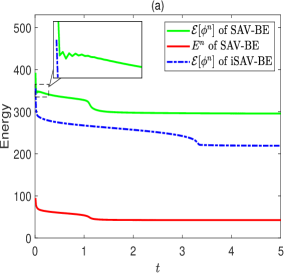
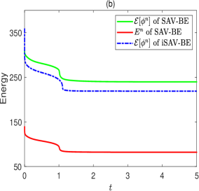
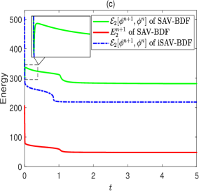
Figure 1. (Example 4.2): Time evolutions of the energy in SAV and iSAV. (a): BE schemes with $\tau=0.01$; (b): BE schemes with $\tau=0.001$; (c): BDF schemes with $\tau=0.001$.

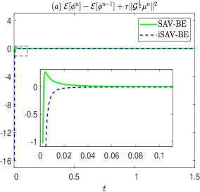
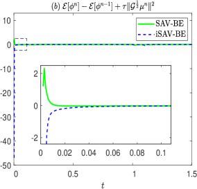
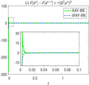
Figure 2. (Example 4.2): Time evolution of $\mathcal{E}[\phi^{n}]-\mathcal{E}[\phi^{n-1}]+\tau\|\mathcal{G}^{\frac{1}{2}}\mu^{n}\|^{2}$ in SAV-BE and iSAV-BE with $\tau=0.001$. (a) $\varepsilon=0.1$; (b) $\varepsilon=0.04$; (c) $\varepsilon=0.01$.

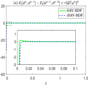
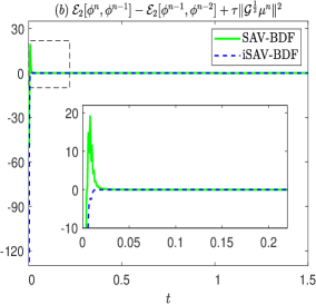
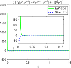
Figure 3. (Example 4.2): Time evolution of $\mathcal{E}_{2}[\phi^{n},\phi^{n-1}]-\mathcal{E}_{2}[\phi^{n-1},\phi^{n-2}]+\tau\|\mathcal{G}^{\frac{1}{2}}\mu^{n}\|^{2}$ of SAV-BDF and iSAV-BDF with $\tau=0.001$. (a) $\varepsilon=0.1$; (b) $\varepsilon=0.04$; (c) $\varepsilon=0.01$.

Example 4.2 (Energy stability and comparison).

Now we take an example of the Cahn-Hilliard equation to test the energy stability of iSAV and make some comparisons with SAV. Set the computational domain $\Omega=[0,6.4]\times[0,6.4]$ with a $256\times 256$ spatial grid and the parameters as $\gamma=0.01,\,\alpha=1.$ The stabilizing parameter is chosen as $S=3/\varepsilon^{2}$ for iSAV. The initial data of (2.1) is given as

$$\phi(x,y,0)=\left\{\begin{aligned} &\;1,\qquad(x,y)\in\Omega_{0},\\ &-1,\quad\,(x,y)\in\Omega/\Omega_{0},\end{aligned}\right.$$

where $\Omega_{0}=\big{\{}(x,y)\in\Omega\,:\,(|x-3.2|\leq 1\cap|y-3.2|\leq 1)\cup(|x-5|\leq 0.36\cap|y-5|\leq 0.36)\big{\}}$ is a set of two squares in $\Omega$. Moreover, in order to maintain a positive lower bound for $r[\phi]$, an additional constant $1$ has been added to the double-well potential $F(\phi)$. We solve the problem by the presented SAV and iSAV schemes under the same step size.

Firstly, we test the time evolution of the ‘energy’ under the numerical schemes, i.e., $\mathcal{E}[\phi^{n}],E^{n}$ for BE schemes and $\mathcal{E}_{2}[\phi^{n+1},\phi^{n}],E_{2}^{n+1}$ for BDF schemes. We fix $\varepsilon=0.04$ here and take two different $\tau$. Figure 1 depicts the results for each scheme. We can observe that when time step of the SAV schemes is not small enough ((a)&(c) in Figure 1), the original energy ($\mathcal{E}$ or $\mathcal{E}_{2}$) is not monotonically decreasing where oscillations or increments could occur. In contrast, the original energy dissipation is strictly maintained by the iSAV schemes. This justifies Theorem 2.1. Moreover, at the end of the evolution, the reached steady states by SAV possess higher energy level than iSAV.

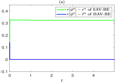
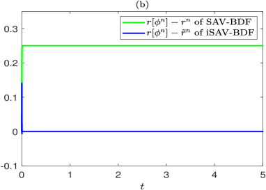
Figure 4. (Example 4.2): Difference between $r[\phi^{n}]$ and $r^{n}$ or $\tilde{r}^{n}$ in SAV or iSAV. (a): BE schemes with $\tau=0.001$; (b): BDF schemes with $\tau=0.001$.

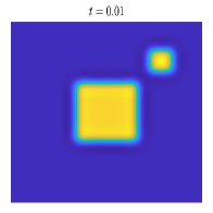
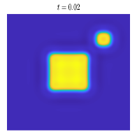
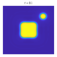
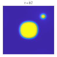
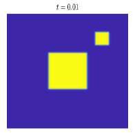
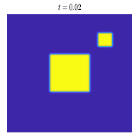
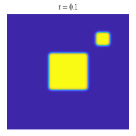
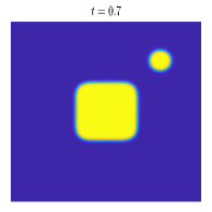
Figure 5. (Example 4.2) Contour plots of the numerical solution $\phi^{n}$ at $t=0.01$, $0.02$, $0.1$ and $0.7$ with $\tau=0.01$. Top: SAV-BE; Down: iSAV-BE.

To further demonstrate the improvement of iSAV, we test the energy decaying rate (2.3) under the schemes. For the BE schemes, we aim to visualize the difference between (2.6) and (2.11), especially when $\varepsilon$ decreases. Therefore, we plot the evolution of the quantity $\mathcal{E}[\phi^{n}]-\mathcal{E}[\phi^{n-1}]+\tau\|\mathcal{G}^{\frac{1}{2}}\mu^{n}\|^{2}$ in Figure 2 for three different $\varepsilon$. We can see that the result from iSAV remains monotone and non-positive, while the result from SAV becomes positive and contains oscillations that become stronger as $\varepsilon$ reduces. For the BDF schemes, we test (2.19) and the results of $\mathcal{E}_{2}[\phi^{n},\phi^{n-1}]-\mathcal{E}_{2}[\phi^{n-1},\phi^{n-2}]+\tau\|\mathcal{G}^{\frac{1}{2}}\mu^{n}\|^{2}$ are given in Figure 3, where the proposed iSAV-BDF always produce non-positive results.

In addition, we address Remarks 2 and 4 by computing the error $r[\phi^{n}]-r^{n}$ in SAV and the error $r[\phi^{n}]-\tilde{r}^{n}$ in iSAV. With $\varepsilon=0.04$ and $\tau=0.001$ fixed, the results are displayed in Figure 4. It can be observed that in the iSAV schemes, the difference between the introduced auxiliary variable and the original variable is indeed much smaller than that of SAV schemes. At last, we show the contour plots of the numerical solutions from SAV-BE and iSAV-BE in Figure 5. Here the SAV-BE without stabilization terms, as reported in [30, 34], exhibits spurious oscillations at the early stage of the solution, while iSAV-BE does not.

Last but not least, we use this example to address Remark 6 on the technical condition about $\tau$. We solve the problem under three different $\varepsilon$ with $S=3/\varepsilon^{2}$, and we fix $\tau=0.1$ for iSAV-BE. The results given in Figure 6 show that iSAV-BE can have the original energy-stability for large $\tau$ not restricted by $S$ or $\varepsilon$.

Based on the above findings and comparisons, we can conclude that the proposed iSAV schemes are stable, accurate and can indeed gain practical improvements.

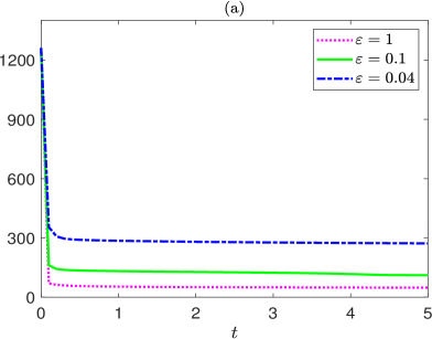
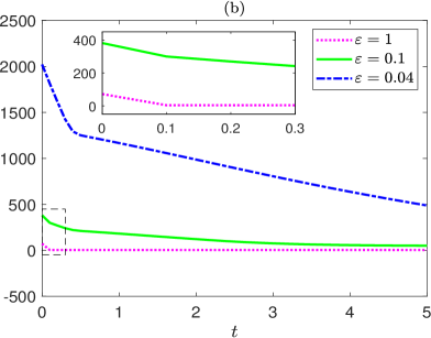
Figure 6. (Example 4.2 and 4.3): Time evolution of original energy of iSAV-BE under a fixed $\tau=0.1$ for different $\varepsilon$. (a) Example 4.2; (b) Example 4.3.

4.2. Flory-Huggins (F-H) potential

Next, we consider the Flory-Huggins type potential [2, 16], i.e.,

$$F(\phi)=\frac{1}{\varepsilon^{2}}\left[\phi\,{\rm ln}\phi+\left(1-\phi\right)\,{\rm ln}(1-\phi)+\beta\left(\phi-\phi^{2}\right)\right],$$

which is a popular class of logarithmic potentials in applications for (2.1). In the F-H potential, the domain of definition is an open interval $(0,1)$, and so the numerical solution needs to be strictly confined within this domain to avoid calculation overflow, which is more challenging. A helpful regularization strategy to the problem can be introduced by extending the domain $(0,1)$ to $(-\infty,\infty)$ and replacing the logarithmic function for (2.1) by a $C^{2}$-continuous, convex, and piecewisely defined function [10, 51]: for some $0<\sigma\leq\frac{1}{2}$,

$$F(\phi)=\frac{1}{\varepsilon^{2}}\left\{\begin{array}[]{ll}\phi\,{\rm ln}\phi+\frac{\left(1-\phi\right)^{2}}{2\sigma}+(1-\phi)\,{\rm ln}\sigma-\frac{\sigma}{2}+\beta\left(\phi-\phi^{2}\right),&{\rm if}\;\;\phi\geq 1-\sigma,\\ \phi\,{\rm ln}\phi+\left(1-\phi\right)\,{\rm ln}(1-\phi)+\beta\left(\phi-\phi^{2}\right),&{\rm if}\;\;\sigma\leq\phi\leq 1-\sigma,\\ (1-\phi)\,{\rm ln}(1-\phi)+\frac{\phi^{2}}{2\sigma}+\phi\,{\rm ln}\sigma-\frac{\sigma}{2}+\beta\left(\phi-\phi^{2}\right),&{\rm if}\;\;\phi\leq\sigma.\end{array}\right.$$

We shall show by this subsection that the proposed iSAV schemes (present only results of BE for simplicity) work well for (2.1) with the logarithmic potential under such strategy.

Example 4.3.

We consider the $H^{-\alpha}$ flow ($\alpha=0\;{\rm or}\;1$) with parameters $\varepsilon=0.04,\,\gamma=0.5,\,\beta=3,\,\sigma=0.01,\,S=10/\varepsilon^{2}$ and the computational domain $\Omega=[0,2\pi]\times[0,2\pi]$ with a $256\times 256$ spatial discrete grid. The initial value of (2.1) is given as

$$\phi(x,y,0)=\left\{\begin{aligned} &0.7,\qquad(x,y)\in\Omega_{0},\\ &0.3,\qquad(x,y)\in\Omega/\Omega_{0},\end{aligned}\right.$$

where $\Omega_{0}=\big{\{}(x,y)\in\Omega\,:\,(|x-x_{1}|^{2}\leq 1.4^{2}\cap|y-y_{1}|\leq 1.4^{2})\cup(|x-x_{2}|^{2}\leq 0.5^{2}\cap|y-y_{2}|\leq 0.5^{2})\big{\}}$ denotes two disk regions centered at $(x_{1},y_{1})=(\pi-0.8,\pi)$ and $(x_{2},y_{2})=(\pi+1.7,\pi)$. To maintain a positive lower bound for $r[\phi]$, an additional constant $0.06/\varepsilon^{2}$ has been added in $F(\phi)$.

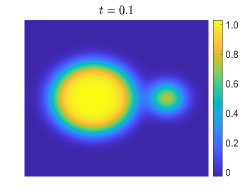
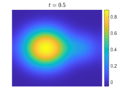
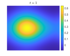
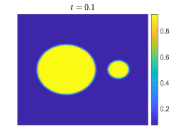
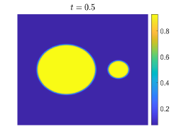
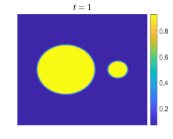
Figure 7. (Example 4.3, $\alpha=0$) Contour plots of the numerical solutions $\phi^{n}$ at $t=0.1$, $0.5$ and $1.0$ with $\tau=0.01$. Top: SAV-BE; Down: iSAV-BE.

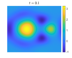
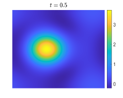
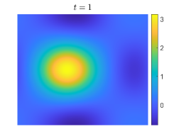
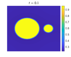
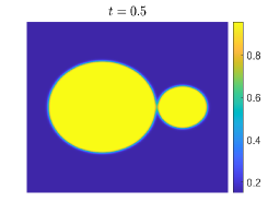
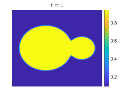
Figure 8. (Example 4.3, $\alpha=1$) Contour plots of numerical solutions $\phi^{n}$ at $t=0.1$, $0.5$ and $1.0$ with $\tau=0.01$. Top: SAV-BE; Down: iSAV-BE.

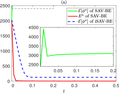
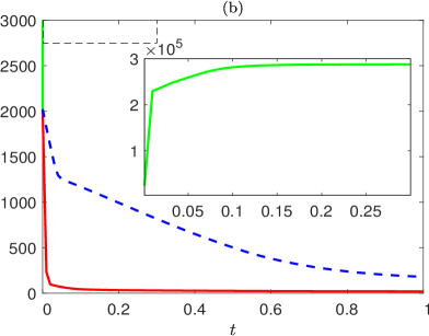
Figure 9. (Example 4.3): Time evolution of the energy of SAV-BE and iSAV-BE with $\tau=0.01$. (a) $\alpha=0$; (b) $\alpha=1$.

With $\tau=0.01$ fixed, Figures 7 and 8 display the numerical solutions obtained by SAV-BE and iSAV-BE at different time for Allen-Cahn model and Cahn-Hilliard model, respectively. Figure 9 shows the energy evolution of each scheme. From the numerical results, we can observe that the SAV schemes (without stabilization) exhibit the similar instability issue as before and the problem seems severer in the case of F-H potential. Numerical solutions of SAV-BE can exceed the interval $(0,1)$ (1st line of Figure 8), resulting in false states with significant increase in the original energy (Figure 9). These phenomena do not occur in iSAV. The performance of iSAV-BE with large $\tau$ free from $\varepsilon$ under this example is included in Figure 6.

Example 4.4.

With all other parameters same as in Example 4.3, we now consider a random initial data:

$$\phi(x,y,0)=0.5+0.2\,{\rm Rand}(x,y),$$

where ${\rm Rand}(x,y)$ stands for randomly generated values in $[-1,1]$ under the uniform distribution.

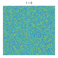
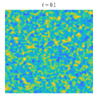
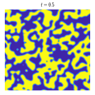
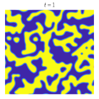
Figure 10. (Example 4.4, $\alpha=0$) Contour plots of the numerical solutions $\phi^{n}$ from iSAV-BE at $t=0$, $0.1$, $0.5$ and $1$ with $\tau=0.01$.

Figure 10 displays the states of the $H^{0}$ flow obtained by the iSAV-BE scheme at different time. We can observe that although the initial value for (2.1) is extremely rough, the iSAV scheme still works well, where the coarsening process can be captured. This indicates the smoothness assumption in the theorem is technical.

5. Conclusion

This paper proposed some linear numerical schemes for solving gradient flows under the framework of the scalar auxiliary variable (SAV) approach, where we aimed to improve the stability of the original energy of the problem. In particular, a first-order improved SAV (iSAV) scheme which involves no nonlinear equations, was constructed and was rigorously proved to offer the original energy-dissipation. Convergence analysis with the optimal error bound has been established for it. Numerical results validated the theoretical accuracy and original energy stability of the proposed iSAV scheme, and extensive comparisons with SAV were made to illustrate the gain. The possible second-order extension was also suggested and supported by numerical experiments.

Appendix A Derivation of (2.6).

Assume that $\phi^{n}\;(n=0,1,\cdots)$, $\phi_{t}$, $f$ and $f^{\prime}$ are all bounded. By direct calculations and (2.5), we have

$$\frac{1}{\tau}\left(\mathcal{E}[\phi^{n+1}]-\mathcal{E}[\phi^{n}]\right)= \frac{1}{\tau}\left(E^{n+1}-E^{n}\right)+\frac{1}{\tau}\left(\mathcal{E}[\phi^{n+1}]-E^{n+1}\right)-\frac{1}{\tau}\left(\mathcal{E}[\phi^{n}]-E^{n}\right)$$

$$\leq -\left\|\mathcal{G}^{\frac{1}{2}}\mu^{n+1}\right\|^{2}+\frac{1}{\tau}\left[\left(r[\phi^{n+1}]\right)^{2}-\left(r^{n+1}\right)^{2}-\left(r[\phi^{n}]\right)^{2}+\left(r^{n}\right)^{2}\right].$$ (A.1)

Then by (2.4c) and (2.14), we can derive

$$\left(r[\phi^{n+1}]\right)^{2}-\left(r^{n+1}\right)^{2}-\left(r[\phi^{n}]\right)^{2}+\left(r^{n}\right)^{2}=\frac{r[\phi^{n}]-r^{n}}{\sqrt{\mathcal{F}[\phi^{n}]}}\int_{\Omega}{f(\phi^{n})\left(\phi^{n+1}-\phi^{n}\right)}\,{\rm d}{\bf x}$$

$$\hskip 42.67912pt+\frac{1}{2}\int_{\Omega}{f^{\prime}\left((1-\rho_{1})\phi^{n}+\rho_{1}\phi^{n+1}\right)(\phi^{n+1}-\phi^{n})^{2}}\,{\rm d}{\bf x}-\frac{1}{4\mathcal{F}[\phi^{n}]}\left[\int_{\Omega}{f(\phi^{n})\left(\phi^{n+1}-\phi^{n}\right)}\,{\rm d}{\bf x}\right]^{2}=\mathcal{O}(\tau^{2}),$$

where the last equality made use of the convergence result of (2.4) from [33]. Plugging the above into (A.1), we can obtain (2.6).

Appendix B Derivation of (2.19).

Firstly, by taking the $L^{2}$ inner product of (2.18a) with $\mu^{n+1}$, we have

$$\frac{1}{2\tau}\left\langle 3\phi^{n+1}-4\phi^{n}+\phi^{n-1},\mu^{n+1}\right\rangle=-\left\|\mathcal{G}^{\frac{1}{2}}\mu^{n+1}\right\|^{2}.$$ (B.1)

Secondly, by taking the $L^{2}$ inner product of (2.18b) with $(3\phi^{n+1}-4\phi^{n}+\phi^{n-1})/2\tau$, and using the identities

$$2\langle\mathcal{L}u_{1},3u_{1}-4u_{2}+u_{3}\rangle=\left\|\mathcal{L}^{\frac{1}{2}}u_{1}\right\|^{2}-\left\|\mathcal{L}^{\frac{1}{2}}u_{2}\right\|^{2}+\left\|\mathcal{L}^{\frac{1}{2}}(2u_{1}-u_{2})\right\|^{2}-\left\|\mathcal{L}^{\frac{1}{2}}(2u_{2}-u_{3})\right\|^{2}$$

$$\hskip 113.81102pt+\left\|\mathcal{L}^{\frac{1}{2}}(u_{1}-2u_{2}+u_{3})\right\|^{2},$$

$$\langle u_{1}-2u_{2}+u_{3},3u_{1}-4u_{2}+u_{3}\rangle=\left\|u_{1}-u_{2}\right\|^{2}-\left\|u_{2}-u_{3}\right\|^{2}+2\left\|u_{1}-2u_{2}+u_{3}\right\|^{2},$$

for some general functions $u_{1},u_{2},u_{3}$, we can obtain

$$\frac{1}{2\tau}\left\langle\mu^{n+1},3\phi^{n+1}-4\phi^{n}+\phi^{n-1}\right\rangle$$

$$= \frac{1}{4\tau}\left(\left\|\mathcal{L}^{\frac{1}{2}}\phi^{n+1}\right\|^{2}-\left\|\mathcal{L}^{\frac{1}{2}}\phi^{n}\right\|^{2}+\left\|\mathcal{L}^{\frac{1}{2}}(2\phi^{n+1}-\phi^{n})\right\|^{2}-\left\|\mathcal{L}^{\frac{1}{2}}(2\phi^{n}-\phi^{n-1})\right\|^{2}\right.$$

$$\left.+\left\|\mathcal{L}^{\frac{1}{2}}(\phi^{n+1}-2\phi^{n}+\phi^{n-1})\right\|^{2}\right)+\frac{\tilde{r}^{n+1}}{2\tau}\left\langle\frac{f(\phi_{*}^{n+1})}{\sqrt{\mathcal{F}[\phi_{*}^{n+1}]}},3\phi^{n+1}-4\phi^{n}+\phi^{n-1}\right\rangle$$

$$+\frac{S}{2\tau}\left(\left\|\phi^{n+1}-\phi^{n}\right\|^{2}-\left\|\phi^{n}-\phi^{n-1}\right\|^{2}+2\left\|\phi^{n+1}-2\phi^{n}+\phi^{n-1}\right\|^{2}\right).$$ (B.2)

Thirdly, multiplying (2.18c) by $\tilde{r}^{n+1}/\tau$ and again by the identity, we can obtain that

$$\frac{1}{2\tau}\left[\left(\tilde{r}^{n+1}\right)^{2}-\left(r[\phi^{n}]\right)^{2}+\left(2\tilde{r}^{n+1}-r[\phi^{n}]\right)^{2}-\left(2r[\phi^{n}]-r[\phi^{n-1}]\right)^{2}+\left(\tilde{r}^{n+1}-2r[\phi^{n}]+r[\phi^{n-1}]\right)^{2}\right]$$

$$= \frac{\tilde{r}^{n+1}}{2\tau}\left\langle\frac{f(\phi_{*}^{n+1})}{\sqrt{\mathcal{F}[\phi_{*}^{n+1}]}},3\phi^{n+1}-4\phi^{n}+\phi^{n-1}\right\rangle.$$ (B.3)

Combining (B.1), (B.2) and (B.3), we have

$$\frac{1}{\tau}\left(\tilde{E}_{2}^{n+1}-\mathcal{E}_{2}[\phi^{n},\phi^{n-1}]\right)=-\left\|\mathcal{G}^{\frac{1}{2}}\mu^{n+1}\right\|^{2}-\mathcal{N}^{n}-\frac{S}{\tau}\left\|\phi^{n+1}-2\phi^{n}+\phi^{n-1}\right\|^{2},$$ (B.4)

with $\tilde{E}_{2}^{n+1}$ and $\mathcal{N}^{n}$ defined as

$$\tilde{E}_{2}^{n+1}=\frac{1}{4}\left(\left\|\mathcal{L}^{\frac{1}{2}}\phi^{n+1}\right\|^{2}+\left\|\mathcal{L}^{\frac{1}{2}}(2\phi^{n+1}-\phi^{n})\right\|^{2}\right)+\frac{1}{2}\left[\left(\tilde{r}^{n+1}\right)^{2}+\left(2\tilde{r}^{n+1}-r[\phi^{n}]\right)^{2}\right]+\frac{S}{2}\left\|\phi^{n+1}-\phi^{n}\right\|^{2},$$

$$\mathcal{N}^{n}=\frac{1}{4\tau}\left\|\mathcal{L}^{\frac{1}{2}}(\phi^{n+1}-2\phi^{n}+\phi^{n-1})\right\|^{2}+\frac{1}{2\tau}\left(\tilde{r}^{n+1}-2r[\phi^{n}]+r[\phi^{n-1}]\right)^{2}.$$

On the other hand, we have

$$\frac{1}{\tau}\left(\mathcal{E}_{2}[\phi^{n+1},\phi^{n}]-\tilde{E}_{2}^{n+1}\right)= \frac{1}{2\tau}\left[\left(r[\phi^{n+1}]\right)^{2}-\left(\tilde{r}^{n+1}\right)^{2}+\left(2r[\phi^{n+1}]-r[\phi^{n}]\right)^{2}-\left(2\tilde{r}^{n+1}-r[\phi^{n}]\right)^{2}\right]$$

$$= \frac{1}{2\tau}\left(r[\phi^{n+1}]-\tilde{r}^{n+1}\right)\left(5r[\phi^{n+1}]+5\tilde{r}^{n+1}-4r[\phi^{n}]\right).$$ (B.5)

Then, we compute the difference between $r[\phi^{n+1}]$ and $\tilde{r}^{n+1}$. By setting $\phi=\phi_{*}^{n+1}$, $\psi=\phi^{n+1}-2\phi^{n}+\phi^{n-1}$, $\rho=1$ and $k=1$ in (3.24), we have

$$r[\phi^{n+1}]= r[\phi_{*}^{n+1}+(\phi^{n+1}-2\phi^{n}+\phi^{n-1})]$$

$$= r[\phi_{*}^{n+1}]+\frac{1}{2\sqrt{\mathcal{F}[\phi_{*}^{n+1}]}}\int_{\Omega}{f(\phi_{*}^{n+1})(\phi^{n+1}-2\phi^{n}+\phi^{n-1})}\,{\rm d}{\bf x}+\mathcal{X}_{1}^{n},$$ (B.6)

where

$$\mathcal{X}_{1}^{n}=\frac{1}{4}\big{(}\mathcal{E}_{1}[\xi_{0}^{n}]\big{)}^{-\frac{1}{2}}\int_{\Omega}{f^{\prime}(\xi_{0}^{n})(\phi^{n+1}-2\phi^{n}+\phi^{n-1})^{2}}\,{\rm d}{\bf x}-\frac{1}{8}\big{(}\mathcal{E}_{1}[\xi_{0}^{n}]\big{)}^{-\frac{3}{2}}\Big{(}\int_{\Omega}{f(\xi_{0}^{n})(\phi^{n+1}-2\phi^{n}+\phi^{n-1})}\,{\rm d}{\bf x}\Big{)}^{2},$$

with $\xi_{0}^{n}=\rho_{0}\phi^{n+1}+2(1-\rho_{0})\phi^{n}+(\rho_{0}-1)\phi^{n-1}$ for some $\rho_{0}\in(0,1)$. And by setting $\phi=\phi_{*}^{n+1}$, $\psi=\phi^{n}-\phi^{n-1}$, $\rho=-1,-2$ and $k=2$ in (3.24), there are

$$r[\phi^{n}]= r[\phi_{*}^{n+1}-\psi]=r[\phi_{*}^{n+1}]-\frac{1}{2\sqrt{\mathcal{F}[\phi_{*}^{n+1}]}}\int_{\Omega}{f(\phi_{*}^{n+1})(\phi^{n}-\phi^{n-1})}\,{\rm d}{\bf x}$$

$$\qquad\qquad\qquad+\frac{1}{2}\frac{{\rm d}^{2}}{{\rm d}\rho^{2}}r[\phi_{*}^{n+1}+\rho(\phi^{n}-\phi^{n-1})]\Big{|}_{\rho=0}-\frac{1}{6}\frac{{\rm d}^{3}}{{\rm d}\rho^{3}}r[\phi_{*}^{n+1}+\rho(\phi^{n}-\phi^{n-1})]\Big{|}_{\rho=\rho_{1}},$$ (B.7)

$$r[\phi^{n-1}]= r[\phi_{*}^{n+1}-2\psi]=r[\phi_{*}^{n+1}]-\frac{1}{\sqrt{\mathcal{F}[\phi_{*}^{n+1}]}}\int_{\Omega}{f(\phi_{*}^{n+1})(\phi^{n}-\phi^{n-1})}\,{\rm d}{\bf x}$$

$$\qquad\qquad\qquad+2\frac{{\rm d}^{2}}{{\rm d}\rho^{2}}r[\phi_{*}^{n+1}+\rho(\phi^{n}-\phi^{n-1})]\Big{|}_{\rho=0}-\frac{4}{3}\frac{{\rm d}^{3}}{{\rm d}\rho^{3}}r[\phi_{*}^{n+1}+\rho(\phi^{n}-\phi^{n-1})]\Big{|}_{\rho=\rho_{2}},$$ (B.8)

for some $\rho_{1}\in(-1,0)$, $\rho_{2}\in(-2,0)$. Combining (B.6), (B.7) and (B.8), one can obtain

$$3r[\phi^{n+1}]-4r[\phi^{n}]+r[\phi^{n-1}]=\frac{1}{2\sqrt{\mathcal{F}[\phi_{*}^{n+1}]}}\int_{\Omega}{f(\phi_{*}^{n+1})(3\phi^{n+1}-4\phi^{n}+\phi^{n-1})}\,{\rm d}{\bf x}+\mathcal{X}_{1}^{n}+\mathcal{X}_{2}^{n}+\mathcal{X}_{3}^{n},$$ (B.9)

where the residuals $\mathcal{X}_{2}^{n}$ and $\mathcal{X}_{3}^{n}$ denote

$$\mathcal{X}_{2}^{n}= \frac{1}{4}\left(\mathcal{F}[\xi_{1}^{n}]\right)^{-\frac{5}{2}}\left(\int_{\Omega}{f(\xi_{1}^{n})(\phi^{n}-\phi^{n-1})}\,{\rm d}{\bf x}\right)^{3}-\frac{1}{2}\left(\mathcal{F}[\xi_{1}^{n}]\right)^{-\frac{3}{2}}\left(\int_{\Omega}{f(\xi_{1}^{n})(\phi^{n}-\phi^{n-1})}\,{\rm d}{\bf x}\right)$$

$$\times\left(\int_{\Omega}{f^{\prime}(\xi_{1}^{n})(\phi^{n}-\phi^{n-1})^{2}}\,{\rm d}{\bf x}\right)+\frac{1}{3}\left(\mathcal{F}[\xi_{1}^{n}]\right)^{-\frac{1}{2}}\int_{\Omega}{f^{\prime\prime}(\xi_{1}^{n})(\phi^{n}-\phi^{n-1})^{3}}\,{\rm d}{\bf x},$$

$$\mathcal{X}_{3}^{n}= -\frac{1}{2}\left(\mathcal{F}[\xi_{2}^{n}]\right)^{-\frac{5}{2}}\left(\int_{\Omega}{f(\xi_{2}^{n})(\phi^{n}-\phi^{n-1})}\,{\rm d}{\bf x}\right)^{3}+\left(\mathcal{F}[\xi_{2}^{n}]\right)^{-\frac{3}{2}}\left(\int_{\Omega}{f(\xi_{2}^{n})(\phi^{n}-\phi^{n-1})}\,{\rm d}{\bf x}\right)$$

$$\times\left(\int_{\Omega}{f^{\prime}(\xi_{2}^{n})(\phi^{n}-\phi^{n-1})^{2}}\,{\rm d}{\bf x}\right)-\frac{2}{3}\left(\mathcal{F}[\xi_{2}^{n}]\right)^{-\frac{1}{2}}\int_{\Omega}{f^{\prime\prime}(\xi_{2}^{n})(\phi^{n}-\phi^{n-1})^{3}}\,{\rm d}{\bf x},$$

with $\xi_{1}^{n}=(2+\rho_{1})\phi^{n}+(1+\rho_{1})\phi^{n-1},\ \xi_{2}^{n}=(2+\rho_{2})\phi^{n}+(1+\rho_{2})\phi^{n-1}$. Subtracting (2.18c) from (B.9) and concerning the second-order accuracy of iSAV-BDF scheme, we find formally

$$r[\phi^{n+1}]-\tilde{r}^{n+1}=\frac{1}{3}\left(\mathcal{X}_{1}^{n}+\mathcal{X}_{2}^{n}+\mathcal{X}_{3}^{n}\right)=\mathcal{O}(\tau^{3}).$$ (B.10)

Combining (B.4), (B.5) and (B.10), we can derive that

$$\frac{1}{\tau}\left(\mathcal{E}_{2}[\phi^{n+1},\phi^{n}]-\mathcal{E}_{2}[\phi^{n},\phi^{n-1}]\right)$$

$$= \frac{1}{\tau}\left(\tilde{E}_{2}^{n+1}-\mathcal{E}_{2}[\phi^{n},\phi^{n-1}]\right)+\frac{1}{\tau}\left(\mathcal{E}_{2}[\phi^{n+1},\phi^{n}]-\tilde{E}_{2}^{n+1}\right)$$

$$= -\left\|\mathcal{G}^{\frac{1}{2}}\mu^{n+1}\right\|^{2}-\mathcal{N}^{n}-\frac{S}{\tau}\left\|\phi^{n+1}-2\phi^{n}+\phi^{n-1}\right\|^{2}+\frac{1}{2\tau}\left(r[\phi^{n+1}]-\tilde{r}^{n+1}\right)\left(5r[\phi^{n+1}]+5\tilde{r}^{n+1}-4r[\phi^{n}]\right)$$

$$\leq -\left\|\mathcal{G}^{\frac{1}{2}}\mu^{n+1}\right\|^{2}+\mathcal{O}(\tau^{2}),$$

which gives (2.19).

References

- [1] D. M. Anderson, G. B. McFadden, and A. A. Wheeler, Diffuse-interface methods in fluid mechanics, Annual Review of Fluid Mechanics, 30 (1998), pp. 139–165.
- [2] K. Binder, Collective diffusion, nucleation, and spinodal decomposition in polymer mixtures, The Journal of Chemical Physics, 79 (1983), pp. 6387–6409.
- [3] C. Chen and X. Yang, Fast, provably unconditionally energy stable, and second-order accurate algorithms for the anisotropic Cahn–Hilliard model, Computer Methods in Applied Mechanics and Engineering, 351 (2019), pp. 35–59.
- [4] R. Chen and S. Gu, On novel linear schemes for the Cahn–Hilliard equation based on an improved invariant energy quadratization approach, Journal of Computational and Applied Mathematics, 414 (2022), p. 114405.
- [5] R. Chen, G. Ji, X. Yang, and H. Zhang, Decoupled energy stable schemes for phase-field vesicle membrane model, Journal of Computational Physics, 302 (2015), pp. 509–523.
- [6] R. Chen, X. Yang, and H. Zhang, Second order, linear, and unconditionally energy stable schemes for a hydrodynamic model of smectic-A liquid crystals, SIAM Journal on Scientific Computing, 39 (2017), pp. A2808–A2833.
- [7] W. Chen, W. Feng, Y. Liu, C. Wang, and S. M. Wise, A second order energy stable scheme for the Cahn-Hilliard-Hele-Shaw equations, Discrete and Continuous Dynamical Systems-Series B, 24 (2019), pp. 149–182.
- [8] Q. Cheng, C. Liu, and J. Shen, A new lagrange multiplier approach for gradient flows, Computer Methods in Applied Mechanics and Engineering, 367 (2020), p. 113070.
- [9] Q. Cheng, C. Liu, and J. Shen, Generalized SAV approaches for gradient systems, Journal of Computational and Applied Mathematics, 394 (2021), p. 113532.
- [10] M. I. M. Copetti and C. M. Elliott, Numerical analysis of the Cahn-Hilliard equation with a logarithmic free energy, Numerische Mathematik, 63 (1992), pp. 39–65.
- [11] Q. Du and X. Feng, The phase field method for geometric moving interfaces and their numerical approximations, Handbook of Numerical Analysis, 21 (2020), pp. 425–508.
- [12] Q. Du, L. Ju, X. Li, and Z. Qiao, Maximum bound principles for a class of semilinear parabolic equations and exponential time-differencing schemes, SIAM Review, 63 (2021), p. 317–359.
- [13] K. Elder, M. Katakowski, M. Haataja, and M. Grant, Modeling elasticity in crystal growth, Physical Review Letters, 88 (2002), p. 245701.
- [14] C. M. Elliott and A. Stuart, The global dynamics of discrete semilinear parabolic equations, SIAM Journal on Numerical Analysis, 30 (1993), pp. 1622–1663.
- [15] D. J. Eyre, Unconditionally gradient stable time marching the Cahn-Hilliard equation, MRS Online Proceedings Library (OPL), 529 (1998), p. 39.
- [16] M. Fiałkowski and R. Hołyst, Dynamics of phase separation in polymer blends revisited: morphology, spinodal, noise, and nucleation, Macromolecular Theory and Simulations, 17 (2008), pp. 263–273.
- [17] J. Fraaije, Dynamic density functional theory for microphase separation kinetics of block copolymer melts, The Journal of Chemical Physics, 99 (1993), pp. 9202–9212.
- [18] J. Fraaije and G. Sevink, Model for pattern formation in polymer surfactant nanodroplets, Macromolecules, 36 (2003), pp. 7891–7893.
- [19] M. E. Gurtin, D. Polignone, and J. Vinals, Two-phase binary fluids and immiscible fluids described by an order parameter, Mathematical Models and Methods in Applied Sciences, 6 (1996), pp. 815–831.
- [20] F. Huang and J. Shen, A new class of implicit–explicit BDFk SAV schemes for general dissipative systems and their error analysis, Computer Methods in Applied Mechanics and Engineering, 392 (2022), p. 114718.
- [21] F. Huang, J. Shen, and Z. Yang, A highly efficient and accurate new scalar auxiliary variable approach for gradient flows, SIAM Journal on Scientific Computing, 42 (2020), pp. A2514–A2536.
- [22] M. Jiang, Z. Zhang, and J. Zhao, Improving the accuracy and consistency of the scalar auxiliary variable (SAV) method with relaxation, Journal of Computational Physics, 456 (2022), p. 110954.
- [23] L. Ju, X. Li, Z. Qiao, and H. Zhang, Energy stability and error estimates of exponential time differencing schemes for the epitaxial growth model without slope selection, Mathematics of Computation, 87 (2018), pp. 1859–1885.
- [24] R. Larson, Arrested tumbling in shearing flows of liquid-crystal polymers, Macromolecules, 23 (1990), pp. 3983–3992.
- [25] F. M. Leslie, Theory of flow phenomena in liquid crystals, in Advances in Liquid Crystals, vol. 4, Elsevier, 1979, pp. 1–81.
- [26] D. Li and Z. Qiao, On second order semi-implicit Fourier spectral methods for 2d Cahn–Hilliard equations, Journal of Scientific Computing, 70 (2017), pp. 301–341.
- [27] Z. Liu and Q. He, A novel relaxed scalar auxiliary variable approach for gradient flows, Applied Mathematics Letters, 141 (2023), p. 108613.
- [28] Z. Liu and X. Li, The exponential scalar auxiliary variable (E-SAV) approach for phase field models and its explicit computing, SIAM Journal on Scientific Computing, 42 (2020), pp. B630–B655.
- [29] J. Lowengrub and L. Truskinovsky, Quasi–incompressible Cahn–Hilliard fluids and topological transitions, Proceedings of the Royal Society of London. Series A: Mathematical, Physical and Engineering Sciences, 454 (1998), pp. 2617–2654.
- [30] J. Shen, Efficient and accurate structure preserving schemes for complex nonlinear systems, in Handbook of Numerical Analysis, vol. 20, Elsevier, 2019, pp. 647–669.
- [31] J. Shen, T. Tang, and L.-L. Wang, Spectral methods: algorithms, analysis and applications, vol. 41, Springer Science & Business Media, 2011.
- [32] J. Shen, C. Wang, X. Wang, and S. M. Wise, Second-order convex splitting schemes for gradient flows with Ehrlich–Schwoebel type energy: application to thin film epitaxy, SIAM Journal on Numerical Analysis, 50 (2012), pp. 105–125.
- [33] J. Shen and J. Xu, Convergence and error analysis for the scalar auxiliary variable (SAV) schemes to gradient flows, SIAM Journal on Numerical Analysis, 56 (2018), pp. 2895–2912.
- [34] J. Shen, J. Xu, and J. Yang, A new class of efficient and robust energy stable schemes for gradient flows, SIAM Review, 61 (2019), pp. 474–506.
- [35] J. Shen and X. Yang, Numerical approximations of Allen-Cahn and Cahn-Hilliard equations, Discrete and Continuous Dynamical Systems, 28 (2010), pp. 1669–1691.
- [36] J. Shen and X. Yang, Decoupled energy stable schemes for phase-field models of two-phase complex fluids, SIAM Journal on Scientific Computing, 36 (2014), pp. B122–B145.
- [37] J. Shen and X. Yang, Decoupled, energy stable schemes for phase-field models of two-phase incompressible flows, SIAM Journal on Numerical Analysis, 53 (2015), pp. 279–296.
- [38] J. Shen, X. Yang, and H. Yu, Efficient energy stable numerical schemes for a phase field moving contact line model, Journal of Computational Physics, 284 (2015), pp. 617–630.
- [39] A. Takhirov, Quad-SAV scheme for gradient systems, Journal of Computational and Applied Mathematics, 443 (2024), p. 115768.
- [40] R. Temam, Infinite-dimensional dynamical systems in mechanics and physics, vol. 68, Springer Science & Business Media, 2012.
- [41] X. Wang, L. Ju, and Q. Du, Efficient and stable exponential time differencing Runge–Kutta methods for phase field elastic bending energy models, Journal of Computational Physics, 316 (2016), pp. 21–38.
- [42] S. M. Wise, Unconditionally stable finite difference, nonlinear multigrid simulation of the Cahn-Hilliard-Hele-Shaw system of equations, Journal of Scientific Computing, 44 (2010), pp. 38–68.
- [43] Z. Xu, X. Yang, H. Zhang, and Z. Xie, Efficient and linear schemes for anisotropic Cahn–Hilliard model using the stabilized-invariant energy quadratization (S-IEQ) approach, Computer Physics Communications, 238 (2019), pp. 36–49.
- [44] X. Yang, Linear, first and second-order, unconditionally energy stable numerical schemes for the phase field model of homopolymer blends, Journal of Computational Physics, 327 (2016), pp. 294–316.
- [45] X. Yang and L. Ju, Efficient linear schemes with unconditional energy stability for the phase field elastic bending energy model, Computer Methods in Applied Mechanics and Engineering, 315 (2017), pp. 691–712.
- [46] X. Yang and L. Ju, Linear and unconditionally energy stable schemes for the binary fluid–surfactant phase field model, Computer Methods in Applied Mechanics and Engineering, 318 (2017), pp. 1005–1029.
- [47] X. Yang, J. Zhao, and Q. Wang, Numerical approximations for the molecular beam epitaxial growth model based on the invariant energy quadratization method, Journal of Computational Physics, 333 (2017), pp. 104–127.
- [48] X. Yang, J. Zhao, Q. Wang, and J. Shen, Numerical approximations for a three-component Cahn–Hilliard phase-field model based on the invariant energy quadratization method, Mathematical Models and Methods in Applied Sciences, 27 (2017), pp. 1993–2030.
- [49] Z. Yang and S. Dong, A roadmap for discretely energy-stable schemes for dissipative systems based on a generalized auxiliary variable with guaranteed positivity, Journal of Computational Physics, 404 (2020), p. 109121.
- [50] J. Zhang, C. Chen, X. Yang, Y. Chu, and Z. Xia, Efficient, non-iterative, and second-order accurate numerical algorithms for the anisotropic Allen–Cahn equation with precise nonlocal mass conservation, Journal of Computational Applied Mathematics, 363 (2020), pp. 444–463.
- [51] J. Zhang and X. Yang, Non-iterative, unconditionally energy stable and large time-stepping method for the Cahn-Hilliard phase-field model with Flory-Huggins-de Gennes free energy, Advances in Computational Mathematics, 46 (2020), pp. 1–27.