Doubly Robust Causal Effect Estimation under Networked Interference via Targeted Learning

Abstract

Causal effect estimation under networked interference is an important but challenging problem. Available parametric methods are limited in their model space, while previous semiparametric methods, e.g., leveraging neural networks to fit only one single nuisance function, may still encounter misspecification problems under networked interference without appropriate assumptions on the data generation process. To mitigate bias stemming from misspecification, we propose a novel doubly robust causal effect estimator under networked interference, by adapting the targeted learning technique to the training of neural networks. Specifically, we generalize the targeted learning technique into the networked interference setting and establish the condition under which an estimator achieves double robustness. Based on the condition, we devise an end-to-end causal effect estimator by transforming the identified theoretical condition into a targeted loss. Moreover, we provide a theoretical analysis of our designed estimator, revealing a faster convergence rate compared to a single nuisance model. Extensive experimental results on two real-world networks with semisynthetic data demonstrate the effectiveness of our proposed estimators.

1 Introduction

Estimating causal effects under networked interference has drawn increasing attention across various domains such as human ecology (Ferraro et al., 2019), epidemiology (Barkley et al., 2020), advertisement (Parshakov et al., 2020), and so on. Networked interference arises when interconnected units impact each other, leading to a violation of the Stable Unit Treatment Value Assumption (SUTVA). For example, as shown in Figure 1, in epidemiology, preventive measures like vaccination can indirectly protect unvaccinated units due to the vaccinated individuals surrounding them. Consequently, the infection risk for a unit depends not only on its vaccination status but also on the vaccination statuses of neighboring units. Such networked interference breaks the SUTVA and leads to bias in traditional causal inference (Forastiere et al., 2021), making traditional estimand no longer applicable. To model the interference between units, different kinds of estimands can be defined, i.e., main effects (effects of units’ own treatments), spillover effects (effects of units’ treatments on other units), and total effects (combined main and spillover effects).

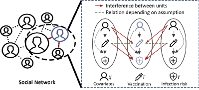
Figure 1: A toy example showing networked interference between units. The solid red and dashed green arrows, i.e., $\boldsymbol{\rightarrow}$ and $\boldsymbol{\dashrightarrow}$, mean the interaction from one to another unit. Whether the dashed green arrow $\boldsymbol{\dashrightarrow}$ exists depends on the assumption on DGP.

To estimate causal effects from observational networked data, a series of works have been proposed to remove the complex confounding bias introduced by networked interference. One standard way is utilizing the parametric regression including the neighbors’ covariate and treatment to model the nuisance function. In particular, Liu et al. (2016) propose covariate-adjustment methods using parametric regression on propensity scores for causal effect estimation. However, the parametric models are fragile and would yield bias once the model is misspecified, i.e., the designed model mismatches the data generation process (DGP). One of the remedies is to leverage the semiparametric regressions while exploring different assumptions on DGP. Specifically, by assuming that the networked interference is transmitted only through the neighbors’ statistic, Chin (2019); Ma & Tresp (2021); Cai et al. (2023) utilize different semiparametric regression to construct conditional outcome estimators for effect estimation. By assuming the conditional independence between the unit’s treatment and neighbors’ treatment, Forastiere et al. (2021) propose the joint generalized propensity score and devise a propensity score-based method for effect estimation under networked interference.

However, under networked interference, existing semiparametric estimators still encounter model misspecification due to inappropriate assumptions on the networked DGP, leading to biased effect estimation. Take Figure 1 as an example, let $t,x,t_{\mathcal{N}},x_{\mathcal{N}}$ be the treatment, the covariate, the neighbors’ treatment, and the neighbors’ covariate, respectively. Due to the interference between units, the generalized propensity model $p(t,t_{\mathcal{N}}|x,x_{\mathcal{N}})$ could have different alternative decomposition forms for the sake of estimating, e.g., $p(t|x,x_{\mathcal{N}})p(t_{\mathcal{N}}|x,x_{\mathcal{N}})$ or $p(t|x,x_{\mathcal{N}})p(t_{\mathcal{N}}|t,x,x_{\mathcal{N}})$ depending on whether the assumption $t\Vbar t_{\mathcal{N}}|x,x_{\mathcal{N}}$ holds. However, if the chosen decomposition mismatches the ground true DGP, the estimators will become inconsistent, resulting in biased estimated effects. To reduce the bias caused by misspecification, one attractive solution involves designing a doubly robust (DR) estimator via targeted learning. In this way, the consistent estimator can be achieved when one of the nuisance models is consistent. An essential question is raised: How can we design such an estimator to achieve lower bias under networked interference?

To answer the above question, we propose a doubly robust estimator, called TNet, for estimating causal effects under networked interference via targeted learning. First, under interference, to achieve double robustness, the traditional targeted technique (van der Laan & Rubin, 2006) can not be directly used since the data are no longer independent and identically distributed (i.i.d.). Second, considering the traditional three-step targeted estimator, we aim to adapt the targeted technique to our end-to-end neural network-based estimator, making it achieve double robustness and lower bias. Overall, we answer three specified questions: 1. What are good estimators under networked interference (see Section 4)? 2. How can we design targeted estimators with lower bias and double robustness property under networked interference (see Section 5)? 3. How fast a convergence rate can our designed estimator achieve (see Section 6)? Our solution and contribution can be summarized as follows:

• We develop an end-to-end effect estimator, by transforming the established theoretical condition into a targeted loss function, thus ensuring that our estimator maintains the attribute of double robustness in the presence of networked interference.

• We provide a theoretical analysis of the designed estimator, revealing its advantages in terms of convergence rate under mild assumptions.

• The extensive experimental results on two real-world networks demonstrate the correctness of our theory and the effectiveness of our model.

2 Related Works

Causal inference has been studied in two languages: the graphical models (Pearl, 2009) and the potential outcome framework (Rubin, 1974). The most related method is the propensity score method in the potential outcome framework, e.g., IPW method (Rosenbaum & Rubin, 1983; Rosenbaum, 1987), which is widely applied to many scenarios (Rosenbaum & Rubin, 1985; Li et al., 2018; Cai et al., 2024). There are also many outcome regression models, including meta-learners (Künzel et al., 2019), neural networks-based works (Johansson et al., 2016; Assaad et al., 2021). By incorporating them, one can construct a doubly robust estimator (Robins et al., 1994), i.e., the effect estimator is consistent as either the propensity model or the outcome repression model is consistent. Our work can be seen as an extension of DR estimators to the networked interference scenarios.

Causal inference under networked interference has drawn increasing attention recently. Liu et al. (2016) extend the traditional propensity score to account for neighbors’ treatments and features and propose a generalized Inverse Probability Weighting (IPW) estimator. Forastiere et al. (2021) define the joint propensity score and then propose a subclassification-based method. Drawing upon previous works, Lee et al. (2021) consider two IPW estimators and derive a closed-form estimator for the asymptotic variance. Based on the representation learning, Ma & Tresp (2021) add neighborhood exposure and neighbors’ features as additional input variables and applies HSIC to learn balanced representations. Jiang & Sun (2022) use adversarial learning to learn balanced representations for better effect estimation. Ma et al. (2022) propose a framework to learn causal effects on a hypergraph. (Cai et al., 2023) propose a reweighted representation learning method to learn balanced representations. Under networked interference, McNealis et al. (2023); Liu et al. (2023) propose an estimator to achieve DR property. Different from them, we adapt the targeted learning into our loss function, which might be more stable with the finite sample, and result in an end-to-end doubly robust estimator for causal effects under networked interference.

Targeted maximum likelihood estimation (TMLE) is a general framework to construct doubly robust, efficient, and substitution estimators (van der Laan & Rubin, 2006; Van der Laan et al., 2011). This technique is widely used in different settings, e.g., multiple time point interventions (van der Laan & Gruber, 2012), longitudinal data (Kreif et al., 2017), cluster-level exposure (Balzer et al., 2019), survival analysis (Chen et al., 2023). Moreover, designing targeted regularization is the most related issue. Shi et al. (2019) propose targeted regularization for binary treatment effect estimation. Nie et al. (2020) generalize the targeted regularization for continuous treatment estimation, which can be seen as a counterpart of our work without interference. Different from these works, we generalize the TMLE to a targeted loss that can be easily adapted into the training of nuisance functions under networked interference and correspondingly propose an end-to-end causal effect estimator under networked interference.

3 Notations, Assumptions, Esitimands

In this section, we start with the notations used in this work. Let $X\in\mathcal{X}$ be the covariate. Let $T\in\{0,1\}$ denote a binary treatment, where $T=1$ indicates a unit receives the treatment (treated) and $T=0$ indicates a unit receives no treatment (control). Let $Y\in\mathcal{Y}$ be the outcome. Let lowercase letters (e.g., $x,y,t$) denote the value of random variables. Let lowercase letters with subscript $i$ denote the value of the specified $i$-th unit. Thus, a network dataset is denoted as $D=(\{x_{i},t_{i},y_{i}\}_{i=1}^{n},E)$, where $E$ denotes the adjacency matrix of network and $n$ is the total number of units. We also denote $n_{1}$ and $n_{2}$ as the total number of treated units and control units, and thus $n=n_{1}+n_{2}$. We denote the set of first-order neighbors of $i$ as $\mathcal{N}_{i}$. We denote the treatment and feature vectors received by unit $i$’s neighbors as $t_{\mathcal{N}_{i}}$ and $x_{\mathcal{N}_{i}}$. Due to the presence of networked interference, a unit’s potential outcome is influenced not only by its treatment but also by its neighbors’ treatments, and thus the potential outcome is denoted by $y_{i}(t_{i},t_{\mathcal{N}_{i}})$. The observed outcome $y_{i}$ is known as the factual outcome, and the remaining potential outcomes are known as counterfactual outcomes.

Further, following Forastiere et al. (2021), we assume that the dependence between the potential outcome and the neighbors’ treatments is through a specified summary function $agg$: $\{0,1\}^{|\mathcal{N}_{i}|}\rightarrow[0,1]$, and let $z_{i}$ be the neighborhood exposure given by the summary function, i.e., $z_{i}=agg(t_{\mathcal{N}_{i}})$. We aggregate the information of the neighbors’ treatments to obtain the neighborhood exposure by $z_{i}=\frac{\sum_{j\in\mathcal{N}_{i}}t_{j}}{|\mathcal{N}_{i}|}$. Therefore, the potential outcome $y_{i}(t_{i},t_{\mathcal{N}_{i}})$ can be denoted as $y_{i}(t_{i},z_{i})$, which means that under networked interference, each unit is affected by two kinds of treatments: the binary individual treatment $t_{i}$ and the continuous neighborhood exposure $z_{i}$.

Moreover, we denote stochastic boundedness with $O_{p}$ and convergence in probability with $o_{p}$. Denote $\tau$ as Rademacher random variables, and denote Rademacher complexity of a function class $\mathcal{F}:\mathcal{X}\rightarrow\mathbb{R}$ as $\text{Rad}_{n}(\mathcal{F})=\mathbb{E}(\sup_{f\in\mathcal{F}}|\frac{1}{n}\Sigma_{i=1}^{n}\tau_{i}f(X_{i})|)$. Given two functions $f_{1},f_{2}:\mathcal{X}\rightarrow\mathbb{R}$, we define $\lVert f_{1}-f_{2}\rVert_{\infty}=\sup_{x\in\mathcal{X}}|f_{1}(x)-f_{2}(x)|$. For a function class $\mathcal{F}$, we denote $\lVert\mathcal{F}\rVert_{\infty}=\sup_{f\in\mathcal{F}}\lVert f\rVert_{\infty}$. Let $\mu,g$ be the conditional outcome function and generalized propensity score. denote $\hat{\circ}$ as the minimizer of loss function, i.e., $\hat{\mu},\hat{g},\hat{\epsilon}$ is the minimizer of $\mathcal{L}$ (see Section 5). Denote $\circ^{NN}$ as the designed estimator in TNet, e.g., $g^{NN},\mu^{NN}$. Denote $\overline{\circ}$ as a fixed function that $\hat{\circ}$ converges, e.g, $\hat{\mu}$ converges in the sense that $\lVert\hat{\mu}-\overline{\mu}\rVert_{\infty}=o_{p}(1)$. Denote $\mathcal{Q},\mathcal{U}$ as the functional space in which $g^{NN},u^{NN}$ lie.

We also assume the following assumptions hold.

Assumption 3.1 (Network Consistency).

The potential outcome is the same as the observed outcome under the same individual treatment and neighborhood exposure, i.e., $y_{i}=y_{i}(t_{i},z_{i})$ if unit $i$ actually receives $t_{i}$ and $z_{i}$.

Assumption 3.2 (Network Overlap).

Given any individual and neighbors’ features, any treatment pair $(t,z)$ has a non-zero probability of being observed in the data, i.e., $\forall x_{i},x_{\mathcal{N}_{i}},t_{i},z_{i},\quad 0<p(t_{i},z_{i}|x_{i},x_{\mathcal{N}_{i}})<1$.

Assumption 3.3 (Neighborhood Interference).

The potential outcome of a unit is only affected by their own and the first-order neighbors’ treatments, and the effect of the neighbors’ treatments is through a summary function: $agg$, i.e., $\forall t_{\mathcal{N}_{i}}$,$t^{\prime}_{\mathcal{N}_{i}}$ which satisfy $agg(t_{\mathcal{N}_{i}})=agg(t^{\prime}_{\mathcal{N}_{i}})$, the following equation holds: $y_{i}(t_{i},t_{\mathcal{N}_{i}})=y_{i}(t_{i},t^{\prime}_{\mathcal{N}_{i}})$.

Assumption 3.4 (Network Unconfoundedness).

The individual treatment and neighborhood exposure are independent of the potential outcome given the individual and neighbors’ features, i.e., $\forall t,z,\quad y_{i}(t,z)\Vbar t_{i},z_{i}|x_{i},x_{\mathcal{N}_{i}}$.

These assumptions are commonly assumed in existing causal inference methods such as Forastiere et al. (2021); Cai et al. (2023); Ma et al. (2022). Specifically, Assumption 3.1 states that there can not be multiple versions of a treatment. Assumption 3.2 requires that the treatment assignment is nondeterministic. Assumption 3.3 rules out the dependence of the outcome of unit $i$, $y_{i}$, from the treatment received by units outside its neighborhood, i.e., $t_{j},j\notin\mathcal{N}_{i}$, but allows $y_{i}$ to depend on the treatment received by his neighbors, i.e., $t_{k},k\in\mathcal{N}_{i}$. Also, Assumption 3.3 states the interaction dependence is assumed to be through a summary function $agg$. Assumption 3.4 is an extension of the traditional unconfoundedness assumption and indicates that there is no unmeasured confounder which is the common cause of $y_{i}$ and $t_{i},z_{i}$. Note that Assumption 3.3 is reasonable in reality for some reason. First, in many applications units are affected by their first-order neighbors, and the affection of higher-order neighbors is also transported through the first-order neighbors. Second, it is also reasonable that a unit is affected by a specific function of other units’ treatment, e.g., how much job-seeking pressure a unit has will depend on how many of its friends receive job training.

In this paper, our goal is to estimate the average dose-response function, as well as the conditional average dose-response function:

$$\psi(t,z):=\mathbb{E}[Y(t,z)],$$ (1)

$$\mu(t,z,x,x_{\mathcal{N}}):=\mathbb{E}[Y(t,z)|X=x,X_{\mathcal{N}}=x_{\mathcal{N}}],$$

which can be identified:

$$\psi(t,z)= \mathbb{E}[\mathbb{E}[Y(t,z)|X=x,X_{\mathcal{N}}=x_{\mathcal{N}}]]$$ (2)

$$\overset{(a)}{=} \mathbb{E}[\mathbb{E}[Y(t,z)|T=t,Z=z,X=x,X_{\mathcal{N}}=x_{\mathcal{N}}]]$$

$$\overset{(b)}{=} \mathbb{E}[\mathbb{E}[Y|T=t,Z=z,X=x,X_{\mathcal{N}}=x_{\mathcal{N}}]],$$

where equation (a) holds due to Assumption 3.4, and equation (b) holds due to Assumption 3.1.

Based on the average dose-response function, existing works mostly focus on three kinds of causal effects:

Definition 3.5 (Average Main Effects (AME) ).

AME measures the difference in mean outcomes between units assigned to $T=t,Z=0$ and assigned $T=t^{\prime},Z=0$: $\tau^{(t,0),(t^{\prime},0)}=\psi(t,0)-\psi(t^{\prime},0)$.

Definition 3.6 (Average Spillover Effects (ASE) ).

ASE measures the difference in mean outcomes between units assigned to $T=0,Z=z$ and assigned $T=0,Z=z^{\prime}$: $\tau^{(0,z),(0,z^{\prime})}=\psi(0,z)-\psi(0,z^{\prime})$.

Definition 3.7 (Average Total Effects (ATE) ).

ATE measures the difference in mean outcomes between units assigned to $T=t,Z=z$ and assigned $T=t^{\prime},Z=z^{\prime}$: $\tau^{(t,z),(t^{\prime},z^{\prime})}=\psi(t,z)-\psi(t^{\prime},z^{\prime})$.

Similarly, individual main effects (IME), individual spillover effects (ISE), and individual total effects (ITE) can be defined (see Appendix). The main effects reflect the effects of changing treatment $t$ to $t^{\prime}$. The spillover effects reflect the effects of changing neighborhood exposure $z$ to $z^{\prime}$. And the total effects represent the combined effect of both main effects and spillover effects.

4 What are good Estimators under Interference?

In this section, we answer the question of what are good estimators under networked interference. A good estimator can achieve lower bias and is robust to model misspecification, i.e., DR property. Fortunately, under i.i.d. data setting, TMLE (van der Laan & Rubin, 2006; Van der Laan et al., 2011) enjoys these good properties. Therefore, we will first briefly review how to design TMLE that has the double robustness property and achieve low bias. Then we generalize TMLE to the networked interference setting and establish a condition that the doubly robust estimator should satisfy.

4.1 Targeted Maximum Likelihood Estimation

To estimate the average causal effects, the TMLE estimator solves the efficient influence curve (EIC) equation, which is defined as follows.

Theorem 4.1.

(Van der Laan et al., 2011) Under no interference assumption, denote the average causal effect as $\psi:=\mathbb{E}[Y(1)-Y(0)]$. The efficient influence curve of $\psi$ is

$$\varphi(Y,T,X;\mu,g,\psi)= \left(\frac{\mathds{1}_{T}(1)}{g(1|X)}-\frac{\mathds{1}_{T}(0)}{g(0|X)}\right)\left(y-\mu(T,X)\right)$$ (3)

$$+\mu(1,X)-\mu(0,X)-\psi,$$

where $\mu(T,X):=\mathbb{E}[Y|T,X]$ and $g(T|X):=\mathbb{E}[T|X]$.

If the estimator $(\hat{\mu},\hat{g})$ satisfies the certain equation above, i.e., $\Sigma_{i=1}^{n}\varphi(y_{i},t_{i},x_{i};\hat{\mu},\hat{g},\psi)=0$, then the resulted estimator $\hat{\psi}$ has various good properties, e.g. lowest variance and double robustness (van der Laan & Rubin, 2006; Van der Laan et al., 2011; Hines et al., 2022a). Under the no interference assumption, TMLE establishes a three-step estimation for average causal effects to ensure that the designed estimator solves the EIC.

Step 1. Fit the conditional outcome model $\hat{\mu}(T,X)=\mathbb{E}[Y|T,X]$. Step 2. Fit the propensity score $\hat{g}(T|X)$. Step 3. Estimate the perturbation parameter $\epsilon$ by runing a logistic regression of the outcome $Y$ on the clever covariate $H^{*}(T,X)$ using as intercept the offset $\text{logit }\hat{\mu}(T,X)$ (suppose $Y$ is binary in this case):

$$\text{logit }\mu^{*}(T,X)=\text{logit }\hat{\mu}(T,X)+\epsilon H^{*}(T,X),$$ (4)

where $H^{*}(T,X)=\frac{\mathds{1}_{T}(1)}{\hat{g}(1|X)}-\frac{\mathds{1}_{T}(0)}{\hat{g}(0|X)}$ is called the clever covariate. As a result, the average causal effect can be obtained by

$$\hat{\psi}=\frac{1}{n}[\Sigma_{i=1}^{n}\mu^{*}(1,x_{i})-\mu^{*}(0,x_{i})].$$

The key insight is that, for the log-likelihood loss function in Step 3

$$\mathcal{L}=-\frac{1}{n}\Sigma_{i=1}^{n}\log\mu^{*}(t_{i},x_{i})^{y_{i}}(1-\mu^{*}(t_{i},x_{i}))^{1-y_{i}},$$

we have

$$0=\frac{\partial\mathcal{L}}{d\epsilon}|_{\epsilon=0}=\frac{1}{n}\Sigma_{i=1}^{n}\varphi(y_{i},t_{i},x_{i};\hat{\mu},\hat{g},\psi),$$ (5)

which means that TMLE solves the EIC equation in Theorem 4.1, and achieves the double robustness property.

4.2 Generalization to Networked Interference

In the networked data setting, our estimand focuses on the whole average dose-response function $\psi$. We first focus on $\psi(t,z)$ on the specified value of $t,z$. Then EIC can be derived:

Theorem 4.2.

For $t\in\{0,1\},z\in[0,1]$, the efficient influence curve of $\psi(t,z)$ is:

$$\varphi(t,z,X,X_{\mathcal{N}};\mu,g,\psi)$$ (6)

$$= \left(\frac{\mathds{1}_{T,Z}(t,z)}{g(t,z|X,X_{\mathcal{N}})}\right)\left(y-\mu(t,z,X,X_{\mathcal{N}})\right)$$

$$+\mu(t,z,X,X_{\mathcal{N}})-\psi(t,z),$$

where $\mu(t,z,X,X_{\mathcal{N}}):=\mathbb{E}[Y|t,z,X,X_{\mathcal{N}}]$ and $g(t,z|X,X_{\mathcal{N}}):=\mathbb{E}[t,z|X,X_{\mathcal{N}}]$.

Based on Theorem 4.2, we aim to design an estimator solving the EIC, which makes the estimator of $\psi(t,z)$ achieve double robustness as the following lemma states.

Lemma 4.3 (Double Robustness Property).

For $t\in\{0,1\},z\in[0,1]$, if the models $\hat{g}$ and $\hat{\mu}$ solving EIC, $\mathbb{P}\varphi(t,z,X,X_{\mathcal{N}};\hat{\mu},\hat{g},\psi)=0$, then the estimator $\hat{\psi}(t,z)$ for $\psi(t,z)$ is the doubly robust, i.e., if either $\hat{g}=g$ or $\hat{\mu}=\mu$, then $\hat{\psi}=\psi$. Further, if $\rVert\hat{g}-g\lVert_{\infty}=O_{p}(r_{1}(n))$ and $\rVert\hat{\mu}-\mu\lVert_{\infty}=O_{p}(r_{2}(n))$, we have

$$\sup_{t,z\in\mathcal{T},\mathcal{Z}}|\mathbb{P}\varphi(t,z,X,X_{\mathcal{N}};\hat{\mu},\hat{g},\psi)|=O_{p}(r_{1}(n)r_{2}(n)).$$

Theorem 4.2 gives a certain condition that the estimator of $\psi(t,z)$ should satisfy if it aims to target the causal effects. And Lemma 4.3 claims that when such a condition is satisfied, the estimator enjoys double robustness, which is a particularly impactful property under networked interference when $\hat{\mu}$ and $\hat{g}$ become high-dimensional and difficult to fit in an unbiased manner. As TMLE does, to achieve double robustness of $\psi(t,z)$, we can construct an estimator containing an estimated constant $\epsilon$, which solves the EIC function in Theorem 4.2. To achieve double robustness for the whole does-response function $\psi$, in the next section, we devise our estimator by designing a functional $\epsilon$ using B-spline curves.

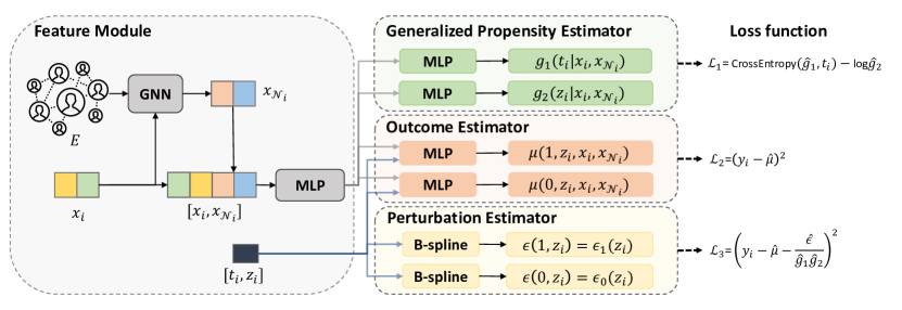
Figure 2: Model architecture of our proposed TNet. The feature module aggregates the information of covariates of unit $i$ and its neighbor. The generalized propensity estimator module aims to estimate individual propensity score and neighborhood propensity score respectively. The outcome estimator module aims to estimate potential outcomes of unit $i$. The perturbation estimator module aims to estimate $\epsilon(t,z)$ that is adapted into our estimator to achieve double robustness property.

5 How to Design DR Targeted Estimators under Interference?

In this section, we answer the question of how to design our doubly robust estimator for the whole does-response function $\psi$ under interference. We denote our model as TNet. As shown in Figure 2, our model architecture can be divided into the feature module and three estimators, generalized propensity estimator, outcome estimator, and perturbation estimator. Specifically, the perturbation estimator is to estimate $\epsilon(t,z)$ to ensure that our estimator $\hat{\psi}$ solves the EIC in Theorem 4.2. Through this alignment, our estimator gains the attribute of double robustness for any $t,z$ based on Lemma 4.3.

In the feature module, following existing work (Guo et al., 2020; Ma & Tresp, 2021; Jiang & Sun, 2022), we use Graph Convolution Networks (GCN (Defferrard et al., 2016; Kipf & Welling, 2016)) to aggregate the information of covariates of unit $i$ and its neighbors, i.e., $x_{i},x_{\mathcal{N}_{i}}$:

$$h^{neigh}_{i,1}=\sigma(\sum_{j\in\mathcal{N}_{i}}\frac{1}{\sqrt{d_{i}d_{j}}}W^{T}x_{j};\theta_{1}),$$

$$h_{i,2}=MLP_{1}(h^{neigh}_{i,1},x_{i};\theta_{2}),$$

where $\sigma(\cdot)$ is a non-linear activation function, $d_{i}$ is the degrees of unit $i$, $W$ is the weight matrix of GCN parameterized by $\theta_{1}$, and $MLP_{1}$ is a multilayer perceptron parameterized by $\theta_{2}$.

In the generalized propensity estimator module, we estimate the generalized propensity. Following (Forastiere et al., 2021), we decompose the join propensity score into individual propensity score and neighborhood propensity score, i.e., $g(T,Z|X,X_{\mathcal{N}})=g_{1}(T|X,X_{\mathcal{N}})g_{2}(Z|X,X_{\mathcal{N}})$, and estimate them respectively. Note that we can also decompose $g(T,Z|X,X_{\mathcal{N}})=g_{1}(T|X,X_{\mathcal{N}})g_{2}(Z|T,X,X_{\mathcal{N}})$ by allowing the dependence between $Z$ and $T$. The different modeling way may result in model misspecification, while our DR estimator is robust to this kind of model misspecification if our outcome model is consistent.

For binary treatment $T$, we use the sigmoid function as the last activation function to approximate $g_{1}(T|X,X_{\mathcal{N}})$:

$$g_{1}^{NN}(t_{1}|x_{i},x_{\mathcal{N}_{i}})=h_{i,3}=sigmoid(MLP_{2}(h_{i,2};\theta_{3})).$$

For continuous exposure $Z$, we use piecewise linear functions (Nie et al., 2021) to approximate $g_{2}(Z|X,X_{\mathcal{N}})$:

$$h_{i,4}=softmax(MLP_{3}(h_{i,2};\theta_{4}))\in\mathbb{R}^{B+1},$$

where we divide $[0,1]$ into $B$ grids, and estimate the conditional density $g_{2}(Z|X,X_{\mathcal{N}})$ on the $(B+1)$ grid points. Here $h_{i,4}=[h_{i,4}^{0},...,h_{i,4}^{B}]$ and $h_{i,4}^{j}$ is the estimated conditional density of $Z=\frac{j}{B}$ given $X=x_{i},X_{\mathcal{N}}=x_{\mathcal{N}_{i}}$. Estimation of conditional density at $z_{i}$ given $x_{i},x_{\mathcal{N}_{i}}$ can be obtained via linear interpolation:

$$g_{2}^{nn}(z_{i}|x_{i},x_{\mathcal{N}_{i}})=h_{i,4}^{z_{1}}+B(h_{i,4}^{z_{2}}-h_{i,4}^{z_{1}})(z_{i}-z_{1}),$$

where $z_{1}=\lfloor Bz_{i}\rfloor$ and $z_{2}=\lceil Bz_{i}\rceil$ denote the least integer greater than or equal to $Bz_{i}$ and the least integer less than or equal to $Bz_{i}$, respectively.

Then, the loss function in this module is

$$\mathcal{L}_{1}(\theta_{1},\theta_{2},\theta_{3},\theta_{4})= \Sigma_{i=1}^{n}[\alpha\text{CrossEntropy}(g_{1}^{NN}(t_{i}|x_{i},x_{\mathcal{N}_{i}}),t_{i})$$ (7)

$$-\gamma\log g_{2}^{NN}(z_{i}|x_{i},x_{\mathcal{N}_{i}})],$$

where $\alpha$ and $\gamma$ are the hyper-parameters controlling the strength of different loss functions.

In the outcome estimator module, we use two MLPs to estimate $y_{i}$ of treated and control groups respectively, i.e.,

$$\mu^{NN}(t_{i},z_{i},x_{i},x_{\mathcal{N}_{i}};\theta_{5},\theta_{6})=\left\{\begin{aligned} MLP_{3}(z_{i},h_{i,2};\theta_{5})&\quad\quad t_{i}=1\\ MLP_{4}(z_{i},h_{i,2};\theta_{6})&\quad\quad t_{i}=0\end{aligned}\right.$$

and the loss function is

$$\mathcal{L}_{2}(\theta_{1},\theta_{2},\theta_{5},\theta_{6})=\Sigma_{i=1}^{n}(y_{i}-\mu^{NN}(t_{i},z_{i},x_{i},x_{\mathcal{N}_{i}}))^{2}.$$ (8)

In the perturbation estimator module, we estimate $\epsilon$ for each pair $t_{i},z_{i}$ using spline $\{\varphi_{k}\}_{k=1}^{K_{n_{0}}}$ with with $K_{n_{0}}$ and $\{\varphi_{k}\}_{k=1}^{K_{n_{1}}}$ with $K_{n_{1}}$ basis functions:

$$\epsilon^{NN}(t_{i},z_{i})=\left\{\begin{aligned} \Sigma_{k=1}^{K_{n_{1}}}\theta_{7,k}\varphi_{k}(z_{i})&\quad\quad t_{i}=1\\ \Sigma_{k=1}^{K_{n_{0}}}\theta_{8,k}\varphi_{k}(z_{i})&\quad\quad t_{i}=0\end{aligned}\right.$$

where $\theta_{7}=\{\theta_{7,k}\}_{k=1}^{K_{n_{1}}}$ and $\theta_{8}=\{\theta_{8,k}\}_{k=1}^{K_{n_{0}}}$ are the optimized parameters.

The perturbation parameter works as the coefficient of the clever covariate $\frac{\mathds{1}_{T,Z}(t_{i},z_{i})}{g(t,z|x_{i},x_{\mathcal{N}_{i}})}$, and are obtained by the regression of the outcome $Y$. Thus, the loss function is

$$\mathcal{L}_{3}(\theta_{1},\theta_{2},\theta_{3},\theta_{4},\theta_{5},\theta_{6},\theta_{7},\theta_{8})$$ (9)

$$= \beta\Sigma_{i=1}^{n}\left[y_{i}-\left(\mu^{NN}(t_{i},z_{i},x_{i},x_{\mathcal{N}_{i}})\right.\right.$$

$$\left.\left.+\epsilon^{NN}(t_{i},z_{i})\frac{\mathds{1}_{T,Z}(t_{i},z_{i})}{g_{1}^{NN}(t_{i}|x_{i},x_{\mathcal{N}_{i}})g_{2}^{NN}(z_{i}|x_{i},x_{\mathcal{N}_{i}})}\right)\right]^{2}$$

where $\beta$ is the hyper-parameter controlling the strength of different loss functions and same as TMLE, the resulting final estimator is $\mu^{NN}(t_{i},z_{i},x_{i},x_{\mathcal{N}_{i}})+\epsilon^{NN}(t_{i},z_{i})\frac{\mathds{1}_{T,Z}(t_{i},z_{i})}{g_{1}^{NN}(t_{i}|x_{i},x_{\mathcal{N}_{i}})g_{2}^{NN}(z_{i}|x_{i},x_{\mathcal{N}_{i}})}$.

In the optimization step, inspired by the three-step TMLE estimator, we optimize our model iteratively. At each iteration, we first minimize $\mathcal{L}_{1}+\mathcal{L}_{2}$, and then minimize $\mathcal{L}_{3}$.

After training our model, our resulting estimator of the potential outcome is that, for a specified value of $t,z$ we have $\hat{y}_{i}(t,z)=\hat{\mu}(t,z,x_{i},x_{\mathcal{N}_{i}})+\frac{\hat{\epsilon}(t,z)}{\hat{g}_{1}(t|x_{i},x_{\mathcal{N}_{i}})\hat{g}_{2}(z|x_{i},x_{\mathcal{N}_{i}})}$. And thus, to infer $\hat{\tau}^{(t,z),(t^{\prime},z^{\prime})}$, the mean difference between $t,z$ and $t^{\prime},z^{\prime}$, we have

$$\hat{\tau}^{(t,z),(t^{\prime},z^{\prime})}=\Sigma_{i}^{n}\hat{y}_{i}(t,z)-\Sigma_{i}^{n}\hat{y}_{i}(t^{\prime},z^{\prime}),$$

where $n$ is the sample size.

Our estimator is a DR estimator. The key observation is, that for each pair $t,z$, the minimizer $\hat{\mu},\hat{g},\hat{\epsilon}$ of loss $\mathcal{L}$ follows

$$0 =\frac{\partial(\mathcal{L})}{\partial\epsilon}|_{\epsilon=\hat{\epsilon}}=\frac{\partial(\mathcal{L}_{1}+\mathcal{L}_{2}+\mathcal{L}_{3})}{\partial\epsilon}|_{\epsilon=\hat{\epsilon}}$$ (10)

$$=2\beta\Sigma_{i=1}^{n}\varphi(t,z,x_{i},x_{\mathcal{N}_{i}};\hat{\mu},\hat{g},\psi).$$

According to Lemma 4.3, our estimator is doubly robust: even if one of the generalized propensity estimator and outcome estimator is biased, we can still promise $\hat{\psi}$ is unbiased.

6 Analysis of the Estimator

In this section, we establish the convergence rate for our estimator using loss function $\mathcal{L}$ in Eq. 10. We find that, under some mild assumption, using our perturbation estimator theoretically helps us obtain a better estimator of $\psi$.

Theorem 6.1.

Under Assumptions 3.1, 3.2, 3.3, 3.4, and the following assumptions:

1. there exists constant $c>0$ such that for any $t\in\mathcal{T},z\in\mathcal{Z},x\in\mathcal{X},x_{\mathcal{N}}\in\mathcal{X}_{\mathcal{N}}$, and $g^{NN}\in\mathcal{Q}$, we have $\frac{1}{c}\leq g^{NN}(t,z|x,x_{\mathcal{N}})\leq c,\frac{1}{c}\leq g(t,z|x,x_{\mathcal{N}})\leq c,\lVert\mathcal{Q}\rVert_{\infty}\leq c$ and $\lVert\mu\rVert_{\infty}\leq c$.

2. $Y=\mu(T,Z,X,X_{\mathcal{N}})+V$ where $\mathbb{E}V=0,V\Vbar X,X_{\mathcal{N}},V\Vbar T,Z$ and $V$ follows sub-Gaussian distribution.

3. $g,\mu,g^{NN},\mu^{NN}$ have bounded second derivatives for any $g^{NN}\in\mathcal{Q},\mu^{NN}\in\mathcal{U}$ .

4. Either $\overline{g}=g$ or $\overline{\mu}=\mu$. And $\text{Rad}_{n}(\mathcal{Q})$, $\text{Rad}_{n}(\mathcal{U})=O(n^{-1/2})$.

5. $\mathcal{B}_{K_{n_{1}}}$, $\mathcal{B}_{K_{n_{0}}}$ equal the closed linear span of B-spline with equally spaced knots, fixed degree, and dimension $K_{n_{1}}\asymp n_{1}^{-1/6}$,$K_{n_{0}}\asymp n_{0}^{-1/6}$.

then we have

$$\lVert\hat{\phi}-\phi\rVert_{L^{2}}=O_{p}(n_{0}^{-1/3}\sqrt{\log n_{0}}+n_{1}^{-1/3}\sqrt{\log n_{1}}+r_{1}(n)r_{2}(n)),$$ (11)

where $\lVert\hat{g}-g\rVert_{\infty}=O_{p}(r_{1}(n))$ and $\lVert\hat{u}-u\rVert_{\infty}=O_{p}(r_{2}(n))$.

The required assumptions are mild and common. Assumptions 1, 3 and the first half of assumption 5 are weak and standard conditions for establishing the convergence rate of spline estimators (Huang, 2003; Huang et al., 2004; Wang et al., 2008). The second part of assumption 5, i.e., $K_{n_{1}}\asymp n_{1}^{-1/6}$, $K_{n_{0}}\asymp n_{0}^{-1/6}$, restricts the growth rate of $K_{n_{1}},K_{n_{0}}$, which is the typical assumption (Huang, 2003; Huang et al., 2004, 2002) and the different rates of $K_{n}$ are taken to achieve uniform bound. The assumption 2 bounds the tail behavior of $V$. Assumption 4 is also a very common assumption for problems with nuisance functions (Kennedy et al., 2017; Nie et al., 2020; Liu et al., 2023). Assumption 4 states that at least one of $\hat{\mu}$ and $\hat{g}$ should be consistent, which is arguably the most important, and involves the complexity of model space. Since only one of $\hat{\mu},\hat{g}$ is required to be consistent (not both), Theorem 6.1 again shows the double robustness of the proposed estimator $\hat{\psi}$.

The convergence rate given in Theorem 6.1 is a sum of two components. The first, $n_{0}^{-1/3}\sqrt{\log n_{0}}+n_{1}^{-1/3}\sqrt{\log n_{1}}$, is the rate achieved in term of $\epsilon$ using B-spline estimators. The second component, $r_{1}(n)r_{2}(n)$, is the product of the local rates of convergence of the nuisance estimators $\hat{\mu}$ and $\hat{g}$ towards their targets $\mu$ and $g$. Thus, if both estimates converge slowly, the convergence rate of $\hat{\psi}$ will also be slow. However, since the term is a product, $\hat{\psi}$ enjoys a doubly robust convergence rate. That is, when one of the nuisance estimators is misspecified, then as long as the other one is consistent ($r_{1}(n)=o(1)$ or $r_{2}(n)=o(1)$), we still have consistency ($r_{1}(n)r_{2}(n)=o(1)$). More attractively, even if we use neural networks as estimators that are consistent based on the universal approximation theorem, the estimator enjoying the double robustness property can achieve a faster convergence rate than non-doubly robust estimators whose convergence rate generally matches that of the nuisance function estimate.

7 Experiments

Table 1: Experimental results on BC(homo) Dataset. The top result is highlighted in bold, and the runner-up is underlined.

Metric	setting	effect	CFR+z	GEst	ND+z	NetEst	RRNet	NDR	TNet(w/o. $\mathcal{L}_{3}$)	TNet
$\varepsilon_{average}$	Within Sample	AME	$0.1010_{\pm 0.0678}$	$0.1512_{\pm 0.1073}$	$0.0868_{\pm 0.0757}$	$0.1257_{\pm 0.1343}$	$\underline{0.0877}_{\pm 0.0565}$	$0.5033_{\pm 0.0080}$	$0.1056_{\pm 0.0690}$	$0.0481_{\pm 0.0365}$
		ASE	$0.1956_{\pm 0.0582}$	$0.1860_{\pm 0.0225}$	$0.2140_{\pm 0.0287}$	$0.0347_{\pm 0.0169}$	$\underline{0.0227}_{\pm 0.0165}$	$0.2464_{\pm 0.0042}$	$0.1337_{\pm 0.0139}$	$0.0180_{\pm 0.0183}$
		ATE	$0.2802_{\pm 0.1814}$	$0.1342_{\pm 0.0785}$	$0.3742_{\pm 0.1041}$	$0.1229_{\pm 0.0583}$	$0.0907_{\pm 0.0662}$	$0.0284_{\pm 0.0149}$	$0.2467_{\pm 0.0520}$	$\underline{0.0533}_{\pm 0.0405}$
	Out-of Sample	AME	$0.1011_{\pm 0.0681}$	$0.1534_{\pm 0.1025}$	$0.0901_{\pm 0.0750}$	$0.1258_{\pm 0.1350}$	$0.0879_{\pm 0.0561}$	/	$0.1081_{\pm 0.0671}$	$0.0481_{\pm 0.0364}$
		ASE	$0.1969_{\pm 0.0581}$	$0.1859_{\pm 0.0228}$	$0.2127_{\pm 0.0279}$	$0.0322_{\pm 0.0173}$	$\underline{0.0225}_{\pm 0.0167}$	/	$0.1238_{\pm 0.0094}$	$0.0179_{\pm 0.0183}$
		ATE	$0.2792_{\pm 0.1826}$	$0.1298_{\pm 0.0782}$	$0.3688_{\pm 0.1040}$	$0.1238_{\pm 0.0568}$	$\underline{0.0911}_{\pm 0.0667}$	/	$0.2358_{\pm 0.0503}$	$0.0532_{\pm 0.0405}$
$\varepsilon_{individual}$	Within Sample	IME	$0.1234_{\pm 0.0580}$	$0.2021_{\pm 0.0780}$	$0.1150_{\pm 0.0642}$	$0.1411_{\pm 0.1240}$	$\underline{0.0951}_{\pm 0.0527}$	/	$0.1497_{\pm 0.0596}$	$0.0506_{\pm 0.0352}$
		ISE	$0.1974_{\pm 0.0579}$	$0.1890_{\pm 0.0217}$	$0.2155_{\pm 0.0289}$	$0.0493_{\pm 0.0163}$	$\underline{0.0304}_{\pm 0.0139}$	/	$0.1532_{\pm 0.0155}$	$0.0196_{\pm 0.0179}$
		ITE	$0.3033_{\pm 0.1562}$	$0.1848_{\pm 0.0635}$	$0.3780_{\pm 0.1031}$	$0.1278_{\pm 0.0583}$	$\underline{0.1010}_{\pm 0.0587}$	/	$0.2783_{\pm 0.0493}$	$0.0560_{\pm 0.0383}$
	Out-of Sample	IME	$0.1254_{\pm 0.0572}$	$0.2031_{\pm 0.0749}$	$0.1195_{\pm 0.0658}$	$0.1412_{\pm 0.1246}$	$\underline{0.0953}_{\pm 0.0524}$	/	$0.1487_{\pm 0.0574}$	$0.0506_{\pm 0.0351}$
		ISE	$0.1987_{\pm 0.0578}$	$0.1890_{\pm 0.0217}$	$0.2142_{\pm 0.0277}$	$0.0465_{\pm 0.0159}$	$\underline{0.0306}_{\pm 0.0144}$	/	$0.1411_{\pm 0.0105}$	$0.0195_{\pm 0.0178}$
		ITE	$0.3061_{\pm 0.1524}$	$0.1822_{\pm 0.0626}$	$0.3730_{\pm 0.1026}$	$0.1283_{\pm 0.0569}$	$\underline{0.1019}_{\pm 0.0589}$	/	$0.2612_{\pm 0.0472}$	$0.0560_{\pm 0.0380}$

In this section, we validate the proposed method TNet on two commonly used semisynthetic datasets. In detail, we verify the effectiveness of our algorithm and further evaluate the correctness of the analysis with the help of semisynthetic datasets. In particular, we aim to answer the following research questions (RQs):

• RQ1: How does the proposed method compare with the existing methods in terms of effect estimation performance?

• RQ2: How does the perturbation estimator module affect the performance of our methods?

• RQ3: Des our method stably perform well under different choices of hyperparameters?

We first introduce the experimental setup and then answer the questions above by conducting corresponding experiments. Additional results can be found in Appendix.

7.1 Datasets

It is impossible to observe the potential outcome $y_{i}(t^{\prime}_{i},z^{\prime}_{i})$ for a unit $i$ receiving $t_{i},z_{i}$. Thus, following existing works (Jiang & Sun, 2022; Guo et al., 2020; Ma et al., 2021; Cai et al., 2023), our semisynthetic datasets to evaluate our proposed method are from:

• BlogCatalog (BC) is an online community where users post blogs. In this dataset, each unit is a blogger and each edge is the social link between units. The features are bag-of-words representations of keywords in bloggers’ descriptions.

• Flickr is an online social network where users can share images and videos. In this dataset, each unit is a user and each edge is the social relationship between units. The features are the list of tags of units’ interests.

We reuse the data generation by Jiang & Sun (2022). As for the original datasets, the potential outcome is simulated by

$$\small y_{i}(t_{i},z_{i})=t_{i}+z_{i}+po_{i}+0.5\times po_{\mathcal{N}_{i}}+e_{i},$$

where $e_{i}$ is a Gaussian noise term, and $po_{i}=Sigmoid(w_{2}\times x_{i})$, and $po_{\mathcal{N}_{i}}$ is the averages of $po_{i}$. Here, $w_{2}$ is a randomly generated weight vector that mimics the causal mechanism from the features to outcomes. We denote them as BC(homo) and Flickr(homo) because the original datasets measure the homogeneous causal effects. We modify the outcome generation for heterogeneous effect estimation, as

$$\small y_{i}(t_{i},z_{i})= t_{i}+z_{i}+po_{i}+0.5\times po_{\mathcal{N}_{i}}$$

$$+t_{i}\times(po_{i}+0.5\times po_{\mathcal{N}_{i}})+e_{i},$$

which is denoted as BC(hete) and Flickr(hete) .

7.2 Baselines, Metrics

7.2.1 Baselines

We compare our methods TNet with several baselines, including neural network-based and non-neural network-based methods. We modify CFR (Johansson et al., 2021) and ND (Guo et al., 2020) by additionally inputting the exposure $z_{i}$, denoted as CFR+z and ND+z respectively. We also take baselines that are designed for effect estimation under networked interference, including GEst (Ma & Tresp, 2021), NetEst (Jiang & Sun, 2022) and RRNet (Cai et al., 2023). We use the semiparametric doubly robust estimator under network interference, named NDR (Liu et al., 2023), as one of the baselines. Since NDR is used to identify average effects on the given training data, we only report its results regarding AME, ASE, and ATE on Within Sample.

7.2.2 Metrics

In this paper, we use the Mean Absolute Error (MAE) on AME, ASE, and ATE as our metric, i.e., $\varepsilon_{average}=|\hat{\tau}-\tau|$, where $\tau$ and $\hat{\tau}$ are the average causal effect and estimated one. We also use the Rooted Precision in Estimation of Heterogeneous Effect on IME, ASE, and ITE, $\varepsilon_{individual}=\sqrt{\frac{1}{n}\Sigma_{i=1}^{n}(\hat{\tau}_{i}-\tau_{i})^{2}}$, where $\tau_{i}$ and $\hat{\tau}_{i}$ are the individual causal effect and estimated one. The mean and standard deviation of these metrics via $5$ times running are reported. Note that our main estimands are AME, ASE, and ATE in this paper.

7.3 Outperforming Existing Methods (RQ1)

As shown in Table 1, we have conducted experiments by running TNet and several baselines. Overall, TNet outperforms baselines, showing its effectiveness. Specifically, focusing on the metrics for average causal effects, i.e., AME, ASE, and ATE, compared with the neural network-based methods, TNet emerges as the top-performing solution, exhibiting not only the lowest Mean Absolute Error (MAE) but also a minimal standard deviation. This consistency signifies TNet’s effectiveness and stability. Compared with NDR, TNet still outperforms it, and the reasons might be the flexibility of our one-step learning network that shares information between two nuisance functions and the inappropriate assumptions of NDR. Turning attention to the individual causal effects, i.e., IME, ISE, and ITE, TNet consistently provides accurate estimates that align closely with the baselines. This showcases that while TNet is purposefully designed as a DR estimator for average effects, it remains a robust and highly effective estimator for individual causal effects as well.

7.4 Ablation on $\mathcal{L}_{3}$ (RQ2)

As shown in Table 1, we have conducted a comparison between the performances of TNet and TNet(w/o. $\mathcal{L}_{3}$) across two datasets. Overall, TNet outperforms TNet(w/o. $\mathcal{L}_{3}$). This result is expected, given that $\mathcal{L}_{3}$ introduces double robustness to TNet, enabling the conditional outcome model and the propensity score model to collaboratively mitigate bias as shown in Theorem 6.1. Moreover, TNet(w/o. $\mathcal{L}_{3}$) performs worse than NetEst and RRNet, because it can be seen as a ’pure’ variant of these methods without the balancing/reweighting modules in their networks.

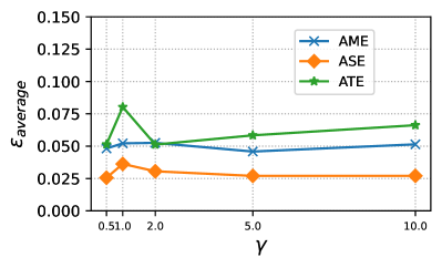
(a) $\alpha=1.0$ (on BC)

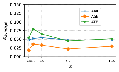
(b) $\gamma=1.0$ (on BC)

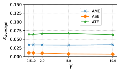
(c) $\alpha=1.0$ (on BC(hete))

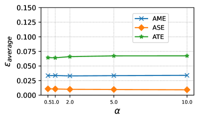
(d) $\gamma=1.0$ (on BC(hete))

Figure 3: Sensitivity analysis results on BC and BC_hete datasets.

7.5 Stability Regarding Hyperparameters (RQ3)

In Figure 3, we perform experiments with TNet using different values of hyperparameters $\alpha$ and $\gamma$. By fixing one hyperparameter and varying another one, we observe that TNet consistently achieves the MAEs of less than $0.1$ for three kinds of causal effects. Notably, when either $\alpha$ or $\gamma$ becomes excessively large, there is a slight decrease in TNet’s performance. This can be attributed to the loss imbalance caused by extremely large hyperparameters. From these findings, we can conclude that TNet exhibits robustness to variations in hyperparameter choices. Additional stability experimental results on other datasets and regarding the grid numbers $B$ can be found in Appendix.

8 Conclusion

In this work, we address the problem of how to design a targeted estimator under networked interference. Specifically, we adapt the TMLE technique to accommodate networked interference and establish the condition under which the estimator achieves double robustness. Leveraging our theoretical findings, we develop our estimator TNet, by adapting the identified condition into a targeted loss, ensuring the double robustness property of our causal effect estimator under networked interference. We provide the theoretical analysis of our design estimator, showing its advantages in terms of convergence rate. Compared with existing methods that solely model the conditional outcome or the propensity score, our estimator achieves lower bias and double robustness. Extensive experimental results verify the correctness of our theory and the effectiveness of TNet.

9 Impact Statement

This paper presents TNet whose goal is to estimate causal effects under networked interference. Our TNet could be applied to a wide range of applications, such as decision-making in marketing, and preventive measure study in epidemiology.

Appendix A Complete Definitions of Causal Effects

Due to the limited space of the main body, we give more detailed definitions of IME, ISE, and ITE, as well as AME, ASE, and ATE, in the following Appendix. Note that our main goal is to infer AME, ASE, and ATE.

Definition A.1 (Individual Main Effects (IME) ).

IME measures the difference in mean outcomes of a particular unit $x_{i}$ assigned to $T=t,Z=0$ and assigned $T=t^{\prime},Z=0$: $\tau_{i}(x_{i},x_{\mathcal{N}_{i}})^{(t,0),(t^{\prime},0)}=\mu(x_{i},x_{\mathcal{N}_{i}},t,0)-\mu(x_{i},x_{\mathcal{N}_{i}},t^{\prime},0)$.

Definition A.2 (Individual Spillover Effects (ISE) ).

ISE measures the difference in mean outcomes of a particular unit $x_{i}$ assigned to $T=0,Z=z$ and assigned $T=0,Z=z^{\prime}$: $\tau_{i}(x_{i},x_{\mathcal{N}_{i}})^{(0,z),(0,z^{\prime})}=\mu(x_{i},x_{\mathcal{N}_{i}},0,z)-\mu(x_{i},x_{\mathcal{N}_{i}},0,z^{\prime})$.

Definition A.3 (Individual Total Effects (ITE) ).

ITE measures the difference in mean outcomes of a particular unit $x_{i}$ assigned to $T=t,Z=z$ and assigned $T=t^{\prime},Z=z^{\prime}$: $\tau_{i}(x_{i},x_{\mathcal{N}_{i}})^{(t,z),(t^{\prime},z^{\prime})}=\mu(x_{i},x_{\mathcal{N}_{i}},t,z)-\mu(x_{i},x_{\mathcal{N}_{i}},t^{\prime},z^{\prime})$.

The main effects reflect the effects of changing treatment $t$ to $t^{\prime}$ of the specified unit $x_{i}$. The spillover effects reflect the effects of changing neighborhood exposure $z$ to $z^{\prime}$ of the specified unit $x_{i}$. Similarly, the total effects represent the combined effect of both main effects and spillover effects of the specified unit $x_{i}$.

Definition A.4 (Average Main Effects (AME) ).

AME measures the difference in mean outcomes between units assigned to $T=t,Z=0$ and assigned $T=t^{\prime},Z=0$: $\tau^{(t,0),(t^{\prime},0)}=\psi(t,0)-\psi(t^{\prime},0)$.

Definition A.5 (Average Spillover Effects (ASE) ).

ASE measures the difference in mean outcomes between units assigned to $T=0,Z=z$ and assigned $T=0,Z=z^{\prime}$: $\tau^{(0,z),(0,z^{\prime})}=\psi(0,z)-\psi(0,z^{\prime})$.

Definition A.6 (Average Total Effects (ATE) ).

ATE measures the difference in mean outcomes between units assigned to $T=t,Z=z$ and assigned $T=t^{\prime},Z=z^{\prime}$: $\tau^{(t,z),(t^{\prime},z^{\prime})}=\psi(t,z)-\psi(t^{\prime},z^{\prime})$.

Appendix B Additional Notations

We denote the sample size as $n$, the sample size of $t=1$ as $n_{1}$, and the sample size of $t=0$ as $n_{0}$. We denote $\mathbb{E}$ as expectation, $\mathbb{P}$ as population probability measure, $\mathbb{P}_{n}$ as the expirical measure and write $\mathbb{P}(f)=\int f(x)d\mathbb{P}(z)$, $\mathbb{P}_{n}(f)=\int f(x)d\mathbb{P}_{n}(z)$. We denote $\tau$ as Rademacher random variables, and denote Rademacher complexity of a function class $\mathcal{F}:\mathcal{X}\rightarrow\mathbb{R}$ as $\text{Rad}_{n}(\mathcal{F})=\mathbb{E}(\sup_{f\in\mathcal{F}}|\frac{1}{n}\Sigma_{i=1}^{n}\tau_{i}f(X_{i})|)$. Given two functions $f_{1},f_{2}:\mathcal{X}\rightarrow\mathbb{R}$, we define $\lVert f_{1}-f_{2}\rVert_{\infty}=\sup_{x\in\mathcal{X}}|f_{1}(x)-f_{2}(x)|$ and $\lVert f_{1}-f_{2}\rVert_{L^{2}}=(\int_{x\in\mathcal{X}}(f_{1}(x)-f_{2}(x))^{2}dx)^{1/2}$. For a function class $\mathcal{F}$, we denote $\lVert\mathcal{F}\rVert_{\infty}=\sup_{f\in\mathcal{F}}\lVert f\rVert_{\infty}$. For any function $f$ and function spaces $\mathcal{F}_{1},\mathcal{F}_{2}$, we write $\mathcal{F}_{1}+\mathcal{F}_{2}=\{f_{1}+f_{2}:f_{1}\in\mathcal{F}_{1},f_{2}\in\mathcal{F}_{2}\}$, $\mathcal{F}_{1}\mathcal{F}_{2}=\{f_{1}f_{2}:f_{1}\in\mathcal{F}_{1},f_{2}\in\mathcal{F}_{2}\}$, $f\mathcal{F}=\{fh:h\in\mathcal{F}\}$, $f\circ\mathcal{F}=\{f\circ h:h\in\mathcal{F}\}$, and $\mathcal{F}^{a}=\{f^{a}:f\in\mathcal{F}\},\forall a\in\mathbb{R}$.

Further, we denote stochastic boundedness with $O_{p}$ and convergence in probability with $o_{p}$. We denote $X_{1}\Vbar X_{2}$ as the independence between $X_{1},X_{2}$. We use $a_{n}\asymp b_{n}$ to denote both $a_{n}/b_{n}$ and $b_{n}/a_{n}$ are bounded. We use $a_{n}\lesssim b_{n}$ to denote both $a_{n}\leq Cb_{n}$ for some constant $C>0$. We use $\hat{\circ}$ to denote the minimizer of loss function, i.e., $\hat{u},\hat{g},\hat{\epsilon}$ is the minimizer of $\mathcal{L}$. We use $\overline{\circ}$ to denote a fixed function that $\hat{\circ}$ converges, e.g, $\hat{\mu}$ converges in the sense that $\lVert\hat{\mu}-\overline{\mu}\rVert_{\infty}=o_{p}(1)$. Let $\mathcal{Q},\mathcal{U}$ as the functional space in which $g^{NN},u^{NN}$ lie. We also define $\check{\epsilon}_{n}(\cdot)=\mathbb{P}[(Y-\hat{\mu}_{n})/\hat{g}_{n}|T=\cdot,Z=\cdot]/\mathbb{P}[\hat{g}_{n}^{2}|T=\cdot,Z=\cdot]$.

Appendix C Proof of Theorem 4.2

We restate the Theorem 4.2 as follows:

Theorem C.1.

For $t\in\{0,1\},z\in[0,1]$, the efficient influence curve of $\psi(t,z)$ is:

$$\varphi(t,z,X,X_{\mathcal{N}};\mu,g,\psi)\left(\frac{\mathds{1}_{T,Z}(t,z)}{g(t,z|X,X_{\mathcal{N}})}\right)\left(y-\mu(t,z,X,X_{\mathcal{N}})\right)+\mu(t,z,X,X_{\mathcal{N}})-\psi(t,z),$$ (12)

where $\mu(t,z,X,X_{\mathcal{N}}):=\mathbb{E}[Y|t,z,X,X_{\mathcal{N}}]$ and $g(t,z|X,X_{\mathcal{N}}):=\mathbb{E}[t,z|X,X_{\mathcal{N}}]$.

Our main notations and the proof structure follow (Hines et al., 2022b), which gives derivations of EIC under no interference assumption.

Proof.

Under the usual identifying assumptions, the conditional average dose-response function $\psi(t_{0},z_{0})$ can be written as:

$$\Psi(P_{0})=\psi(t_{0},z_{0})=\mathbb{E}[\mathbb{E}[Y|X,X_{\mathcal{N}},T=t_{0},Z=z_{0}]],$$ (13)

where $P_{0}$ denote the underlying true distribution, and $\Psi(P_{0})$ is a function that maps the distribution $P_{0}$ into the target parameter, potential outcome mean.

Pertubing $P_{0}$ in the direction of a point mass at $(\widetilde{x},\widetilde{x}_{\mathcal{N}},\widetilde{t},\widetilde{z},\widetilde{y})$, we have

$$\Psi(P_{\epsilon}) =\int yp_{\epsilon}(y|t_{0},z_{0},x,x_{\mathcal{N}})p_{\epsilon}(x,x_{\mathcal{N}})dydxdx_{\mathcal{N}}$$ (14)

$$=\int\frac{yp_{\epsilon}(y,t_{0},z_{0},x,x_{\mathcal{N}})p_{\epsilon}(x,x_{\mathcal{N}})}{p_{\epsilon}(t_{0},z_{0},x,x_{\mathcal{N}})}dydxdx_{\mathcal{N}},$$

where $P_{\epsilon}$ is the distribution under the parametric submodel and $p_{\epsilon}$ is the corresponding density function under the parametric submodel. To get the EIC, by the chain rule, we have:

$$\frac{\partial\Psi(P_{\epsilon})}{\partial\epsilon}\big{|}_{\epsilon=0}= \int y\left[\frac{p_{0}(x,x_{\mathcal{N}})}{p_{0}(t_{0},z_{0},x,x_{\mathcal{N}})}\frac{d}{d\epsilon}p_{\epsilon}(y,t_{0},z_{0},x,x_{\mathcal{N}})\big{|}_{\epsilon=0}+\frac{p_{0}(y,t_{0},z_{0},x,x_{\mathcal{N}})}{p_{0}(t_{0},z_{0},x,x_{\mathcal{N}})}\frac{d}{d\epsilon}p_{\epsilon}(x,x_{\mathcal{N}})\big{|}_{\epsilon=0}\right.$$ (15)

$$\left.-\frac{p_{0}(y,t_{0},z_{0},x,x_{\mathcal{N}})p_{0}(x,x_{\mathcal{N}})}{p_{0}(t_{0},z_{0},x,x_{\mathcal{N}})^{2}}\frac{d}{d\epsilon}p_{\epsilon}(t_{0},z_{0},x,x_{\mathcal{N}})\big{|}_{\epsilon=0}\right]dydxdx_{\mathcal{N}}$$

$$= \int y\frac{p_{0}(y,t_{0},z_{0},x,x_{\mathcal{N}})p_{0}(x,x_{\mathcal{N}})}{p_{0}(t_{0},z_{0},x,x_{\mathcal{N}})}\left[\frac{\frac{d}{d\epsilon}p_{\epsilon}(y,t_{0},z_{0},x,x_{\mathcal{N}})\big{|}_{\epsilon=0}}{p_{0}(y,t_{0},z_{0},x,x_{\mathcal{N}})}+\frac{\frac{d}{d\epsilon}p_{\epsilon}(x,x_{\mathcal{N}})\big{|}_{\epsilon=0}}{p_{0}(x,x_{\mathcal{N}})}\right.$$

$$\left.-\frac{\frac{d}{d\epsilon}p_{\epsilon}(t_{0},z_{0},x,x_{\mathcal{N}})\big{|}_{\epsilon=0}}{p_{0}(t_{0},z_{0},x,x_{\mathcal{N}})}\right]dydxdx_{\mathcal{N}},$$

where $p_{\epsilon}(x)$ is the density value with perturbing in the direction of a single observation $\widetilde{x}$, that is

$$p_{\epsilon}(x)=\epsilon\mathds{1}_{\widetilde{x}}(x)+(1-\epsilon)p_{0}(x),$$

and we have

$$\frac{\partial p_{\epsilon}(x)}{\partial\epsilon}=\mathds{1}_{\widetilde{x}}(x)-p_{0}(x).$$ (16)

Then, substituting Eq. 16 to Eq. 15, we have:

$$\frac{\partial\Psi(P_{\epsilon})}{\partial\epsilon}\big{|}_{\epsilon=0}$$ (17)

$$= \int y\frac{p_{0}(y,t_{0},z_{0},x,x_{\mathcal{N}})p_{0}(x,x_{\mathcal{N}})}{p_{0}(t_{0},z_{0},x,x_{\mathcal{N}})}\left[\frac{\mathds{1}_{\widetilde{x},\widetilde{x}_{\mathcal{N}},\widetilde{t},\widetilde{z},\widetilde{y}}(x,x_{\mathcal{N}},t_{0},z_{0},y)-p_{0}(x,x_{\mathcal{N}},t_{0},z_{0},y)}{p_{0}(y,t_{0},z_{0},x,x_{\mathcal{N}})}\right.$$

$$\left.+\frac{\mathds{1}_{\widetilde{x},\widetilde{x}_{\mathcal{N}}}(x,x_{\mathcal{N}})-p_{0}(x,x_{\mathcal{N}})}{p_{0}(x,x_{\mathcal{N}})}-\frac{\mathds{1}_{\widetilde{x},\widetilde{x}_{\mathcal{N}},\widetilde{t},\widetilde{z}}(x,x_{\mathcal{N}},t_{0},z_{0})-p_{0}(t_{0},z_{0},x,x_{\mathcal{N}})}{p_{0}(t_{0},z_{0},x,x_{\mathcal{N}})}\right]dydxdx_{\mathcal{N}}$$

$$= \int y\frac{p_{0}(y,t_{0},z_{0},x,x_{\mathcal{N}})p_{0}(x,x_{\mathcal{N}})}{p_{0}(t_{0},z_{0},x,x_{\mathcal{N}})}\left[\frac{\mathds{1}_{\widetilde{x},\widetilde{x}_{\mathcal{N}},\widetilde{t},\widetilde{z},\widetilde{y}}(x,x_{\mathcal{N}},t_{0},z_{0},y)}{p_{0}(y,t_{0},z_{0},x,x_{\mathcal{N}})}+\frac{\mathds{1}_{\widetilde{x},\widetilde{x}_{\mathcal{N}}}(x,x_{\mathcal{N}})}{p_{0}(x,x_{\mathcal{N}})}-\frac{\mathds{1}_{\widetilde{x},\widetilde{x}_{\mathcal{N}},\widetilde{t},\widetilde{z}}(x,x_{\mathcal{N}},t_{0},z_{0})}{p_{0}(t_{0},z_{0},x,x_{\mathcal{N}})}-1\right]dydxdx_{\mathcal{N}}$$

$$= \widetilde{y}\frac{\mathds{1}_{\widetilde{T},\widetilde{Z}}(t_{0},z_{0})p_{0}(\widetilde{x},\widetilde{x}_{\mathcal{N}})}{p_{0}(t_{0},z_{0},\widetilde{x},\widetilde{x}_{\mathcal{N}})}+\int y\frac{p_{0}(y,t_{0},z_{0},\widetilde{x},\widetilde{x}_{\mathcal{N}})}{p_{0}(t_{0},z_{0},\widetilde{x},\widetilde{x}_{\mathcal{N}})}dy-\int y\frac{\mathds{1}_{\widetilde{T},\widetilde{Z}}(t_{0},z_{0})p_{0}(y,t_{0},z_{0},\widetilde{x},\widetilde{x}_{\mathcal{N}})p_{0}(\widetilde{x},\widetilde{x}_{\mathcal{N}})}{p_{0}(t_{0},z_{0},\widetilde{x},\widetilde{x}_{\mathcal{N}})^{2}}dy$$

$$-\int y\frac{p_{0}(y,t_{0},z_{0},x,x_{\mathcal{N}})p_{0}(x,x_{\mathcal{N}})}{p_{0}(t_{0},z_{0},x,x_{\mathcal{N}})}dydxdx_{\mathcal{N}}$$

$$= \widetilde{y}\frac{\mathds{1}_{\widetilde{T},\widetilde{Z}}(t_{0},z_{0})p_{0}(\widetilde{x},\widetilde{x}_{\mathcal{N}})}{p_{0}(t_{0},z_{0},\widetilde{x},\widetilde{x}_{\mathcal{N}})}+\mathbb{E}_{p_{0}}[Y|T=t_{0},Z=z_{0},X=\widetilde{x},X_{\mathcal{N}}=\widetilde{x}_{\mathcal{N}}]$$

$$-\mathbb{E}_{p_{0}}[Y|T=t_{0},Z=z_{0},X=\widetilde{x},X_{\mathcal{N}}=\widetilde{x}_{\mathcal{N}}]\frac{\mathds{1}_{\widetilde{T},\widetilde{Z}}(t_{0},z_{0})p_{0}(\widetilde{x},\widetilde{x}_{\mathcal{N}})}{p_{0}(t_{0},z_{0},\widetilde{x},\widetilde{x}_{\mathcal{N}})}-\Psi(P_{0})$$

$$= \frac{\mathds{1}_{\widetilde{T},\widetilde{Z}}(t_{0},z_{0})p_{0}(\widetilde{x},\widetilde{x}_{\mathcal{N}})}{p_{0}(t_{0},z_{0},\widetilde{x},\widetilde{x}_{\mathcal{N}})}\left(\widetilde{y}-\mathbb{E}_{p_{0}}[Y|T=t_{0},Z=z_{0},X=\widetilde{x},X_{\mathcal{N}}=\widetilde{x}_{\mathcal{N}}]\right)+\mathbb{E}_{p_{0}}[Y|T=t_{0},Z=z_{0},X=\widetilde{x},X_{\mathcal{N}}=\widetilde{x}_{\mathcal{N}}]-\Psi(P_{0})$$

$$= \frac{\mathds{1}_{\widetilde{T},\widetilde{Z}}(t_{0},z_{0})}{g(t_{0},z_{0}|\widetilde{x},\widetilde{x}_{\mathcal{N}})}\left(\widetilde{y}-\mu(t_{0},z_{0},\widetilde{x},\widetilde{x}_{\mathcal{N}})\right)+\mu(t_{0},z_{0},\widetilde{x},\widetilde{x}_{\mathcal{N}})-\Psi(P_{0}),$$

which finishes our proof. ∎

Appendix D Proof of Lemma 4.3

We restate the Lemma 4.3 as follows:

Lemma D.1.

For $t\in\{0,1\},z\in[0,1]$, if the models $\hat{g}$ and $\hat{\mu}$ solving EIC, $\mathbb{P}\varphi(t,z,X,X_{\mathcal{N}};\hat{\mu},\hat{g},\psi)=0$, then the estimator $\hat{\psi}(t,z)$ for $\psi(t,z)$ is the doubly robust, i.e., if either $\hat{g}=g$ or $\hat{\mu}=\mu$, then $\hat{\psi}=\psi$. Further, if $\rVert\hat{g}-g\lVert_{\infty}=O_{p}(r_{1}(n))$ and $\rVert\hat{\mu}-\mu\lVert_{\infty}=O_{p}(r_{2}(n))$, we have

$$\sup_{t,z\in\mathcal{T},\mathcal{Z}}|\mathbb{P}\varphi(t,z,X,X_{\mathcal{N}};\hat{\mu},\hat{g},\psi)|=O_{p}(r_{1}(n)r_{2}(n)).$$

Proof.

Recalling that the EIC under networked interference

$$\varphi(t,z,X,X_{\mathcal{N}};m,g,\psi)=\left(\frac{\mathds{1}_{T,Z}(t,z)}{g(t,z|X,X_{\mathcal{N}})}\right)\left(Y-\mu(t,z,X,X_{\mathcal{N}})\right)+\mu(t,z,X,X_{\mathcal{N}})-\psi(t,z),$$

if an estimator solve the EIC, $\mathbb{P}\varphi(t,z,X,X_{\mathcal{N}_{i}};\hat{\mu},\hat{g},\psi)=0$, it means that

$$\mathbb{P}\varphi(t,z,X,X_{\mathcal{N}};\hat{\mu},\hat{g},\psi)= \mathbb{P}\left(\left(\frac{\mathds{1}_{T,Z}(t,z)}{\hat{g}(t,z|X,X_{\mathcal{N}}}\right)\left(Y-\hat{\mu}(t,z,X,X_{\mathcal{N}})\right)+\hat{\mu}(t,z,X,X_{\mathcal{N}})-\psi(t,z)\right)$$

$$= \mathbb{P}\left(\left(\frac{\mathds{1}_{T,Z}(t,z)}{\hat{g}(t,z|X,X_{\mathcal{N}})}\right)\left(Y-\hat{\mu}(t,z,X,X_{\mathcal{N}})\right)+\hat{\mu}(t,z,X,X_{\mathcal{N}})-\psi(t,z)\right)$$

$$= \mathbb{E}_{X,X_{N}}\left[\left(\frac{g(t,z|X,X_{\mathcal{N}})}{\hat{g}(t,z|X,X_{\mathcal{N}})}-1\right)\left(\mu(t,z,X,X_{\mathcal{N}}-\hat{\mu}(t,z,X,X_{\mathcal{N}})\right)\right].$$

From the last equation, we have the desired conclusions. ∎

Appendix E Proof of Theorem 6.1

We restate the Theorem 6.1 as follows:

Theorem E.1.

Under Assumptions 3.1, 3.2, 3.3, 3.4, and the following assumptions:

1. there exists constant $c>0$ such that for any $t\in\mathcal{T},z\in\mathcal{Z},x\in\mathcal{X},x_{\mathcal{N}}\in\mathcal{X}_{\mathcal{N}}$, and $g^{NN}\in\mathcal{Q}$, we have $\frac{1}{c}\leq g^{NN}(t,z|x,x_{\mathcal{N}})\leq c,\frac{1}{c}\leq g(t,z|x,x_{\mathcal{N}})\leq c,\lVert\mathcal{Q}\rVert_{\infty}\leq c$ and $\lVert\mu\rVert_{\infty}\leq c$.

2. $Y=\mu(T,Z,X,X_{\mathcal{N}})+V$ where $\mathbb{E}V=0,V\Vbar X,X_{\mathcal{N}},V\Vbar T,Z$ and $V$ follows sub-Gaussian distribution.

3. $g,\mu,g^{NN},\mu^{NN}$ have bounded second derivatives for any $g^{NN}\in\mathcal{Q},\mu^{NN}\in\mathcal{U}$ .

4. Either $\overline{g}=g$ or $\overline{\mu}=\mu$. And $\text{Rad}_{n}(\mathcal{Q})$, $\text{Rad}_{n}(\mathcal{U})=O(n^{-1/2})$.

5. $\mathcal{B}_{K_{n_{1}}}$, $\mathcal{B}_{K_{n_{0}}}$ equal the closed linear span of B-spline with equally spaced knots, fixed degree, and dimension $K_{n_{1}}\asymp n_{1}^{-1/6}$,$K_{n_{0}}\asymp n_{0}^{-1/6}$.

then we have

$$\lVert\hat{\phi}-\phi\rVert_{L^{2}}=O_{p}(n_{0}^{-1/3}\sqrt{\log n_{0}}+n_{1}^{-1/3}\sqrt{\log n_{1}}+r_{1}(n)r_{2}(n)),$$ (18)

where $\lVert\hat{g}-g\rVert_{\infty}=O_{p}(r_{1}(n))$ and $\lVert\hat{u}-u\rVert_{\infty}=O_{p}(r_{2}(n))$.

Proof.

First, we have

$$\left\lVert\hat{\epsilon}(\cdot)\int_{\mathcal{X}}\frac{1}{\hat{g}(\cdot|X,X_{\mathcal{N}})}d\mathbb{P}_{n}(X,X_{\mathcal{N}})-\mathbb{P}\left[\mathds{1}_{\cdot}(T,Z)\frac{Y-\hat{\mu}(T,Z,X,X_{\mathcal{N}})}{\hat{g}(T,Z|X,X_{\mathcal{N}})}\right]\right\rVert_{L^{2}}$$ (19)

$$= \left\lVert\hat{\epsilon}(\cdot)\int_{\mathcal{X}}\frac{1}{\hat{g}(\cdot|X,X_{\mathcal{N}})}d\mathbb{P}_{n}(X,X_{\mathcal{N}})-g(\cdot)\mathbb{P}\left(\frac{Y-\hat{\mu}_{n}(T,Z,X,X_{\mathcal{N}})}{\hat{g}_{n}(T,Z|X,X_{\mathcal{N}})}|T=\cdot,Z=\cdot\right)\right\rVert_{L^{2}}$$

$$\leq \left\lVert(\hat{\epsilon}(\cdot)-\check{\epsilon}(\cdot))\int_{\mathcal{X}}\frac{1}{\hat{g}(\cdot|X,X_{\mathcal{N}})}d\mathbb{P}_{n}(X,X_{\mathcal{N}})\right\rVert_{L^{2}}+\left\lVert\check{\epsilon}(\cdot)\left(\int_{\mathcal{X}}\frac{1}{\hat{g}(\cdot|X,X_{\mathcal{N}})}d\mathbb{P}_{n}(X,X_{\mathcal{N}})-g(\cdot)\mathbb{P}\left(\frac{1}{\hat{g}^{2}(\cdot|X,X_{\mathcal{N}})}|T=\cdot,Z=\cdot\right)\right)\right\rVert_{L^{2}}$$

$$\lesssim \left\lVert(\hat{\epsilon}-\check{\epsilon})\right\rVert_{L^{2}}+\left\lVert\check{\epsilon}(\cdot)\left(\int_{\mathcal{X}}\frac{1}{\hat{g}(\cdot|X,X_{\mathcal{N}})}d(\mathbb{P}_{n}-\mathbb{P})(X,X_{\mathcal{N}})\right)+\check{\epsilon}(\cdot)\left(\int_{\mathcal{X}}\frac{1}{\hat{g}(\cdot|X,X_{\mathcal{N}})}d\mathbb{P}(X,X_{\mathcal{N}})-g(\cdot)\mathbb{P}\left(\frac{1}{\hat{g}^{2}(\cdot|X,X_{\mathcal{N}})}|T=\cdot,Z=\cdot\right)\right)\right\rVert_{L^{2}}$$

$$\lesssim \left\lVert(\hat{\epsilon}-\check{\epsilon})\right\rVert_{L^{2}}+\left\lVert\check{\epsilon}(\cdot)\left(\int_{\mathcal{X}}\frac{1}{\hat{g}(\cdot|X,X_{\mathcal{N}})}d(\mathbb{P}_{n}-\mathbb{P})(X,X_{\mathcal{N}})\right)\right\rVert_{L^{2}}$$

$$+\left\lVert\mathbb{P}\left(\frac{\mu(T,Z,X,X_{\mathcal{N}})-\hat{\mu}_{n}(T,Z,X,X_{\mathcal{N}})}{\hat{g}_{n}(T,Z|X,X_{\mathcal{N}})}|T=\cdot,Z=\cdot\right)\int_{\mathcal{X}}\frac{\hat{g}(\cdot|X,X_{\mathcal{N}})-g(\cdot|X,X_{\mathcal{N}})}{\hat{g}(\cdot|X,X_{\mathcal{N}})}\frac{1}{\hat{g}(\cdot|X,X_{\mathcal{N}})}d\mathbb{P}(X,X_{\mathcal{N}})\right\rVert_{L^{2}}$$

$$\overset{(a)}{=} O_{p}(n_{0}^{-1/3}\sqrt{\log n_{0}}+n_{1}^{-1/3}\sqrt{\log n_{1}}+r_{1}(n)r_{2}(n)),$$

where Eq.(a) is based on Lemma F.1 in next Section, i.e., $\left\lVert\hat{\epsilon}_{n}-\check{\epsilon}_{n}\right\lVert=O_{p}(n_{0}^{-1/3}\sqrt{\log n_{0}}+n_{1}^{-1/3}\sqrt{\log n_{1}})$.

From generalization bound and condition 4, we have

$$\sup_{t,z\in\mathcal{T},\mathcal{Z}}\left|\frac{1}{n}\Sigma_{i=1}^{n}\hat{\mu}_{n}(t,z,x_{i},x_{\mathcal{N}_{i}})-\mathbb{P}\hat{\mu}_{n}(t,z,X,X_{\mathcal{N}})\right|=O_{p}(n^{-1/2}).$$

Thus,

$$\left\lVert\frac{1}{n}\Sigma_{i=1}^{n}\hat{\mu}_{n}(\cdot,x_{i},x_{\mathcal{N}_{i}})-\mathbb{P}\hat{\mu}_{n}(\cdot,X,X_{\mathcal{N}})\right\lVert_{L^{2}}=O_{p}(n^{-1/2}).$$ (20)

From Lemma D.1, if $\rVert\hat{g}-g\lVert_{\infty}=O_{p}(r_{1}(n))$ and $\rVert\hat{\mu}-\mu\lVert_{\infty}=O_{p}(r_{2}(n))$, we have

$$\sup_{t,z\in\mathcal{T},\mathcal{Z}}\left|\mathbb{P}\left[\left(\frac{\mathds{1}_{T,Z}(t,z)}{\hat{g}(t,z|X,X_{\mathcal{N}}}\right)\left(Y-\hat{\mu}(t,z,X,X_{\mathcal{N}})\right)+\hat{\mu}(t,z,X,X_{\mathcal{N}})\right]-\psi(t,z)\right|=O_{p}(r_{1}(n)r_{2}(n)).$$ (21)

Based on Eq. 19, 20, and 21, using triangle inequality, we have

$$\left\lVert\hat{\epsilon}(\cdot)\int_{\mathcal{X}}\frac{1}{\hat{g}(\cdot|X,X_{\mathcal{N}})}d\mathbb{P}_{n}(X,X_{\mathcal{N}})+\frac{1}{n}\Sigma_{i=1}^{n}\hat{\mu}_{n}(\cdot,x_{i},x_{\mathcal{N}_{i}})-\psi(\cdot)\right\lVert_{L^{2}}=O_{p}(n_{0}^{-1/3}\sqrt{\log n_{0}}+n_{1}^{-1/3}\sqrt{\log n_{1}}+r_{1}(n)r_{2}(n)).$$

By setting

$$\hat{\psi}(t,z)=\hat{\epsilon}(t,z)\int_{\mathcal{X}}\frac{1}{\hat{g}(t,z|X,X_{\mathcal{N}})}d\mathbb{P}_{n}(X,X_{\mathcal{N}})+\frac{1}{n}\Sigma_{i=1}^{n}\hat{\mu}_{n}(t,z,x_{i},x_{\mathcal{N}_{i}})=\frac{1}{n}\Sigma_{i=1}^{n}\left(\hat{\mu}_{n}(t,z,x_{i},x_{\mathcal{N}_{i}})+\frac{\hat{\epsilon}(t,z)}{\hat{g}(t,z|x_{i},x_{\mathcal{N}_{i}})}\right)$$

we have

$$\left\lVert\hat{\psi}-\psi\right\lVert_{L^{2}}=O_{p}(n_{0}^{-1/3}\sqrt{\log n_{0}}+n_{1}^{-1/3}\sqrt{\log n_{1}}+r_{1}(n)r_{2}(n)).$$

∎

Appendix F Convergence rate of $\hat{\epsilon}_{n}$

Lemma F.1.

Under assumptions in Theorem 3, we have

$$\left\lVert\hat{\epsilon}_{n}-\check{\epsilon}_{n}\right\lVert_{L^{2}}=O_{p}(n_{0}^{-1/3}\sqrt{\log n_{0}}+n_{1}^{-1/3}\sqrt{\log n_{1}})$$

Our proof structure follows Huang et al. (2004) and Nie et al. (2020).

Proof.

Our estimator $\hat{\epsilon}_{n}$ consists of two B-spline estimators, denoted as $\hat{\epsilon}_{1n}$ for the treated group and $\hat{\epsilon}_{0n}$ for the control group. We have

$$\left\lVert\hat{\epsilon}_{n}-\check{\epsilon}_{n}\right\lVert_{L^{2}}\leq\left\lVert\hat{\epsilon}_{1n}-\check{\epsilon}_{1n}\right\lVert_{L^{2}}+\left\lVert\hat{\epsilon}_{0n}-\check{\epsilon}_{0n}\right\lVert_{L^{2}}$$

We then prove that $\left\lVert\hat{\epsilon}_{1n}-\check{\epsilon}_{1n}\right\lVert_{L^{2}}=O_{p}(n_{1}^{-1/3}\sqrt{\log n_{1}})$ and it is similar for $\hat{\epsilon}_{0n}$, and thus we will get the desired conclusion. We skip the proof regarding $\hat{\epsilon}_{0n}$.

As denoted in the main text, $\hat{\epsilon}_{1n}=\Sigma_{k=1}^{K_{n_{1}}}\theta_{7,k}\varphi_{k}(z)$. To simplify notation and with some slight abuse of notation, we drop the index $7$ under $\hat{\theta}_{7,k}$, i.e., $\hat{\epsilon}_{1n}=\Sigma_{k=1}^{K_{n_{1}}}\hat{\theta}_{k}\varphi_{k}(z)=(\boldsymbol{\varphi}^{K_{n_{1}}}(z))^{T}\hat{\boldsymbol{\theta}}$ where $\boldsymbol{\varphi}^{K_{n_{1}}}(z)=(\varphi_{1}(z),\varphi_{2}(z),...,\varphi_{K_{n}1}(z))^{T}\in\mathbb{R}^{K_{n1}}$ and $\boldsymbol{B}_{n1}=(\varphi^{K_{n_{1}}}(z_{1}),\varphi^{K_{n_{1}}}(z_{2}),...,\varphi^{K_{n_{1}}}(z_{n1}))^{T}\in\mathbb{R}^{n_{1}\times{K_{n_{1}}}}$. Here, we define

$$\Pi_{n1}=\text{diag}(\hat{g}_{n}(1,z_{1}|x_{1},x_{\mathcal{N}_{1}}),\hat{g}_{n}(1,z_{2}|x_{2},x_{\mathcal{N}_{2}}),...,\hat{g}_{n}(1,z_{n1}|x_{n1},x_{\mathcal{N}_{n1}})),$$

$$\tilde{\Pi}_{n1}=\text{diag}\left([\mathbb{P}(\hat{g}_{n}^{2}(1,Z|X,X_{\mathcal{N}})|Z=z_{1})]^{-1/2},[\mathbb{P}(\hat{g}_{n}^{2}(1,Z|X,X_{\mathcal{N}})|Z=z_{2})]^{-1/2},...,[\mathbb{P}(\hat{g}_{n}^{2}(1,Z|X,X_{\mathcal{N}})|Z=z_{n1})]^{-1/2}\right),$$

$$\boldsymbol{W}_{n1}=(w_{1},w_{2},...,w_{n1})^{T}\in\mathbb{R}^{n1}\quad\text{where}\quad w_{i}=\frac{y_{i}-\hat{\mu}_{n}(1,z_{i},x_{i},x_{\mathcal{N}_{i}})}{\hat{g}_{n}(1,z_{i}|x_{i},x_{\mathcal{N}_{i}})},$$

$$\tilde{\boldsymbol{W}}_{n1}=(\tilde{w}_{1},\tilde{w}_{2},...,\tilde{w}_{n1})^{T}\in\mathbb{R}^{n1}\quad\text{where}\quad\tilde{w}_{i}=\mathbb{P}\left(\frac{Y-\hat{\mu}_{n}(1,Z,X,X_{\mathcal{N}})}{\hat{g}_{n}(1,Z|X,X_{\mathcal{N}})}|Z=z_{i}\right).$$

Then,

$$\hat{\boldsymbol{\theta}}=(B_{n1}^{T}\Pi_{n1}^{-2}B_{n1})^{-1}B_{n1}^{T}W_{n1}$$

$$\tilde{\boldsymbol{\theta}}=(B_{n1}^{T}\Pi_{n1}^{-2}B_{n1})^{-1}B_{n1}^{T}\Pi_{n1}^{-2}\tilde{\Pi}_{n1}^{2}\tilde{W}_{n1}$$

We decompose $\leq\left\lVert\hat{\epsilon}_{1n}-\check{\epsilon}_{1n}\right\lVert_{L^{2}}$ as follows:

$$\left\lVert\hat{\epsilon}_{1n}-\check{\epsilon}_{1n}\right\lVert_{L^{2}}\leq\left\lVert\check{\epsilon}_{1n}-\tilde{\epsilon}_{1n}\right\lVert_{L^{2}}+\left\lVert\hat{\epsilon}_{1n}-\tilde{\epsilon}_{1n}\right\lVert_{L^{2}},$$ (22)

where $\tilde{\epsilon}_{1n}=(\boldsymbol{\varphi}^{K_{n_{1}}}(z))^{T}\tilde{\boldsymbol{\theta}}$. The first term $\left\lVert\check{\epsilon}_{1n}-\tilde{\epsilon}_{1n}\right\lVert_{L^{2}}$ is the bias term and the second term $\left\lVert\hat{\epsilon}_{1n}-\tilde{\epsilon}_{1n}\right\lVert_{L^{2}}$ is the variance term. We next bound on them.

Bound on bias term

Let $\check{\boldsymbol{\theta}}\in\mathbb{R}^{K_{n1}}$ be such that $\left\lVert\check{\boldsymbol{\theta}}^{T}\boldsymbol{\varphi}^{K_{n1}}-\check{\epsilon}_{1n}\right\lVert_{\infty}=\inf_{f\in\mathcal{B}_{K_{n1}}}\left\lVert f-\check{\epsilon}_{1n}\right\lVert_{\infty}$ , then we have

$$\left\lVert\check{\epsilon}_{1n}-\tilde{\epsilon}_{1n}\right\lVert_{L^{2}} =\left\lVert\check{\epsilon}_{1n}-\check{\boldsymbol{\theta}}^{T}\boldsymbol{\varphi}^{K_{n1}}+\check{\boldsymbol{\theta}}^{T}\boldsymbol{\varphi}^{K_{n1}}-\tilde{\epsilon}_{1n}\right\lVert_{L^{2}}$$

$$\leq\left\lVert\check{\epsilon}_{1n}-\check{\boldsymbol{\theta}}^{T}\boldsymbol{\varphi}^{K_{n1}}\right\lVert_{L^{2}}+\left\lVert\check{\boldsymbol{\theta}}^{T}\boldsymbol{\varphi}^{K_{n1}}-\tilde{\epsilon}_{1n}\right\lVert_{L^{2}}.$$

The first term can be bounded based on the definition of ${\boldsymbol{\theta}}$ and the properties of B-spline space:

$$\left\lVert\check{\epsilon}_{1n}-\check{\boldsymbol{\theta}}^{T}\boldsymbol{\varphi}^{K_{n1}}\right\lVert_{L^{2}}=O_{p}(\rho_{n1}),$$

where $\rho_{n1}=\inf_{f\in\text{Span}\{\boldsymbol{\varphi}^{K_{n1}}\}\sup_{z\in\mathcal{Z}}}|\check{\epsilon}_{1n}(z)-f(z)|$, and under Assumption 3 in Theorem E.1, we have $\rho_{n1}=O(K_{n1}^{-2})$ (Theorem 6.27 in Schumaker (2007)). Also the second can be bounded:

$$\left\lVert\check{\boldsymbol{\theta}}^{T}\boldsymbol{\varphi}^{K_{n1}}-\tilde{\epsilon}_{1n}\right\lVert_{L^{2}}\overset{a}{\asymp}\frac{\left\lVert\check{\boldsymbol{\theta}}-\tilde{\boldsymbol{\theta}}\right\lVert_{2}}{\sqrt{K_{n1}}}=\frac{\left\lVert(B_{n1}^{T}\Pi_{n1}^{-2}B_{n1})^{-1}B_{n1}^{T}\Pi_{n1}^{-2}(B_{n1}\check{\boldsymbol{\theta}}-\tilde{\Pi}_{n1}^{2}\tilde{W}_{n1})\right\lVert_{2}}{\sqrt{K_{n1}}}$$ (23)

where (a) follows the properties of B-spline basis functions. Then using SVD decomposition, we have $B_{n1}=U\Lambda V^{T}$ where $U\in\mathcal{R}^{n1\times n1},\Lambda\in\mathcal{R}^{n1\times K_{n1}},V\in\mathcal{R}^{K_{n1}\times K_{n1}}$. Then all diagonal elements of $\frac{K_{n1}}{n_{1}}\Lambda^{T}\Lambda$ fall between $M_{1}$ and $M_{2}$ where $M_{1},M_{2}$ are positive constants and $\frac{K_{n1}}{n_{1}}\Lambda^{T}\Lambda$ is invertible (Lemma A.3 in Huang et al. (2004)). Since the eigenvalues of $\frac{K_{n1}}{n_{1}}B_{n1}^{T}\Pi_{n1}^{-2}B_{n1}$ are the diagonal elements of $\frac{K_{n1}}{n_{1}}\Lambda^{T}\Lambda$ and $\hat{g}_{n}$ are bounded, we have that all the eigenvalues of $\frac{K_{n1}}{n_{1}}B_{n1}^{T}\Pi_{n1}^{-2}B_{n1}$ fall between $M_{1}$ and $M_{2}$ where $M_{1},M_{2}$ are some positive constants and $\frac{K_{n1}}{n_{1}}B_{n1}^{T}\Pi_{n1}^{-2}B_{n1}$ is also invertible. Then Eq. 23 can be written:

$$\left\lVert\check{\boldsymbol{\theta}}^{T}\boldsymbol{\varphi}^{K_{n1}}-\tilde{\epsilon}_{1n}\right\lVert_{L^{2}} \asymp\frac{\left\lVert(B_{n1}^{T}\Pi_{n1}^{-2}B_{n1})^{-1}B_{n1}^{T}\Pi_{n1}^{-2}(B_{n1}\check{\boldsymbol{\theta}}-\tilde{\Pi}_{n1}^{2}\tilde{W}_{n1})\right\lVert_{2}}{\sqrt{K_{n1}}}$$ (24)

$$\asymp\frac{K_{n1}}{n_{1}}\frac{\left\lVert B_{n1}^{T}\Pi_{n1}^{-2}(B_{n1}\check{\boldsymbol{\theta}}-\tilde{\Pi}_{n1}^{2}\tilde{W}_{n1})\right\lVert_{2}}{\sqrt{K_{n1}}}$$

$$=\frac{\sqrt{K_{n1}}}{n_{1}}\left\lVert B_{n1}^{T}\Pi_{n1}^{-2}(B_{n1}\check{\boldsymbol{\theta}}-\tilde{\Pi}_{n1}^{2}\tilde{W}_{n1})\right\lVert_{2}$$

$$\overset{b}{\asymp}\frac{\sqrt{K_{n1}}}{n_{1}}\sqrt{\mathbf{1}^{T}\Pi_{n1}^{-2}B_{n1}^{T}B_{n1}\Pi_{n1}^{-2}\mathbf{1}}\rho_{n1}$$

$$\asymp\frac{\sqrt{K_{n1}}}{n_{1}}\sqrt{\Sigma_{k=1}^{K_{n1}}\left(\Sigma_{i=1}^{n_{1}}\frac{\varphi_{k}(z_{i})}{\hat{g}_{n}(1,z_{i}|x_{i},\mathcal{N}_{i})}\right)^{2}}\rho_{n1}$$

$$\asymp\sqrt{K_{n1}}\sqrt{\Sigma_{k=1}^{K_{n1}}\left(\Sigma_{i=1}^{n_{1}}\frac{1}{n_{1}}\varphi_{k}(z_{i})\right)^{2}}\rho_{n1},$$

where (b) is based on the properties of B-spline space $\left\lVert B_{n1}\check{\boldsymbol{\theta}}-\tilde{\Pi}_{n1}^{2}\tilde{W}_{n1}\right\lVert_{\infty}=O_{p}(\rho_{n1})$ since $\left(\check{\epsilon}_{1n}(z_{1}),\check{\epsilon}_{1n}(z_{2}),...,\check{\epsilon}_{1n}(z_{n_{1}})\right)^{T}=\tilde{\Pi}_{n1}^{2}\tilde{W}_{n1}$. Following Lemma A.6 in Huang et al. (2004), for any $a>[\mathbb{E}\varphi_{k}(Z)]^{2}K_{n1}$, we have

$$\text{Prob}\left(\Sigma_{k=1}^{K_{n1}}\left(\Sigma_{i=1}^{n_{1}}\frac{1}{n_{1}}\varphi_{k}(z_{i})\right)^{2}\right) \overset{a}{\leq}\Sigma_{k=1}^{K_{n1}}\text{Prob}\left(\left|\Sigma_{i=1}^{n_{1}}\frac{1}{n_{1}}\varphi_{k}(z_{i})\right|>\sqrt{\frac{a}{K_{n1}}}\right)$$

$$\leq\Sigma_{k=1}^{K_{n1}}\text{Prob}\left(\left|\Sigma_{i=1}^{n_{1}}\frac{1}{n_{1}}\varphi_{k}(z_{i})-\mathbb{E}\varphi_{k}(Z)\right|+\left|\mathbb{E}\varphi_{k}(Z)\right|>\sqrt{\frac{a}{K_{n1}}}\right)$$

$$\leq\Sigma_{k=1}^{K_{n1}}\text{Prob}\left(\left|\Sigma_{i=1}^{n_{1}}\frac{1}{n_{1}}\varphi_{k}(z_{i})-\mathbb{E}\varphi_{k}(Z)\right|>\sqrt{\frac{a}{K_{n1}}}-\left|\mathbb{E}\varphi_{k}(Z)\right|\right)$$

$$\overset{b}{\leq}2K_{n1}\exp\left\{-2n\left(\sqrt{\frac{a}{K_{n1}}}-\left|\mathbb{E}\varphi_{k}(Z)\right|\right)^{2}\right\},$$

where (a) uses union bound and (b) follows Hoeffding’s Inequality for bounded random variables. Since $\mathbb{E}\varphi_{k}(Z)\asymp 1/K_{n1}$, we pick $a=2[\mathbb{E}\varphi_{k}(Z)]^{2}K_{n1}\asymp 1/K_{n1}$ and then $\Sigma_{k=1}^{K_{n1}}\left(\Sigma_{i=1}^{n_{1}}\frac{1}{n_{1}}\varphi_{k}(z_{i})\right)^{2}=O_{p}(1/K_{n1})$. Taking it into 24, we have

$$\left\lVert\check{\boldsymbol{\theta}}^{T}\boldsymbol{\varphi}^{K_{n1}}-\tilde{\epsilon}_{1n}\right\lVert_{L^{2}}=O_{p}(\rho_{n1}).$$

Again, $\rho_{n1}=O(K_{n1}^{-2})$ under Assumptions in Theorem E.1.

Hence, we can conclude that the bias term is bounded:

$$\left\lVert\check{\epsilon}_{1n}-\tilde{\epsilon}_{1n}\right\lVert_{L^{2}}=O_{p}(\rho_{n1}).$$ (25)

Bound on variance term

Based on the properties of B-spline space, we first have

$$\left\lVert\hat{\epsilon}_{1n}-\tilde{\epsilon}_{1n}\right\lVert_{L^{2}}\lesssim\frac{\left\lVert\hat{\boldsymbol{\theta}}-\tilde{\boldsymbol{\theta}}\right\lVert_{2}}{\sqrt{K_{n1}}}.$$ (26)

Then,

$$\left\lVert\hat{\boldsymbol{\theta}}-\tilde{\boldsymbol{\theta}}\right\lVert_{2}= \left\lVert(B_{n1}^{T}\Pi_{n1}^{-2}B_{n1})^{-1}B_{n1}^{T}(\boldsymbol{W}_{n1}-\Pi_{n1}^{-2}\tilde{\Pi}_{n1}^{2}\tilde{\boldsymbol{W}}_{n1})\right\lVert_{2}$$ (27)

$$= \left\lVert(B_{n1}^{T}\Pi_{n1}^{-2}B_{n1})^{-1}B_{n1}^{T}(\boldsymbol{W}_{n1}-\tilde{\boldsymbol{W}}_{n1}+\tilde{\boldsymbol{W}}_{n1}-\Pi_{n1}^{-2}\tilde{\Pi}_{n1}^{2}\tilde{\boldsymbol{W}}_{n1})\right\lVert_{2}$$

$$\leq \left\lVert(B_{n1}^{T}\Pi_{n1}^{-2}B_{n1})^{-1}B_{n1}^{T}(\boldsymbol{W}_{n1}-\tilde{\boldsymbol{W}}_{n1})\right\lVert_{2}+\left\lVert(B_{n1}^{T}\Pi_{n1}^{-2}B_{n1})^{-1}B_{n1}^{T}(\tilde{\boldsymbol{W}}_{n1}-\Pi_{n1}^{-2}\tilde{\Pi}_{n1}^{2}\tilde{\boldsymbol{W}}_{n1})\right\lVert_{2}.$$

We first consider the first term. Denote $\boldsymbol{\delta}=(\delta_{1},...,\delta_{n_{1}}):=\boldsymbol{W}_{n1}-\tilde{\boldsymbol{W}}_{n1}$, we have:

$$\left\lVert(B_{n1}^{T}\Pi_{n1}^{-2}B_{n1})^{-1}B_{n1}^{T}(\boldsymbol{W}_{n1}-\tilde{\boldsymbol{W}}_{n1})\right\lVert_{2}^{2} =\boldsymbol{\delta}^{T}B_{n1}(B_{n1}^{T}\Pi_{n1}^{-2}B_{n1})^{-2}B_{n1}^{T}\boldsymbol{\delta}$$ (28)

$$\asymp\frac{K_{n1}^{2}}{n^{2}}\boldsymbol{\delta}^{T}B_{n1}B_{n1}^{T}\boldsymbol{\delta}$$

$$=\frac{K_{n1}^{2}}{n^{2}}\Sigma_{k=1}^{K_{n1}}\left(\Sigma_{i=1}^{n_{1}}\varphi_{k}(z_{i})\delta_{i}\right)^{2}$$

$$\leq K_{n1}^{2}\Sigma_{k=1}^{K_{n1}}\sup_{\hat{g},\hat{\mu}}\left(\frac{1}{n}\Sigma_{i=1}^{n_{1}}\varphi_{k}(z_{i})\delta_{i}\right)^{2}.$$

By definition, we rewrite $\delta_{i}$ as

$$\delta_{i}=\underbrace{\frac{\mu(1,z_{i},x_{i},x_{\mathcal{N}_{i}})-\hat{\mu}_{n}(1,z_{i},x_{i},x_{\mathcal{N}_{i}})}{\hat{g}(1,z_{i}|x_{i},x_{\mathcal{N}_{i}}))}-\mathbb{P}\left(\frac{\mu(1,Z,X,X_{\mathcal{N}})-\hat{\mu}_{n}(1,Z,X,X_{\mathcal{N}})}{\hat{g}(1,Z|X,X_{\mathcal{N}}))}|Z=z_{i}\right)}_{u_{i}}+\underbrace{\frac{v_{i}}{\hat{g}(1,z_{i}|x,x_{\mathcal{N}_{i}}))}}_{\tilde{v}_{i}},$$

where under Assumption 2 in Theorem E.1, $\mathbb{E}(\tilde{v}_{i}|z_{i},x_{i},x_{\mathcal{N}_{i}})=0$ and also $\mathbb{E}(u_{i}|z_{i})=0$. Thus, from union bound we have

$$\text{Prob}\left(\Sigma_{k=1}^{K_{n1}}\sup_{\hat{g},\hat{\mu}}\left(\frac{1}{n}\Sigma_{i=1}^{n_{1}}\varphi_{k}(z_{i})\delta_{i}\right)^{2}>a\right)$$ (29)

$$\leq \Sigma_{k=1}^{K_{n1}}\text{Prob}\left(\sup_{\hat{g},\hat{\mu}}\left(\frac{1}{n}\Sigma_{i=1}^{n_{1}}\varphi_{k}(z_{i})\delta_{i}\right)^{2}>\frac{a}{K_{n1}}\right)$$

$$= \Sigma_{k=1}^{K_{n1}}\text{Prob}\left(\sup_{\hat{g},\hat{\mu}}\left|\frac{1}{n}\Sigma_{i=1}^{n_{1}}\varphi_{k}(z_{i})\delta_{i}\right|>\sqrt{\frac{a}{K_{n1}}}\right)$$

$$= \Sigma_{k=1}^{K_{n1}}\text{Prob}\left(\sup_{\hat{g},\hat{\mu}}\left|\frac{1}{n}\Sigma_{i=1}^{n_{1}}\varphi_{k}(z_{i})(u_{i}+\tilde{v}_{i})\right|>\sqrt{\frac{a}{K_{n1}}}\right)$$

$$= \Sigma_{k=1}^{K_{n1}}\text{Prob}\left(\sup_{\hat{g},\hat{\mu}}\left|\frac{1}{n}\Sigma_{i=1}^{n_{1}}\varphi_{k}(z_{i})u_{i}\right|>\frac{1}{2}\sqrt{\frac{a}{K_{n1}}}\right)+\Sigma_{k=1}^{K_{n1}}\text{Prob}\left(\sup_{\hat{g},\hat{\mu}}\left|\frac{1}{n}\Sigma_{i=1}^{n_{1}}\varphi_{k}(z_{i})\tilde{v}_{i}\right|>\frac{1}{2}\sqrt{\frac{a}{K_{n1}}}\right)$$

Based on

$$\text{Rad}_{n}(\varphi_{k}(\mathcal{Q}+\mu)\mathcal{U}^{-1})$$

$$\overset{a}{\leq} \frac{1}{2}(\left\lVert\varphi_{k}\right\rVert_{\infty}+\left\lVert(\mathcal{Q}+\mu)\mathcal{U}^{-1}\varphi_{k}\right\rVert_{\infty})(\text{Rad}_{n}(\varphi_{k})+\text{Rad}_{n}((\mathcal{Q}+\mu)\mathcal{U}^{-1}))$$

$$\overset{a}{\leq} \frac{1}{2}(\left\lVert\varphi_{k}\right\rVert_{\infty}+\left\lVert(\mathcal{Q}+\mu)\mathcal{U}^{-1}\varphi_{k}\right\rVert_{\infty})(\text{Rad}_{n}(\varphi_{k})+\frac{1}{2}(\left\lVert\mathcal{Q}\right\rVert_{\infty}+\left\lVert\mathcal{U}^{-1}\varphi_{k}\right\rVert_{\infty})(\text{Rad}_{n}(\mathcal{Q})+\max(\frac{c^{2}}{2},\frac{2}{(c-1/c)^{2}})\text{Rad}_{n}(\mathcal{U}-\frac{1}{2c})+\frac{2c}{n_{1}})$$

$$= O(n_{1}^{1/2}),$$

where (a) is based on Lemma 5 in Nie et al. (2020), and (b) is based on Lemma 5 in Nie et al. (2020) and Theorem 12 in (Bartlett & Mendelson, 2002) by plugging $h:x\mapsto\frac{1}{x-1/2c}+2c$, then we can bound the first term in 29:

$$\text{Prob}\left(\sup_{\hat{g},\hat{\mu}}\left|\frac{1}{n}\Sigma_{i=1}^{n_{1}}\varphi_{k}(z_{i})u_{i}\right|>\frac{1}{2}\sqrt{\frac{a}{K_{n1}}}\right)$$ (30)

$$\overset{a}{\lesssim} \frac{\mathbb{E}(\sup_{\hat{g},\hat{\mu}}\left|\frac{1}{n}\Sigma_{i=1}^{n_{1}}\varphi_{k}(z_{i})u_{i}\right|)}{\frac{1}{2}\sqrt{\frac{a}{K_{n1}}}}$$

$$\overset{b}{\asymp} \sqrt{\frac{K_{n1}}{an_{1}}},$$

where (a) follows Markov Inequality and (b) follows the definition of Rademacher complexity.

Then we bound the second term in 29 using union bound: for any $M_{n1}>0$,

$$\text{Prob}\left(\sup_{\hat{g},\hat{\mu}}\left|\frac{1}{n}\Sigma_{i=1}^{n_{1}}\varphi_{k}(z_{i})\tilde{v}_{i}\right|>\frac{1}{2}\sqrt{\frac{a}{K_{n1}}}\right)$$ (31)

$$\leq \text{Prob}\left(\sup_{\hat{g},\hat{\mu}}\left|\frac{1}{n}\Sigma_{i=1}^{n_{1}}\varphi_{k}(z_{i})\tilde{v}_{i}\mathds{1}(|v_{i}|>M_{n1})\right|>\frac{1}{4}\sqrt{\frac{a}{K_{n1}}}\right)+\text{Prob}\left(\sup_{\hat{g},\hat{\mu}}\left|\frac{1}{n}\Sigma_{i=1}^{n_{1}}\varphi_{k}(z_{i})\tilde{v}_{i}\mathds{1}(|v_{i}|\leq M_{n1})\right|>\frac{1}{4}\sqrt{\frac{a}{K_{n1}}}\right)$$

$$\lesssim \frac{\mathbb{E}\left(\sup_{\hat{g},\hat{\mu}}\left|\frac{1}{n}\Sigma_{i=1}^{n_{1}}\frac{\varphi_{k}(z_{i})}{\hat{g}(1,z_{i}|x_{i},x_{\mathcal{N}_{i}})}\tilde{v}_{i}\mathds{1}(|v_{i}|>M_{n1})\right|\right)}{\sqrt{\frac{a}{K_{n1}}}}+\frac{\mathbb{E}\left(\sup_{\hat{g},\hat{\mu}}\left|\frac{1}{n}\Sigma_{i=1}^{n_{1}}\frac{\varphi_{k}(z_{i})}{\hat{g}(1,z_{i}|x_{i},x_{\mathcal{N}_{i}})}\tilde{v}_{i}\mathds{1}(|v_{i}|\leq M_{n1})\right|\right)}{\sqrt{\frac{a}{K_{n1}}}}$$

$$\lesssim \frac{\mathbb{E}\left(\sup_{\hat{g},\hat{\mu}}\frac{1}{n}\Sigma_{i=1}^{n_{1}}\frac{\varphi_{k}(z_{i})}{\hat{g}(1,z_{i}|x_{i},x_{\mathcal{N}_{i}})}\left|\tilde{v}_{i}\mathds{1}(|v_{i}|>M_{n1})\right|\right)}{\sqrt{\frac{a}{K_{n1}}}}+\sqrt{\frac{K_{n1}}{an_{1}}}M_{n1}$$

$$\lesssim \frac{\mathbb{E}\left(\left|\tilde{v}_{i}\mathds{1}(|v_{i}|>M_{n1})\right|\right)}{\sqrt{\frac{a}{K_{n1}}}}+\sqrt{\frac{K_{n1}}{an_{1}}}M_{n1}$$

$$= \frac{\int_{0}^{\infty}(1-F_{W}(w))dw-\int_{-\infty}^{0}F_{W}(w)dw}{\sqrt{\frac{a}{K_{n1}}}}+\sqrt{\frac{K_{n1}}{an_{1}}}M_{n1}\quad\quad\quad\left(\text{ Set }W=\left|\tilde{v}_{i}\mathds{1}(|v_{i}|>M_{n1})\right|\right)$$

$$= \frac{\int_{0}^{\infty}\mathbb{P}(|v|\geq\max(M_{n1},w))dw}{\sqrt{\frac{a}{K_{n1}}}}+\sqrt{\frac{K_{n1}}{an}}M_{n1}$$

$$\overset{a}{\lesssim} \frac{\int_{0}^{\infty}e^{-\sigma[\max(M_{n1},w))]^{2}}dw}{\sqrt{\frac{a}{K_{n1}}}}+\sqrt{\frac{K_{n1}}{an_{1}}}M_{n1}$$

$$\leq \frac{\int_{0}^{\infty}e^{-\sigma(M_{n1}+w)^{2}}dw}{\sqrt{\frac{a}{K_{n1}}}}+\sqrt{\frac{K_{n1}}{an_{1}}}M_{n1}$$

$$\overset{b}{\lesssim} \frac{e^{-\sigma M_{n1}^{2}}\sqrt{K_{n1}}}{M_{n1}\sqrt{a}}+\sqrt{\frac{K_{n1}}{an_{1}}}M_{n1},$$

where (a) is based on Assumptions in Theorem E.1 that $v$ follows sub-Gaussian distribution and (b) follows Mills ratio.

Then taking $M_{n1}\asymp\sqrt{\log n_{1}},a\asymp\frac{K_{n1}\log n_{1}}{n_{1}}$ and based on 29,30, 31 and 28, we have

$$\Sigma_{k=1}^{K_{n1}}\sup_{\hat{g},\hat{\mu}}\left(\frac{1}{n}\Sigma_{i=1}^{n_{1}}\varphi_{k}(z_{i})\delta_{i}\right)^{2}=O_{p}(\frac{K_{n1}\log n_{1}}{n_{1}})$$ (32)

and then the first term of 27 can be:

$$\left\lVert(B_{n1}^{T}\Pi_{n1}^{-2}B_{n1})^{-1}B_{n1}^{T}(\boldsymbol{W}_{n1}-\tilde{\boldsymbol{W}}_{n1})\right\lVert_{2}=O_{p}(\sqrt{\frac{K_{n1}^{3}\log n_{1}}{n_{1}}}).$$ (33)

We next bound the second term of 27, i.e.,$\left\lVert(B_{n1}^{T}\Pi_{n1}^{-2}B_{n1})^{-1}B_{n1}^{T}(\tilde{\boldsymbol{W}}_{n1}-\Pi_{n1}^{-2}\tilde{\Pi}_{n1}^{2}\tilde{\boldsymbol{W}}_{n1})\right\lVert_{2}$. First, each coordinate of $\tilde{\boldsymbol{W}}_{n1}-\Pi_{n1}^{-2}\tilde{\Pi}_{n1}^{2}\tilde{\boldsymbol{W}}_{n1}$ is bounded, and using similar arguments as that of 28, we have that

$$\left\lVert(B_{n1}^{T}\Pi_{n1}^{-2}B_{n1})^{-1}B_{n1}^{T}(\boldsymbol{W}_{n1}-\tilde{\boldsymbol{W}}_{n1})\right\lVert_{2}=O_{p}(\sqrt{\frac{K_{n1}^{3}\log n_{1}}{n_{1}}})$$ (34)

Based on Eq. 27 33 and 34, we bound the variance term:

$$\left\lVert\hat{\epsilon}_{1n}-\tilde{\epsilon}_{1n}\right\lVert_{L^{2}}=O_{p}(\sqrt{\frac{K_{n1}^{2}\log n_{1}}{n_{1}}}).$$

Hence, based on the rate of the first bias term and second variance term, we have

$$\left\lVert\hat{\epsilon}_{1n}-\check{\epsilon}_{1n}\right\lVert_{L^{2}}=O_{p}(\rho_{n1}+\sqrt{\frac{K_{n1}^{2}\log n_{1}}{n_{1}}})=O_{p}(K_{n1}^{-2}+\sqrt{\frac{K_{n1}^{2}\log n_{1}}{n_{1}}}),$$

and taking optimal $K_{n1}\asymp n_{1}^{1/6}$, we have

$$\left\lVert\hat{\epsilon}_{1n}-\check{\epsilon}_{1n}\right\lVert_{L^{2}}=O_{p}(n_{1}^{-1/3}\sqrt{\log n_{1}}).$$

Then similarly by taking optimal $K_{n0}\asymp n_{0}^{1/6}$, we can conclude

$$\left\lVert\hat{\epsilon}_{0n}-\check{\epsilon}_{0n}\right\lVert_{L^{2}}=O_{p}(n_{0}^{-1/3}\sqrt{\log n_{0}}).$$

Therefore, we can have the desired result:

$$\left\lVert\hat{\epsilon}_{n}-\check{\epsilon}_{n}\right\lVert_{L^{2}}=O_{p}(n_{0}^{-1/3}\sqrt{\log n_{0}}+n_{1}^{-1/3}\sqrt{\log n_{1}}).$$

∎

Appendix G Additional Implementation Details

The compared baselines in this paper are

• CFR+z: Original CFR (Johansson et al., 2021) uses two-heads neural networks with an MMD term to achieve counterfactual regression under no interference assumption. We modify CFR by additionally inputting the exposure $z_{i}$.

• ND+z: Original ND (Guo et al., 2020) propose network deconfounder framework by using network information under no interference assumption. We modify ND by additionally inputting the exposure $z_{i}$.

• GEst (Ma & Tresp, 2021): GEst, based on CFR, uses GCN to aggregate the features of neighbors and input the exposure $z_{i}$ to estimate causal effects under networked interference.

• NetEst (Jiang & Sun, 2022): NetEst learns balanced representation via adversarial learning for networked causal effect estimation.

• RRNet (Cai et al., 2023): RRNet combines the representation learning and reweighting techniques in its network to estimate causal effects under interference.

• NDR (Liu et al., 2023): NDR is a nonparametric doubly robust estimator to identify the average causal effects under networked interference, where we use SuperLearner to estimate nuisance functions. Since it is used to identify average effects on the given training data, we only report the results regarding AME, ASE, and ATE on Within Sample.

We build our model as follows. Our code is implemented using the PyTorch framework. We use 1 graph convolution as our encoder, and all MLP in TNet is $3$ fully connected layers with $64$ hidden units in each layer. Dropouts are used with a given probability of $0.05$ during training. We use full-batch training and use Adam optimizer (Kingma & Ba, 2014) with the learning rate across $\{0.001,0.0001\}$ for $\mathcal{L}_{1}+\mathcal{L}_{2}$ and learning rate across $\{0.01,0.001,0.0001\}$ for $\mathcal{L}_{3}$. The space of parameter $\alpha$ and $\gamma$ is $\{0.5,1\}$, and $\beta=20\times n^{-1/2}$ . In estimators of $\epsilon$, we use two B-spline estimators with degree $2$ and the same number of knots across $\{4,5,10,20\}$ (all equally spaced at $\left[0,1\right]$). All the experiments can be run on a single 11GB GPU of GeForce RTX™ 2080 Ti. Our code is available at https://github.com/WeilinChen507/targeted_interference and https://github.com/DMIRLAB-Group/TNet.

Appendix H Additional Datasets Details

Following existing works (Veitch et al., 2019; Jiang & Sun, 2022; Guo et al., 2020; Ma et al., 2021; Cai et al., 2023), we use the two semi-synthetic datasets from BlogCatalog(BC) and Flickr. In our paper, we denote the original datasets as BC(homo) and Flickr(homo), which are available at https://github.com/songjiang0909/Causal-Inference-on-Networked-Data. In detail, the linear discriminant analysis technique is applied to reduce the features’ dimensions to 10 in both datasets. We reuse the data generation by Jiang & Sun. Specifically, given the feature $x_{i}$ of unit $i$, the treatments are simulated by

$$t_{i}=\begin{cases}1&\text{if \quad$tpt_{i}>\overline{tpt}$},\\ 0&\text{else},\end{cases}$$

where $\overline{tpt}$ is the average of all $tpt_{i}$, and $tpt_{i}=pt_{i}+pt_{\mathcal{N}_{i}}$, and $pt_{i}=Sigmoid(w_{1}\times x_{i})$, and $pt_{\mathcal{N}_{i}}$ is the average of all $i$’s neighbors’ propensities. Here $w_{1}$ is a randomly generated weight vector that mimics the causal mechanism from the features to treatments. Then, $z_{i}$ can be directly obtained by network topology $E$ and $t_{\mathcal{N}_{i}}$. The potential outcome is simulated by

$$y_{i}(t_{i},z_{i})=t_{i}+z_{i}+po_{i}+0.5\times po_{\mathcal{N}_{i}}+e_{i},$$

where $e_{i}$ is a Gaussian noise term, and $po_{i}=Sigmoid(w_{2}\times x_{i})$, and $po_{\mathcal{N}_{i}}$ is the averages of $po_{i}$. Here, $w_{2}$ is a randomly generated weight vector that mimics the causal mechanism from the features to outcomes. The original datasets measure the homogeneous causal effects.

For heterogeneous effect estimation, we modify the outcome as

$$y_{i}(t_{i},z_{i})=t_{i}+z_{i}+po_{i}+0.5\times po_{\mathcal{N}_{i}}+t_{i}\times(po_{i}+0.5\times po_{\mathcal{N}_{i}})+e_{i}.$$

We denote the modified datasets as BC(hete) and Flickr(hete).

Appendix I Additional Experimental Results

Table 2: Results of causal effect estimation on Flickr Dataset (homo). The top result is highlighted in bold, and the runner-up is underlined.

Metric	setting	effect	CFR+z	GEst	ND+z	NetEst	RRNet	NDR	Tnet(w/o. $\mathcal{L}_{3}$)	Tnet
$\varepsilon_{average}$	Within Sample	AME	$0.0777_{\pm 0.0468}$	$0.1292_{\pm 0.0274}$	$0.0460_{\pm 0.0220}$	$0.0402_{\pm 0.325}$	$\underline{0.0273}_{\pm 0.0099}$	$0.5036_{\pm 0.0029}$	$0.0589_{\pm 0.0355}$	$0.0245_{\pm 0.0192}$
		ASE	$0.1574_{\pm 0.0122}$	$0.1817_{\pm 0.0402}$	$0.1982_{\pm 0.0263}$	$0.0312_{\pm 0.0132}$	$\underline{0.0230}_{\pm 0.0118}$	$0.2467_{\pm 0.0015}$	$0.1101_{\pm 0.0114}$	$0.0197_{\pm 0.0111}$
		ATE	$0.1715_{\pm 0.0867}$	$0.0551_{\pm 0.0351}$	$0.3300_{\pm 0.0405}$	$0.0126_{\pm 0.0084}$	$0.0328_{\pm 0.0209}$	$0.0126_{\pm 0.0059}$	$0.2596_{\pm 0.0333}$	$\underline{0.0146}_{\pm 0.0102}$
	Out-of Sample	AME	$0.0781_{\pm 0.0473}$	$0.1280_{\pm 0.0285}$	$0.0397_{\pm 0.0205}$	$0.0413_{\pm 0.0320}$	$\underline{0.0272}_{\pm 0.0098}$	/	$0.0578_{\pm 0.0310}$	$0.0241_{\pm 0.0195}$
		ASE	$0.1574_{\pm 0.0130}$	$0.1822_{\pm 0.0400}$	$0.1973_{\pm 0.0262}$	$0.0289_{\pm 0.0143}$	$\underline{0.0226}_{\pm 0.0123}$	/	$0.0808_{\pm 0.0072}$	$0.0197_{\pm 0.0112}$
		ATE	$0.1707_{\pm 0.0873}$	$0.0556_{\pm 0.0327}$	$0.3203_{\pm 0.0420}$	$0.0152_{\pm 0.0114}$	$0.0327_{\pm 0.0217}$	/	$0.2095_{\pm 0.0137}$	$0.0150_{\pm 0.0100}$
$\varepsilon_{individual}$	Within Sample	IME	$0.0884_{\pm 0.0447}$	$0.1430_{\pm 0.0251}$	$0.0701_{\pm 0.0207}$	$0.0529_{\pm 0.0288}$	$\underline{0.0425}_{\pm 0.0159}$	/	$0.0911_{\pm 0.0334}$	$0.0317_{\pm 0.0163}$
		ISE	$0.1615_{\pm 0.0145}$	$0.1841_{\pm 0.0400}$	$0.1988_{\pm 0.0261}$	$0.0369_{\pm 0.0118}$	$\underline{0.0316}_{\pm 0.0066}$	/	$0.1369_{\pm 0.0134}$	$0.0240_{\pm 0.0105}$
		ITE	$0.1814_{\pm 0.0803}$	$0.0865_{\pm 0.0236}$	$0.3357_{\pm 0.0387}$	$\underline{0.0324}_{\pm 0.0092}$	$0.0435_{\pm 0.0154}$	/	$0.2916_{\pm 0.0425}$	$0.0237_{\pm 0.0061}$
	Out-of Sample	IME	$0.0892_{\pm 0.0454}$	$0.1419_{\pm 0.0260}$	$0.0740_{\pm 0.0221}$	$0.0544_{\pm 0.0280}$	$\underline{0.0427}_{\pm 0.0163}$	/	$0.0908_{\pm 0.0326}$	$0.0310_{\pm 0.0166}$
		ISE	$0.1616_{\pm 0.0155}$	$0.1842_{\pm 0.0398}$	$0.1980_{\pm 0.0260}$	$\underline{0.0289}_{\pm 0.0143}$	$0.0315_{\pm 0.0067}$	/	$0.1080_{\pm 0.0111}$	$0.0237_{\pm 0.0107}$
		ITE	$0.1810_{\pm 0.0804}$	$0.0864_{\pm 0.0223}$	$0.3283_{\pm 0.0395}$	$\underline{0.0359}_{\pm 0.0100}$	$0.0437_{\pm 0.0159}$	/	$0.2429_{\pm 0.0239}$	$0.0233_{\pm 0.0064}$

Table 3: Results of causal effect estimation on BC(hete) Dataset. The top result is highlighted in bold, and the runner-up is underlined.

Metric	setting	effect	CFR+z	GEst	ND+z	NetEst	RRNet	NDR	Ours (w.o. $\mathcal{L}_{3}$)	Ours
$\varepsilon_{average}$	Within Sample	AME	$0.0557_{\pm 0.0149}$	$0.1560_{\pm 0.1092}$	$0.1236_{\pm 0.1035}$	$0.0844_{\pm 0.0612}$	$\underline{0.0554}_{\pm 0.0426}$	$1.0385_{\pm 0.0591}$	$0.0989_{\pm 0.0496}$	$0.0340_{\pm 0.0348}$
		ASE	$0.2481_{\pm 0.0536}$	$0.1595_{\pm 0.0473}$	$0.2890_{\pm 0.0659}$	$0.0337_{\pm 0.0169}$	$\underline{0.0256}_{\pm 0.0220}$	$0.2015_{\pm 0.0147}$	$0.1753_{\pm 0.0263}$	$0.0109_{\pm 0.0083}$
		ATE	$0.2987_{\pm 0.1557}$	$0.1316_{\pm 0.1233}$	$0.4262_{\pm 0.2175}$	$0.1130_{\pm 0.0769}$	$0.1062_{\pm 0.0832}$	$0.0329_{\pm 0.0244}$	$0.3126_{\pm 0.0485}$	$\underline{0.0641}_{\pm 0.0524}$
	Out-of Sample	AME	$0.0606_{\pm 0.0158}$	$0.1581_{\pm 0.1091}$	$0.1171_{\pm 0.1013}$	$0.0881_{\pm 0.0610}$	$\underline{0.0559}_{\pm 0.0435}$	/	$0.0949_{\pm 0.0515}$	$0.0335_{\pm 0.0348}$
		ASE	$0.2479_{\pm 0.0544}$	$0.1588_{\pm 0.0478}$	$0.2888_{\pm 0.0661}$	$0.0324_{\pm 0.0175}$	$\underline{0.0259}_{\pm 0.0218}$	/	$0.1718_{\pm 0.0222}$	$0.0109_{\pm 0.0084}$
		ATE	$0.2947_{\pm 0.1607}$	$0.1343_{\pm 0.1232}$	$0.4249_{\pm 0.2193}$	$0.1197_{\pm 0.0735}$	$\underline{0.1048}_{\pm 0.0852}$	/	$0.2953_{\pm 0.0516}$	$0.0644_{\pm 0.0526}$
$\varepsilon_{individual}$	Within Sample	IME	$0.1069_{\pm 0.0301}$	$0.2037_{\pm 0.0861}$	$0.1746_{\pm 0.0800}$	$0.1358_{\pm 0.0385}$	$\underline{0.0692}_{\pm 0.0381}$	/	$0.1724_{\pm 0.0571}$	$0.0494_{\pm 0.0277}$
		ISE	$0.2503_{\pm 0.0526}$	$0.1642_{\pm 0.0462}$	$0.2897_{\pm 0.0656}$	$0.0426_{\pm 0.0070}$	$\underline{0.0397}_{\pm 0.0210}$	/	$0.1853_{\pm 0.0262}$	$0.0121_{\pm 0.0075}$
		ITE	$0.3311_{\pm 0.1247}$	$0.1886_{\pm 0.1020}$	$0.4503_{\pm 0.1973}$	$0.1553_{\pm 0.0556}$	$\underline{0.1177}_{\pm 0.0762}$	/	$0.3498_{\pm 0.0491}$	$0.0706_{\pm 0.0500}$
	Out-of Sample	IME	$0.1135_{\pm 0.0356}$	$0.2063_{\pm 0.0869}$	$0.1747_{\pm 0.0746}$	$0.1393_{\pm 0.0391}$	$\underline{0.0695}_{\pm 0.0390}$	/	$0.1710_{\pm 0.0585}$	$0.0505_{\pm 0.0269}$
		ISE	$0.2502_{\pm 0.0534}$	$0.1631_{\pm 0.0467}$	$0.2896_{\pm 0.0660}$	$0.0421_{\pm 0.0062}$	$\underline{0.0398}_{\pm 0.0209}$	/	$0.1797_{\pm 0.0210}$	$0.0121_{\pm 0.0075}$
		ITE	$0.3325_{\pm 0.1238}$	$0.1953_{\pm 0.0988}$	$0.4497_{\pm 0.1977}$	$0.1595_{\pm 0.0562}$	$\underline{0.1169}_{\pm 0.0779}$	/	$0.3313_{\pm 0.0466}$	$0.0713_{\pm 0.0500}$

Table 4: Results of causal effect estimation on Flickr(hete) Dataset. The top result is highlighted in bold, and the runner-up is underlined.

Metric	setting	effect	CFR+z	GEst	ND+z	NetEst	RRNet	NDR	Ours (w.o. $\mathcal{L}_{3}$)	Ours
$\varepsilon_{average}$	Within Sample	AME	$0.1411_{\pm 0.1133}$	$0.1390_{\pm 0.0695}$	$0.1613_{\pm 0.0906}$	$0.1382_{\pm 0.0637}$	$0.0555_{\pm 0.0266}$	$1.0492_{\pm 0.0167}$	$0.0307_{\pm 0.0224}$	$\underline{0.0437}_{\pm 0.0341}$
		ASE	$0.2176_{\pm 0.0413}$	$0.1134_{\pm 0.0398}$	$0.2179_{\pm 0.0213}$	$0.0118_{\pm 0.0141}$	$0.0235_{\pm 0.0100}$	$0.1720_{\pm 0.0125}$	$0.1771_{\pm 0.0119}$	$\underline{0.0234}_{\pm 0.0054}$
		ATE	$0.1975_{\pm 0.1464}$	$0.1383_{\pm 0.0667}$	$0.3090_{\pm 0.1382}$	$0.1239_{\pm 0.0728}$	$\underline{0.0829}_{\pm 0.0739}$	$0.1245_{\pm 0.0905}$	$0.3489_{\pm 0.0523}$	$0.0782_{\pm 0.0357}$
	Out-of Sample	AME	$0.1418_{\pm 0.1065}$	$0.1324_{\pm 0.0714}$	$0.1614_{\pm 0.0981}$	$0.1310_{\pm 0.0589}$	$0.0543_{\pm 0.0279}$	/	$0.0358_{\pm 0.0327}$	$\underline{0.0435}_{\pm 0.0330}$
		ASE	$0.2174_{\pm 0.0416}$	$0.1139_{\pm 0.0399}$	$0.2176_{\pm 0.0204}$	$0.0110_{\pm 0.0123}$	$0.0235_{\pm 0.0104}$	/	$0.1433_{\pm 0.0137}$	$\underline{0.0233}_{\pm 0.0054}$
		ATE	$0.1976_{\pm 0.1452}$	$0.1314_{\pm 0.0733}$	$0.3042_{\pm 0.1344}$	$0.1128_{\pm 0.0597}$	$\underline{0.0819}_{\pm 0.0746}$	/	$0.2935_{\pm 0.0584}$	$0.0774_{\pm 0.0358}$
$\varepsilon_{individual}$	Within Sample	IME	$0.2077_{\pm 0.0819}$	$0.2239_{\pm 0.0471}$	$0.2126_{\pm 0.0682}$	$0.1824_{\pm 0.0560}$	$\underline{0.0739}_{\pm 0.0130}$	/	$0.1079_{\pm 0.0146}$	$0.0550_{\pm 0.0321}$
		ISE	$0.2194_{\pm 0.0418}$	$0.1226_{\pm 0.0353}$	$0.2191_{\pm 0.0218}$	$\underline{0.0260}_{\pm 0.0134}$	$0.0285_{\pm 0.0100}$	/	$0.1967_{\pm 0.0097}$	$0.0239_{\pm 0.0053}$
		ITE	$0.2532_{\pm 0.1134}$	$0.2251_{\pm 0.0589}$	$0.3416_{\pm 0.1271}$	$0.1753_{\pm 0.0577}$	$\underline{0.0978}_{\pm 0.0667}$	/	$0.3898_{\pm 0.0513}$	$0.0836_{\pm 0.0353}$
	Out-of Sample	IME	$0.2067_{\pm 0.0776}$	$0.2219_{\pm 0.0462}$	$0.2151_{\pm 0.0733}$	$0.1778_{\pm 0.0535}$	$\underline{0.0742}_{\pm 0.0142}$	/	$0.1107_{\pm 0.0230}$	$0.0560_{\pm 0.0306}$
		ISE	$0.2192_{\pm 0.0420}$	$0.1220_{\pm 0.0358}$	$0.2192_{\pm 0.0210}$	$\underline{0.0268}_{\pm 0.0127}$	$0.0281_{\pm 0.0113}$	/	$0.1613_{\pm 0.0118}$	$0.0239_{\pm 0.0053}$
		ITE	$0.2532_{\pm 0.1134}$	$0.2221_{\pm 0.0627}$	$0.3407_{\pm 0.1223}$	$0.1689_{\pm 0.0481}$	$\underline{0.0982}_{\pm 0.0664}$	/	$0.3385_{\pm 0.0574}$	$0.0838_{\pm 0.0349}$

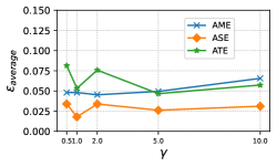
(a) $\alpha=0.5$

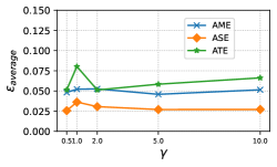
(b) $\alpha=1.0$

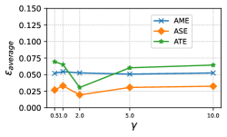
(c) $\alpha=2.0$

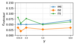
(d) $\alpha=0.5$

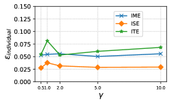
(e) $\alpha=1.0$

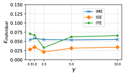
(f) $\alpha=2.0$

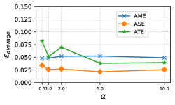
(g) $\gamma=0.5$

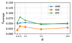
(h) $\gamma=1.0$

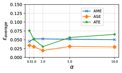
(i) $\gamma=2.0$

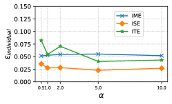
(j) $\gamma=0.5$

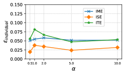
(k) $\gamma=1.0$

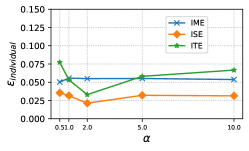
(l) $\gamma=2.0$

Figure 4: Additional hyperparameter sensitivity experimental results on BC.

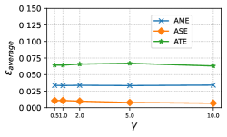
(a) $\alpha=0.5$

(b) $\alpha=1.0$

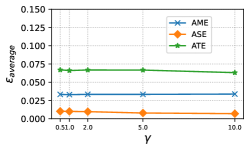
(c) $\alpha=2.0$

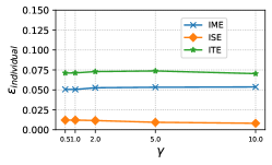
(d) $\alpha=0.5$

(e) $\alpha=1.0$

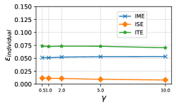
(f) $\alpha=2.0$

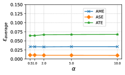
(g) $\gamma=0.5$

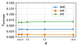
(h) $\gamma=1.0$

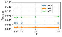
(i) $\gamma=2.0$

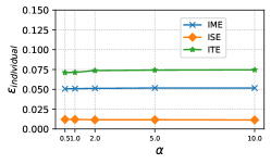
(j) $\gamma=0.5$

(k) $\gamma=1.0$

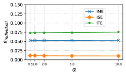
(l) $\gamma=2.0$

Figure 5: Additional hyperparameter sensitivity experimental results on BC(hete).

(a) $\alpha=0.5$

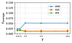
(b) $\alpha=1.0$

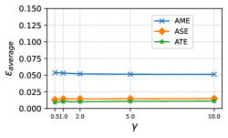
(c) $\alpha=2.0$

(d) $\alpha=0.5$

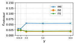
(e) $\alpha=1.0$

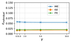
(f) $\alpha=2.0$

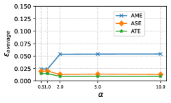
(g) $\gamma=0.5$

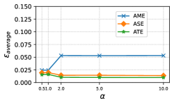
(h) $\gamma=1.0$

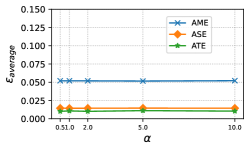
(i) $\gamma=2.0$

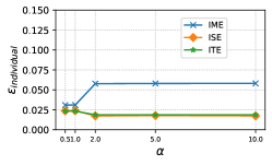
(j) $\gamma=0.5$

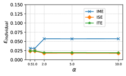
(k) $\gamma=1.0$

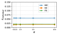
(l) $\gamma=2.0$

Figure 6: Additional hyperparameter sensitivity experimental results on Flickr.

(a) $\alpha=0.5$

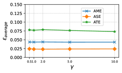
(b) $\alpha=1.0$

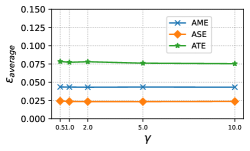
(c) $\alpha=2.0$

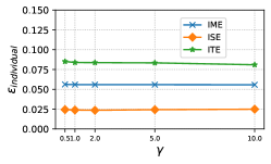
(d) $\alpha=0.5$

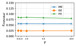
(e) $\alpha=1.0$

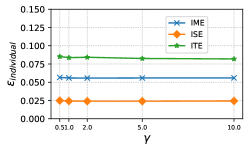
(f) $\alpha=2.0$

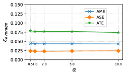
(g) $\gamma=0.5$

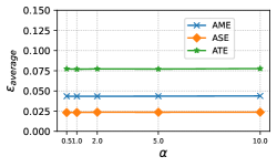
(h) $\gamma=1.0$

(i) $\gamma=2.0$

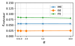
(j) $\gamma=0.5$

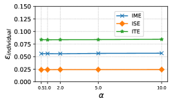
(k) $\gamma=1.0$

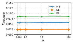
(l) $\gamma=2.0$

Figure 7: Additional hyperparameter sensitivity experimental results on Flickr(hete).

Table 5: Additional experimental MAPE results on the BC dataset. The top result is highlighted in bold, and the runner-up is underlined.

Metric	setting	effect	CFR+z	GEst	ND+z	NetEst	RRNet	NDR	Ours
$MAPE_{average}$	Within Sample	AME	$0.1009_{\pm 0.0678}$	$0.1901_{\pm 0.1076}$	$0.0868_{\pm 0.0794}$	$0.1192_{\pm 0.1284}$	$\underline{0.0795}_{\pm 0.0617}$	$0.5033_{\pm 0.0080}$	$0.0481_{\pm 0.0365}$
		ASE	$0.3910_{\pm 0.1164}$	$0.3366_{\pm 0.0269}$	$0.4275_{\pm 0.0601}$	$0.0576_{\pm 0.0318}$	$\underline{0.0462}_{\pm 0.0229}$	$0.4928_{\pm 0.0084}$	$0.0360_{\pm 0.0365}$
		ATE	$0.1401_{\pm 0.0907}$	$0.0738_{\pm 0.0519}$	$0.1870_{\pm 0.0536}$	$0.0579_{\pm 0.0308}$	$0.0413_{\pm 0.0400}$	$0.0142_{\pm 0.0074}$	$\underline{0.0267}_{\pm 0.0203}$
	Out-of Sample	AME	$0.1009_{\pm 0.0681}$	$0.1901_{\pm 0.1078}$	$0.0897_{\pm 0.0790}$	$0.1202_{\pm 0.1288}$	$\underline{0.0802}_{\pm 0.0623}$	/	$0.0481_{\pm 0.0364}$
		ASE	$0.3936_{\pm 0.1164}$	$0.3354_{\pm 0.0272}$	$0.4245_{\pm 0.0590}$	$0.0550_{\pm 0.0331}$	$\underline{0.0466}_{\pm 0.0237}$	/	$0.0357_{\pm 0.0366}$
		ATE	$0.1395_{\pm 0.0912}$	$0.0721_{\pm 0.0524}$	$0.1840_{\pm 0.0530}$	$0.0582_{\pm 0.0305}$	$\underline{0.0418}_{\pm 0.0400}$	/	$0.0266_{\pm 0.0203}$
$MAPE_{individual}$	Within Sample	IME	$0.1099_{\pm 0.0586}$	$0.2024_{\pm 0.0955}$	$0.0975_{\pm 0.0735}$	$0.1248_{\pm 0.1244}$	$\underline{0.0802}_{\pm 0.0611}$	/	$0.0486_{\pm 0.0360}$
		ISE	$0.3910_{\pm 0.1164}$	$0.3369_{\pm 0.0270}$	$0.4275_{\pm 0.0601}$	$0.0743_{\pm 0.0278}$	$\underline{0.0518}_{\pm 0.0199}$	/	$0.0372_{\pm 0.0361}$
		ITE	$0.1467_{\pm 0.0820}$	$0.0912_{\pm 0.0337}$	$0.1870_{\pm 0.0535}$	$0.0591_{\pm 0.0298}$	$\underline{0.0438}_{\pm 0.0378}$	/	$0.0273_{\pm 0.0196}$
	Out-of Sample	IME	$0.1113_{\pm 0.0575}$	$0.2014_{\pm 0.0968}$	$0.0999_{\pm 0.0739}$	$0.1262_{\pm 0.1245}$	$\underline{0.0808}_{\pm 0.0618}$	/	$0.0486_{\pm 0.0359}$
		ISE	$0.3936_{\pm 0.1164}$	$0.3358_{\pm 0.0273}$	$0.4245_{\pm 0.0590}$	$0.0716_{\pm 0.0263}$	$\underline{0.0523}_{\pm 0.0201}$	/	$0.0370_{\pm 0.0360}$
		ITE	$0.1477_{\pm 0.0803}$	$0.0894_{\pm 0.0345}$	$0.1843_{\pm 0.0527}$	$0.0594_{\pm 0.0296}$	$\underline{0.0443}_{\pm 0.0378}$	/	$0.0272_{\pm 0.0196}$

We add more experimental results, which are consistent with our analysis in the main body. Table 2 shows the performances of all baselines running on Flickr(homo) dataset. Table 3 shows the performances of all baselines running on the BC(hete) dataset. Table 4 shows the performances of all baselines running on the Flickr(hete) dataset. Figures 4, 5, 6, and 7 show the additional sensitivity results on the BC, BC(hete), Flickr, and Flickr(hete) datasets respectively.

It could be also informative to report MAPE as well. Thus, we provide alternative MAPE results for Table 1 in Table 5. Regarding AME, ASE and ATE, we use $MAPE_{average}=|\frac{\tau-\hat{\tau}}{\tau}|$. Regarding IME, ASE and ITE, we use $MAPE_{individual}=\sum_{i}^{n}||\frac{\tau_{i}-\hat{\tau_{i}}}{\tau_{i}}||$ where $n$ is the sample size.

Appendix J Additional Sensitivity Results on Hyperparameter $B$

We provide additional results by varying hyperparameter $B$ with fixed $\alpha=\beta=0.5$ on different datasets in Figure 8.

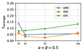
(a) on BC

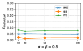
(b) on BC

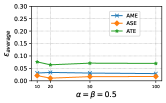
(c) on BC(hete)

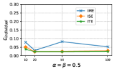
(d) on BC(hete)

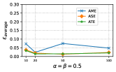
(e) on Flickr

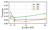
(f) on Flickr

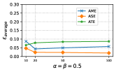
(g) on Flickr(hete)

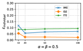
(h) on Flickr(hete)

Figure 8: Additional hyperparameter sensitivity experimental results on different datasets.

Appendix K Additional Results on Heterogenous Datasets

We also conduct experiments on simulated datasets to verify the effectiveness of the heterogeneous spillover effect estimation. Specifically, we reuse the datasets BC in our paper and modify their outcome model as follows:

$$y_{i}(t_{i},z_{i})=t_{i}+z_{i}+po_{i}+0.5\times po_{\mathcal{N}_{i}}+t_{i}\times(po_{i}+0.5\times po_{\mathcal{N}_{i}})+z_{i}\times(0.5\times po_{i}+po_{\mathcal{N}_{i}})+e_{i},$$ (35)

where $e_{i}$ is a Gaussian noise term. As same in our paper, $po_{i}=Sigmoid(w_{2}\times x_{i})$, and $po_{\mathcal{N}_{i}}$ is the averages of $po_{i}$. The term $z_{i}\times(0.5\times po_{i}+po_{\mathcal{N}_{i}})$ is introduced to allow heterogeneous spillover effects. We denote this dataset as BC(hete_z).

The experimental results on this dataset are shown in Figure 6. Compared with the existing methods, TNet performs better, showing lower bias in terms of estimation error. In particular, TNet performs the best in terms of average/individual spillover effect (ASE/AIE) estimation error, which means that TNet is capable of estimating heterogeneous spillover effects.

Table 6: Additional experimental results on the BC(hete_z) dataset. The top result is highlighted in bold, and the runner-up is underlined.

Metric	setting	effect	CFR+z	GEst	ND+z	NetEst	RRNet	NDR	Ours
$\varepsilon_{average}$	Within Sample	AME	$0.0824_{\pm 0.0786}$	$0.2254_{\pm 0.1597}$	$0.1383_{\pm 0.1019}$	$0.0770_{\pm 0.0425}$	$\underline{0.0653}_{\pm 0.0432}$	$0.8819_{\pm 0.0406}$	$\boldsymbol{0.0334_{\pm 0.0319}}$
		ASE	$0.2295_{\pm 0.0840}$	$0.0825_{\pm 0.0612}$	$0.2851_{\pm 0.0150}$	$0.0539_{\pm 0.0260}$	$\underline{0.0310}_{\pm 0.0241}$	$0.4366_{\pm 0.0182}$	$\boldsymbol{0.0183_{\pm 0.0125}}$
		ATE	$0.1925_{\pm 0.1465}$	$0.1375_{\pm 0.1017}$	$0.4325_{\pm 0.1982}$	$0.1782_{\pm 0.0800}$	$0.1342_{\pm 0.1177}$	$\boldsymbol{0.0836_{\pm 0.0357}}$	${\underline{0.0925}_{\pm 0.0443}}$
	Out-of Sample	AME	$0.0834_{\pm 0.0783}$	$0.2197_{\pm 0.1547}$	$0.1303_{\pm 0.0987}$	$0.0754_{\pm 0.0463}$	$\underline{0.0680}_{\pm 0.0464}$	/	$\boldsymbol{0.0341_{\pm 0.0310}}$
		ASE	$0.2279_{\pm 0.0837}$	$0.0808_{\pm 0.0624}$	$0.2831_{\pm 0.0118}$	$0.0517_{\pm 0.0274}$	$\underline{0.0327}_{\pm 0.0232}$	/	$\boldsymbol{0.0202_{\pm 0.0104}}$
		ATE	$0.1888_{\pm 0.1517}$	$0.1430_{\pm 0.1022}$	$0.4230_{\pm 0.2124}$	$0.1864_{\pm 0.0773}$	$\underline{0.1340}_{\pm 0.1225}$	/	$\boldsymbol{0.0953_{\pm 0.0433}}$
$\varepsilon_{individual}$	Within Sample	IME	$0.1314_{\pm 0.0645}$	$0.2638_{\pm 0.1370}$	$0.1971_{\pm 0.0754}$	$0.1284_{\pm 0.0227}$	$\underline{0.0864}_{\pm 0.0410}$	/	$\boldsymbol{0.0503_{\pm 0.0275}}$
		ISE	$0.2340_{\pm 0.0846}$	$0.1071_{\pm 0.0407}$	$0.2888_{\pm 0.0169}$	$0.0703_{\pm 0.0215}$	$\underline{0.0541}_{\pm 0.0184}$	/	$\boldsymbol{0.0359_{\pm 0.0057}}$
		ITE	$0.2460_{\pm 0.1184}$	$0.2077_{\pm 0.0707}$	$0.4803_{\pm 0.1674}$	$0.2362_{\pm 0.0644}$	$0.1542_{\pm 0.1075}$	/	$\boldsymbol{0.1065_{\pm 0.0396}}$
	Out-of Sample	IME	$0.1365_{\pm 0.0624}$	$0.2589_{\pm 0.1347}$	$0.2043_{\pm 0.0679}$	$0.1315_{\pm 0.0243}$	$\underline{0.0833}_{\pm 0.0452}$	/	$\boldsymbol{0.0513_{\pm 0.0266}}$
		ISE	$0.2327_{\pm 0.0844}$	$0.1074_{\pm 0.0405}$	$0.2877_{\pm 0.0141}$	$0.0693_{\pm 0.0188}$	$\underline{0.0537}_{\pm 0.0192}$	/	$\boldsymbol{0.0381_{\pm 0.0055}}$
		ITE	$0.2510_{\pm 0.1190}$	$0.2228_{\pm 0.0688}$	$0.4833_{\pm 0.1668}$	$0.2451_{\pm 0.0648}$	$\underline{0.1547}_{\pm 0.1130}$	/	$\boldsymbol{0.1109_{\pm 0.0387}}$

Appendix L Real-world Application

We apply our method to a real-world application, studying the impact of the installation of selective catalytic or selective non-catalytic reduction (SCR/SNCR) on the NO_x emissions of 473 power plants in America. This dataset is homologous to that used in (Papadogeorgou et al., 2019; Liu et al., 2023). Specifically, the installation of SCR/SNCR is the treatment variable, NO_x emission is selected as the outcome, and the 18 environmental factors are the covariates, including $4th$ maximum temperature over the study period and so on. Following (Liu et al., 2023), we select the five closest power plants as a power plant’s neighbors. The reason for selecting NO_x emissions as our outcome is that the analysis of NO_x is not expected to suffer from unmeasured spatial confounding as it is analyzed in (Papadogeorgou et al., 2019). Moreover, we estimate the confidence interval (CI) by the bootstrap method. Specifically, we run our methods serval times (e.g., 100 in the real-world experiment), and obtain the approximated confidence interval ($95\%$) using the resulting multiple estimated value by the bootstrap method. We use the SciPy library to get the CI.

Analysis: First, we found that the average main effect, $\hat{\psi}(1,0)-\hat{\psi}(0,0)$ is $-117.7$ ($95\%$ CI: $-127,-107$), indicating the installation of SCR/SNCR can reduce NO_x emissions. This result is consistent with [1] which shows that the installation of SCR/SNCR would reduce on average $205.1$ tons of NO_x emissions ($95\%$ CI $4,406$). Second, we found that $\hat{\psi}(1,z)-\hat{\psi}(1,0)$ with $z$ from $0.1$ to $0.4$ become smaller, i.e., $-117.2,160.4,117.2,47.1$ ($95\%$ CI $-121,-114$; $-165,-156$; $-123,-112$; $-53,-41$). One possible reason is that a plant power with SCR/SNCR installation would be a substitution for its neighbors without SCR/SNCR installation, making its larger NO_x emission reduction with less installation of SCR/SNCR of neighbor. Moreover, we observed that the total effect $\hat{\psi}(1,z)-\hat{\psi}(0,z)$ with $z$ from $0.1$ to $0.4$ become larger, i.e., $-151.5,-205.8,-319.0,-440.0$ ($95\%$ CI: $-169,-143$; $-213,-199$;$-326,-312$; $-447,-433$). This indicates that the more power plants install SCR/SNCR, the less NO_x they emit. Overall, our study underscores the effectiveness of SCR/SNCR installation in reducing NO_x emissions and indicates a potential substitution effect among neighboring plants. These findings contribute to a better understanding of the real-world implications of adopting emission reduction strategies in the energy industry.

References

• Assaad et al. (2021) Assaad, S., Zeng, S., Tao, C., Datta, S., Mehta, N., Henao, R., Li, F., and Carin, L. Counterfactual representation learning with balancing weights. In International Conference on Artificial Intelligence and Statistics, pp.  1972–1980. PMLR, 2021.
• Balzer et al. (2019) Balzer, L. B., Zheng, W., van der Laan, M. J., and Petersen, M. L. A new approach to hierarchical data analysis: Targeted maximum likelihood estimation for the causal effect of a cluster-level exposure. Statistical Methods in Medical Research, 28(6):1761–1780, 2019. doi: 10.1177/0962280218774936. URL https://doi.org/10.1177/0962280218774936. PMID: 29921160.
• Barkley et al. (2020) Barkley, B. G., Hudgens, M. G., Clemens, J. D., Ali, M., and Emch, M. E. Causal inference from observational studies with clustered interference, with application to a cholera vaccine study. Annals of Applied Statistics, 14(3):1432–1448, 2020.
• Bartlett & Mendelson (2002) Bartlett, P. L. and Mendelson, S. Rademacher and gaussian complexities: Risk bounds and structural results. Journal of Machine Learning Research, 3(Nov):463–482, 2002.
• Cai et al. (2023) Cai, R., Yang, Z., Chen, W., Yan, Y., and Hao, Z. Generalization bound for estimating causal effects from observational network data. In Proceedings of the 32nd ACM International Conference on Information and Knowledge Management, CIKM ’23, pp.  163–172, New York, NY, USA, 2023. Association for Computing Machinery. ISBN 9798400701245. doi: 10.1145/3583780.3614892. URL https://doi.org/10.1145/3583780.3614892.
• Cai et al. (2024) Cai, R., Chen, W., Yang, Z., Wan, S., Zheng, C., Yang, X., and Guo, J. Long-term causal effects estimation via latent surrogates representation learning. Neural Networks, 176:106336, 2024. ISSN 0893-6080. doi: https://doi.org/10.1016/j.neunet.2024.106336. URL https://www.sciencedirect.com/science/article/pii/S0893608024002600.
• Chen et al. (2023) Chen, D., Petersen, M. L., Rytgaard, H. C., Grøn, R., Lange, T., Rasmussen, S., Pratley, R. E., Marso, S. P., Kvist, K., Buse, J., and van der Laan, M. J. Beyond the cox hazard ratio: A targeted learning approach to survival analysis in a cardiovascular outcome trial application. Statistics in Biopharmaceutical Research, 15(3):524–539, 2023. doi: 10.1080/19466315.2023.2173644. URL https://doi.org/10.1080/19466315.2023.2173644.
• Chin (2019) Chin, A. Regression adjustments for estimating the global treatment effect in experiments with interference. Journal of Causal Inference, 7(2):20180026, 2019.
• Defferrard et al. (2016) Defferrard, M., Bresson, X., and Vandergheynst, P. Convolutional neural networks on graphs with fast localized spectral filtering. Advances in neural information processing systems, 29, 2016.
• Ferraro et al. (2019) Ferraro, P. J., Sanchirico, J. N., and Smith, M. D. Causal inference in coupled human and natural systems. Proceedings of the National Academy of Sciences, 116(12):5311–5318, 2019.
• Forastiere et al. (2021) Forastiere, L., Airoldi, E. M., and Mealli, F. Identification and estimation of treatment and interference effects in observational studies on networks. Journal of the American Statistical Association, 116(534):901–918, 2021.
• Guo et al. (2020) Guo, R., Li, J., and Liu, H. Learning individual causal effects from networked observational data. In Proceedings of the 13th International Conference on Web Search and Data Mining, pp.  232–240, 2020.
• Hines et al. (2022a) Hines, O., Dukes, O., Diaz-Ordaz, K., and Vansteelandt, S. Demystifying statistical learning based on efficient influence functions. The American Statistician, 76(3):292–304, 2022a. doi: 10.1080/00031305.2021.2021984. URL https://doi.org/10.1080/00031305.2021.2021984.
• Hines et al. (2022b) Hines, O., Dukes, O., Diaz-Ordaz, K., and Vansteelandt, S. Demystifying statistical learning based on efficient influence functions. The American Statistician, 76(3):292–304, 2022b.
• Huang (2003) Huang, J. Z. Local asymptotics for polynomial spline regression. The Annals of Statistics, 31(5):1600 – 1635, 2003. doi: 10.1214/aos/1065705120. URL https://doi.org/10.1214/aos/1065705120.
• Huang et al. (2002) Huang, J. Z., Wu, C. O., and Zhou, L. Varying-coefficient models and basis function approximations for the analysis of repeated measurements. Biometrika, 89(1):111–128, 2002.
• Huang et al. (2004) Huang, J. Z., Wu, C. O., and Zhou, L. Polynomial spline estimation and inference for varying coefficient models with longitudinal data. Statistica Sinica, pp.  763–788, 2004.
• Jiang & Sun (2022) Jiang, S. and Sun, Y. Estimating causal effects on networked observational data via representation learning. In Proceedings of the 31st ACM International Conference on Information & Knowledge Management, pp.  852–861, 2022.
• Johansson et al. (2016) Johansson, F., Shalit, U., and Sontag, D. Learning representations for counterfactual inference. In International conference on machine learning, pp. 3020–3029. PMLR, 2016.
• Johansson et al. (2021) Johansson, F. D., Shalit, U., Kallus, N., and Sontag, D. Generalization bounds and representation learning for estimation of potential outcomes and causal effects, 2021.
• Kennedy et al. (2017) Kennedy, E. H., Ma, Z., McHugh, M. D., and Small, D. S. Non-parametric methods for doubly robust estimation of continuous treatment effects. Journal of the Royal Statistical Society Series B: Statistical Methodology, 79(4):1229–1245, 2017.
• Kingma & Ba (2014) Kingma, D. P. and Ba, J. Adam: A method for stochastic optimization. arXiv preprint arXiv:1412.6980, 2014.
• Kipf & Welling (2016) Kipf, T. N. and Welling, M. Semi-supervised classification with graph convolutional networks. In International Conference on Learning Representations, 2016.
• Kreif et al. (2017) Kreif, N., Tran, L., Grieve, R., De Stavola, B., Tasker, R. C., and Petersen, M. Estimating the Comparative Effectiveness of Feeding Interventions in the Pediatric Intensive Care Unit: A Demonstration of Longitudinal Targeted Maximum Likelihood Estimation. American Journal of Epidemiology, 186(12):1370–1379, 06 2017. ISSN 0002-9262. doi: 10.1093/aje/kwx213. URL https://doi.org/10.1093/aje/kwx213.
• Künzel et al. (2019) Künzel, S. R., Sekhon, J. S., Bickel, P. J., and Yu, B. Metalearners for estimating heterogeneous treatment effects using machine learning. Proceedings of the national academy of sciences, 116(10):4156–4165, 2019.
• Lee et al. (2021) Lee, T., Buchanan, A. L., Katenka, N. V., Forastiere, L., Halloran, M. E., Friedman, S. R., and Nikolopoulos, G. Estimating causal effects of hiv prevention interventions with interference in network-based studies among people who inject drugs. arXiv preprint arXiv:2108.04865, 2021.
• Li et al. (2018) Li, F., Morgan, K. L., and Zaslavsky, A. M. Balancing covariates via propensity score weighting. Journal of the American Statistical Association, 113(521):390–400, 2018.
• Liu et al. (2023) Liu, J., Ye, F., and Yang, Y. Nonparametric doubly robust estimation of causal effect on networks in observational studies. Stat, 12(1):e549, 2023.
• Liu et al. (2016) Liu, L., Hudgens, M. G., and Becker-Dreps, S. On inverse probability-weighted estimators in the presence of interference. Biometrika, 103(4):829–842, 2016.
• Ma et al. (2021) Ma, J., Guo, R., Chen, C., Zhang, A., and Li, J. Deconfounding with networked observational data in a dynamic environment. In Proceedings of the 14th ACM International Conference on Web Search and Data Mining, pp.  166–174, 2021.
• Ma et al. (2022) Ma, J., Wan, M., Yang, L., Li, J., Hecht, B., and Teevan, J. Learning causal effects on hypergraphs. In Proceedings of the 28th ACM SIGKDD Conference on Knowledge Discovery and Data Mining, pp.  1202–1212, 2022.
• Ma & Tresp (2021) Ma, Y. and Tresp, V. Causal inference under networked interference and intervention policy enhancement. In International Conference on Artificial Intelligence and Statistics, pp.  3700–3708. PMLR, 2021.
• McNealis et al. (2023) McNealis, V., Moodie, E. E., and Dean, N. Doubly robust estimation of causal effects in network-based observational studies. arXiv preprint arXiv:2302.00230, 2023.
• Nie et al. (2020) Nie, L., Ye, M., Nicolae, D., et al. Vcnet and functional targeted regularization for learning causal effects of continuous treatments. In International Conference on Learning Representations, 2020.
• Nie et al. (2021) Nie, L., Ye, M., qiang liu, and Nicolae, D. Varying coefficient neural network with functional targeted regularization for estimating continuous treatment effects. In International Conference on Learning Representations, 2021. URL https://openreview.net/forum?id=RmB-88r9dL.
• Papadogeorgou et al. (2019) Papadogeorgou, G., Choirat, C., and Zigler, C. M. Adjusting for unmeasured spatial confounding with distance adjusted propensity score matching. Biostatistics, 20(2):256–272, 2019.
• Parshakov et al. (2020) Parshakov, P., Naidenova, I., and Barajas, A. Spillover effect in promotion: Evidence from video game publishers and esports tournaments. Journal of Business Research, 118:262–270, 2020.
• Pearl (2009) Pearl, J. Causality. Cambridge university press, 2009.
• Robins et al. (1994) Robins, J. M., Rotnitzky, A., and Zhao, L. P. Estimation of regression coefficients when some regressors are not always observed. Journal of the American statistical Association, 89(427):846–866, 1994.
• Rosenbaum (1987) Rosenbaum, P. R. Model-based direct adjustment. Journal of the American Statistical Association, 82(398):387–394, 1987.
• Rosenbaum & Rubin (1983) Rosenbaum, P. R. and Rubin, D. B. The central role of the propensity score in observational studies for causal effects. Biometrika, 70(1):41–55, 1983.
• Rosenbaum & Rubin (1985) Rosenbaum, P. R. and Rubin, D. B. Constructing a control group using multivariate matched sampling methods that incorporate the propensity score. The American Statistician, 39(1):33–38, 1985.
• Rubin (1974) Rubin, D. B. Estimating causal effects of treatments in randomized and nonrandomized studies. Journal of educational Psychology, 66(5):688, 1974.
• Schumaker (2007) Schumaker, L. Spline functions: basic theory. Cambridge university press, 2007.
• Shi et al. (2019) Shi, C., Blei, D., and Veitch, V. Adapting neural networks for the estimation of treatment effects. Advances in neural information processing systems, 32, 2019.
• van der Laan & Gruber (2012) van der Laan, M. J. and Gruber, S. Targeted minimum loss based estimation of causal effects of multiple time point interventions. The International Journal of Biostatistics, 8(1), 2012. doi: doi:10.1515/1557-4679.1370. URL https://doi.org/10.1515/1557-4679.1370.
• van der Laan & Rubin (2006) van der Laan, M. J. and Rubin, D. Targeted maximum likelihood learning. The International Journal of Biostatistics, 2(1), 2006. doi: doi:10.2202/1557-4679.1043. URL https://doi.org/10.2202/1557-4679.1043.
• Van der Laan et al. (2011) Van der Laan, M. J., Rose, S., et al. Targeted learning: causal inference for observational and experimental data, volume 4. Springer, 2011.
• Veitch et al. (2019) Veitch, V., Wang, Y., and Blei, D. Using embeddings to correct for unobserved confounding in networks. Advances in Neural Information Processing Systems, 32, 2019.
• Wang et al. (2008) Wang, L., Li, H., and Huang, J. Z. Variable selection in nonparametric varying-coefficient models for analysis of repeated measurements. Journal of the American Statistical Association, 103(484):1556–1569, 2008.