Quantum Algorithms for Inverse Participation Ratio Estimation in multi-qubit and multi-qudit systems

Abstract

Inverse Participation Ratios (IPRs) and the related Participation Entropies quantify the spread of a quantum state over a selected basis of the Hilbert space, offering insights into the equilibrium and non-equilibrium properties of the system. In this work, we propose three quantum algorithms to estimate IPRs on multi-qubit and multi-qudit quantum devices. The first algorithm allows for the estimation of IPRs in the computational basis by single-qubit measurements, while the second one enables measurement of IPR in the eigenbasis of a selected Hamiltonian, without the knowledge about the eigenstates of the system. Next, we provide an algorithm for IPR in the computational basis for a multi-qudit system. We discuss resources required by the algorithms and benchmark them by investigating the one-axis twisting protocol, the thermalization in a deformed PXP model, and the ground state of a spin-$1$ AKLT chain in a transverse field.

1 Introduction

Understanding equilibrium [1, 2, 3, 4] and non-equilibrium [5, 6, 7, 8, 9, 10] properties of quantum many-body systems is a significant challenge in contemporary physics [11]. While investigations of many-body systems on classical computers are hindered by the exponential growth of the Hilbert space dimension with the system size, the recent experimental breakthroughs in realizing and controlling synthetic matter platforms fulfill the vision of quantum simulation [12, 13, 14, 15] proposed by R. Feynman [16]. Moreover, quantum computing has already reached a point in which non-trivial computational tasks may be performed in gate-based settings on quantum processors [17, 18, 19] despite operating in the presence of noise and errors and still belonging to the Noisy Intermediate-Scale Quantum (NISQ) era [20].

The research of quantum algorithms, whose paradigmatic examples include algorithms for integer factorization [21], unstructured database search [22] or quantum phase estimation algorithm  [23], has been intensified due to the advancements of quantum processors during the NISQ era, as reviewed in [24, 25]. Examples include quantum algorithmic solutions for quantum dynamics [26, 27] allowing for simulation of time evolution of many-body systems [28, 29], finding the energy spectrum of a static Hamiltonian [30, 31], or approximating thermal states [32, 33, 34]. These explorations not only open the door for discoveries in large-scale quantum many-body systems [35, 36, 37, 38, 39] but also provide ways of benchmarking the quantum hardware [40]. Variational quantum algorithms that leverage classical optimization techniques to train parameterized quantum circuits [41, 42, 43, 44] constitute another group of methods aimed at addressing the constraints of a limited number of qubits and noise characteristic for quantum processors from the NISQ era.

Among various types of quantum algorithms, approaches aimed at quantifying the properties of the quantum state are of pivotal importance for building, calibrating, and controlling quantum systems. Quantum state tomography, i.e., a complete reconstruction of a quantum state [45, 46] has limited applications in many-body systems due to the exponential growth of the Hilbert space dimension with qubit number. This lead to the development of approaches such as shadow tomography [47] or randomized measurement toolbox [48] aimed at quantifying specific properties of quantum states including higher order correlation functions [49], entanglement entropies [50, 51, 52, 53], out-of-time-order correlations [54, 55] or stabilizer Renyi entropies [56] which quantify the non-Clifford resources required to prepare the state [57].

In this work, we focus on the inverse participation ratios (IPRs) and the related participation entropies, which quantify the spread of state $|\psi\rangle$ in a selected basis $\mathcal{B}$ of the Hilbert space of quantum many-body system. We propose quantum algorithms to estimate IPRs in the computational basis and in the eigenbasis of a selected Hamiltonian. The introduced algorithms are benchmarked with exact numerical computations. This paper is organized as follows. In Sec. 2, we introduce the notions of IPRs and participation entropies, commenting on their relevance for quantum many-body systems. Next, in Sec. 3, we propose quantum algorithms to estimate IPR in the computational basis and in the eigenbasis of a Hamiltonian for qubits and qudits. Relevant examples, numerical results, and simulations on quantum processors are presented in Sec. 4. In Sec. 5, we conclude and discuss the utility of the introduced algorithms for near-term quantum computing.

2 Inverse Participation Ratios

Let us consider the arbitrary many-body hermitian operator $\hat{A}$ and the complete many-body basis ${\cal B}_{A}=\{|i\rangle\}$ in which operator $\hat{A}$ is diagonal. Any pure quantum state $|\psi\rangle$ can be decomposed as $|\psi\rangle=\sum_{i}c_{i}|i\rangle$, where $c_{i}=\langle i|\psi\rangle$. To quantify properties of $|\psi\rangle$, we consider the IPRs defined as

$$I^{A}_{q}=\sum_{i=0}^{{\cal N}-1}|c_{i}|^{2q},\quad q=2,3,4\cdots,$$ (1)

where ${\cal N}=d^{L}$ is the dimension of the Hilbert space, $d$ is local Hilbert space size, and the integer $q\geq 2$ is referred to as the Rényi index. The IPR $I^{A}_{q}$ takes values in the range $[{\cal N}^{1-q},1]$. The lower bound corresponds to the case when $|\psi\rangle$ uniformly populates all the basis states, namely, $|c_{i}|^{2}={\cal N}^{-1}$. The upper bound is admitted when $|\psi\rangle$ is fully localized on a single basis state $|j\rangle$, i.e., $c_{i}=\delta_{i,j}$. The IPRs have been one of the main tools in assessing the localization properties of single particle wave functions across the Anderson localization transition [58, 59, 60, 61, 62], including recent investigations of the Anderson model on hierarchical graphs [63, 64, 65, 66, 67, 68, 69, 70].

For a system of $L$ qubits, $d=2$, the Hilbert space dimension is ${\cal N}=2^{L}$, which implies that $I^{A}_{q}$ may be exponentially small in the system size $L$, motivating introduction of the participation entropies $S_{q}$, defined as Rényi entropies of the probability distribution $p_{i}=|c_{i}|^{2}$,

$$S_{q}=\dfrac{1}{1-q}\log_{2}I^{A}_{q},\quad q=2,3,4\cdots.$$ (2)

which constitute a related measure of the spread of $|\psi\rangle$ in the basis ${\cal B}_{A}$. The system size dependence of the participation entropy can be parameterized, in a sufficiently narrow interval of system sizes, as $S_{q}=D_{q}\log_{2}{\cal N}+c_{q}$ where $D_{q}$ is a fractal dimension [71], $c_{q}$ is a sub-leading term. If the analyzed state $\ket{\psi}$ is localized on a fixed number of basis states, the participation entropy $S_{q}$ is independent of $L$, resulting in a vanishing fractal dimension $D_{q}=0$. In contrast, a multi-qubit state uniformly delocalized over the basis ${\cal B}_{A}$, $|c_{i}|^{2}={\cal N}^{-1}$, is characterized by $D_{q}=1$. Similarly, Haar-random states, obtained as $\ket{\psi}=U\ket{\psi_{0}}$, where $\ket{\psi_{0}}$ is a fixed state and $U$ is a matrix drawn with Haar measure from the unitary group on $L$ qubits, are fully delocalized in the Hilbert space, with the fractal dimension $D_{q}=1$ (and a sub-leading term $c_{q}<0$) [72]. Multifractality [73, 74] is the intermediate case between the delocalization ($D_{q}=1$) and localization ($D_{q}=0$) when the fractal dimension $0<D_{q}<1$ depends non-trivially on the Rényi index $q$.

The participation entropies of ground states of quantum many-body systems have been employed to distinguish between various quantum phases [75, 76, 77, 78, 79, 80, 81, 82, 83]. Moreover, participation entropies can be used as an ergodicity breaking measure in quantum many-body systems as proposed in [84]. Indeed, while the properties eigenstates of thermalizing [85, 86, 87, 88, 89] many-body systems may be modeled by the fully delocalized random Haar states, ergodicity breaking due to many-body localization [90, 91, 8, 10] is manifested by the multifractality of many-body states [92]. Similarly, measurement-induced phase transitions in unitary dynamics of random circuits [9] interspersed with local measurements can be investigated through the lens of participation entropies [93, 94]. The IPRs and participation entropies can be also used to probe time dynamics of quantum circuits [95] and are related to the relative entropies of coherence [96] important for the resource theory of quantum coherence [97], and stabilizer Renyi entropies [98]. Finally, the IPR $I_{2}$ coincides with a collision probability describing the anticoncentration properties of the many-body wave function, relevant for the formal arguments of classical hardness of the sampling problems [99, 100, 101, 102].

The broad relevance of the IPRs and participation entropies to quantum many-body systems motivates us to consider quantum algorithms for their measurement. For concreteness, since IPRs and participation entropies are functionally dependent, c.f. (2), we focus on measuring the IPRs (1).

3 Quantum algorithms for IPR estimation

In this section, we introduce the primary algorithm developed within this paper. Subsection 3.1 details the algorithm for computing the Inverse Participation Ratio in the computational basis. Subsequently, in Subsection 3.2, we extend this algorithm to calculate the IPR in the eigenbasis of a chosen Hamiltonian for qubits. Finally, in Subsection 3.3, we generalize the computation of the IPR in the computational basis for qudits.

3.1 IPR in the computational basis for qubits

We consider a multi-qubit state $\ket{\psi}$ and fix the basis of interest as the computational basis, i.e. the eigenbasis of Pauli-Z operators, $\mathcal{B}_{Z}=\{\ket{\sigma_{i}}\}$, where $\sigma_{i}=0,1$. A naive experimental procedure for measuring IPRs in the computational basis could consist of performing the measurements of the $\hat{Z}$ operators, recording the resulting bitstrings associated with the basis states $\ket{\sigma_{i}}$, estimating the probabilities $|c_{i}|^{2}=|\langle\sigma_{i}\ket{\psi}|^{2}$ and calculating the IPRs using their definition Eq.(1). While the procedure of such a sampling of the state is experimentally realized on quantum processors [17] and forms a basis of the cross-entropy benchmarking [103], it requires estimation of exponentially many probabilities $|c_{i}|^{2}$ associated with each of the states of $\mathcal{B}_{Z}$.

[row sep=0.4cm, column sep=0.4cm] 0& H 1 H
ψ [2, disable auto height] Π_qwide
$\ket{\psi}^{\otimes q-1}$ 1
$\ket{0}^{\otimes n\times(q-1)}$

Figure 1: Quantum circuit for estimating IPR $I^{Z}_{q}$ of Rényi index $q\geq 2$ in the computational basis $\mathcal{B}_{Z}$. The quantum circuit comprises $n\times(q-1)$ CNOT gates and a controlled-$\Pi_{q}$ gate. The value of $I^{Z}_{q}$ is determined as an expectation value of the Pauli-Z operator on the ancillary qubit.

In the following, we propose a quantum algorithm that allows the measurement of IPR in a computational basis, denoted as $I^{Z}_{q}$, as an expectation value of a single-qubit measurement.

The algorithm requires $q$ copies of the state $|\psi\rangle=\sum_{i}c_{i}\ket{i}$ (where the index $i$ runs over the states of the computational basis $\mathcal{B}_{Z}$) and additional $n$-qubit quantum registers, so that the input state reads

$$|\Psi_{0}\rangle= |0\rangle\otimes|\psi\rangle\otimes|\psi\rangle^{\otimes q-1}\otimes|0\rangle^{\otimes n(q-1)},$$

$$= \sum_{i_{0},\cdots,i_{q-1}}c_{i_{1}}\cdots c_{i_{q-1}}|0\rangle\otimes|i_{0},\cdots,i_{q-1}\rangle\otimes|0\rangle^{\otimes n(q-1)}.$$ (3)

The algorithm generates entanglement between the $(q-1)$ copies of $|\psi\rangle$ and the $n$-qubit quantum registers using the CNOT gates

$$U^{\otimes n(q-1)}_{\text{CNOT}}|\Psi_{0}\rangle= \sum_{i_{0},\cdots,i_{q-1}}c_{i_{0}}\cdots c_{i_{q-1}}|0\rangle\otimes|i_{0}\rangle$$

$$\otimes|i_{1},\cdots,i_{q-1}\rangle\otimes|i_{1},\cdots,i_{q-1}\rangle.$$ (4)

Subsequently, one ancillary qubit controls a cyclic permutation, denoted as a controlled-$\Pi_{q}$ gate in Figure 1. $\Pi_{q}$ acts on the $q$ systems as

$$\Pi_{q}|v_{0}\rangle\otimes|v_{1}\rangle\cdots\otimes|v_{q-1}\rangle=|v_{q-1}\rangle\otimes|v_{0}\rangle\cdots\otimes|v_{q-2}\rangle.$$ (5)

Two Hadamard gates $H$ and the controlled-$\Pi_{q}$ create a superposition of the permuted and non-permuted states, leading to the following output state

$$\ket{\Psi_{f}}=\frac{1}{\sqrt{2}}\left(\ket{+}\otimes\ket{\phi_{I}}+\ket{-}\otimes\ket{\phi_{C}}\right),$$ (6)

where $\ket{\pm}=\frac{1}{\sqrt{2}}(\ket{1}\pm\ket{0})$,

$$\ket{\phi_{I}}=\sum c_{i_{0}}\cdots c_{i_{q-1}}|i_{0},i_{1},\cdots,i_{q-1}\rangle\otimes|i_{1},\cdots,i_{q-1}\rangle,$$

$$\ket{\phi_{C}}=\sum c_{i_{0}}\cdots c_{i_{q-1}}|i_{q-1},i_{0},\cdots,i_{q-2}\rangle\otimes|i_{1},\cdots,i_{q-1}\rangle,$$

and the sums in $\ket{\phi_{I,C}}$ extend over all the indices $i_{0},\cdots,i_{q-1}$. Observing that $\langle\phi_{C}|\phi_{C}\rangle=1=\langle\phi_{I}|\phi_{I}\rangle$ due to the normalization of $\ket{\psi}$, while $\langle\phi_{C}|\phi_{I}\rangle=\sum_{i}|c_{i}|^{2q}$, we find the probability $P_{0}$ to find the ancilla qubit in state $|0\rangle$, given as $\langle\Psi_{f}|\left(|0\rangle\langle 0|\otimes\mathbb{1}\right)|\Psi_{f}\rangle$ reads

$$P_{0}=\dfrac{1}{2}+\dfrac{\sum_{i}|c_{i}|^{2q}}{2}=\frac{1}{2}+\frac{1}{2}I^{{}_{Z}}_{q}.$$ (7)

Hence, the IPR $I^{Z}_{q}$ can be directly obtained from the single-qubit measurements. Repeating the measurement of the Pauli-Z operator on the ancillary qubit $N_{\text{s}}$ times, the average of the results approaches the value of $P_{1}$ up to a statistical uncertainty scaling as $\epsilon\sim N_{\text{s}}^{-1/2}$. To enhance accuracy and reduce statistical errors, one available approach is the implementation of quantum amplitude estimation [104]. Our quantum algorithm can also be extended to an arbitrary basis $\{|b_{i}\rangle\}$. In that case, an additional unitary transform $V=\sum_{j}e^{-\text{i}\phi_{j}}|j\left\rangle\right\langle b_{j}|$ between computational basis and $\{|b_{i}\rangle\}$ is implemented before the $U_{\text{CNOT}}$ gates in Eq.(3.1).

We note that for the specific choice of $q=2$, the controlled-$\Pi_{2}$ is equivalent to a controlled-SWAP gate. Then, the ancillary qubit implements the SWAP test protocol [105], returning fidelity between $|\psi\rangle$ and reduced quantum state $\rho=\sum_{i}|c_{i}|^{2}|i\rangle\langle i|$.

Finally, we comment on the resources required by our algorithm. In comparison to the requirement of $L$ measurements required to estimate the probabilities $|c_{i}|^{2}=|\langle i\ket{\psi}|^{2}$ in the computational basis $\mathcal{B}_{Z}$, our algorithm requires only a single qubit measurement.

However, in general, the IPRs may be exponentially small in system size $L$. In such cases, exponentially small statistical error $\epsilon$, and consequently, an exponentially large $N_{s}$, may be required to achieve an accurate estimation of the IPRs. To illustrate this, we consider the following examples

• a basis state $\ket{\sigma_{i}}$ in the computational basis, for which $I^{Z}_{q}=1$. In that case, statistical error $\sigma\approx O(1)$ is sufficient to reach a small relative error of $I^{Z}_{q}$;

• a GHZ state $\ket{\mathrm{GHZ}}=\frac{1}{\sqrt{2}}\left(|1\rangle^{\otimes L}+|0\rangle^{\otimes L}\right)$, for which $I^{Z}_{q}=2^{1-q}$. In spite of the non-trivial entanglement structure of this state, a statistical error of $\sigma\approx O(1)$ is sufficient for any $q\geq 2$;

• a product state

  $$\ket{\theta}=\left(\cos(\theta)\ket{0}+\sin(\theta)\ket{1})\right)^{\otimes L};$$ (8)

  for which $I^{Z}_{q}=\left(\cos^{2q}(\theta)+\sin^{2q}(\theta)\right)^{L}$. For a generic value of $\theta$, the IPR is exponentially small in the system size $L$. To resolve such a quantity, an exponentially large $N_{s}$ is required;

• random Haar state, for which $I^{Z}_{q}\propto 2^{(1-q)L}$. In that case, $N_{s}$ scaling exponentially with $L$ is required for an accurate estimation of the IPRs.

These considerations show the practical difficulties encountered when estimating the IPRs, associated with the possible exponential smallness of the estimated quantity. This property reflects the fact the IPRs, by their construction, quantify the properties of many-body wave functions in the full many-body Hilbert space. As shown by the example of the product state, local rotations of the basis (e.g. fixing $\theta=0$) may dramatically decrease the resources needed for the estimation of IPRs. For certain tasks associated with assessing the dynamical properties of many-body systems, the eigenbasis of the Hamiltonian is distinguished, motivating the considerations of the following section.

[row sep=0.10cm, column sep=0.10cm] 0 & H1 52 [4, nwires=3]QFT3 [4]
   ⋮ 
0 H 3
0 H 2
ψ U^2^0 U^2^1 …U^2^m-1
ψ U^†^2^0 U^†^2^1 … U^†^2^m-1

Figure 2: Quantum circuit for estimating the IPR $I^{\cal H}_{2}$ in the eigenbasis $\mathcal{B}_{\mathcal{H}}$ of Hamiltonian $\hat{\mathcal{H}}$. The quantum circuit operates on two copies of the considered state $\ket{\psi}$ and $m$ ancillary qubits, and involves the action of the evolution operator $U$ and QFT. Measurement of the ancillary qubits allows us to estimate the value of $I^{\cal H}_{2}$.

3.2 IPR in eigenbasis of a selected Hamiltonian for qubits

In this section, we introduce a quantum algorithm for the calculation of IPR, denoted as $I^{\cal H}_{2}$ in an eigenbasis $\mathcal{B}_{\mathcal{H}}$ of a selected Hamiltonian $\hat{\mathcal{H}}$. When a many-body system is initially prepared in a state $\ket{\psi_{0}}$, a survival probability defined as $|\langle\psi_{0}\ket{\psi(t)}|^{2}$, where $\ket{\psi(t)}=e^{-\text{i}\hat{\mathcal{H}}t}\ket{\psi_{0}}$, provides means of assessing ergodicity and ergodicity breaking in the system [106, 107, 108, 109, 110, 111, 112, 113, 114]. Using the eigendecomposition of the Hamiltonian, $\hat{\mathcal{H}}\ket{\varepsilon_{i}}=\varepsilon_{i}\ket{\varepsilon_{i}}$, and assuming the lack of degeneracy of the eigenvalues $\varepsilon_{i}$, we find that the long-time average of the survival probability,

$$\lim_{\tau\rightarrow\infty}\frac{1}{\tau}\int_{0}^{\tau}dt|\langle\psi(t)|\psi_{0}\rangle|^{2}=\sum_{i}|\langle\varepsilon_{i}\ket{\psi_{0}}|^{4}=I^{{\cal H}}_{2},$$ (9)

is equal to the IPR with Rényi index $q=2$ of the initial state $\ket{\psi_{0}}$ in the eigenbasis $\mathcal{B}_{\mathcal{H}}=\{\ket{\varepsilon_{i}}\}$ of the Hamiltonian $\hat{\mathcal{H}}$. This motivates us to introduce the following quantum algorithm to calculate $I^{\cal H}_{2}$ in the basis $\mathcal{B}_{\mathcal{H}}$.

Without prior knowledge of the eigenbasis $\mathcal{B}_{\mathcal{H}}$ of $\hat{\mathcal{H}}$, estimation of $I^{{\cal H}}_{2}$ may be implemented via the quantum algorithm shown in Figure 2. The initial state is prepared as $|\Psi_{0}\rangle=|0\rangle^{\otimes m}|\psi\rangle^{\otimes 2}$, where $m$ denotes the number of ancillary qubits. The algorithm commences by application of Hadamard gates onto the $m$ ancillary qubits, followed by the controlled-$U$ and controlled-$U^{\dagger}$ operations on the two copies of the states $|\psi\rangle$ with the evolution operator $U=e^{-\text{i}\hat{\mathcal{H}}t}$ raised to successive powers of two. In result, the evolution of $|\psi\rangle^{\otimes 2}$ is controlled by the ancillary qubits $|x\rangle$ and involves operators $U^{x}\otimes{U^{\dagger}}^{x}$, where $x\in\{0,\cdots,2^{m}-1\}$ denotes the number of the $m$-th bit string. Subsequently, the quantum Fourier transform (QFT) [115, 116] module implements discrete Fourier transform over the ancillary qubits,

$$|x\rangle\xrightarrow{\text{QFT}}\frac{1}{\sqrt{2^{m}}}\sum_{k=0}^{2^{m}-1}e^{\text{i}\frac{2\pi xk}{2^{m}}}|k\rangle.$$ (10)

At the end of the circuit, measurements on the product of Pauli-Z strings $\hat{Z}^{\otimes m}$ are implemented.

More concretely, the input state undergoes the following evolution (see Figure 2)

$$|\Psi_{0}\rangle\xrightarrow{1} \dfrac{1}{\sqrt{2^{m}}}\sum_{x=0}^{2^{m}-1}|x\rangle\otimes|\varphi\rangle\otimes|\varphi\rangle,$$

$$\xrightarrow{2} \dfrac{1}{\sqrt{2^{m}}}\sum_{x=0}^{2^{m}-1}|x\rangle\otimes U^{x}\sum_{i}c_{i}|\varepsilon_{i}\rangle\otimes U^{-x}\sum_{j}c_{j}|\varepsilon_{j}\rangle,$$

$$= \sum_{i,j}\dfrac{c_{i}c_{j}}{\sqrt{2^{m}}}\sum_{x=0}^{2^{m}-1}|x\rangle\otimes e^{-\text{i}\tilde{\varepsilon}_{ij}tx}|\varepsilon_{i}\rangle|\varepsilon_{j}\rangle,$$

$$\xrightarrow{3} \sum_{i,j}\dfrac{c_{i}c_{j}}{2^{m}}\sum_{x=0}^{2^{m}-1}\left(\sum_{k=0}^{2^{m}-1}e^{\text{i}\frac{2\pi xk}{2^{m}}}|k\rangle\right)\otimes e^{-\text{i}\tilde{\varepsilon}_{ij}xt}|\varepsilon_{i}\rangle|\varepsilon_{j}\rangle,$$ (11)

where the energy difference $(\varepsilon_{i}-\varepsilon_{j})$ is abbreviated as $\tilde{\varepsilon}_{ij}$. The probability to measure $\{0\}^{m}$ on the ancillary qubits on the output state $\Psi_{\text{out}}$ is given by

$$P_{{0,m}} =\left<\Psi_{\text{out}}\right|(\left|0\right\rangle\left\langle 0\right|^{\otimes m}\otimes\mathbb{1})\left|\Psi_{\text{out}}\right\rangle=I^{\cal H}_{2}+\epsilon_{r},$$ (12)

where $I^{{\cal H}}_{2}$ is the IPR of $\ket{\psi}$ in the eigenbasis $\mathcal{B}_{\mathcal{H}}$ and $0\leq\epsilon_{r}\leq 4^{-m}\frac{\pi^{2}}{2\Delta^{2}t^{2}}$ with $\Delta$ denoting the minimum gap in the energy spectrum of $\hat{\mathcal{H}}$.

Notably, the upper bound of the error decreases exponentially with the number $m$ of ancillary qubits, which is a result of deploying an exponentially large in $m$ power of the operator $U$. The detailed proof of Eq. (12) and error analysis of $\epsilon_{r}$ are provided in Appendix A.

The realization of the controlled-$U$ operation is a crucial step in the proposed quantum algorithm as it allows for encoding of the information about the eigenstates and the corresponding phase factors into the phases of ancilla qubit states.

The evolution operator $U$ may be implemented via Suzuki-Trotter decomposition [117, 118]. The involved approximation results in a discrepancy between the exact time-evolution operator $e^{-\text{i}\hat{\mathcal{H}}t}$ and its approximation $U_{t}$, which can be quantified via $\epsilon_{t}=\parallel U_{t}-e^{-\text{i}{\cal H}t}\parallel$. It can be shown that $\epsilon_{t}\leq\frac{\parallel{\cal H}\parallel^{2}t^{2}}{2n_{T}}$ for the first-order Trotterization, with $n_{T}$ referring to the trotter steps [119]. Assuming that the number of gates in first-order Trotterization is $N_{t}$, the total number of gates for the algorithm in Figure 2 is $\mathcal{O}(2^{m+1}N_{t}+m^{2})$.

3.3 IPR in computational basis for qudits

[row sep=0.4cm, column sep=0.4cm] 0& H 1 H
ψ [2, disable auto height]Π_qwide
$\ket{\psi}^{\otimes q-1}$ [2, disable auto height]SUM
$\ket{0}^{\otimes n\times(q-1)}$

Figure 3: Generalized quantum circuit for estimating IPR $I^{Z}_{q}$ in the computational basis $\mathcal{B}_{Z}$ on a $d-$dimensional qudit system. The quantum circuit comprises $n\times(q-1)$ $\text{SUM}_{d}$ gates and a controlled-$\Pi_{q}$ gate. The generalized quantum circuit kept the first system as a qubit, while the rest of the line represents qudit systems. The value of $I^{Z}_{q}$ is determined as an expectation value of the Pauli-Z operator on the first qubit.

Qudit-based quantum simulators, particularly those utilizing trapped ions [120] and superconducting circuits [121], hold great promise for achieving quantum advantage in the near future [122]. Qudits also offer a valuable approach for simulating physical systems that are not inherently formulated in a qubit basis. Although every qudit system can theoretically be mapped to qubit systems, the associated technical complexities may make their simulation impractical. For instance, lattice gauge theory models are naturally expressed in qudit language once the continuous variable truncation is executed [123, 124, 125].

Extension of our algorithms to the case of qudits with local Hilbert space dimension $d>2$ is possible. In the following, we generalize our algorithm in Figure 3 to estimate $I^{Z}_{q}$ in the computational basis of qudit systems.

We denote the computational basis of a $d-$dimensional qudit system as $\mathcal{B}_{Z}=\{\ket{\sigma_{i}}\}$, where $\sigma_{i}=0,1,2,\cdots,d-1$. Then, the CNOT gate can be generalized to $\text{SUM}_{d}$ gate [126]

$$\text{SUM}_{d}\ket{\sigma_{i}}\otimes\ket{\sigma_{j}}=\ket{\sigma_{i}}\otimes\ket{\sigma_{i}+\sigma_{j}(\bmod\ d)}.$$ (13)

To measure the value of $I^{Z}_{q}$, we replace the CNOT gates in Figure 1 by the $\text{SUM}_{d}$ gates for qudit systems, while the ancillary system, i.e. the top qubit in Figure 1 is still kept as a binary system. Finally, the two Hadamard gates in the first line remain intact as well. Application of the $\text{SUM}_{d}$ gate on the state $\ket{\sigma_{j}}\otimes\ket{0}$ yields

$$\text{SUM}_{d}\ket{\sigma_{j}}\otimes\ket{0}=\ket{\sigma_{j}}\otimes\ket{\sigma_{j}}.$$ (14)

This allows us to generate the entanglement between the $(q-1)$ copies of $|\psi\rangle$ and the $n$-qudit quantum registers by the $\text{SUM}_{d}$ gates,

$$\text{SUM}^{\otimes n(q-1)}_{d}|\Psi_{0}\rangle= \sum_{i_{0},\cdots,i_{q-1}}c_{i_{0}}\cdots c_{i_{q-1}}|0\rangle\otimes|i_{0}\rangle$$

$$\otimes|i_{1},\cdots,i_{q-1}\rangle\otimes|i_{1},\cdots,i_{q-1}\rangle,$$ (15)

in accordance with the Eq. (3.1). The rest of the quantum algorithm follows closely the qubit case, leading to the same result as in Eq. (7).

4 Applications and Examples

In this section, we give numerical results demonstrating the applicability of the algorithms developed in 3, i.e. we compare exact diagonalization (ED) results with the quantum algorithms simulations. First two examples are for qubit systes, i.e. the one-axis twisting dynamics in spin-$1/2$ systems, Sec.4.1, and the ergodicity in the extended PXP model, Sec.4.2. In the last subsection Sec.4.3 we consider qudit systems and probe the ground state of the spin-$1$ AKLT model.

4.1 Simulate one-axis twisting dynamics

In the following, we employ the quantum algorithm in Figure 1 to simulate one-axis twisting (OAT) in spin systems  [127, 128]. OAT has been studied extensively in theory and experiments, showing its applications in quantum information science and high-precision metrology [129, 130, 128, 131]. The OAT protocol dynamically generates non-trivial quantum correlations via time evolution $|\psi(t)\rangle=e^{-\text{i}t\hat{\mathcal{H}}_{\rm OAT}}(t)|\psi_{0}\rangle$, where $\hat{\mathcal{H}}_{\rm{OAT}}=\frac{1}{4}\sum_{i,j=1}^{L}\hat{Z}_{i}\hat{Z}_{j}$, with the initial spin coherent state, i.e. state with all spins polarized along $x$-direction, $|\psi_{0}\rangle=|0\rangle^{\otimes L}_{x}$. The OAT protocol generates spin-squeezed, many-body entangled, and many-body Bell-correlated states [132, 133, 134, 135, 136, 137, 138, 139, 140, 141, 142, 143, 144, 145]. In particular, at time $t=\pi/4$, the generation of the L-body GHZ (Greenberg-Horne-Zeilinger) state is created along $x$-direction, $\ket{\mathrm{GHZ}}=\frac{1}{\sqrt{2}}\left(|1\rangle^{\otimes L}_{x}+|0\rangle^{\otimes L}_{x}\right)$. The system’s dynamics can be investigated by measuring the IPR $I^{X}_{2}$ in the eigenbasis ${\cal B}_{X}$ of Pauli-X $\hat{X}_{i}$ operators, obtained by a local rotation of the computational basis $\mathcal{B}_{Z}$. The OAT evolution interpolates between the ${\cal B}_{X}$ basis spin coherent state $|1\rangle^{\otimes N}_{x}$, for which $I^{X}_{2}=1$, and the $\ket{{\rm GHZ}}$ state for which the $I^{X}_{2}$ admits value $\frac{1}{2}$.

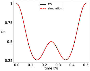
Figure 4: Time-evolution of the IPR $I^{X}_{2}$ during the one-axis twisting protocol for $L=4$ spins-$1/2$. At time $t=0$ the system is prepared with all spins polarized along $x$-direction having IPR is $I^{X}_{2}=1$. At $t=\frac{\pi}{4}$ the GHZ state along $x$-direction is generated, and $I^{X}_{2}=\frac{1}{2}$. The black-solid line ED represents the exact diagonalization results, while the red dashed line corresponds to the results obtained from simulating the quantum algorithm presented in Figure 1.

In Figure 4, we present the OAT dynamics for the case of $L=4$ qubits. In accordance with Eq. (7), the numerical simulation of the quantum algorithm of Figure 1 accurately reproduces the ED curve.

4.2 Probing ergodicity in the extended PXP model

To exemplify the practical utilities of the proposed algorithms, we first implement the algorithm in Figure 2 to investigate the thermalization in a PXP model with Zeeman magnetic field, with Hamiltonian given as:

$$\hat{\mathcal{H}}=\sum_{i=1}^{L}\left(\hat{P}_{i-1}\hat{X}_{i}\hat{P}_{i+1}-h\hat{Z}_{i}\right),$$ (16)

where $\hat{X}_{i},\hat{Z}_{i}$ denotes Pauli-X,Z operators acting on the $i$-th spin, $\hat{P}_{i}$ is the projector on the $\ket{0}$ state of the $i$-th spin, and $h\in[0,1]$ is the amplitude of the external transverse field. We assume periodic boundary conditions. In the absence of the external field, for $h=0$, the PXP model is known as a paradigmatic model of quantum many-body scars [146]. The presence of the scar states is manifested as a lack of thermalization when the system is initialized in particular states, for instance in the Néel state $|0101\cdots\rangle$ [147]. In contrast, for generic initial conditions, the system thermalizes similarly to other interacting non-integrable many-body systems [87]. The quantum many-body scars states form a ladder of highly excited eigenstates extending over the whole spectrum of $\hat{\mathcal{H}}$ [148]. The ground state of the model Eq.(16) undergoes a quantum phase transition of Ising universality class at $h_{c}\approx 0.655$ [149].

The properties of the system in the vicinity of the quantum phase transition in the ground states are linked with the behavior of the quantum many-body scars in [149]. The thermalization of the Néel state under the time evolution generated by Eq.(16) was probed with $\delta\sigma^{z}$ representing the difference between the long-term average of the operator $\hat{Z}$ and the thermal equilibrium expectation value $Z_{\rm th}$:

$$\delta\sigma^{z}=\langle\hat{Z}\rangle-Z_{\rm th}.$$ (17)

The behavior of $\delta\sigma^{z}$ at fixed system size $L$ may be summarized as follows [149]: below the transition, at $h<h_{c}$, lack of thermalization due to the presence of scar states is observed, at the criticality $h\approx h_{c}$ the system thermalizes, while for $h>h_{c}$ lack of thermalization of the system occurs due to a high overlap of the Néel state with the ground state of the system.

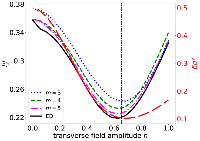
Figure 5: Thermalization and ergodicity breaking in PXP model in the presence of a transverse field $h$, Eq.(16). Left $y$-axis: The IPR $I^{\cal H}_{2}$ in the eigenbasis $\mathcal{B}_{\mathcal{H}}$ of the Hamiltonian is calculated with the algorithm of Figure 2. Simulations are conducted for system size $L=8$, with a fixed $t=1$, and with the number of Trotter steps $N_{t}=10$. The constituent lines (from top to bottom): dotted-blue, dashed-green, dash-dotted-pink, correspond to outcomes obtained by estimation with $m=3,4,5$ ancillary qubits, respectively. The black solid line corresponds to ED results. Rigth red color $y$-axis: long-dashed-red line presents the difference $\delta\sigma^{z}$ between the long-time average and the thermal value of the Pauli-Z operator as a function of the transverse field strength for $L=8$ spins; vertical line corresponds to critical $h_{c}\approx 0.655$  [149].

The thermalization of the system may be also probed by the value of IPR $I^{{\cal H}}_{2}$ of the initial state $|\psi_{0}\rangle=|0101\cdots\rangle$ in the eigenbasis $\mathcal{B}_{\mathcal{H}}$ of the PXP Hamiltonian Eq. (16), equal to the long-time average of the survival probability $|\langle\psi_{0}\ket{\psi(t)}|^{2}$. The results of the algorithm of Figure 2 are presented in Figure 5. We fix $t=1$ and set the number of the Trotter steps as $N_{t}=10$, and compare the obtained value of $I^{{\cal H}}_{2}$ with the exact value of IPR calculated with the exact diagonalization of $\hat{\mathcal{H}}$. As it is expected from Eq. (12), with the increasing number $m=3,4,5$ of the employed ancillary qubits, the results approach the exact diagonalization value [150]. Moreover, the value of IPR decreases monotonically with $h$ in the whole interval $h\lesssim h_{c}$, showing that the thermalization of the system is more effective as the critical regime $h\approx h_{c}$ is approached. At $h\approx h_{c}$, the IPR $I^{{\cal H}}_{2}$ admits a minimal value, and increase at larger $h$, consistently with the behavior of $\delta\sigma^{z}$.

These results show that the proposed algorithm can be useful in probing thermalization and ergodicity breaking in quantum many-body systems.

4.3 IPR for AKLT model

Here, we present an algorithm for obtaining $I_{2}^{Z}$ for the qudit system, with on-site Hilbert space dimension $d=3$. We consider the spin-$1$ chain described by the AKLT (Affleck-Kennedy-Lieb-Tasaki) model [151, 152] with the transverse field and with the open boundary conditions:

$$\hat{\cal H}\!=\!\sum_{i=1}^{L-1}\left[\frac{1}{2}\mathbf{\hat{S}}_{i}\cdot\mathbf{\hat{S}}_{i+1}\!+\!\frac{1}{6}\big{(}\mathbf{\hat{S}}_{i}\cdot\mathbf{\hat{S}}_{i+1}\big{)}^{2}\!+\!\frac{1}{3}\right]-\dfrac{h}{L}\sum^{L}_{i=1}\hat{S}_{i}^{z}.$$ (18)

For $h=0$, the ground state of the Hamiltonian is a valence bond solid where each neighboring site pair is linked by a single valence bond. With open boundary conditions, the edge spins-$1$ have only one neighbor, leaving one of their constituent spin-$1/2$ unpaired (for review see [153]).

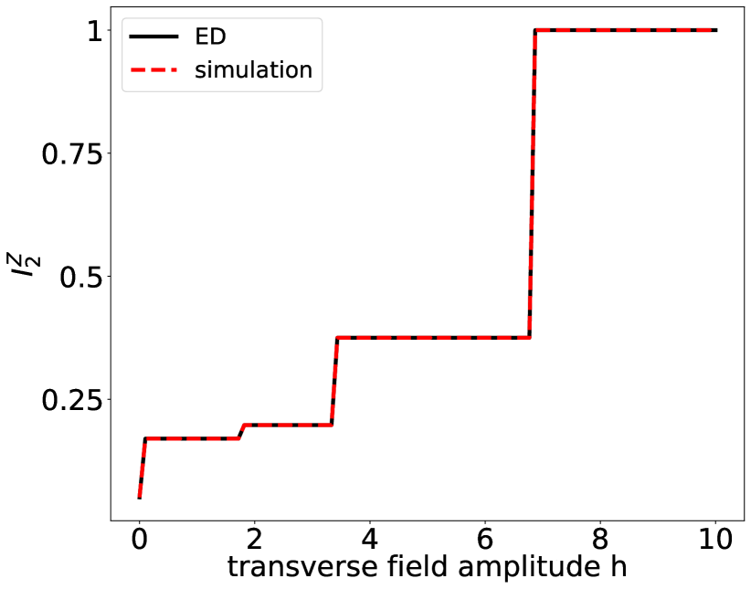
Figure 6: The IPR $I^{Z}_{2}$ of the AKLT ground state, Eq.(18), for $L=4$ spins-$1$, as a function of the transverse field $h$. The black solid line corresponds to ED results, while the red dashed line corresponds to the results of the quantum algorithm in Figure 3.

The AKLT state is a paradigmatic example of a symmetry-protected topological (SPT) order [154]. AKLT states play a role in a measurement-based quantum computation [155, 156, 157], where the computation begins in an appropriately entangled state, such as a g ground state of quantum spin chains with symmetry-protected topological order [158, 159, 160], followed by a set of proper single particle measurements. Recently, it has been shown that the AKLT ground state can be effectively prepared on a quantum circuit [161].

In Figure 6 we present the estimation of $I_{2}^{Z}$ for the ground state of the AKLT model as a function of the transverse field $h$ for a chain of $L=4$ spins-$1$. The results obtained via ED are in perfect agreement with the proposed algorithm, Figure 3. The ground state is perfectly localized $I^{Z}_{2}\to 1$ on a single state of $\mathcal{B}_{Z}$ for $h\gg 1$, and spreads over an increasing number of states $I^{Z}_{2}<1$ of $\mathcal{B}_{Z}$ for smaller values of the transverse field.

5 Conclusion

In this work, we have introduced three quantum algorithms to estimate IPRs and participation entropies of a state of multi-qubit and multi-qudit system. We first focused on a case of a fixed known basis, such the as computational allowing for the estimation of IPRs on quantum devices. The introduced algorithms enable the estimation of IPRs with just single-qubit measurements. We exemplified the utility of the introduced algorithms for non-equilibrium quantum many-body problems by investigating the OAT dynamics. Motivated by the relation of the IPR in the eigenbasis of a given Hamiltonian to the long-time average of survival probability, we introduced a quantum algorithm allowing estimation of the IPR in the Hamiltonian’s eigenbasis without the necessity of the full diagonalization of the Hamiltonian. We have shown that the estimation error diminshes exponentially with the addition of ancillary qubits paralleled by deployment of high powers of the evolution operator. To validate the efficacy of this approach, we conducted simulations of a deformed PXP model. As the number of ancillary qubits increases, the estimated IPR closely aligns with exact diagonalization results, effectively capturing the system’s thermalization properties. Finally, we presented the utilization of our algorithm for multiqudit systems analyzing the ground state of the spin-$1$ AKLT model in the transverse field, showing the perfect agreement between exact results and the proposed algorithm.

In future research, exploring applications of our algorithms in diverse areas such as quantum chemistry, condensed matter physics, and quantum computing optimization tasks could uncover new insights and further validate the effectiveness of quantum simulations in the NISQ era.

6 Acknowledgement

We acknowledge the beneficial discussion with Zhixin Song and Xhek Turkeshi.

ICFO group acknowledges support from: Europea Research Council AdG NOQIA; MCIN/AEI (PGC2018-0910.13039/501100011033,  CEX2019-000910-S/10.13039/501100011033, Plan National FIDEUA PID2019-106901GB-I00, Plan National STAMEENA PID2022-139099NB, I00,project funded by MCIN/AEI/10.13039/501100011033 and by the “European Union NextGenerationEU/PRTR” (PRTR-C17.I1), FPI); QUANTERA MAQS PCI2019-111828-2);  QUANTERA DYNAMITE PCI2022-132919, QuantERA II Programme co-funded by European Union’s Horizon 2020 program under Grant Agreement No 101017733); Ministry for Digital Transformation and of Civil Service of the Spanish Government through the QUANTUM ENIA project call - Quantum Spain project, and by the European Union through the Recovery, Transformation and Resilience Plan - NextGenerationEU within the framework of the Digital Spain 2026 Agenda; Fundació Cellex; Fundació Mir-Puig; Generalitat de Catalunya (European Social Fund FEDER and CERCA program, AGAUR Grant No. 2021 SGR 01452, QuantumCAT  U16-011424, co-funded by ERDF Operational Program of Catalonia 2014-2020); Barcelona Supercomputing Center MareNostrum (FI-2023-1-0013); Funded by the European Union. Views and opinions expressed are however those of the author(s) only and do not necessarily reflect those of the European Union, European Commission, European Climate, Infrastructure and Environment Executive Agency (CINEA), or any other granting authority. Neither the European Union nor any granting authority can be held responsible for them (EU Quantum Flagship PASQuanS2.1, 101113690, EU Horizon 2020 FET-OPEN OPTOlogic, Grant No 899794), EU Horizon Europe Program (This project has received funding from the European Union’s Horizon Europe research and innovation program under grant agreement No 101080086 NeQSTGrant Agreement 101080086 — NeQST); ICFO Internal “QuantumGaudi” project; European Union’s Horizon 2020 program under the Marie Sklodowska-Curie grant agreement No 847648; “La Caixa” Junior Leaders fellowships, La Caixa” Foundation (ID 100010434): CF/BQ/PR23/11980043.

Appendix A Error analysis for $\varepsilon_{r}$ in Sec.3.2

Here we will prove that the error $\epsilon_{r}$ is bounded by $0\leq\epsilon_{r}\leq 4^{-m}\frac{W^{2}}{\Delta^{2}}$. The probability $P_{0,m}$ takes:

$$\begin{split}P_{0,{m}}&=\left<\Psi_{\text{out}}|(|0\right\rangle\left\langle 0|^{\otimes m}\otimes\mathbb{1})|\Psi_{\text{out}}\right\rangle\\ &=\dfrac{1}{4^{m}}\sum_{i,i^{{}^{\prime}},j,j^{{}^{\prime}}}c_{i}c_{j}c^{*}_{i^{\prime}}c^{*}_{j^{\prime}}\sum_{x,x^{\prime}=0}^{2^{m}-1}e^{\text{i}(\tilde{\varepsilon}_{ij}x-\tilde{\varepsilon}_{i^{\prime}j^{\prime}}x^{\prime})t}\langle\varepsilon_{j^{\prime}}|\varepsilon_{j}\rangle\langle\varepsilon_{i^{\prime}}|\varepsilon_{i}\rangle\\ &=\dfrac{1}{4^{m}}\sum_{i,j}|c_{i}|^{2}|c_{j}|^{2}\sum_{x,x^{\prime}=0}^{2^{m}-1}e^{\text{i}\tilde{\varepsilon}_{ij}(x-x^{\prime})t}\\ &=\sum_{i}|c_{i}|^{4}+\dfrac{1}{4^{m}}\sum_{i\neq j}|c_{i}|^{2}|c_{j}|^{2}\sum_{x,x^{\prime}=0}^{2^{m}-1}e^{\text{i}\tilde{\varepsilon}_{ij}(x-x^{\prime})t},\end{split}$$

here the first term is $I^{\mathcal{H}}_{2}$, and the second term is $\epsilon_{r}$ in Eq. (12). Further simplification leads to:

$$\begin{split}\epsilon_{r}&=\dfrac{1}{4^{m}}\sum_{i\neq j}|c_{i}|^{2}|c_{j}|^{2}\sum_{x,x^{\prime}=0}^{2^{m}-1}e^{\text{i}\tilde{\varepsilon}_{ij}(x-x^{\prime})t}\\ &=\dfrac{1}{4^{m}}\sum_{i\neq j}|c_{i}|^{2}|c_{j}|^{2}\sum_{x=0}^{2^{m}-1}e^{\text{i}\tilde{\varepsilon}_{ij}xt}\sum_{x^{\prime}=0}^{2^{m}-1}e^{\text{i}\tilde{\varepsilon}_{ij}x^{\prime}t}\\ &=\dfrac{1}{4^{m}}\sum_{i\neq j}|c_{i}|^{2}|c_{j}|^{2}\big{(}\dfrac{1-e^{\text{i}\tilde{\varepsilon}_{ij}2^{m}t}}{1-e^{\text{i}\tilde{\varepsilon}_{ij}t}}\big{)}\big{(}\dfrac{1-e^{-\text{i}\tilde{\varepsilon}_{ij}2^{m}t}}{1-e^{-\text{i}\tilde{\varepsilon}_{ij}t}}\big{)}\\ &=\dfrac{1}{4^{m}}\sum_{i\neq j}|c_{i}|^{2}|c_{j}|^{2}\dfrac{1-\cos{(2^{m}\tilde{\varepsilon}_{ij}t})}{1-\cos{(\tilde{\varepsilon}_{ij}t)}}.\end{split}$$

For any real $\theta$, $1-\cos\theta\leq 2$, so $\epsilon_{r}\leq\dfrac{1}{4^{m}}\sum_{i\neq j}|c_{i}|^{2}|c_{j}|^{2}\dfrac{2}{1-\cos{(\tilde{\varepsilon}_{ij}t)}}$. The inequality above can be further bounded when $|\tilde{\varepsilon}_{ij}t|\in(0,\pi],\forall i\neq j$ since $1-\cos\theta\geq\frac{2\theta^{2}}{\pi^{2}}$ for $\theta\in[-\pi,\pi]$:

$$\begin{split}\epsilon_{r}&\leq\dfrac{1}{4^{m}}\sum_{ij}|c_{i}|^{2}|c_{j}|^{2}\dfrac{\pi^{2}}{\tilde{\varepsilon}_{ij}^{2}t^{2}}\leq\dfrac{1}{4^{m}}\sum_{ij}|c_{i}|^{2}|c_{j}|^{2}\dfrac{\pi^{2}}{(\varepsilon_{i}-\varepsilon_{j})^{2}t^{2}}\\ &\leq\dfrac{1}{4^{m}}\sum_{ij}|c_{i}|^{2}|c_{j}|^{2}\dfrac{\pi^{2}}{\Delta^{2}t^{2}}\leq 4^{-m}\dfrac{\pi^{2}}{\Delta^{2}t^{2}}.\end{split}$$

Apparently, $\epsilon_{r}\geq 0$, then we finish the proof of $0\leq\epsilon_{r}\leq 4^{-m}\frac{\pi^{2}}{\Delta^{2}t^{2}}$.

Appendix B OAT experiment on IBM quantum machine

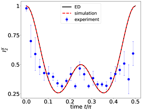
Figure 7: Time evolution of the IPR $I^{X}_{2}$ for the OAT model, Sec.4.1. The blue markers with error bars present the experiments run on ibm$\_$torino backend at IBM quantum platform, [162], by executing the quantum algorithm Figure 1 after averaging over $5$ runs at each time-stamp.

Here, we present an experimental realization of a quantum algorithm, as shown in Figure  1, conducted on an IBM quantum machine. This involves measuring the IPR $I^{X}_{z}$ for the one-axis twisting protocol, detailed in Section 4.1.

In Figure 7, the blue markers with error bars represent the estimated values of $I^{X}_{2}$. These estimations qualitatively align with the exact diagonalization (ED) results, depicted by the black solid line, and with the numerical simulations of the algorithm, indicated by the red dashed line. The experiment was conducted on IBM’s ibm_torino platform, with each data point derived from 2048 measurement shots per time step. We implemented noise mitigation strategies, including dynamical decoupling, and optimized the circuit transpilation as described in [162].

Transpiling the quantum algorithm from Figure 1 into native quantum gates notably increases the circuit depth. The individual outliers observed in Figure 7 are linked to instances where transpilation at certain time splits ($t$) produced circuits significantly deeper than others, thereby heightening their susceptibility to noise. At $t=0$, where the evolution is not executed, the overhead from gates is equivalent to that of an idle gate, which results in a more precise measurement outcome. For further details on the numerical implementation, please refer to the GitHub repository cited in [150].

The experimentally obtained value of $I^{X}_{2}\approx\frac{1}{2}$ at $t\approx\pi/4$ substantiates the efficacy of the introduced quantum algorithm for exploring many-body dynamics on future fault-tolerant quantum computers.

References

- [1] Luigi Amico, Rosario Fazio, Andreas Osterloh, and Vlatko Vedral. “Entanglement in many-body systems”. Rev. Mod. Phys. 80, 517–576 (2008).
- [2] J. Eisert, M. Cramer, and M. B. Plenio. “Colloquium: Area laws for the entanglement entropy”. Rev. Mod. Phys. 82, 277–306 (2010).
- [3] Ulrich Schollwöck. “The density-matrix renormalization group in the age of matrix product states”. Annals of Physics 326, 96–192 (2011).
- [4] Álvaro M. Alhambra. “Quantum many-body systems in thermal equilibrium”. PRX Quantum 4, 040201 (2023).
- [5] Jens Eisert, Mathis Friesdorf, and Christian Gogolin. “Quantum many-body systems out of equilibrium”. Nature Physics 11, 124–130 (2015).
- [6] Luca D’Alessio, Yariv Kafri, Anatoli Polkovnikov, and Marcos Rigol. “From quantum chaos and eigenstate thermalization to statistical mechanics and thermodynamics”. Advances in Physics 65, 239–362 (2016).
- [7] B. Bertini, F. Heidrich-Meisner, C. Karrasch, T. Prosen, R. Steinigeweg, and M. Žnidarič. “Finite-temperature transport in one-dimensional quantum lattice models”. Rev. Mod. Phys. 93, 025003 (2021).
- [8] Dmitry A. Abanin, Ehud Altman, Immanuel Bloch, and Maksym Serbyn. “Colloquium: Many-body localization, thermalization, and entanglement”. Rev. Mod. Phys. 91, 021001 (2019).
- [9] Matthew P.A. Fisher, Vedika Khemani, Adam Nahum, and Sagar Vijay. “Random quantum circuits”. Annual Review of Condensed Matter Physics 14, 335–379 (2023).
- [10] Piotr Sierant, Maciej Lewenstein, Antonello Scardicchio, Lev Vidmar, and Jakub Zakrzewski. “Many-body localization in the age of classical computing” (2024). arXiv:2403.07111.
- [11] Philip W Anderson. “More is different: Broken symmetry and the nature of the hierarchical structure of science.”. Science 177, 393–396 (1972).
- [12] Maciej Lewenstein, Anna Sanpera, Veronica Ahufinger, Bogdan Damski, Aditi Sen(De), and Ujjwal Sen. “Ultracold atomic gases in optical lattices: mimicking condensed matter physics and beyond”. Advances in Physics 56, 243–379 (2007).
- [13] Christian Gross and Immanuel Bloch. “Quantum simulations with ultracold atoms in optical lattices”. Science 357, 995–1001 (2017).
- [14] Antoine Browaeys and Thierry Lahaye. “Many-body physics with individually controlled rydberg atoms”. Nature Physics 16, 132–142 (2020).
- [15] Joana Fraxanet, Tymoteusz Salamon, and Maciej Lewenstein. “The coming decades of quantum simulation”. Pages 85–125. Springer International Publishing. Cham (2023).
- [16] Richard P Feynman. “Simulating physics with computers”. International Journal of Theoretical Physics21 (1982).
- [17] Frank Arute, Kunal Arya, Ryan Babbush, Dave Bacon, Joseph C Bardin, Rami Barends, Rupak Biswas, Sergio Boixo, Fernando GSL Brandao, David A Buell, et al. “Quantum supremacy using a programmable superconducting processor”. Nature 574, 505 (2019). url: https://doi.org/10.1038/s41586-019-1666-5.
- [18] Yulin Wu, Wan-Su Bao, Sirui Cao, Fusheng Chen, Ming-Cheng Chen, Xiawei Chen, Tung-Hsun Chung, Hui Deng, and Yajie et al Du. “Strong quantum computational advantage using a superconducting quantum processor”. Phys. Rev. Lett. 127, 180501 (2021).
- [19] Youngseok Kim, Andrew Eddins, Sajant Anand, Ken Xuan Wei, Ewout van den Berg, Sami Rosenblatt, Hasan Nayfeh, Yantao Wu, Michael Zaletel, Kristan Temme, and Abhinav Kandala. “Evidence for the utility of quantum computing before fault tolerance”. Nature 618, 500–505 (2023).
- [20] John Preskill. “Quantum computing in the nisq era and beyond”. Quantum 2, 79 (2018).
- [21] P.W. Shor. “Algorithms for quantum computation: discrete logarithms and factoring”. In Proceedings 35th Annual Symposium on Foundations of Computer Science. Pages 124–134. (1994).
- [22] Lov K. Grover. “A fast quantum mechanical algorithm for database search” (1996). arXiv:quant-ph/9605043.
- [23] A Yu Kitaev. “Quantum measurements and the abelian stabilizer problem” (1995).
- [24] Ashley Montanaro. “Quantum algorithms: an overview”. npj Quantum Information 2, 15023 (2016).
- [25] Kishor Bharti, Alba Cervera-Lierta, Thi Ha Kyaw, Tobias Haug, Sumner Alperin-Lea, Abhinav Anand, Matthias Degroote, Hermanni Heimonen, Jakob S. Kottmann, Tim Menke, Wai-Keong Mok, Sukin Sim, Leong-Chuan Kwek, and Alán Aspuru-Guzik. “Noisy intermediate-scale quantum algorithms”. Rev. Mod. Phys. 94, 015004 (2022).
- [26] Alexander Miessen, Pauline J Ollitrault, and Ivano Tavernelli. “Quantum algorithms for quantum dynamics: A performance study on the spin-boson model”. Physical Review Research 3, 043212 (2021).
- [27] Alexander Miessen, Pauline J Ollitrault, Francesco Tacchino, and Ivano Tavernelli. “Quantum algorithms for quantum dynamics”. Nature Computational Science 3, 25–37 (2023).
- [28] Christof Zalka. “Efficient simulation of quantum systems by quantum computers”. Fortschritte der Physik: Progress of Physics 46, 877–879 (1998).
- [29] Richard Cleve and Chunhao Wang. “Efficient quantum algorithms for simulating lindblad evolution” (2019). arXiv:1612.09512.
- [30] Alán Aspuru-Guzik, Anthony D Dutoi, Peter J Love, and Martin Head-Gordon. “Simulated quantum computation of molecular energies”. Science 309, 1704–1707 (2005).
- [31] Hefeng Wang, Sabre Kais, Alán Aspuru-Guzik, and Mark R. Hoffmann. “Quantum algorithm for obtaining the energy spectrum of molecular systems”. Physical Chemistry Chemical Physics 10, 5388 (2008).
- [32] Xiaoyang Wang, Xu Feng, Tobias Hartung, Karl Jansen, and Paolo Stornati. “Critical behavior of the ising model by preparing the thermal state on a quantum computer”. Phys. Rev. A 108, 022612 (2023).
- [33] David Poulin and Pawel Wocjan. “Sampling from the thermal quantum gibbs state and evaluating partition functions with a quantum computer”. Phys. Rev. Lett. 103, 220502 (2009).
- [34] Youle Wang, Guangxi Li, and Xin Wang. “Variational quantum gibbs state preparation with a truncated taylor series”. Physical Review Applied 16, 054035 (2021).
- [35] Tyson Jones, Suguru Endo, Sam McArdle, Xiao Yuan, and Simon C Benjamin. “Variational quantum algorithms for discovering hamiltonian spectra”. Physical Review A 99, 062304 (2019).
- [36] Jacob Smith, Aaron Lee, Philip Richerme, Brian Neyenhuis, Paul W Hess, Philipp Hauke, Markus Heyl, David A Huse, and Christopher Monroe. “Many-body localization in a quantum simulator with programmable random disorder”. Nature Physics 12, 907–911 (2016).
- [37] I-Chi Chen, Benjamin Burdick, Yongxin Yao, Peter P Orth, and Thomas Iadecola. “Error-mitigated simulation of quantum many-body scars on quantum computers with pulse-level control”. Physical Review Research 4, 043027 (2022).
- [38] Shuo Liu, Shi-Xin Zhang, Chang-Yu Hsieh, Shengyu Zhang, and Hong Yao. “Probing many-body localization by excited-state variational quantum eigensolver”. Physical Review B 107, 024204 (2023).
- [39] Bárbara Andrade, Utso Bhattacharya, Ravindra W. Chhajlany, Tobias Graß, and Maciej Lewenstein. “Observing quantum many-body scars in random quantum circuits” (2024). arXiv:2402.06489.
- [40] Alexander J McCaskey, Zachary P Parks, Jacek Jakowski, Shirley V Moore, Titus D Morris, Travis S Humble, and Raphael C Pooser. “Quantum chemistry as a benchmark for near-term quantum computers”. npj Quantum Information 5, 99 (2019).
- [41] Abhinav Kandala, Antonio Mezzacapo, Kristan Temme, Maika Takita, Markus Brink, Jerry M Chow, and Jay M Gambetta. “Hardware-efficient variational quantum eigensolver for small molecules and quantum magnets”. nature 549, 242–246 (2017).
- [42] Edward Farhi, Jeffrey Goldstone, and Sam Gutmann. “A quantum approximate optimization algorithm” (2014).
- [43] M. Cerezo, Andrew Arrasmith, Ryan Babbush, Simon C. Benjamin, Suguru Endo, Keisuke Fujii, Jarrod R. McClean, Kosuke Mitarai, Xiao Yuan, Lukasz Cincio, and Patrick J. Coles. “Variational quantum algorithms”. Nature Reviews Physics 3, 625–644 (2021).
- [44] Anna Dawid, Julian Arnold, Borja Requena, Alexander Gresch, Marcin Płodzień, Kaelan Donatella, Kim A. Nicoli, Paolo Stornati, Rouven Koch, Miriam Büttner, Robert Okuła, Gorka Muñoz-Gil, Rodrigo A. Vargas-Hernández, Alba Cervera-Lierta, Juan Carrasquilla, Vedran Dunjko, Marylou Gabrié, Patrick Huembeli, Evert van Nieuwenburg, Filippo Vicentini, Lei Wang, Sebastian J. Wetzel, Giuseppe Carleo, Eliška Greplová, Roman Krems, Florian Marquardt, Michał Tomza, Maciej Lewenstein, and Alexandre Dauphin. “Modern applications of machine learning in quantum sciences” (2023). arXiv:2204.04198.
- [45] K. Vogel and H. Risken. “Determination of quasiprobability distributions in terms of probability distributions for the rotated quadrature phase”. Phys. Rev. A 40, 2847–2849 (1989).
- [46] Marcus Cramer, Martin B. Plenio, Steven T. Flammia, Rolando Somma, David Gross, Stephen D. Bartlett, Olivier Landon-Cardinal, David Poulin, and Yi-Kai Liu. “Efficient quantum state tomography”. Nature Communications 1, 149 (2010).
- [47] Hsin-Yuan Huang, Richard Kueng, and John Preskill. “Predicting many properties of a quantum system from very few measurements”. Nature Physics 16, 1050–1057 (2020).
- [48] Andreas Elben, Steven T. Flammia, Hsin-Yuan Huang, Richard Kueng, John Preskill, Benoît Vermersch, and Peter Zoller. “The randomized measurement toolbox”. Nature Reviews Physics 5, 9–24 (2023).
- [49] JS Pedernales, R Di Candia, IL Egusquiza, J Casanova, and Enrique Solano. “Efficient quantum algorithm for computing n-time correlation functions”. Physical Review Letters 113, 020505 (2014).
- [50] Sonika Johri, Damian S Steiger, and Matthias Troyer. “Entanglement spectroscopy on a quantum computer”. Physical Review B 96, 195136 (2017).
- [51] M. Dalmonte, B. Vermersch, and P. Zoller. “Quantum simulation and spectroscopy of entanglement hamiltonians”. Nature Physics 14, 827–831 (2018).
- [52] Tiff Brydges, Andreas Elben, Petar Jurcevic, Benoît Vermersch, Christine Maier, Ben P. Lanyon, Peter Zoller, Rainer Blatt, and Christian F. Roos. “Probing rényi entanglement entropy via randomized measurements”. Science 364, 260–263 (2019). arXiv:https://www.science.org/doi/pdf/10.1126/science.aau4963.
- [53] Youle Wang, Benchi Zhao, and Xin Wang. “Quantum algorithms for estimating quantum entropies”. Physical Review Applied 19, 044041 (2023).
- [54] Martin Gärttner, Justin G Bohnet, Arghavan Safavi-Naini, Michael L Wall, John J Bollinger, and Ana Maria Rey. “Measuring out-of-time-order correlations and multiple quantum spectra in a trapped-ion quantum magnet”. Nature Physics 13, 781–786 (2017).
- [55] Xiao Mi, Pedram Roushan, Chris Quintana, Salvatore Mandra, Jeffrey Marshall, Charles Neill, Frank Arute, Kunal Arya, Juan Atalaya, Ryan Babbush, et al. “Information scrambling in quantum circuits”. Science 374, 1479–1483 (2021).
- [56] Tobias Haug, Soovin Lee, and M. S. Kim. “Efficient stabilizer entropies for quantum computers” (2023). arXiv:2305.19152.
- [57] Lorenzo Leone, Salvatore F. E. Oliviero, and Alioscia Hamma. “Stabilizer rényi entropy”. Phys. Rev. Lett. 128, 050402 (2022).
- [58] D.J. Thouless. “Electrons in disordered systems and the theory of localization”. Physics Reports 13, 93 – 142 (1974).
- [59] B Kramer and A MacKinnon. “Localization: theory and experiment”. Reports on Progress in Physics 56, 1469 (1993).
- [60] Ferdinand Evers and Alexander D. Mirlin. “Anderson transitions”. Rev. Mod. Phys. 80, 1355–1417 (2008).
- [61] Alberto Rodriguez, Louella J. Vasquez, and Rudolf A. Römer. “Multifractal analysis with the probability density function at the three-dimensional anderson transition”. Phys. Rev. Lett. 102, 106406 (2009).
- [62] Alberto Rodriguez, Louella J. Vasquez, Keith Slevin, and Rudolf A. Römer. “Critical parameters from a generalized multifractal analysis at the anderson transition”. Phys. Rev. Lett. 105, 046403 (2010).
- [63] K. S. Tikhonov, A. D. Mirlin, and M. A. Skvortsov. “Anderson localization and ergodicity on random regular graphs”. Phys. Rev. B 94, 220203 (2016).
- [64] K. S. Tikhonov and A. D. Mirlin. “Fractality of wave functions on a cayley tree: Difference between tree and locally treelike graph without boundary”. Phys. Rev. B 94, 184203 (2016).
- [65] K. S. Tikhonov and A. D. Mirlin. “Statistics of eigenstates near the localization transition on random regular graphs”. Phys. Rev. B 99, 024202 (2019).
- [66] M. Pino. “Scaling up the anderson transition in random-regular graphs”. Phys. Rev. Res. 2, 042031 (2020).
- [67] Carlo Vanoni, Boris L. Altshuler, Vladimir E. Kravtsov, and Antonello Scardicchio. “Renormalization group analysis of the anderson model on random regular graphs” (2023). arXiv:2306.14965.
- [68] I. García-Mata, J. Martin, O. Giraud, B. Georgeot, R. Dubertrand, and G. Lemarié. “Critical properties of the Anderson transition on random graphs: Two-parameter scaling theory, Kosterlitz-Thouless type flow, and many-body localization”. Phys. Rev. B 106, 214202 (2022).
- [69] Piotr Sierant, Maciej Lewenstein, and Antonello Scardicchio. “Universality in Anderson localization on random graphs with varying connectivity”. SciPost Phys. 15, 045 (2023).
- [70] Carlo Vanoni and Vittorio Vitale. “An analysis of localization transitions using non-parametric unsupervised learning” (2024). arXiv:2311.16050.
- [71] Thomas C Halsey, Mogens H Jensen, Leo P Kadanoff, Itamar Procaccia, and Boris I Shraiman. “Fractal measures and their singularities: The characterization of strange sets”. Physical review A 33, 1141 (1986).
- [72] Arnd Bäcker, Masudul Haque, and Ivan M. Khaymovich. “Multifractal dimensions for random matrices, chaotic quantum maps, and many-body systems”. Phys. Rev. E 100, 032117 (2019).
- [73] H. Eugene Stanley and Paul Meakin. “Multifractal phenomena in physics and chemistry”. Nature 335, 405–409 (1988).
- [74] Marlena Dziurawiec, Jessica O. de Almeida, Mohit Lal Bera, Marcin Płodzień, Maciej M. Maśka, Maciej Lewenstein, Tobias Grass, and Utso Bhattacharya. “Unraveling multifractality and mobility edges in quasiperiodic aubry-andré-harper chains through high-harmonic generation” (2023). arXiv:2310.02757.
- [75] Jean-Marie Stéphan, Shunsuke Furukawa, Grégoire Misguich, and Vincent Pasquier. “Shannon and entanglement entropies of one- and two-dimensional critical wave functions”. Phys. Rev. B 80, 184421 (2009).
- [76] J.-M. Stéphan, G. Misguich, and V. Pasquier. “Rényi entropy of a line in two-dimensional ising models”. Phys. Rev. B 82, 125455 (2010).
- [77] Jean-Marie Stéphan. “Shannon and rényi mutual information in quantum critical spin chains”. Phys. Rev. B 90, 045424 (2014).
- [78] David J. Luitz, Fabien Alet, and Nicolas Laflorencie. “Universal behavior beyond multifractality in quantum many-body systems”. Phys. Rev. Lett. 112, 057203 (2014).
- [79] David J. Luitz, Xavier Plat, Nicolas Laflorencie, and Fabien Alet. “Improving entanglement and thermodynamic rényi entropy measurements in quantum monte carlo”. Phys. Rev. B 90, 125105 (2014).
- [80] M. Pino, V. E. Kravtsov, B. L. Altshuler, and L. B. Ioffe. “Multifractal metal in a disordered josephson junctions array”. Phys. Rev. B 96, 214205 (2017).
- [81] Jakob Lindinger, Andreas Buchleitner, and Alberto Rodríguez. “Many-body multifractality throughout bosonic superfluid and mott insulator phases”. Phys. Rev. Lett. 122, 106603 (2019).
- [82] Lukas Pausch, Edoardo G. Carnio, Alberto Rodríguez, and Andreas Buchleitner. “Chaos and ergodicity across the energy spectrum of interacting bosons”. Phys. Rev. Lett. 126, 150601 (2021).
- [83] Philipp Frey, David Mikhail, Stephan Rachel, and Lucas Hackl. “Probing hilbert space fragmentation and the block inverse participation ratio”. Phys. Rev. B 109, 064302 (2024).
- [84] A De Luca and A Scardicchio. “Ergodicity breaking in a model showing many-body localization”. EPL (Europhysics Letters) 101, 37003 (2013).
- [85] Mark Srednicki. “Chaos and quantum thermalization”. Phys. Rev. E 50, 888–901 (1994).
- [86] J. M. Deutsch. “Quantum statistical mechanics in a closed system”. Phys. Rev. A 43, 2046–2049 (1991).
- [87] Marcos Rigol, Vanja Dunjko, and Maxim Olshanii. “Thermalization and its mechanism for generic isolated quantum systems”. Nature 452, 854 EP – (2008). url: https://doi.org/10.1038/nature06838.
- [88] Silvia Pappalardi, Laura Foini, and Jorge Kurchan. “Eigenstate thermalization hypothesis and free probability”. Phys. Rev. Lett. 129, 170603 (2022).
- [89] Michele Fava, Jorge Kurchan, and Silvia Pappalardi. “Designs via free probability” (2023). arXiv:2308.06200.
- [90] Rahul Nandkishore and David A. Huse. “Many-Body Localization and Thermalization in Quantum Statistical Mechanics”. Annual Review of Condensed Matter Physics 6, 15–38 (2015).
- [91] Fabien Alet and Nicolas Laflorencie. “Many-body localization: An introduction and selected topics”. Comptes Rendus Physique 19, 498–525 (2018).
- [92] Nicolas Macé, Fabien Alet, and Nicolas Laflorencie. “Multifractal scalings across the many-body localization transition”. Phys. Rev. Lett. 123, 180601 (2019).
- [93] Piotr Sierant and Xhek Turkeshi. “Universal behavior beyond multifractality of wave functions at measurement-induced phase transitions”. Physical Review Letters 128, 130605 (2022).
- [94] Piotr Sierant, Marco Schirò, Maciej Lewenstein, and Xhek Turkeshi. “Measurement-induced phase transitions in -dimensional stabilizer circuits”. Phys. Rev. B 106, 214316 (2022).
- [95] Xhek Turkeshi and Piotr Sierant. “Hilbert space delocalization under random unitary circuits” (2024). arXiv:2404.10725.
- [96] T. Baumgratz, M. Cramer, and M. B. Plenio. “Quantifying coherence”. Phys. Rev. Lett. 113, 140401 (2014).
- [97] Eric Chitambar and Gilad Gour. “Quantum resource theories”. Rev. Mod. Phys. 91, 025001 (2019).
- [98] Xhek Turkeshi, Marco Schirò, and Piotr Sierant. “Measuring nonstabilizerness via multifractal flatness”. Phys. Rev. A 108, 042408 (2023).
- [99] Scott Aaronson and Alex Arkhipov. “The computational complexity of linear optics”. In Proceedings of the forty-third annual ACM symposium on Theory of computing. Pages 333–342. ACM (2011).
- [100] Michael J. Bremner, Ashley Montanaro, and Dan J. Shepherd. “Average-case complexity versus approximate simulation of commuting quantum computations”. Phys. Rev. Lett. 117, 080501 (2016).
- [101] Adam Bouland, Bill Fefferman, Chinmay Nirkhe, and Umesh Vazirani. “On the complexity and verification of quantum random circuit sampling”. Nature Physics 15, 159–163 (2019).
- [102] Michał Oszmaniec, Ninnat Dangniam, Mauro E.S. Morales, and Zoltán Zimborás. “Fermion sampling: A robust quantum computational advantage scheme using fermionic linear optics and magic input states”. PRX Quantum 3, 020328 (2022).
- [103] Sergio Boixo, Sergei V. Isakov, Vadim N. Smelyanskiy, Ryan Babbush, Nan Ding, Zhang Jiang, Michael J. Bremner, John M. Martinis, and Hartmut Neven. “Characterizing quantum supremacy in near-term devices”. Nature Physics 14, 595–600 (2018).
- [104] Gilles Brassard, Peter Hoyer, Michele Mosca, and Alain Tapp. “Quantum amplitude amplification and estimation”. Contemporary Mathematics 305, 53–74 (2002).
- [105] Harry Buhrman, Richard Cleve, John Watrous, and Ronald De Wolf. “Quantum fingerprinting”. Physical Review Letters 87, 167902 (2001).
- [106] E. J. Torres-Herrera and Lea F. Santos. “Dynamics at the many-body localization transition”. Phys. Rev. B 92, 014208 (2015).
- [107] E. J. Torres-Herrera, Antonio M. García-García, and Lea F. Santos. “Generic dynamical features of quenched interacting quantum systems: Survival probability, density imbalance, and out-of-time-ordered correlator”. Phys. Rev. B 97, 060303 (2018).
- [108] P. Prelovšek, O. S. Barišić, and M. Mierzejewski. “Reduced-basis approach to many-body localization”. Phys. Rev. B 97, 035104 (2018).
- [109] K. S. Tikhonov and A. D. Mirlin. “Many-body localization transition with power-law interactions: Statistics of eigenstates”. Phys. Rev. B 97, 214205 (2018).
- [110] Mauro Schiulaz, E. Jonathan Torres-Herrera, and Lea F. Santos. “Thouless and relaxation time scales in many-body quantum systems”. Phys. Rev. B 99, 174313 (2019).
- [111] Lea F. Santos, Francisco Pérez-Bernal, and E. Jonathan Torres-Herrera. “Speck of chaos”. Phys. Rev. Res. 2, 043034 (2020).
- [112] Miroslav Hopjan and Lev Vidmar. “Scale-invariant survival probability at eigenstate transitions”. Phys. Rev. Lett. 131, 060404 (2023).
- [113] Bikram Pain, Kritika Khanwal, and Sthitadhi Roy. “Connection between Hilbert-space return probability and real-space autocorrelations in quantum spin chains”. Phys. Rev. B 108, L140201 (2023).
- [114] Isabel Creed, David E. Logan, and Sthitadhi Roy. “Probability transport on the fock space of a disordered quantum spin chain”. Phys. Rev. B 107, 094206 (2023).
- [115] Don Coppersmith. “An approximate fourier transform useful in quantum factoring” (2002).
- [116] Michael A Nielsen and Isaac L Chuang. “Quantum computation and quantum information”. Phys. Today 54, 60 (2001).
- [117] Hale F Trotter. “On the product of semi-groups of operators”. Proceedings of the American Mathematical Society 10, 545–551 (1959).
- [118] Masuo Suzuki. “Generalized trotter’s formula and systematic approximants of exponential operators and inner derivations with applications to many-body problems”. Communications in Mathematical Physics 51, 183–190 (1976).
- [119] Seth Lloyd. “Universal quantum simulators”. Science 273, 1073–1078 (1996).
- [120] Pavel Hrmo, Benjamin Wilhelm, Lukas Gerster, Martin W. van Mourik, Marcus Huber, Rainer Blatt, Philipp Schindler, Thomas Monz, and Martin Ringbauer. “Native qudit entanglement in a trapped ion quantum processor”. Nature Communications 14, 2242 (2023).
- [121] Noah Goss, Alexis Morvan, Brian Marinelli, Bradley K. Mitchell, Long B. Nguyen, Ravi K. Naik, Larry Chen, Christian Jünger, John Mark Kreikebaum, David I. Santiago, Joel J. Wallman, and Irfan Siddiqi. “High-fidelity qutrit entangling gates for superconducting circuits”. Nature Communications 13, 7481 (2022).
- [122] Martin Ringbauer, Michael Meth, Lukas Postler, Roman Stricker, Rainer Blatt, Philipp Schindler, and Thomas Monz. “A universal qudit quantum processor with trapped ions”. Nature Physics 18, 1053–1057 (2022).
- [123] L. Funcke, T. Hartung, K. Jansen, S. Kühn, M. Schneider, P. Stornati, and X. Wang. “Towards quantum simulations in particle physics and beyond on noisy intermediate-scale quantum devices”. Philosophical Transactions of the Royal Society A: Mathematical, Physical and Engineering Sciences380 (2021).
- [124] Alberto Di Meglio, Karl Jansen, Ivano Tavernelli, Constantia Alexandrou, Srinivasan Arunachalam, Christian W. Bauer, Kerstin Borras, Stefano Carrazza, Arianna Crippa, Vincent Croft, Roland de Putter, Andrea Delgado, Vedran Dunjko, Daniel J. Egger, Elias Fernandez-Combarro, Elina Fuchs, Lena Funcke, Daniel Gonzalez-Cuadra, Michele Grossi, Jad C. Halimeh, Zoe Holmes, Stefan Kuhn, Denis Lacroix, Randy Lewis, Donatella Lucchesi, Miriam Lucio Martinez, Federico Meloni, Antonio Mezzacapo, Simone Montangero, Lento Nagano, Voica Radescu, Enrique Rico Ortega, Alessandro Roggero, Julian Schuhmacher, Joao Seixas, Pietro Silvi, Panagiotis Spentzouris, Francesco Tacchino, Kristan Temme, Koji Terashi, Jordi Tura, Cenk Tuysuz, Sofia Vallecorsa, Uwe-Jens Wiese, Shinjae Yoo, and Jinglei Zhang. “Quantum computing for high-energy physics: State of the art and challenges. summary of the qc4hep working group” (2023). arXiv:2307.03236.
- [125] Christian W. Bauer, Zohreh Davoudi, A. Baha Balantekin, Tanmoy Bhattacharya, Marcela Carena, Wibe A. de Jong, Patrick Draper, Aida El-Khadra, Nate Gemelke, Masanori Hanada, Dmitri Kharzeev, Henry Lamm, Ying-Ying Li, Junyu Liu, Mikhail Lukin, Yannick Meurice, Christopher Monroe, Benjamin Nachman, Guido Pagano, John Preskill, Enrico Rinaldi, Alessandro Roggero, David I. Santiago, Martin J. Savage, Irfan Siddiqi, George Siopsis, David Van Zanten, Nathan Wiebe, Yukari Yamauchi, Kübra Yeter-Aydeniz, and Silvia Zorzetti. “Quantum simulation for high-energy physics”. PRX Quantum 4, 027001 (2023).
- [126] Yuchen Wang, Zixuan Hu, Barry C Sanders, and Sabre Kais. “Qudits and high-dimensional quantum computing”. Frontiers in Physics 8, 589504 (2020).
- [127] Masahiro Kitagawa and Masahito Ueda. “Squeezed spin states”. Physical Review A 47, 5138 (1993).
- [128] David J Wineland, John J Bollinger, Wayne M Itano, and DJ Heinzen. “Squeezed atomic states and projection noise in spectroscopy”. Physical Review A 50, 67 (1994).
- [129] Luca Pezze, Augusto Smerzi, Markus K Oberthaler, Roman Schmied, and Philipp Treutlein. “Quantum metrology with nonclassical states of atomic ensembles”. Reviews of Modern Physics 90, 035005 (2018).
- [130] Florian Wolfgramm, Alessandro Cere, Federica A Beduini, Ana Predojević, Marco Koschorreck, and Morgan W Mitchell. “Squeezed-light optical magnetometry”. Physical review letters 105, 053601 (2010).
- [131] Guillem Müller-Rigat, Anubhav Kumar Srivastava, Stanisław Kurdziałek, Grzegorz Rajchel-Mieldzioć, Maciej Lewenstein, and Irénée Frérot. “Certifying the quantum fisher information from a given set of mean values: a semidefinite programming approach”. Quantum 7, 1152 (2023).
- [132] Roman Schmied, Jean-Daniel Bancal, Baptiste Allard, Matteo Fadel, Valerio Scarani, Philipp Treutlein, and Nicolas Sangouard. “Bell correlations in a bose-einstein condensate”. Science 352, 441–444 (2016).
- [133] Flavio Baccari, Jordi Tura, Matteo Fadel, Albert Aloy, J-D Bancal, Nicolas Sangouard, Maciej Lewenstein, Antonio Acín, and Remigiusz Augusiak. “Bell correlation depth in many-body systems”. Physical Review A 100, 022121 (2019).
- [134] Jordi Tura, Remigiusz Augusiak, Ana Belén Sainz, Tamas Vértesi, Maciej Lewenstein, and Antonio Acín. “Detecting nonlocality in many-body quantum states”. Science 344, 1256–1258 (2014).
- [135] A. Aloy, J. Tura, F. Baccari, A. Acín, M. Lewenstein, and R. Augusiak. “Device-independent witnesses of entanglement depth from two-body correlators”. Phys. Rev. Lett. 123, 100507 (2019).
- [136] Guillem Müller-Rigat, Albert Aloy, Maciej Lewenstein, and Irénée Frérot. “Inferring nonlinear many-body bell inequalities from average two-body correlations: Systematic approach for arbitrary spin- ensembles”. PRX Quantum 2, 030329 (2021).
- [137] Artur Niezgoda, Miłosz Panfil, and Jan Chwedeńczuk. “Quantum correlations in spin chains”. Phys. Rev. A 102, 042206 (2020).
- [138] Artur Niezgoda and Jan Chwedeńczuk. “Many-body nonlocality as a resource for quantum-enhanced metrology”. Phys. Rev. Lett. 126, 210506 (2021).
- [139] Marcin Płodzień, Maciej Kościelski, Emilia Witkowska, and Alice Sinatra. “Producing and storing spin-squeezed states and greenberger-horne-zeilinger states in a one-dimensional optical lattice”. Physical Review A 102, 013328 (2020).
- [140] Marcin Płodzień, Maciej Lewenstein, Emilia Witkowska, and Jan Chwedeńczuk. “One-axis twisting as a method of generating many-body bell correlations”. Physical Review Letters 129, 250402 (2022).
- [141] T. Hernández Yanes, M. Płodzień, M. Mackoit Sinkevičienė, G. Žlabys, G. Juzeliūnas, and E. Witkowska. “One- and two-axis squeezing via laser coupling in an atomic fermi-hubbard model”. Phys. Rev. Lett. 129, 090403 (2022).
- [142] Marlena Dziurawiec, Tanausú Hernández Yanes, Marcin Płodzień, Mariusz Gajda, Maciej Lewenstein, and Emilia Witkowska. “Accelerating many-body entanglement generation by dipolar interactions in the bose-hubbard model”. Phys. Rev. A 107, 013311 (2023).
- [143] T. Hernández Yanes, G. Žlabys, M. Płodzień, D. Burba, M. Mackoit Sinkevičienė, E. Witkowska, and G. Juzeliūnas. “Spin squeezing in open heisenberg spin chains”. Phys. Rev. B 108, 104301 (2023).
- [144] Tanausú Hernández Yanes, Artur Niezgoda, and Emilia Witkowska. “Exploring spin-squeezing in the mott insulating regime: role of anisotropy, inhomogeneity and hole doping” (2024). arXiv:2403.06521.
- [145] Marcin Płodzień, Tomasz Wasak, Emilia Witkowska, Maciej Lewenstein, and Jan Chwedeńczuk. “Generation of scalable many-body bell correlations in spin chains with short-range two-body interactions”. Physical Review Research 6, 023050 (2024).
- [146] Maksym Serbyn, Dmitry A. Abanin, and Zlatko Papić. “Quantum many-body scars and weak breaking of ergodicity”. Nature Physics 17, 675–685 (2021).
- [147] Hannes Bernien, Sylvain Schwartz, Alexander Keesling, Harry Levine, Ahmed Omran, Hannes Pichler, Soonwon Choi, Alexander S. Zibrov, Manuel Endres, Markus Greiner, Vladan Vuletić, and Mikhail D. Lukin. “Probing many-body dynamics on a 51-atom quantum simulator”. Nature 551, 579–584 (2017).
- [148] C. J. Turner, A. A. Michailidis, D. A. Abanin, M. Serbyn, and Z. Papić. “Weak ergodicity breaking from quantum many-body scars”. Nature Physics 14, 745–749 (2018).
- [149] Zhiyuan Yao, Lei Pan, Shang Liu, and Hui Zhai. “Quantum many-body scars and quantum criticality”. Physical Review B 105, 125123 (2022).
- [150] “Details of numerical implementation and original data are available at the following address: https://github.com/EugeneLIU2000/Quantum-Algorithms-for-IPR-estimation/tree/main”.
- [151] Ian Affleck, Tom Kennedy, Elliott H. Lieb, and Hal Tasaki. “Rigorous results on valence-bond ground states in antiferromagnets”. Phys. Rev. Lett. 59, 799–802 (1987).
- [152] Ian Affleck, Tom Kennedy, Elliott H. Lieb, and Hal Tasaki. “Valence bond ground states in isotropic quantum antiferromagnets”. Communications in Mathematical Physics 115, 477–528 (1988).
- [153] Tzu-Chieh Wei, Robert Raussendorf, and Ian Affleck. “Some aspects of affleck–kennedy–lieb–tasaki models: Tensor network, physical properties, spectral gap, deformation, and quantum computation”. Pages 89–125. Springer International Publishing. Cham (2022).
- [154] Frank Pollmann, Erez Berg, Ari M. Turner, and Masaki Oshikawa. “Symmetry protection of topological phases in one-dimensional quantum spin systems”. Phys. Rev. B 85, 075125 (2012).
- [155] Robert Raussendorf and Hans J. Briegel. “A one-way quantum computer”. Phys. Rev. Lett. 86, 5188–5191 (2001).
- [156] D. Gross and J. Eisert. “Novel schemes for measurement-based quantum computation”. Phys. Rev. Lett. 98, 220503 (2007).
- [157] Xie Chen, Runyao Duan, Zhengfeng Ji, and Bei Zeng. “Quantum state reduction for universal measurement based computation”. Phys. Rev. Lett. 105, 020502 (2010).
- [158] David T. Stephen, Dong-Sheng Wang, Abhishodh Prakash, Tzu-Chieh Wei, and Robert Raussendorf. “Computational power of symmetry-protected topological phases”. Phys. Rev. Lett. 119, 010504 (2017).
- [159] Akimasa Miyake. “Quantum computational capability of a 2d valence bond solid phase”. Annals of Physics 326, 1656–1671 (2011).
- [160] Tzu-Chieh Wei, Poya Haghnegahdar, and Robert Raussendorf. “Hybrid valence-bond states for universal quantum computation”. Phys. Rev. A 90, 042333 (2014).
- [161] Kevin C. Smith, Eleanor Crane, Nathan Wiebe, and S.M. Girvin. “Deterministic constant-depth preparation of the aklt state on a quantum processor using fusion measurements”. PRX Quantum 4, 020315 (2023).
- [162] “IBM Quantum”. https://quantum.ibm.com/.