Policy Learning for Balancing Short-Term and Long-Term Rewards

Abstract

Empirical researchers and decision-makers spanning various domains frequently seek profound insights into the long-term impacts of interventions. While the significance of long-term outcomes is undeniable, an overemphasis on them may inadvertently overshadow short-term gains. Motivated by this, this paper formalizes a new framework for learning the optimal policy that effectively balances both long-term and short-term rewards, where some long-term outcomes are allowed to be missing. In particular, we first present the identifiability of both rewards under mild assumptions. Next, we deduce the semiparametric efficiency bounds, along with the consistency and asymptotic normality of their estimators. We also reveal that short-term outcomes, if associated, contribute to improving the estimator of the long-term reward. Based on the proposed estimators, we develop a principled policy learning approach and further derive the convergence rates of regret and estimation errors associated with the learned policy. Extensive experiments are conducted to validate the effectiveness of the proposed method, demonstrating its practical applicability.

1 Introduction

Empirical researchers and decision-makers usually seek profound insights into the long-term impact of interventions. For example, marketing professionals aim to understand how incentives influence customer behavior in the long term (Yang et al., 2023a); IT companies explore the enduring effects of web page designs on user behavior (Hohnhold et al., 2015); economists examine the long-term impact of early childhood education on lifetime earnings (Chetty et al., 2007); and medical practitioners investigate the impact of drugs on mortality in chronic diseases such as Alzheimer’s and AIDS (Fleming et al., 1994). Therefore, learning an optimal policy for personalized interventions to maximize long-term rewards holds significant practical implications.

While long-term rewards are crucial, an exclusive focus on them may compromise short-term rewards, leading to ill-considered and suboptimal policies. Long-term effects can significantly differ from short-term effects (Kohavi et al., 2012), and in some cases, they may even exhibit opposing trends (Chen et al., 2007; Ju & Geng, 2010). For instance, in video recommendation, the use of clickbait may initially boost click-through rates (CTR), but over the long term, it could lead to user churn and negatively impact a company’s revenue (Wang et al., 2021). In labor economics, individuals who participate in job training programs may initially experience a temporary decline in income but achieve elevated income levels and improved employment status in the following years (LaLonde, 1986). However, undue focus on future rewards would neglect the heavy pressure individuals can afford, which is unreasonable. Thus, achieving a balance between short-term and long-term rewards is desirable.

This paper aims to learn the optimal policy that balances both long-term and short-term rewards. Policy learning refers to identifying individuals who should be given interventions based on their characteristics by maximizing rewards (Murphy, 2003). Trustworthy policy learning necessitates that the learned policy also adheres to principles such as beneficence, non-maleficence, justice, and explicability (Floridi, 2019; Thiebes et al., 2021; Kaur et al., 2022). However, the aspect of balancing short-term and long-term rewards in policy learning has not yet been explored.

Balancing short-term and long-term rewards presents some special challenges: akin to conventional policy learning methods, we need to address the confounding bias induced by factors that affect both treatment and short/long-term outcomes; long-term outcomes are hard to observe and often suffer from severe missing data due to extended follow-ups, drop-outs, and budget constraints (Athey et al., 2019a; Kallus & Mao, 2020); in addition, both short-term and long-term outcomes are post-treatment variables, with short-term outcomes influencing both the value and the missing rate of long-term outcomes (Imbens et al., 2022). This is due to the fact that units are more likely to discontinue, experience churn, or fail to participate in follow-ups when short-term outcomes are not favorable.

In this article, we propose a principled policy learning approach that effectively balances the short/long-term rewards. Specifically, we first define the short/long-term rewards and the optimal policy using the potential outcome framework (Rubin, 1974; Neyman, 1990) in causal inference. Then, we address confounding bias and the missingness of long-term outcomes by introducing two plausible assumptions, ensuring the identifiability of short/long-term rewards. To estimate short/long-term rewards for a given policy, we derive their efficient influence functions and semiparametric efficiency bounds. Building on this, we develop novel estimators that are shown to be consistent, asymptotically normal, and semiparametric efficient, i.e., they are optimal regular estimators in terms of asymptotic variance (Tsiatis, 2006). These results also reveal that short-term outcomes, if associated, contribute to the semiparametric efficiency bound of long-term reward. Additionally, the proposed estimators of short and long-term rewards enjoy the property of double robustness and quadruple robustness. Finally, we learn the optimal policy based on the estimated short/long-term rewards. For the learned policy, we further analyze the convergence rates of the regret and estimation error.

The contributions of this paper are summarized as follows.

$\bullet$ We propose and formulate a new setting of policy learning for balancing short-term and long-term rewards. The new setting has a wide range of application scenarios.

$\bullet$ We propose a principled policy learning approach for learning the optimal policy of balancing short-term and long-term rewards, by introducing plausible identifiability assumptions and novel estimation methods.

$\bullet$ We provide comprehensive theoretical analysis for the proposed approach, including identifiability results, semiparametric efficiency bounds, consistency and asymptotically normality of the estimators, as well as convergence rates of the regret and estimation error of the learned policy.

$\bullet$ We conduct extensive experiments to demonstrate the effectiveness of the proposed policy learning approach, verifying the superiority of taking both long-term and short-term rewards into consideration.

2 Related Work

Long-term causal effect estimation. Exploring the long-term effect of the intervention has a wide range of applications in fields such as artificial intelligence, medical, clinical medicine, economics, and management (Athey et al., 2019a). A salient feature of estimating long-term causal effects is that it takes a long time to collect long-term outcomes and is therefore difficult to observe. To reduce the cost and time, and make timely decisions, researchers often look for easily observable short-term surrogates as substitutes for long-term outcomes, thereby transforming the problem of estimating long-term causal effects into estimating short-term causal effects (Yin et al., 2020). However, such strategies may suffer from the surrogate paradox (Chen et al., 2007), i.e., treatment has a positive impact on a surrogate, which in turn has a positive effect on the outcome, but paradoxically, the treatment exhibits a negative effect on the outcome. Subsequently, the selection of surrogates that matter has been studied for many years (Prentice, 1989; Frangakis & Rubin, 2002; Lauritzen et al., 2004; Chen et al., 2007; Ju & Geng, 2010; Yin et al., 2020). Recently, inspired by the pioneering work of Athey et al. (2019a), several studies have emerged to identify and estimate the long-term causal effects using surrogates, such as (Kallus & Mao, 2020; Athey et al., 2020; Chen & Ritzwoller, 2021; Cheng et al., 2021; Hu et al., 2023). Additionally, Yang et al. (2023b) extend the work of Athey et al. (2019a) to policy learning.

Unlike previous works that solely focus on long-term effects, we recognize that short-term effects are also of great importance in various applications. This paper considers short-term and long-term effects simultaneously.

Trustworthy policy evaluation and learning. Policy learning aims to tailor treatments based on individual characteristics  (Kosorok & Laber, 2019). Early strategies for policy learning target maximizing the average rewards for an outcome (Murphy, 2003; Dudík et al., 2011; Zhao et al., 2012; Bertsimas et al., 2016; Chen et al., 2016). However, decisions made by algorithms to be trusted by humans have to take into account many other aspects besides maximizing rewards, such as beneficence, non-maleficence, harmlessness, autonomy, justice, and explicability (Thiebes et al., 2021; Floridi, 2019; Kaur et al., 2022). Various causality-based metrics are proposed to evaluate the policy’s trustworthiness (Kusner et al., 2017; Nabi & Shpitser, 2018; Chiappa, 2019; Wu et al., 2019; Kallus, 2022a, b) and several trustworthy policy learning approaches are developed (Wang et al., 2018; Kallus & Zhou, 2018; Qiu et al., 2021; Ben-Michael et al., 2022; Li et al., 2023; Fang et al., 2023).

In this paper, we extend previous research and introduce a new setting that aims to learn the optimal policy for balancing short-term and long-term rewards, as well as develop a principled approach. To the best of our knowledge, this is the first attempt to balance long and short-term rewards in policy learning under the causal inference framework.

3 Problem Formulation

3.1 Notation and Setup

Notation. Let $A$ be the binary treatment indicator, taking values 1 or 0 for the treated or control group, respectively. The vector $X\in\mathcal{X}\subset\mathbb{R}^{p}$ represents the observed pre-treatment features, and $Y\in\mathcal{Y}\subset\mathbb{R}$ denotes the long-term outcome of interest. Additionally, $S\in\mathcal{S}\subset\mathbb{R}$ denotes the short-term outcome that is informative about the long-term outcome $Y$ and measured after the treatment $A$.

Under the potential outcome framework (Rubin, 1974; Neyman, 1990), let $(S(1),Y(1))$ and $(S(0),Y(0))$ be the potential short-term and long-term outcomes with and without treatment, respectively. We assume that the actual short/long-term outcome corresponds to the potential outcome of the actual treatment, i.e., $S=S(A)$ and $Y=Y(A)$, which implicitly implies the non-interference and consistency assumptions in causal inference (Imbens & Rubin, 2015). Without loss of generality, we assume larger short/long-term outcomes are preferable. Each unit is assigned only one treatment, thus we always observe either $(S_{i}(0),Y_{i}(0))$ or $(S_{i}(1),Y_{i}(1))$ for unit $i$, which is also known as the fundamental problem of causal inference (Holland, 1986; Hernán & Robins, 2020).

Setup. Long-term outcomes often suffer from missing due to factors such as long follow-ups, drop-out, and budget constraints. In contrast, it is easier to collect the short-term outcomes. To mimic real-world application scenarios, we assume that all short-term outcomes $S$ are observable, while long-term outcomes $Y$ are allowed to be missing. Let $R\in\{0,1\}$ be the indicator for observing the long-term outcome $Y$. Without loss of generality, the observed data consists of a subset $\{(X_{i},A_{i},S_{i},Y_{i},R_{i}=1):i=1,...,n_{1}\}$ with observed $Y$ and a subset $\{(X_{i},A_{i},S_{i},Y_{i}=\text{NA},R_{i}=0):i=n_{1}+1,...,n_{1}+n_{0}\}$ with missing $Y$. Let $n=n_{0}+n_{1}$ and we assume the total $n$ units are a representative sample of the target population $\mathbb{P}$, denoting $\mathbb{E}$ as the expectation operator of $\mathbb{P}$. Table 1 summarizes the data composition. The proposed method also works when there is no $Y$ missing, i.e., $R=1$ for all units.

3.2 Motivation

Learning a policy to balance short-term and long-term rewards has extensive applications. Here are three examples.

Example 1 (economics) In economics, researchers are interested in exploring the effects of early childhood interventions on lifetime earnings (Chetty et al., 2007; Imbens et al., 2022). For example, let $A$ denote the indicator for class size reduction, $S$ denote the test scores, and $Y$ denote the lifetime earnings (Athey et al., 2019a).

Example 2 (recommender systems, RS) In RS, an effective policy often requires balancing short-term and long-term objectives. For instance, in advertising recommendation, let $A$ denote recommendation ads with ($A=1$) or without $(A=0)$ clickbait, $S$ denote the short-term click rate, and $Y$ denote the long-term revenue (Cheng et al., 2021).

Example 3 (precision medicine for chronic diseases). When investigating the effect of a drug on chronic diseases like Alzheimer, AIDS, and immunoglobulin A nephropathy, long-term outcomes such as mortality and renal failure are difficult to observe and suffer from missing (Hu et al., 2023). Researchers often utilize clinical biomarkers like blood pressure, CD4 counts, and cholesterol as the short-term outcomes (Chen et al., 2007; Ju & Geng, 2010).

3.3 Formulation

We here give formalization about learning an optimal policy that could strike a good balance between short-term and long-term rewards.

Let $\pi:\mathcal{X}\to\{0,1\}$ be a policy that maps from the individual context $X=x$ to the treatment space $\{0,1\}$. For a given policy $\pi$, the policy values are defined as,

$$\mathbb{V}(\pi;s)={} \mathbb{E}[\pi(X)S(1)+(1-\pi(X))S(0)],$$

$$\mathbb{V}(\pi;y)={} \mathbb{E}[\pi(X)Y(1)+(1-\pi(X))Y(0)],$$

which are the expected short-term and long-term rewards given that $\pi$ is applied to the target population. Then we formulate the goal as learning an optimal policy that satisfies

$$\begin{cases}\max_{\pi\in\Pi}\mathbb{V}(\pi;y)\\ \text{subject to }\mathbb{V}(\pi;s)\geq\alpha\end{cases}\text{or}\quad\begin{cases}\max_{\pi\in\Pi}\mathbb{V}(\pi;s)\\ \text{subject to }\mathbb{V}(\pi;y)\geq\alpha,\end{cases}$$

where $\alpha$ is a pre-specified threshold for minimum short-term or long-term rewards and $\Pi$ is a pre-specified policy class. The above two optimization problems can be expressed as

$$\max_{\pi\in\Pi}\mathbb{V}(\pi;s)+\lambda\mathbb{V}(\pi;y),$$ (1)

where $\lambda$ is a positive constant that controls the balance between short-term and long-term rewards. When $\lambda=0$, Eq. (1) is equivalent to finding an optimal policy for maximizing the short-term reward alone; Conversely, when $\lambda=\infty$, it transforms into finding an optimal policy that maximizes the long-term reward alone.

Table 1: Observed data, where $\checkmark$ and NA mean observed and missing, respectively.

Unit	$R$	$X$	$A$	$S$	$Y$
$1$	$1$	✓	✓	✓	✓
$...$	$1$	✓	✓	✓	✓
$n_{1}$	$1$	✓	✓	✓	✓
$n_{1}+1$	$0$	✓	✓	✓	NA
$...$	$0$	✓	✓	✓	NA
$n$	$0$	✓	✓	✓	NA

4 Optimal Policy and Challenges

4.1 Optimal Policy

The optimal policy from maximizing Eq.(1) has an explicit form. Specifically, let $\tau_{s}(X)=\mathbb{E}[S(1)-S(0)|X]$ and $\tau_{y}(X)=\mathbb{E}[Y(1)-Y(0)|X]$ be the short-term and long-term causal effects conditional on $X$, then we have

$$\begin{aligned} &\mathbb{V}(\pi;s)+\lambda\mathbb{V}(\pi;y)\\ ={}&\mathbb{E}[\pi(X)\{S(1)-S(0)+\lambda(Y(1)-Y(0))\}+S(0)+\lambda Y(0)]\\ ={}&\mathbb{E}[\pi(X)\{\tau_{s}(X)+\lambda\tau_{y}(X)\}]+\mathbb{E}[S(0)+\lambda Y(0)],\end{aligned}$$ (2)

where the last equality follows from the law of iterated expectations. This implies the following Lemma 4.1.

Lemma 4.1.

The optimal policy

$$\pi^{*}_{0}(x)={} \arg\max_{\pi}\mathbb{V}(\pi;s)+\lambda\mathbb{V}(\pi;y)$$

$$={} \arg\max_{\pi}\mathbb{E}[\pi(X)\{\tau_{s}(X)+\lambda\tau_{y}(X)\}]$$

$$={} \begin{cases}1,~{}~{}\tau_{s}(x)+\lambda\tau_{y}(x)\geq 0~{}\\ 0,~{}~{}\tau_{s}(x)+\lambda\tau_{y}(x)<0,\\ \end{cases}$$

where $\arg\max$ is over all possible policies.

Lemma 4.1 suggests that for a unit with $X=x$, the optimal policy recommends accepting treatment ($A=1$) if the sum of the weighted short-term and long-term causal effects, $\tau_{s}(x)+\lambda\tau_{y}(x)$, is positive; otherwise, it recommends not accepting treatment ($A=0$). More generally, if taking treatment has a cost $c$ and define $\mathbb{V}(\pi;s)$ and $\mathbb{V}(\pi;y)$ as

$$\begin{split}\mathbb{E}[\pi(X)\{S(1)-c\}+(1-\pi(X))S(0)],\\ \mathbb{E}[\pi(X)\{Y(1)-c\}+(1-\pi(X))Y(0)],\end{split}$$ (3)

respectively. Then the optimal policy becomes $\pi_{0}^{*}(x)=\mathbb{I}(\tau_{s}(x)+\lambda\tau_{y}(x)\geq c)$. This aligns with our intuition and the goal of balancing short-term and long-term rewards.

4.2 Challenges

There are two main challenges in learning the optimal policy for balancing short-term and long-term rewards.

• Confounding bias occurs when the treatment is not randomly assigned, and certain factors may affect both the treatment $A$ and the outcomes $(S,Y)$ (Correa et al., 2019). In such cases, the effects of these factors become confounded with the effect of treatment, making it challenging to obtain unbiased estimators of short-term and long-term causal effects.

• The long-term outcome $Y$ is not missing completely at random, indicating a systematic difference between observed data (i.e., $R=1$) and missing data (i.e., $R=0$). Moreover, both short-term and long-term outcomes are post-treatment variables, with short-term outcomes influencing both the value and the missing rate of long-term outcomes (Imbens et al., 2022).

The identifiability problem arising from these two challenges will be addressed in Section 5. Interestingly, in Section 6.1, we discover that short-term outcomes can assist in enhancing the estimation of long-term rewards, thereby transforming part of the second challenge into an advantage.

5 Identifiability

We present identifiability assumptions for the short-term reward $\mathbb{V}(\pi;s)$ and the long-term reward $\mathbb{V}(\pi;y)$.

Assumption 5.1 (Strongly Ignorability).

(a) $(S(a),Y(a))\perp\!\!\!\perp A\mid X$ for $a=0,1$;

(b) $0<e(x)\triangleq\mathbb{P}(A=1\mid X=x)<1$ for all $x\in\mathcal{X}$.

Assumption 5.1(a) states that $X$ includes all confounders that affect both the outcomes $(S,Y)$ and treatment $A$, i.e., there are no unmeasured confounders. Assumption 5.1(b) asserts that units with any given values of the features have a positive probability of receiving each treatment option. Both of them are standard assumptions in causal inference (Imbens & Rubin, 2015; Hernán & Robins, 2020).

Assumption 5.1 ensures the identifiability of the short-term reward $\mathbb{V}(\pi;s)$, which is given as

$$\mathbb{V}(\pi;s)=\mathbb{E}[\pi(X)\mu_{1}(X)+(1-\pi(X))\mu_{0}(X)],$$ (4)

where $\mu_{a}(X)=\mathbb{E}[S|X,A=a]$ for $a=0,1$.

To identify the long-term reward $\mathbb{V}(\pi;y)$, we need to impose further assumptions on the missing mechanism of $Y$.

Assumption 5.2 (Missing Mechanism).

For $a=0,1$,

(a) $R\perp\!\!\!\perp Y(a)\mid X,S(a),A=a$;

(b) $0<r(a,x,s)\triangleq\mathbb{P}(R=1|X=x,A=a,S=s)$.

Assumption 5.2(a) can be equivalently expressed as $R\perp\!\!\!\perp Y\mid(X,S,A)$. It implies that $\mathbb{P}(R=1|X,S,A,Y)=\mathbb{P}(R=1|X,S,A)$, i.e., the observing indicator $R$ depends on only the feature $X$, the treatment $A$ and short-term outcome $S$. This assumption also guarantees that $\mathbb{P}(Y=y|X,S,A,R=1)=\mathbb{P}(Y=y|X,S,A,R=0)$, i.e., the distribution of the long-term outcome on the missing data and non-missing data are comparable after accounting for the observed variables $(X,A,S)$. Consequently, we can use the non-missing data to make inferences about the missing long-term outcome. Assumption 5.2(b) assumes that each unit has a positive probability of being observed.

Different from the conventional missing mechanism assumption ”$R\perp\!\!\!\perp(S(a),Y(a))\mid X$“ that $R$ depends solely on $X$, Assumption 5.2(a) is weaker and allows $R$ to depend on $(X,A,S)$, i.e., the missing mechanism relies not only on the covariates but also on the treatment and short-term outcomes. In addition, Assumption 5.2(a) is more realistic and aligns with real-world scenarios. This is because units are more likely to drop out, churn, or fail in follow-up when short-term outcomes $S$ are not desirable. Assumptions 5.1-5.2 ensures the identifiability of $\mathbb{V}(\pi;y)$, as shown in Proposition 5.3 (See Appendix A for proofs).

Proposition 5.3 (Identifiability of $\mathbb{V}(\pi;y)$).

Under Assumptions 5.1-5.2, the long-term reward $\mathbb{V}(\pi;y)$ is identified as

$$\mathbb{V}(\pi;y)={} \mathbb{E}[\pi(X)\tilde{m}_{1}(X,S)+(1-\pi(X))\tilde{m}_{0}(X,S)],$$

where $\tilde{m}_{a}(X,S)=\mathbb{E}[Y|X,S,A=a,R=1]$ for $a=0,1$.

6 Policy Learning for Balancing Short-Term and Long-Term Rewards

The proposed method consists of the following two steps: (a) policy evaluation, estimating the short-term and long-term rewards $\mathbb{V}(\pi;s)$ and $\mathbb{V}(\pi;y)$ for a given policy; (b) policy learning, solving the optimization problem (1) based on the estimated values of $\mathbb{V}(\pi;s)$ and $\mathbb{V}(\pi;y)$.

6.1 Estimation of Short-Term and Long-Term Rewards

To fully leverage the collected data, we aim to derive the efficient estimators of $\mathbb{V}(\pi;s)$ and $\mathbb{V}(\pi;y)$ by resorting to the semiparametric efficiency theory (Tsiatis, 2006). An efficient estimator, often considered the optimal estimator (or gold standard), is the one that achieves the semiparametric efficiency bound—the smallest possible asymptotic variance among all regular estimators given the observed data (Newey, 1990; van der Vaart, 1998).

To derive efficient estimators, we initially calculate the efficient influence function and the semiparametric efficiency bound of $\mathbb{V}(\pi;s)$ and $\mathbb{V}(\pi;y)$. For clarity, we summarize the nuisance parameters in Table 2 that are utilized in the following theory and all of them can be identified from the observed data.

Table 2: Nuisance parameters in the efficiency influence functions of $\mathbb{V}(\pi;s)$ and $\mathbb{V}(\pi;y)$.

Quantity	Description
$e(X)=\mathbb{P}(A=1|X)$,	propensity score
$r(A,X,S)=\mathbb{P}[R=1|X,S,A]$,	selection score
$\mu_{a}(X)=\mathbb{E}(S|X,A=a)$,	regression function for $S$
$m_{a}(X)=\mathbb{E}[Y|X,A=a,R=1]$,	regression function for $Y$
$\tilde{m}_{a}(X,S)=\mathbb{E}[Y|X,S,A=a,R=1]$,	regression function for $Y$

Theorem 6.1 (Efficiency Bounds of $\mathbb{V}(\pi;s)$ and $\mathbb{V}(\pi;y)$).

Under Assumptions 5.1 and 5.2, we have that

(a) the efficient influence function of $\mathbb{V}(\pi;s)$ is $\phi_{s}-\mathbb{V}(\pi;s)$,

$$\begin{aligned} \phi_{s}&={}\{\pi(X)\mu_{1}(X)+(1-\pi(X))\mu_{0}(X)\}\\ +{}&\frac{\pi(X)A(S-\mu_{1}(X))}{e(X)}+\frac{(1-\pi(X))(1-A)(S-\mu_{0}(X))}{1-e(X)},\end{aligned}$$

the associated semiparametric efficiency bound is $\text{Var}(\phi_{s})$.

(b) the efficient influence function of $\mathbb{V}(\pi;y)$ is $\phi_{y}-\mathbb{V}(\pi;y)$,

$$\begin{aligned} \phi_{y}&={}\{\pi(X)m_{1}(X)+(1-\pi(X))m_{0}(X)\}\\ +{}&\frac{\pi(X)AR(Y-\tilde{m}_{1}(X,S))}{e(X)r(1,X,S)}+\frac{\pi(X)A(\tilde{m}_{1}(X,S)-m_{1}(X))}{e(X)}\\ +{}&\frac{(1-\pi(X))(1-A)R(Y-\tilde{m}_{0}(X,S))}{(1-e(X))r(0,X,S)}\\ +{}&\frac{(1-\pi(X))(1-A)(\tilde{m}_{0}(X,S)-m_{0}(X))}{1-e(X)},\end{aligned}$$

the associated semiparametric efficiency bound is $\text{Var}(\phi_{y})$.

Theorem 6.1 presents the efficient influence functions of $\mathbb{V}(\pi;s)$ and $\mathbb{V}(\pi;y)$, which are crucial for constructing efficient estimators of the short-term and long-term rewards. From Theorem 6.1(b), $S$ plays a role in $\phi_{y}$ through $\tilde{m}_{a}(X,S)$. If $S\perp\!\!\!\perp Y|X$, then $\tilde{m}_{a}(X,S)=m_{a}(X)$ under Assumptions 5.1 and 5.2, and the role of $S$ vanishes. Proposition 6.2 (See Appendix B for proofs) further demonstrates it from the perspective of semiparametric efficiency bound.

Proposition 6.2.

Under the conditions in Theorem 6.1, if $S$ is associated with $Y$ given $X$, then the semiparametric efficiency bound of $\mathbb{V}(\pi;y)$ is lower compared to the case where $S\perp\!\!\!\perp Y|X$, and the magnitude of this difference is

$$\mathbb{E}\left[\pi(X)\frac{(1-r(1,X,S))\cdot(\tilde{m}_{1}(X,S)-m_{1}(X))^{2}}{e(X)r(1,X,S)}\right]+$$

$$\mathbb{E}\left[(1-\pi(X))\frac{(1-r(0,X,S))\cdot(\tilde{m}_{0}(X,S)-m_{0}(X))^{2}}{(1-e(X))r(0,X,S)}\right].$$

Next, we propose the efficient estimators of $\mathbb{V}(\pi;s)$ and $\mathbb{V}(\pi;y)$. For simplicity, we let $Z=(X,A,S,Y)$ and write $\phi_{s}$ and $\phi_{y}$ in Theorem 6.1 as

$$\phi_{s}=\phi_{s}(Z;e,\mu_{0},\mu_{1}),\phi_{y}=\phi_{y}(Z;e,r,m_{0},m_{1},\tilde{m}_{0},\tilde{m}_{1})$$

to highlight their dependence on intermediate quantities $(e,\mu_{0},\mu_{1})$ and $(e,r,m_{0},m_{1},\tilde{m}_{0},\tilde{m}_{1})$.

Denote $\hat{e}(x)$, $\hat{\mu}_{a}(x)$, $\hat{m}_{a}(x)$, $\hat{\tilde{m}}_{a}(x,s)$, and $\hat{r}(a,x,s)$ for $a=0,1$ as the estimators of $e(x)$, $\mu_{a}(x)$, $m_{a}(x)$, $\tilde{m}_{a}(x,s)$, and $r(a,x,s)$ respectively, using the sample-splitting (Wager & Athey, 2018; Chernozhukov et al., 2018) technique (See Appendix C for details). From Theorem 6.1, it is natural to define the estimators of $\mathbb{V}(\pi;s)$ and $\mathbb{V}(\pi;y)$ as

$$\begin{split}\hat{\mathbb{V}}(\pi;s)={}&\frac{1}{n}\sum_{i=1}^{n}\phi_{s}(Z_{i};\hat{e},\hat{\mu}_{0},\hat{\mu}_{1}),\\ \hat{\mathbb{V}}(\pi;y)={}&\frac{1}{n}\sum_{i=1}^{n}\phi_{y}(Z_{i};\hat{e},\hat{r},\hat{m}_{0},\hat{m}_{1},\hat{\tilde{m}}_{0},\hat{\tilde{m}}_{1}).\end{split}$$ (5)

Proposition 6.3 (Unbiasedness).

We have that

(a) (Double Robustness). $\hat{\mathbb{V}}(\pi;s)$ is an unbiased estimator of $\mathbb{V}(\pi;s)$ if one of the following conditions is satisfied:

• $\hat{e}(x)=e(x)$, i.e., $\hat{e}(x)$ estimates $e(x)$ accurately;

• $\hat{\mu}_{a}(x)=\mu(x)$ i.e., $\mu_{a}(x)$ estimates $\mu_{a}(x)$ accurately.

(b) (Quadruple Robustness). $\hat{\mathbb{V}}(\pi;y)$ is an unbiased estimator of $\mathbb{V}(\pi;y)$ if one of the following conditions is satisfied:

• $\hat{e}(x)=e(x)$ and $\hat{\tilde{m}}_{a}(x,s)=\tilde{m}_{a}(x,s)$;

• $\hat{e}(x)=e(x)$ and $\hat{r}(a,x,s)=r(a,x,s)$;

• $\hat{m}_{a}(x)=m_{a}(x)$ and $\hat{\tilde{m}}_{a}(x,s)=\tilde{m}_{a}(x,s)$;

• $\hat{m}_{a}(x)=m_{a}(x)$ and $\hat{r}(a,x,s)=r(a,x,s)$.

Proposition 6.3(a) (See Appendix B for proofs) shows the double robustness of $\hat{\mathbb{V}}(\pi;s)$, i.e., it is unbiased if either the propensity score or the regression functions can be accurately estimated. Similarly, Proposition 6.3(b) demonstrates the quadruple robustness of $\hat{\mathbb{V}}(\pi;y)$. These properties provide protection against inaccuracies of estimated intermediate quantities. Furthermore, the proposed estimators $\hat{\mathbb{V}}(\pi;s)$ and $\hat{\mathbb{V}}(\pi;y)$ are efficient under some mild conditions, please see Theorem 6.4 for more details.

6.2 Learning the Optimal Policy

Let $\pi^{*}=\arg\max_{\pi\in\Pi}\mathbb{V}(\pi;s)+\lambda\mathbb{V}(\pi;y)$ be the target policy, which equals to $\pi^{*}_{0}$ in Lemma 4.1 if $\pi^{*}_{0}\in\Pi$; otherwise, they may not be equal, and their difference is the systematic error induced by limited hypothesis space of $\Pi$.

Let $\hat{\pi}^{*}$ be the learned policy of $\pi^{*}$, derived by optimizing the estimated $U(\pi)\triangleq\mathbb{V}(\pi;s)+\lambda\mathbb{V}(\pi;y)$, i.e.,

$$\hat{\pi}^{*}=\arg\max_{\pi\in\Pi}\hat{\mathbb{V}}(\pi;s)+\lambda\hat{\mathbb{V}}(\pi;y)\triangleq\arg\max_{\pi\in\Pi}\hat{U}(\pi),$$ (6)

where $\hat{\mathbb{V}}(\pi;s)$ and $\hat{\mathbb{V}}(\pi;y)$ are defined in Eq. (5).

Next, we explore the properties of $\hat{\pi}^{*}$, which depend on the asymptotic properties of $\hat{\mathbb{V}}(\pi;s)$ and $\hat{\mathbb{V}}(\pi;y)$.

Theorem 6.4 (Asymptotic Properties).

We have that

(a) if $||\hat{e}(x)-e(x)||_{2}\cdot||\hat{\mu}_{a}(x)-\mu_{a}(x)||_{2}=o_{\mathbb{P}}(n^{-1/2})$ for all $x\in\mathcal{X}$ and $a\in\{0,1\}$, then $\hat{\mathbb{V}}(\pi;s)$ is a consistent estimator of $\mathbb{V}(\pi;s)$, and satisfies

$$\sqrt{n}\{\hat{\mathbb{V}}(\pi;s)-\mathbb{V}(\pi;s)\}\xrightarrow{d}N(0,\sigma_{s}^{2}),$$

where $\sigma_{s}^{2}=\text{Var}(\phi_{s})$ is the semiparametric efficiency bound of $\mathbb{V}(\pi;s)$, and $\xrightarrow{d}$ means convergence in distribution.

(b) if $||\hat{e}(x)-e(x)||_{2}\cdot||\hat{m}_{a}(x)-m_{a}(x)||_{2}=o_{\mathbb{P}}(n^{-1/2})$ and $||\hat{r}(a,x,s)-r(a,x,s)||_{2}\cdot||\hat{\tilde{m}}_{a}(x,s)-\tilde{m}_{a}(x,s)||_{2}=o_{\mathbb{P}}(n^{-1/2})$ for all $x\in\mathcal{X}$, $a\in\{0,1\}$ and $s\in\mathcal{S}$, then $\hat{\mathbb{V}}(\pi;y)$ is a consistent estimator of $\mathbb{V}(\pi;y)$, and satisfies

$$\sqrt{n}\{\hat{\mathbb{V}}(\pi;y)-\mathbb{V}(\pi;y)\}\xrightarrow{d}N(0,\sigma_{y}^{2}),$$

where $\sigma_{y}^{2}$ is the semiparametric efficiency bound of $\mathbb{V}(\pi;y)$.

Theorem 6.4 (See Appendix B for proofs) establishes the consistency and asymptotic normality of proposed estimators $\hat{\mathbb{V}}(\pi;s)$ and $\hat{\mathbb{V}}(\pi;y)$. Additionally, these estimators are efficient, achieving the semiparametric efficiency bounds. Also, $\hat{U}(\pi)$ is the efficient estimator of $U(\pi)$ by the linearity of the influence function. These desired properties hold under mild conditions concerning the convergence rate of estimated nuisance parameters, commonly used in causal inference (Chernozhukov et al., 2018; Semenova & Chernozhukov, 2021). These conditions are easily satisfied, provided that the nuisance parameters are estimated at the slower rate of $n^{-1/4}$, a criterion achievable by many flexible machine learning methods.

Based on the results in Theorem 6.4, we further explore the convergence rates of $U(\pi^{*})-U(\hat{\pi}^{*})$ and $U(\pi^{*})-\hat{U}(\hat{\pi}^{*})$, which are the regret of the learned policy, and error of the estimated reward of the learned policy, respectively.

Proposition 6.5 (Regret and Estimation Error).

Suppose that for all $\pi\in\Pi$, $\pi(x)=\pi(x;\theta)$ is a continuously differentiable and convex function with respect to $\theta$, under the conditions in Theorem 6.4, we have

(a) The expected reward of the learned policy is consistent, and $U(\hat{\pi}^{*})-U(\pi^{*})=O_{\mathbb{P}}(1/\sqrt{n})$;

(b) The estimated reward of the learned policy is consistent, and $\hat{U}(\hat{\pi}^{*})-U(\pi^{*})=O_{\mathbb{P}}(1/\sqrt{n})$.

Proposition 6.5 (See Appendix B for proofs) demonstrates that both the regret of the learned policy $U(\hat{\pi}^{*})-U(\pi^{*})$ and estimation error of the estimated reward $\hat{U}(\hat{\pi}^{*})-U(\pi^{*})$ exhibit a convergence rate of order $1/\sqrt{n}$ for parametric policy classes.These results hold under mild assumptions commonly adopted in practice (Puterman, 2014; Sutton & Barto, 2018).

7 Experiments

Table 3: Comparison of the baselines, Naive-S (maximizing short-term rewards alone), Naive-Y (maximizing long-term rewards alone), and the proposed method in terms of the rewards, welfare changes, and policy errors on IHDP and Jobs. Different balance factors are employed for the estimation and evaluation, $\lambda=0,0.5,1$, where the expected short-term and long-term rewards are estimated by outcome regression and multi-layer perceptron regression methods. Higher reward/$\Delta$W and lower error mean better performance.

IHDP	Short-term metrics			Balanced metrics			Long-term metrics
Methods	Reward	$\Delta$W	error	Reward	$\Delta$W	error	Reward	$\Delta$W	error
Naive-S	534.7	87.8	0.494	1315.9	473.2	0.498	781.2	770.9	0.500
Naive-Y	529.7	82.8	0.482	2225.1	925.3	0.398	1695.4	1685.0	0.399
Ours	529.3	82.4	0.486	2272.4	948.7	0.395	1743.1	1732.8	0.396
JOBS	Short-term metrics			Balanced metrics			Long-term metrics
Methods	Reward	$\Delta$W	error	Reward	$\Delta$W	error	Reward	$\Delta$W	error
Naive-S	1694.3	419.5	0.469	2835.2	406.0	0.486	1140.9	-27.1	0.506
Naive-Y	1599.3	324.6	0.510	2863.6	372.7	0.482	1264.2	96.2	0.477
Ours	1670.4	395.6	0.479	2912.9	432.9	0.470	1242.5	74.6	0.481

7.1 Experimental Setup

Datasets.

We perform extensive experiments on two widely used benchmark datasets, IHDP (Hill, 2011) and JOBS (LaLonde, 1986). The IHDP dataset investigates the effects of high-quality home visits on the children’s future cognitive scores. It consists of 747 units (139 treated, 608 controlled) and 25 features that measure the characteristics of the children and their mothers. Note that we observe only one outcome from one treatment for each unit, and both datasets do not collect the long-term effects. Thus, following previous generation mechanisms (Cheng et al., 2021; Li et al., 2023), we simulate the potential short-term outcomes as follows:

$$\begin{split}S_{i}(0)&\sim\mathrm{Bern}(\sigma(w_{0}X_{i}+\epsilon_{0,i})),\\ S_{i}(1)&\sim\mathrm{Bern}(\sigma(w_{1}X_{i}+\epsilon_{1,i})),\\ \end{split}$$ (7)

where $\sigma(\cdot)$ is the sigmoid function, $w_{0}\sim\mathcal{N}_{[-1,1]}(0,1)$ follows a truncated normal distribution, $w_{1}\sim\mathrm{Unif}(-1,1)$ follows a uniform distribution, $\epsilon_{0,i}\sim\mathcal{N}(\mu_{0},\sigma_{0})$, and $\epsilon_{1,i}\sim\mathcal{N}(\mu_{1},\sigma_{1})$. We set $\mu_{0}=1,\mu_{1}=3$ and $\sigma_{0}=\sigma_{1}=1$ for IHDP dataset. Regarding generating long-term outcomes $Y_{i}(0)$ and $Y_{i}(1)$, we introduce the time step $t$: we set the initial value at time step $0$ as $Y_{0,i}(0)=S_{i}(0),Y_{0,i}(1)=S_{i}(1)$, then generate $Y_{t,i}(0),Y_{t,i}(1)$ following Eq.(8), and we eventually regard the outcome at the last time step $T$ as the long-term reward, $Y_{i}(0)=Y_{T,i}(0),Y_{i}(1)=Y_{T,i}(1)$.

$$\begin{split}Y_{t,i}(0)&\sim\mathcal{N}(\beta_{0}X_{i},1)+C\sum\nolimits_{j=0}^{t-1}Y_{j,i}(0),\\ Y_{t,i}(1)&\sim\mathcal{N}(\beta_{1}X_{i}+2,0.5)+C\sum\nolimits_{j=0}^{t-1}Y_{j,i}(1),\\ \end{split}$$ (8)

where $\beta_{0}$ is randomly sampled from $\{0,1,2,3,4\}$ with probabilities $\{0.5,0.2,0.15,0.1,0.05\}$, $\beta_{1}\sim 4\cdot\mathcal{N}_{[0,4]}(0,1)$, and $C=0.02$ is a scaling factor.

The second dataset, JOBS, explores the effects of job training on income and employment status. It consists of 2,570 units (237 treated, 2,333 controlled), with 17 covariates from observational studies. We employ Eq. (7) to simulate short-term outcomes with $\mu_{0}=0,\mu_{1}=2$ and $\sigma_{0}=\sigma_{1}=1$. We generate long-term outcomes in the similar way as IHDP with the following generation mechanism,

$$\begin{split}Y_{t,i}(0)&\sim\mathrm{Bern}(\sigma(\beta_{0}X_{i})+C\sum\nolimits_{j=0}^{t-1}Y_{j,i}(0))+\epsilon_{0,i},\\ Y_{t,i}(1)&\sim\mathrm{Bern}(\sigma(\beta_{1}X_{i})+C\sum\nolimits_{j=0}^{t-1}Y_{j,i}(0))+\epsilon_{1,i},\\ \end{split}$$ (9)

where for $\epsilon_{0,i}$ and $\epsilon_{0,i}$, we set $\mu_{0}=\mu_{1}=0,\sigma_{0}=1$ and $\sigma_{1}=0.5$, and $C=0.02/t$. Eventually, we randomly select the missing indexes for $Y$ according to the given missing ratio and derive the missing indicator $R$.

7.2 Experimental Results

Experimental details. We aim to learn the optimal policy based on the efficient estimators of long-term reward $\hat{\mathbb{V}}(\pi;y)$ and short-term reward $\hat{\mathbb{V}}(\pi;s)$. For ease of comparison, we transform the optimization problem into $\arg\max_{\pi\in\Pi}(1-\lambda)\hat{\mathbb{V}}(\pi;s)+\lambda\hat{\mathbb{V}}(\pi;y)$, where $\lambda$ is a balance factor between short and long-term rewards. Note that this transformation would not influence the theoretical results shown in Sections 5-6. Subsequently, we consider two baseline methods that maximize either only short-term reward ($\lambda=0$) or only long-term reward ($\lambda=1$), denoted by ”Naive-S” and ”Naive-Y”, respectively. We report the rewards, the changes in welfare, and policy errors with different balance factors. Formally, the short-term reward of the learned policy $\hat{\pi}(X)$ is $\hat{\mathbb{V}}(\pi;s)=\sum\nolimits_{i=1}^{n}[\hat{\pi}(X)S(1)+(1-\hat{\pi}(X))S(0)]$ with $\lambda=0$, the long-term is $\hat{\mathbb{V}}(\pi;y)=\sum\nolimits_{i=1}^{n}[\hat{\pi}(X)Y(1)+(1-\hat{\pi}(X))Y(0)]$ with $\lambda=1$, and the balanced reward is $0.5\hat{\mathbb{V}}(\pi;s)+0.5\hat{\mathbb{V}}(\pi;Y)$ with $\lambda=0.5$. Similar as Kitagawa & Tetenov (2018); Li et al. (2023), the welfare changes are defined as $\Delta W_{s}=\sum\nolimits_{i=1}^{n}\left[(S_{i}(1)-S_{i}(0))\cdot\hat{\pi}(X_{i})\right]$ for short-term-based ($\lambda=0$), $\Delta W_{y}=\sum\nolimits_{i=1}^{n}\left[(Y_{i}(1)-Y_{i}(0))\cdot\hat{\pi}(X_{i})\right]$ for long-term-based ($\lambda=1$), and $0.5\Delta W_{s}+0.5\Delta W_{y}$ for the overall balanced-based rewards ($\lambda=0.5$). The policy error is defined as $1/n\sum\nolimits_{i=1}^{n}||\pi^{*}_{0}(X_{i})-\hat{\pi}(X_{i})||^{2}$, which is the mean square errors between the estimated policy $\hat{\pi}(X)$ and the optimal policy $\pi_{0}^{*}(X)$ in Lemma 4.1. The value of $\pi^{*}_{0}(X_{i})$ are derived with different $\lambda$ as well. Among these evaluation metrics, BALANCE REWARD is the most critical here, as it directly underscores the need for a harmonious trade-off between immediate gains and sustained benefits.

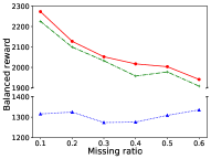
(a) Correlated case on IHDP

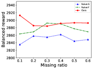
(b) Correlated case on JOBS

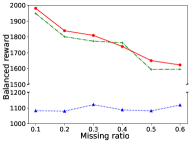
(c) Uncorr. case on IHDP

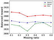
(d) Uncorr. case on JOBS

Figure 1: Comparison of Naive-S, Naive-Y and our method with different missing ratios of $Y$ on IHDP and JOBS, where the metric is the balanced reward.

Policy learning with short-term and long-term reward. We average over 50 independent trials of policy learning with short-term and long-term rewards in IHDP and JOBS, and the results are shown in Table 3. We fix the missing ratio of outcomes $Y$ to be 0.1 and the number of time steps is $T=10$. On one hand, in cases with short-term and long-term metrics, we observe that Naive-S and Naive-Y methods often obtain higher reward/welfare change and lower policy error. However, in cases with balanced capability, our proposed method gives better overall performance. On the other hand, balanced rewards are always higher than short-term or long-term ones in both datasets, which indicates the necessity of balancing short-term and long-term rewards. More results are given in Appendix D.

Effects of varying missing ratios. We study the effects of varying missing ratios for long-term outcome $Y$. As shown in Figures 1(a) and 1(b), our method achieves better performance in almost all scenarios. As the missing ratio increases, both Naive-Y and our method exhibit a declining trend in performance. This decline is expected, as higher missing ratios mean more long-term outcomes are neglected. The performance of Naive-Y is consistently worst.

Effects of varying correlation between $S$ and $Y$. Data generation mechanisms for $Y$ in Eqs. (8) and (9) inherently lead to $S\not\!\perp\!\!\!\perp Y|X$. To compare the distinction between cases with varying correlations, we also generate $Y$ that satisfies $S\perp\!\!\!\perp Y|X$, the data generation details are provided in Appendix E. The results are shown in Figures 1(c) and 1(d). Importantly, comparing Figure 1(a) with Figure 1(c), and Figure 1(b) with Figure 1(d), respectively, we observe that the performance of correlated cases surpasses that in uncorrelated cases. This empirical observation aligns with our findings in Proposition 6.2.

Effects of varying time steps. We further study the impact of varying time steps on long-term outcomes, the associated results are displayed in Figures 2(a) and 2(b), where the missing ratio is set as 0.6. Overall, our method consistently outperforms other baselines across all time steps, even in scenarios with a high missing ratio. More numerical results are available in Appendix D.

Effects of varying costs. According to Eq. (3), we explore the effects of different costs. As depicted in Figures 2(c) and 2(d), in all scenarios with various costs, our method achieves higher balanced rewards compared with Naive-S and Naive-Y, which empirically demonstrates the superiority of taking long-and-short-term rewards into account.

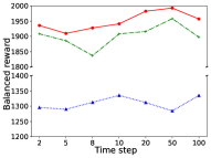
(a) Varying time steps on IHDP

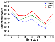
(b) Varying time steps on JOBS

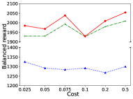
(c) Varying costs on IHDP

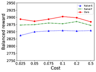
(d) Varying costs on JOBS

Figure 2: Comparison of Naive-S, Naive-Y and ours on IHDP and JOBS, where the metric is the balanced reward.

8 Conclusion

This study delves into an important aspect of interest to empirical researchers and decision-makers in many fields – balancing short-term and long-term rewards. We propose a principled policy learning approach for achieving this goal, which consists of two key steps: estimating the short/long-term rewards for a given policy and learning the optimal policy by taking the estimated short/long-term rewards as the objective functions. We conduct a comprehensive theoretical analysis and perform extensive experiments to demonstrate the effectiveness of the proposed policy learning approach. A limitation of this work is that Assumption 5.1 does not hold in the presence of unmeasured confounders that affects both treatment, short-term and long-term outcomes. Future efforts should focus on extending our method and theory by relaxing identifiability assumptions.

Impact Statements

The paper introduces a novel policy learning approach designed to effectively balance short-term and long-term rewards, overcoming challenges such as confounding bias and missing data in long-term outcomes. This research provides valuable insights and practical implications, particularly in scenarios where optimizing both short-term and long-term outcomes is crucial. Here are some potential applications:

(a) Marketing and customer behavior: marketing professionals can optimize incentive strategies, ensuring they influence customer behavior positively in both the short and long term; (b) Information technology (IT) and user experience: IT companies can design web pages that not only cater to immediate user preferences but also enhance user engagement and satisfaction over an extended period; (c) Healthcare and treatment strategies: medical practitioners can refine drug prescriptions, considering both short-term alleviation and long-term outcomes in chronic diseases like Alzheimer’s and AIDS; (d) Labor market and employment programs: policymakers can enhance the design of job training programs, considering both immediate income impacts and subsequent improvements in employment status; (e) Video recommendation and content engagement: content providers can optimize recommendations, avoiding short-term clickbait strategies that may lead to user churn, ensuring sustained user engagement and revenue growth; etc.

Appendix A Proofs of Proposition 5.3 and Theorem 6.1

Proposition 5.3 (Identifiability of $\mathbb{V}(\pi;y)$). Under Assumptions 5.1-5.2, the long-term reward $\mathbb{V}(\pi;y)$ is identified as

$$\mathbb{V}(\pi;y)={} \mathbb{E}[\pi(X)\tilde{m}_{1}(X,S)+(1-\pi(X))\tilde{m}_{0}(X,S)],$$

where $\tilde{m}_{a}(X,S)=\mathbb{E}[Y|X,S,A=a,R=1]$ for $a=0,1$.

Proof of Proposition 5.3.

The identifiability of $\mathbb{V}(\pi;y)$ can be obtained by noting that

$$\mathbb{V}(\pi;y)={} \mathbb{E}[\pi(X)Y(1)+(1-\pi(X))Y(0)]$$

$$={} \mathbb{E}[\pi(X)\cdot\mathbb{E}(Y(1)|X,S(1))+(1-\pi(X))\cdot\mathbb{E}(Y(0)|X,S(0))]$$

$$={} \mathbb{E}[\pi(X)\cdot\mathbb{E}(Y(1)|X,S(1),A=1)+(1-\pi(X))\cdot\mathbb{E}(Y(0)|X,S(0),A=0)]$$

$$={} \mathbb{E}[\pi(X)\cdot\mathbb{E}(Y(1)|X,S(1),A=1,R=1)]+\mathbb{E}[(1-\pi(X))\cdot\mathbb{E}(Y(0)|X,S(0),A=0,R=1)]$$

$$={} \mathbb{E}[\pi(X)\tilde{m}_{1}(X,S)+(1-\pi(X))\tilde{m}_{0}(X,S)],$$

where the second equality follows by the law of iterated expectations, the third equality follows from Assumption 5.1, and the fourth equality follows from Assumption 5.2. ∎

Theorem 6.1 (Efficiency Bounds of $\mathbb{V}(\pi;s)$ and $\mathbb{V}(\pi;y)$). Under Assumptions 5.1 and 5.2, we have that

(a) the efficient influence function of $\mathbb{V}(\pi;s)$ $\phi_{s}-\mathbb{V}(\pi;s)$, where

$$\phi_{s} ={}\{\pi(X)\mu_{1}(X)+(1-\pi(X))\mu_{0}(X)\}$$

$$+{} \frac{\pi(X)A(S-\mu_{1}(X))}{e(X)}+\frac{(1-\pi(X))(1-A)(S-\mu_{0}(X))}{1-e(X)},$$

the associated semiparametric efficiency bound is $\text{Var}(\phi_{s})$.

(b) the efficient influence functions of $\mathbb{V}(\pi;y)$ is $\phi_{y}-\mathbb{V}(\pi;y)$, where

$$\phi_{y} ={}\{\pi(X)m_{1}(X)+(1-\pi(X))m_{0}(X)\}$$

$$+{} \frac{\pi(X)AR(Y-\tilde{m}_{1}(X,S))}{e(X)r(1,X,S)}+\frac{\pi(X)A(\tilde{m}_{1}(X,S)-m_{1}(X))}{e(X)}$$

$$+{} \frac{(1-\pi(X))(1-A)R(Y-\tilde{m}_{0}(X,S))}{(1-e(X))r(0,X,S)}$$

$$+{} \frac{(1-\pi(X))(1-A)(\tilde{m}_{0}(X,S)-m_{0}(X))}{1-e(X)},$$

the associated semiparametric efficiency bound is $\text{Var}(\phi_{y})$.

Proof of Theorem 6.1.

Let $f(\cdot)$ be the probability density/mass function, $f_{1}(y|x,s)$ and $f_{0}(y|x,s)$ be the density of $Y(1)$ and $Y(0)$ conditional on $(X=x,S(1)=s)$ and $(X=x,S(0)=s)$ respectively, and denote $f_{1}(s|x)$ and $f_{0}(s|x)$ be the density of $S(1)$ and $S(0)$ conditional on $X=x$ respectively. Then the observed data distribution under Assumptions 5.1 and 5.2 is given as

$$p(a,x,s,y,r)$$

$$={} f(a,x,s,y,r=1)^{r}\times f(a,x,s,r=0)^{1-r}$$

$$={} [f(r=1|a,x,s,y)f(a,x,s,y)]^{r}\times[f(r=0|a,x,s)f(a,x,s)]^{1-r}$$

$$={} [r(a,x,s)\cdot\{f(s,y|a=1,x)f(x)e(x)\}^{a}\cdot\{f(s,y|a=0,x)f(x)(1-e(x))\}^{1-a}]^{r}$$

$$\times[(1-r(a,x,s))\cdot\{f(s|x,a=1)f(x)e(x)\}^{a}\cdot\{f(s|x,a=0)f(x)(1-e(x))\}^{1-a}]^{1-r}$$

$$={} f(x)\times[r(a,x,s)\cdot\{f_{1}(y|x,s)f_{1}(s|x)e(x)\}^{a}\cdot\{f_{0}(y|x,s)f_{0}(s|x)(1-e(x))\}^{1-a}]^{r}$$

$$\times[(1-r(a,x,s))\cdot\{f_{1}(s|x)e(x)\}^{a}\cdot\{f_{0}(s|x)(1-e(x))\}^{1-a}]^{1-r}.$$

Under Assumptions 5.1 and 5.2, consider a regular parametric submodel indexed by $\theta$ given as

$$p(a,x,s,y,r;\theta)={} f(x,\theta)\times[r(a,x,s,\theta)\cdot\{f_{1}(y|x,s,\theta)f_{1}(s|x,\theta)e(x,\theta)\}^{a}\cdot\{f_{0}(y|x,s,\theta)f_{0}(s|x,\theta)(1-e(x,\theta))\}^{1-a}]^{r}$$

$$\times[(1-r(a,x,s,\theta))\cdot\{f_{1}(s|x,\theta)e(x,\theta)\}^{a}\cdot\{f_{0}(s|x,\theta)(1-e(x,\theta))\}^{1-a}]^{1-r}.$$

which equals $p(a,x,y,g)$ when $\theta=\theta_{0}$. Also, $f_{a}(y|x,s,\theta_{0})=f_{a}(y|a,x,s,\theta_{0})=f_{a}(y|a,x,s,r=1,\theta_{0})$ for $a=0,1$ by Assumptions 5.1 and 5.2.

Then, the score function for this submodel is given by

$$s(a,x,s,y,r;\theta)=\frac{\partial\log p(a,x,s,y,r;\theta)}{\partial\theta}$$

$$={} s(x,\theta)+ra\cdot\{s_{1}(y|x,s,\theta)+s_{1}(s|x,\theta)\}+r(1-a)\cdot\{s_{0}(y|x,s,\theta)+s_{0}(s|x,\theta)\}$$

$${}+(1-r)a\cdot s_{1}(s|x,\theta)+(1-r)(1-a)\cdot s_{0}(s|x,\theta)$$

$${}+\frac{a-e(x,\theta)}{e(x,\theta)(1-e(x,\theta))}\dot{e}(x,\theta)+\frac{r-r(a,x,s,\theta)}{r(a,x,s,\theta)(1-r(a,x,s,\theta))}\dot{r}(a,x,s,\theta),$$

$$={} s(x,\theta)+ra\cdot s_{1}(y|x,s,\theta)+r(1-a)\cdot s_{0}(y|x,s,\theta)$$

$${}+a\cdot s_{1}(s|x,\theta)+(1-a)\cdot s_{0}(s|x,\theta)$$

$${}+\frac{a-e(x,\theta)}{e(x,\theta)(1-e(x,\theta))}\dot{e}(x,\theta)+\frac{r-r(a,x,s,\theta)}{r(a,x,s,\theta)(1-r(a,x,s,\theta))}\dot{r}(a,x,s,\theta),$$

where

$$s(x,\theta)={} \frac{\partial\log f(x,\theta)}{\partial\theta},$$

$$s_{1}(y|x,s,\theta)={} \frac{\partial\log f_{1}(y|x,s,\theta)}{\partial\theta},$$

$$s_{0}(y|x,s,\theta)={} \frac{\partial\log f_{0}(y|x,s,\theta)}{\partial\theta},$$

$$s_{1}(s|x,\theta)={} \frac{\partial\log f_{1}(s|x,\theta)}{\partial\theta},$$

$$s_{0}(s|x,\theta)={} \frac{\partial\log f_{0}(s|x,\theta)}{\partial\theta},$$

$$\dot{e}(x,\theta)={} \frac{\partial e(x,\theta)}{\partial\theta},$$

$$\dot{r}(a,x,s,\theta)={} \frac{\partial r(a,x,s,\theta)}{\partial\theta}.$$

Thus, the tangent space $\mathcal{T}$ is

$$\mathcal{T}={} \{s(x)+ras_{1}(y|x,s)+r(1-a)s_{0}(y|x,s)+as_{1}(s|x)+(1-a)s_{0}(s|x)$$

$$+(a-e(x))\cdot b(x)+(r-r(a,x,s))\cdot c(x)\},$$

where $s(x)$ satisfies $\mathbb{E}[s(X)]=\int s(x)f(x)dx=0$, $s_{a}(y|a,x,s)$ satisfies $\mathbb{E}[s_{a}(Y|X,S)\big{|}X=x,S=s]=\int s_{a}(y|x,s)f_{a}(y|x,s)dy=0$ for $a=0,1$, $s_{a}(s|x)$ satisfies $\mathbb{E}[s_{a}(S|X)\big{|}X=x]=\int s_{a}(s|x)f_{a}(s|x)ds=0$ for $a=0,1$, and $b(x)$ and $c(x)$ are arbitrary square-intergrable measurable functions of $x$. In addition, $s_{a}(y|a,x,s)=s_{a}(y|a,x,s,r=1)$ according to Assumptions 5.1 and 5.2 (i.e., $f_{a}(y|x,s)=f_{a}(y|a,x,s,r=1)$).

Efficient influence function of short-term reward. Under the above parametric submodel, the short-term reward $\mathbb{V}(\pi;s)$ can be written as

$$\mathbb{V}(\pi, \theta;s)={}\mathbb{E}[\pi(X)S(1)+(1-\pi(X))S(0)]$$

$$={} \int\int\pi(x)sf_{1}(s|x,\theta)f(x,\theta)dsdx+\int\int(1-\pi(x))sf_{0}(s|x,\theta)f(x,\theta)dsdx.$$

The pathwise derivative of $\mathbb{V}(\pi,\theta;s)$ at $\theta=\theta_{0}$ is given as

$$\frac{\partial\mathbb{V}(\pi,\theta;s)}{\partial\theta} \Big{|}_{\theta=\theta_{0}}={}\int\int\pi(x)s\cdot s_{1}(s|x,\theta_{0})f_{1}(s|x,\theta_{0})f(x,\theta_{0})dsdx+\int\int\pi(x)s\cdot f_{1}(s|x,\theta_{0})s(x,\theta_{0})f(x,\theta_{0})dsdx$$

$$+\int\int(1-\pi(x))s\cdot s_{0}(s|x,\theta_{0})f_{0}(s|x,\theta_{0})f(x,\theta_{0})dsdx+\int\int(1-\pi(x))s\cdot f_{0}(s|x,\theta_{0})s(x,\theta_{0})f(x,\theta_{0})dsdx$$

$$={} \mathbb{E}\Big{[}\pi(X)\cdot\mathbb{E}\Big{\{}S(1)\cdot s_{1}(S(1)|X)\Big{|}X\Big{\}}\Big{]}+\mathbb{E}\Big{[}(1-\pi(X))\cdot\mathbb{E}\Big{\{}S(0)\cdot s_{0}(S(0)|X)\Big{|}X\Big{\}}\Big{]}$$

$$+\mathbb{E}\Big{[}s(X)\Big{\{}\pi(X)\mu_{1}(X)+(1-\pi(X))\mu_{0}(X)\Big{\}}\Big{]}.$$

Next, we construct the efficient influence function of $\mathbb{V}(\pi;s)$. Let

$$\tilde{\phi}_{s}=\pi(X)\frac{A(S-\mu_{1}(X))}{e(X)}+(1-\pi(X))\frac{(1-A)(S-\mu_{1}(X))}{1-e(X)}+\{\pi(X)\mu_{1}(X)+(1-\pi(X))\mu_{0}(X)-\mathbb{V}(\pi;s)\}.$$

Pathwise differentiability of $\mathbb{V}(\pi;s)$ can be verified by

$$\frac{\partial\mathbb{V}(\pi,\theta;s)}{\partial\theta}\Big{|}_{\theta=\theta_{0}}=\mathbb{E}[\tilde{\phi}_{s}\cdot s(A,X,S,Y,R;\theta_{0})],$$ (A.1)

which implies that $\tilde{\phi}_{s}$ is an influence function of $\mathbb{V}(\pi;s)$. Now we give a detailed proof of (A.1).

$$\mathbb{E}[\tilde{\phi}_{s}\cdot s(A,X,S,Y,R;\theta_{0})]={} H_{1}+H_{2}+H_{3},$$

where

$$H_{1}={} \mathbb{E}\left[\pi(X)\frac{A(S-\mu_{1}(X))}{e(X)}\cdot s(A,X,S,Y,R;\theta_{0})\right]$$

$$={} \mathbb{E}\Biggl{[}\pi(X)\frac{A(S-\mu_{1}(X))}{e(X)}$$

$${}\times\left\{s(X)+RA\cdot s_{1}(Y|X,S)+A\cdot s_{1}(S|X)+\frac{A-e(X)}{e(X)(1-e(X))}\dot{e}(X)+\frac{R-r(A,X,S)}{r(A,X,S)(1-r(A,X,S))}\dot{r}(A,X,S)\right\}\Biggr{]}$$

$$={} \mathbb{E}\left[\pi(X)\frac{A(S-\mu_{1}(X))}{e(X)}\cdot s_{1}(S|X)\right]$$

$$={} \mathbb{E}\left[\pi(X)\mathbb{E}\left\{(S(1)-\mu_{1}(X))\cdot s_{1}(S(1)|X)\Big{|}X\right\}\right]$$

$$={} \mathbb{E}\left[\pi(X)\mathbb{E}\left\{S(1)\cdot s_{1}(S(1)|X)\Big{|}X\right\}\right]=\text{ the first term of }\frac{\partial\mathbb{V}(\pi,\theta;s)}{\partial\theta}\Big{|}_{\theta=\theta_{0}},$$

and similarly,

$$H_{2}={} \mathbb{E}\left[(1-\pi(X))\frac{(1-A)(S-\mu_{1}(X))}{1-e(X)}\cdot s(A,X,S,Y,R;\theta_{0})\right]$$

$$={} \mathbb{E}\left[(1-\pi(X))\frac{(1-A)(S-\mu_{1}(X))}{1-e(X)}\cdot s_{0}(S|X)\right]$$

$$={} \mathbb{E}\left[(1-\pi(X))\mathbb{E}\left\{S(0)\cdot s_{0}(S(0)|X)\Big{|}X\right\}\right]=\text{ the second term of }\frac{\partial\mathbb{V}(\pi,\theta;s)}{\partial\theta}\Big{|}_{\theta=\theta_{0}},$$

$$H_{3}={} \mathbb{E}\left[\{\pi(X)\mu_{1}(X)+(1-\pi(X))\mu_{0}(X)-\mathbb{V}(\pi;s)\}\cdot s(A,X,S,Y,R;\theta_{0})\right]$$

$$={} \mathbb{E}\left[\{\pi(X)\mu_{1}(X)+(1-\pi(X))\mu_{0}(X)-\mathbb{V}(\pi;s)\}\cdot s(X)\right]$$

$$={} \mathbb{E}\Big{[}s(X)\Big{\{}\pi(X)\mu_{1}(X)+(1-\pi(X))\mu_{0}(X)\Big{\}}\Big{]}=\text{ the third term of }\frac{\partial\mathbb{V}(\pi,\theta;s)}{\partial\theta}\Big{|}_{\theta=\theta_{0}},$$

Thus, equation (A.1) holds. In addition, let $s(X)=\{\pi(X)\mu_{1}(X)+(1-\pi(X))\mu_{0}(X)-\mathbb{V}(\pi;s)\}$, $s_{1}(Y|X)=\pi(X)\frac{(S-\mu_{1}(X))}{e(X)}$, $s_{0}(S|X)=(1-\pi(X))\frac{(S-\mu_{1}(X))}{1-e(X)}$, then $\tilde{\phi}_{s}$ can be written as

$$\tilde{\phi}_{s}=s(X)+As_{1}(S|X)+(1-A)s_{0}(S|X).$$

Clearly, we have that $\int s_{a}(s|x)f_{a}(s|x)ds=0$ and $\int s(x)f(x)dx=0$, which implies that $\tilde{\phi}_{s}\in\mathcal{T}$, and thus $\tilde{\phi}_{s}$ is the efficient influence function of $\mathbb{V}(\pi;s)$.

Efficient influence function of long-term reward. Under the above parametric submodel, the long-term reward $\mathbb{V}(\pi;y)$ can be written as

$$\mathbb{V}(\pi, \theta;y)={}\mathbb{E}[\pi(X)Y(1)+(1-\pi(X))Y(0)]$$

$$={} \mathbb{E}\Big{[}\pi(X)\mathbb{E}\{Y(1)|S(1),X\}+(1-\pi(X))\mathbb{E}\{Y(0)|S(0),X\}\Big{]}$$

$$={} \int\int\int\pi(x)yf_{1}(y|x,s,\theta)f_{1}(s|x,\theta)f(x,\theta)dydsdx+\int\int\int(1-\pi(x))yf_{0}(y|x,s,\theta)f_{0}(s|x,\theta)f(x,\theta)dydsdx.$$

The pathwise derivative of $\mathbb{V}(\pi,\theta;y)$ at $\theta=\theta_{0}$ is given as

$$\frac{\partial\mathbb{V}(\pi,\theta;y)}{\partial\theta} \Big{|}_{\theta=\theta_{0}}={}\int\int\int\pi(x)ys_{1}(y|x,s,\theta_{0})f_{1}(y|x,s,\theta_{0})\cdot f_{1}(s|x,\theta_{0})f(x,\theta_{0})dydsdx$$

$$+\int\int\int\pi(x)yf_{1}(y|x,s,\theta_{0})\cdot\Big{\{}s_{1}(s|x,\theta_{0})f_{1}(s|x,\theta_{0})f(x,\theta_{0})+f_{1}(s|x,\theta_{0})s(x,\theta_{0})f(x,\theta_{0})\Big{\}}dydsdx$$

$$+\int\int\int(1-\pi(x))ys_{0}(y|x,s,\theta_{0})f_{0}(y|x,s,\theta_{0})\cdot f_{0}(s|x,\theta_{0})f(x,\theta_{0})dydsdx$$

$$+\int\int\int(1-\pi(x))yf_{0}(y|x,s,\theta_{0})\cdot\Big{\{}s_{0}(s|x,\theta_{0})f_{0}(s|x,\theta_{0})f(x,\theta_{0})+f_{0}(s|x,\theta_{0})s(x,\theta_{0})f(x,\theta_{0})\Big{\}}dydsdx$$

$$={} \mathbb{E}\Big{[}\pi(X)\cdot\mathbb{E}\Big{\{}Y(1)\cdot s_{1}(Y(1)|X,S)\Big{|}X,S\Big{\}}\Big{]}+\mathbb{E}\Big{[}(1-\pi(X))\cdot\mathbb{E}\Big{\{}Y(0)\cdot s_{0}(Y(0)|X,S)\Big{|}X,S\Big{\}}\Big{]}$$

$$+\mathbb{E}\Big{[}\pi(X)\cdot\mathbb{E}\Big{\{}\tilde{m}_{1}(X,S)\cdot s_{1}(S(1)|X)\Big{|}X\Big{\}}\Big{]}+\mathbb{E}\Big{[}(1-\pi(X))\cdot\mathbb{E}\Big{\{}\tilde{m}_{0}(X,S)\cdot s_{0}(S(0)|X)\Big{|}X\Big{\}}\Big{]}$$

$$+\mathbb{E}\Big{[}s(X)\Big{\{}\pi(X)\tilde{m}_{1}(X,S)+(1-\pi(X))\tilde{m}_{0}(X,S)\Big{\}}\Big{]}$$

$$={} \mathbb{E}\Big{[}\pi(X)\cdot\mathbb{E}\Big{\{}Y(1)\cdot s_{1}(Y(1)|X,S)\Big{|}X,S\Big{\}}\Big{]}+\mathbb{E}\Big{[}(1-\pi(X))\cdot\mathbb{E}\Big{\{}Y(0)\cdot s_{0}(Y(0)|X,S)\Big{|}X,S\Big{\}}\Big{]}$$

$$+\mathbb{E}\Big{[}\pi(X)\cdot\mathbb{E}\Big{\{}\tilde{m}_{1}(X,S)\cdot s_{1}(S(1)|X)\Big{|}X\Big{\}}\Big{]}+\mathbb{E}\Big{[}(1-\pi(X))\cdot\mathbb{E}\Big{\{}\tilde{m}_{0}(X,S)\cdot s_{0}(S(0)|X)\Big{|}X\Big{\}}\Big{]}$$

$$+\mathbb{E}\Big{[}s(X)\Big{\{}\pi(X)m_{1}(X)+(1-\pi(X))m_{0}(X)\Big{\}}\Big{]},$$

where the last equation follows from $\mathbb{E}[\tilde{m}_{a}(X,S)|X]=m_{a}(X)$ for $a=0,1$.

Next, we construct the efficient influence function of $\mathbb{V}(\pi;y)$. Let

$$\tilde{\phi}_{y}={} \pi(X)\frac{AR(Y-\tilde{m}_{1}(X,S))}{e(X)r(1,X,S)}+(1-\pi(X))\frac{(1-A)R(Y-\tilde{m}_{0}(X,S))}{(1-e(X))r(0,X,S)}$$

$$+\pi(X)\frac{A(\tilde{m}_{1}(X,S)-m_{1}(X))}{e(X)}+(1-\pi(X))\frac{(1-A)(\tilde{m}_{0}(X,S)-m_{0}(X))}{1-e(X)}$$

$$+\{\pi(X)m_{1}(X)+(1-\pi(X))m_{0}(X)-\mathbb{V}(\pi;y)\}.$$

Pathwise differentiability of $\mathbb{V}(\pi;y)$ can be verified by

$$\frac{\partial\mathbb{V}(\pi,\theta;y)}{\partial\theta}\Big{|}_{\theta=\theta_{0}}=\mathbb{E}[\tilde{\phi}_{y}\cdot s(A,X,S,Y,R;\theta_{0})],$$ (A.2)

which implies that $\tilde{\phi}_{y}$ is an influence function of $\mathbb{V}(\pi;y)$. Now we give a detailed proof of (A.2). The right side of (A.2) can be decomposed as

$$\mathbb{E}[\tilde{\phi}_{y}\cdot s(A,X,S,Y,R;\theta_{0})]=H_{4}+H_{5}+H_{6}+H_{7}+H_{8},$$

where

$$H_{4}={} \mathbb{E}\left[\pi(X)\frac{AR(Y-\tilde{m}_{1}(X,S))}{e(X)r(1,X,S)}\cdot s(A,X,S,Y,R;\theta_{0})\right]$$

$$={} \mathbb{E}\Biggl{[}\pi(X)\frac{AR(Y-\tilde{m}_{1}(X,S))}{e(X)r(1,X,S)}\cdot s_{1}(Y|X,S)\Biggr{]}$$

$$={} \mathbb{E}\left[\pi(X)\mathbb{E}\left\{(Y(1)-\tilde{m}_{1}(X,S))\cdot s_{1}(Y(1)|X,S)\Big{|}X,S\right\}\right]$$

$$={} \mathbb{E}\left[\pi(X)\mathbb{E}\left\{Y(1)\cdot s_{1}(Y(1)|X,S)\Big{|}X,S\right\}\right]=\text{ the first term of }\frac{\partial\mathbb{V}(\pi,\theta;y)}{\partial\theta}\Big{|}_{\theta=\theta_{0}},$$

$$H_{5}={} \mathbb{E}\left[(1-\pi(X))\frac{(1-A)R(Y-\tilde{m}_{0}(X,S))}{(1-e(X))r(0,X,S)}\cdot s(A,X,S,Y,R;\theta_{0})\right]$$

$$={} \mathbb{E}\Biggl{[}(1-\pi(X))\frac{(1-A)R(Y-\tilde{m}_{0}(X,S))}{(1-e(X))r(0,X,S)}\cdot s_{0}(Y|X,S)\Biggr{]}$$

$$={} \mathbb{E}\left[\pi(X)\mathbb{E}\left\{Y(0)\cdot s_{1}(Y(0)|X,S)\Big{|}X,S\right\}\right]=\text{ the second term of }\frac{\partial\mathbb{V}(\pi,\theta;y)}{\partial\theta}\Big{|}_{\theta=\theta_{0}},$$

$$H_{6}={} \mathbb{E}\left[\pi(X)\frac{A(\tilde{m}_{1}(X,S)-m_{1}(X))}{e(X)}\cdot s(A,X,S,Y,R;\theta_{0})\right]$$

$$={} \mathbb{E}\left[\pi(X)\frac{A(\tilde{m}_{1}(X,S)-m_{1}(X))}{e(X)}\cdot As_{1}(S|X)\right]$$

$$={} \mathbb{E}\left[\pi(X)\cdot\mathbb{E}\left\{(\tilde{m}_{1}(X,S)-m_{1}(X))\cdot s_{1}(S(1)|X)\Big{|}X\right\}\right]$$

$$={} \mathbb{E}\left[\pi(X)\cdot\mathbb{E}\left\{\tilde{m}_{1}(X,S)\cdot s_{1}(S(1)|X)\Big{|}X\right\}\right]=\text{ the third term of }\frac{\partial\mathbb{V}(\pi,\theta;y)}{\partial\theta}\Big{|}_{\theta=\theta_{0}},$$

$$H_{7}={} \mathbb{E}\left[(1-\pi(X))\frac{(1-A)(\tilde{m}_{0}(X,S)-m_{0}(X))}{1-e(X)}\cdot s(A,X,S,Y,R;\theta_{0})\right]$$

$$={} \mathbb{E}\Biggl{[}(1-\pi(X))\frac{(1-A)(\tilde{m}_{0}(X,S)-m_{0}(X))}{1-e(X)}\cdot(1-A)s_{0}(S|X)\Biggr{]}$$

$$={} \mathbb{E}\Big{[}(1-\pi(X))\cdot\mathbb{E}\Big{\{}\tilde{m}_{0}(X,S)\cdot s_{0}(S(0)|X)\Big{|}X\Big{\}}\Big{]}=\text{ the fourth term of }\frac{\partial\mathbb{V}(\pi,\theta;y)}{\partial\theta}\Big{|}_{\theta=\theta_{0}},$$

and

$$H_{8}={} \mathbb{E}\left[\{\pi(X)m_{1}(X)+(1-\pi(X))m_{0}(X)-\mathbb{V}(\pi;y)\}\cdot s(A,X,S,Y,R;\theta_{0})\right]$$

$$={} \mathbb{E}\left[\{\pi(X)m_{1}(X)+(1-\pi(X))m_{0}(X)-\mathbb{V}(\pi;y)\}\cdot s(X)\right]$$

$$={} \mathbb{E}\Big{[}s(X)\Big{\{}\pi(X)m_{1}(X)+(1-\pi(X))m_{0}(X)\Big{\}}\Big{]}=\text{ the last term of }\frac{\partial\mathbb{V}(\pi,\theta;y)}{\partial\theta}\Big{|}_{\theta=\theta_{0}}.$$

Thus, equation (A.2) holds. In addition, it can be shown that $\tilde{\phi}_{y}\in\mathcal{T}$, and thus $\tilde{\phi}_{y}$ is the efficient influence function of $\mathbb{V}(\pi;y)$.

∎

Appendix B Proofs of Propositions 6.2-6.3, Theorem 6.4, and Proposition 6.5

Proposition 6.2. Under the conditions in Theorem 6.1, if $S$ is associated with $Y$ given $X$, then the semiparametric efficiency bound of $\mathbb{V}(\pi;y)$ is lower compared to the case where $S\perp\!\!\!\perp Y|X$, and the magnitude of this difference is

$$\mathbb{E}\left[\pi^{2}(X)\frac{(1-r(1,X,S))\cdot(\tilde{m}_{1}(X,S)-m_{1}(X))^{2}}{e(X)r(1,X,S)}+(1-\pi(X))^{2}\frac{(1-r(0,X,S))\cdot(\tilde{m}_{0}(X,S)-m_{0}(X))^{2}}{(1-e(X))r(0,X,S)}\right].$$

Proof of Proposition 6.2.

If $S$ is associated with $Y$ given $X$, then the efficient influence function for $\mathbb{V}(\pi;y)$ is

$$\tilde{\phi}_{y}={} \pi(X)\frac{AR(Y-\tilde{m}_{1}(X,S))}{e(X)r(1,X,S)}+(1-\pi(X))\frac{(1-A)R(Y-\tilde{m}_{0}(X,S))}{(1-e(X))r(0,X,S)}$$

$$+\pi(X)\frac{A(\tilde{m}_{1}(X,S)-m_{1}(X))}{e(X)}+(1-\pi(X))\frac{(1-A)(\tilde{m}_{0}(X,S)-m_{0}(X))}{1-e(X)}$$

$$+\{\pi(X)m_{1}(X)+(1-\pi(X))m_{0}(X)-\mathbb{V}(\pi;y)\},$$

and the semiparametric efficiency bound is

$$\text{Var}(\tilde{\phi}_{y})={} \mathbb{E}[\{\pi(X)m_{1}(X)+(1-\pi(X))m_{0}(X)-\mathbb{V}(\pi;y)\}^{2}]+\mathbb{E}\left[\pi^{2}(X)\frac{AR(Y-\tilde{m}_{1}(X,S))^{2}}{e^{2}(X)r^{2}(1,X,S)}\right]$$

$$+\mathbb{E}\left[(1-\pi(X))^{2}\frac{(1-A)R(Y-\tilde{m}_{0}(X,S))^{2}}{(1-e(X))^{2}r^{2}(0,X,S)}\right]+\mathbb{E}\left[\pi^{2}(X)\frac{A(\tilde{m}_{1}(X,S)-m_{1}(X))^{2}}{e^{2}(X)}\right]$$

$$+\mathbb{E}\left[(1-\pi(X))^{2}\frac{(1-A)(\tilde{m}_{0}(X,S)-m_{0}(X))^{2}}{(1-e(X))^{2}}\right]$$

$$={} \mathbb{E}[\{\pi(X)m_{1}(X)+(1-\pi(X))m_{0}(X)-\mathbb{V}(\pi;y)\}^{2}]+\mathbb{E}\left[\pi^{2}(X)\frac{\mathbb{E}\{(Y-\tilde{m}_{1}(X,S))^{2}|X,S,A=1,R=1\}}{e(X)r(1,X,S)}\right]$$

$$+\mathbb{E}\left[(1-\pi(X))^{2}\frac{\mathbb{E}\{(Y-\tilde{m}_{0}(X,S))^{2}|X,S,A=0,R=1\}}{(1-e(X))r(0,X,S)}\right]+\mathbb{E}\left[\pi^{2}(X)\frac{\mathbb{E}\{(\tilde{m}_{1}(X,S)-m_{1}(X))^{2}|X\}}{e(X)}\right]$$

$$+\mathbb{E}\left[(1-\pi(X))^{2}\frac{\mathbb{E}\{(\tilde{m}_{0}(X,S)-m_{0}(X))^{2}|X\}}{(1-e(X))}\right]$$

$$={} \mathbb{E}[\{\pi(X)m_{1}(X)+(1-\pi(X))m_{0}(X)-\mathbb{V}(\pi;y)\}^{2}]+\mathbb{E}\left[\pi^{2}(X)\frac{(Y-\tilde{m}_{1}(X,S))^{2}}{e(X)r(1,X,S)}\right]$$

$$+\mathbb{E}\left[(1-\pi(X))^{2}\frac{(Y-\tilde{m}_{0}(X,S))^{2}}{(1-e(X))r(0,X,S)}\right]+\mathbb{E}\left[\pi^{2}(X)\frac{(\tilde{m}_{1}(X,S)-m_{1}(X))^{2}}{e(X)}\right]$$

$$+\mathbb{E}\left[(1-\pi(X))^{2}\frac{(\tilde{m}_{0}(X,S)-m_{0}(X))^{2}}{(1-e(X))}\right],$$

where the first equality holds because the covariance terms are 0, the second equality follows by law of iterated expectations, and the third equality follows by Assumptions 5.1-5.2. Likewise, if $S\perp\!\!\!\perp Y|X$, then $\tilde{m}_{a}(X,S)=m_{a}(X)$, the efficient influence function for $\mathbb{V}(\pi;y)$ simplifies to

$$\bar{\phi}_{y}={} \pi(X)\frac{AR(Y-m_{1}(X))}{e(X)r(1,X,S)}+(1-\pi(X))\frac{(1-A)R(Y-m_{0}(X))}{(1-e(X))r(0,X,S)}$$

$$+\{\pi(X)m_{1}(X)+(1-\pi(X))m_{0}(X)-\mathbb{V}(\pi;y)\},$$

and the semiparametric efficiency bound is

$$\text{Var}(\bar{\phi}_{y})={} \mathbb{E}[\{\pi(X)m_{1}(X)+(1-\pi(X))m_{0}(X)-\mathbb{V}(\pi;y)\}^{2}]+\mathbb{E}\left[\pi^{2}(X)\frac{AR(Y-m_{1}(X))^{2}}{e^{2}(X)r^{2}(1,X,S)}\right]$$

$$+\mathbb{E}\left[(1-\pi(X))^{2}\frac{(1-A)R(Y-m_{0}(X))^{2}}{(1-e(X))^{2}r^{2}(0,X,S)}\right]$$

$$={} \mathbb{E}[\{\pi(X)m_{1}(X)+(1-\pi(X))m_{0}(X)-\mathbb{V}(\pi;y)\}^{2}]+\mathbb{E}\left[\pi^{2}(X)\frac{(Y-m_{1}(X))^{2}}{e(X)r(1,X,S)}\right]$$

$$+\mathbb{E}\left[(1-\pi(X))^{2}\frac{(Y-m_{0}(X))^{2}}{(1-e(X))r(0,X,S)}\right].$$

Thus, the magnitude of their difference is

$$\text{Var}(\bar{\phi}_{y}) -\text{Var}(\tilde{\phi}_{y})={}\mathbb{E}\left[\pi^{2}(X)\frac{(Y-m_{1}(X))^{2}}{e(X)r(1,X,S)}+(1-\pi(X))^{2}\frac{(Y-m_{0}(X))^{2}}{(1-e(X))r(0,X,S)}\right]$$

$$-\mathbb{E}\left[\pi^{2}(X)\frac{(Y-\tilde{m}_{1}(X,S))^{2}}{e(X)r(1,X,S)}\right]-\mathbb{E}\left[(1-\pi(X))^{2}\frac{(Y-\tilde{m}_{0}(X,S))^{2}}{(1-e(X))r(0,X,S)}\right]$$

$$-\mathbb{E}\left[\pi^{2}(X)\frac{(\tilde{m}_{1}(X,S)-m_{1}(X))^{2}}{e(X)}\right]-\mathbb{E}\left[(1-\pi(X))^{2}\frac{(\tilde{m}_{0}(X,S)-m_{0}(X))^{2}}{(1-e(X))}\right]$$

$$={} \mathbb{E}\left[\pi^{2}(X)\frac{(Y-\tilde{m}_{1}(X,S)+\tilde{m}_{1}(X,S)-m_{1}(X))^{2}}{e(X)r(1,X,S)}+(1-\pi(X))^{2}\frac{(Y-\tilde{m}_{0}(X,S)+\tilde{m}_{1}(X,S)-m_{0}(X))^{2}}{(1-e(X))r(0,X,S)}\right]$$

$$-\mathbb{E}\left[\pi^{2}(X)\frac{(Y-\tilde{m}_{1}(X,S))^{2}}{e(X)r(1,X,S)}\right]-\mathbb{E}\left[(1-\pi(X))^{2}\frac{(Y-\tilde{m}_{0}(X,S))^{2}}{(1-e(X))r(0,X,S)}\right]$$

$$-\mathbb{E}\left[\pi^{2}(X)\frac{(\tilde{m}_{1}(X,S)-m_{1}(X))^{2}}{e(X)}\right]-\mathbb{E}\left[(1-\pi(X))^{2}\frac{(\tilde{m}_{0}(X,S)-m_{0}(X))^{2}}{(1-e(X))}\right]$$

$$={} \mathbb{E}\left[\pi^{2}(X)\frac{(\tilde{m}_{1}(X,S)-m_{1}(X))^{2}}{e(X)r(1,X,S)}+(1-\pi(X))^{2}\frac{(\tilde{m}_{0}(X,S)-m_{0}(X))^{2}}{(1-e(X))r(0,X,S)}\right]$$

$$-\mathbb{E}\left[\pi^{2}(X)\frac{(\tilde{m}_{1}(X,S)-m_{1}(X))^{2}}{e(X)}\right]-\mathbb{E}\left[(1-\pi(X))^{2}\frac{(\tilde{m}_{0}(X,S)-m_{0}(X))^{2}}{(1-e(X))}\right]$$

$$={} \mathbb{E}\left[\pi^{2}(X)\frac{(1-r(1,X,S))\cdot(\tilde{m}_{1}(X,S)-m_{1}(X))^{2}}{e(X)r(1,X,S)}+(1-\pi(X))^{2}\frac{(1-r(0,X,S))\cdot(\tilde{m}_{0}(X,S)-m_{0}(X))^{2}}{(1-e(X))r(0,X,S)}\right],$$

which leads to the conclusion by noting that $\pi(X)^{2}=\pi(X)$ and $(1-\pi(X))^{2}=1-\pi(X)$. ∎

Proposition 6.3 (Unbiasedness). We have that

(a) (Double Robustness). $\hat{\mathbb{V}}(\pi;s)$ is an unbiased estimator of $\mathbb{V}(\pi;s)$ if one of the following conditions is satisfied:

• $\hat{e}(x)=e(x)$, i.e., $\hat{e}(x)$ estimates $e(x)$ accurately;

• $\hat{\mu}_{a}(x)=\mu(x)$ i.e., $\mu_{a}(x)$ estimates $\mu_{a}(x)$ accurately.

(b) (Quadruple Robustness). $\hat{\mathbb{V}}(\pi;y)$ is an unbiased estimator of $\mathbb{V}(\pi;y)$ if one of the following conditions is satisfied:

• $\hat{e}(x)=e(x)$ and $\hat{\tilde{m}}_{a}(x,s)=\tilde{m}_{a}(x,s)$;

• $\hat{e}(x)=e(x)$ and $\hat{r}(a,x,s)=r(a,x,s)$;

• $\hat{m}_{a}(x)=m_{a}(x)$ and $\hat{\tilde{m}}_{a}(x,s)=\tilde{m}_{a}(x,s)$;

• $\hat{m}_{a}(x)=m_{a}(x)$ and $\hat{r}(a,x,s)=r(a,x,s)$.

Proof of Proposition 6.3.

Recall that $Z=(X,A,S,Y)$,

$$\phi_{s}(Z;e,\mu_{0},\mu_{1}) ={}\{\pi(X)\mu_{1}(X)+(1-\pi(X))\mu_{0}(X)\}+\frac{\pi(X)A(S-\mu_{1}(X))}{e(X)}+\frac{(1-\pi(X))(1-A)(S-\mu_{0}(X))}{1-e(X)},$$

$$\phi_{y}(Z;e,r, m_{0},m_{1},\tilde{m}_{0},\tilde{m}_{1})={}\{\pi(X)m_{1}(X)+(1-\pi(X))m_{0}(X)\}$$

$$+{} \frac{\pi(X)AR(Y-\tilde{m}_{1}(X,S))}{e(X)r(1,X,S)}+\frac{\pi(X)A(\tilde{m}_{1}(X,S)-m_{1}(X))}{e(X)}$$

$$+{} \frac{(1-\pi(X))(1-A)R(Y-\tilde{m}_{0}(X,S))}{(1-e(X))r(0,X,S)}+\frac{(1-\pi(X))(1-A)(\tilde{m}_{0}(X,S)-m_{0}(X))}{1-e(X)},$$

and

$$\hat{\mathbb{V}}(\pi;s)={} \frac{1}{n}\sum_{i=1}^{n}\phi_{s}(Z_{i};\hat{e},\hat{\mu}_{0},\hat{\mu}_{1}),$$

$$\hat{\mathbb{V}}(\pi;y)={} \frac{1}{n}\sum_{i=1}^{n}\phi_{y}(Z_{i};\hat{e},\hat{r},\hat{m}_{0},\hat{m}_{1},\hat{\tilde{m}}_{0},\hat{\tilde{m}}_{1}).$$

Next, we prove (a) and (b) separately.

Proof of (a). Due to the sample splitting, $\hat{e}(X_{i})$ and $\mu_{a}(X_{i})$ can be seen as an function of $X_{i}$ when taking expectation of $\mathbb{E}[\hat{\mathbb{V}}(\pi;s)]$. Thus,

$$\mathbb{E}[ \hat{\mathbb{V}}(\pi;s)]={}\mathbb{E}[\phi_{s}(Z;\hat{e},\hat{\mu}_{0},\hat{\mu}_{1})]$$

$$={} \mathbb{E}\left[\{\pi(X)\hat{\mu}_{1}(X)+(1-\pi(X))\hat{\mu}_{0}(X)\}+\frac{\pi(X)A(S-\hat{\mu}_{1}(X))}{\hat{e}(X)}+\frac{(1-\pi(X))(1-A)(S-\hat{\mu}_{0}(X))}{1-\hat{e}(X)}\right]$$

$$={} \mathbb{E}\left[\{\pi(X)\hat{\mu}_{1}(X)+(1-\pi(X))\hat{\mu}_{0}(X)\}+\frac{\pi(X)A(S(1)-\hat{\mu}_{1}(X))}{\hat{e}(X)}+\frac{(1-\pi(X))(1-A)(S(0)-\hat{\mu}_{0}(X))}{1-\hat{e}(X)}\right]$$

$$={} \mathbb{E}\left[\{\pi(X)\hat{\mu}_{1}(X)+(1-\pi(X))\hat{\mu}_{0}(X)\}\right]+\mathbb{E}\left[\frac{\pi(X)e(X)(\mu_{1}(X)-\hat{\mu}_{1}(X))}{\hat{e}(X)}+\frac{(1-\pi(X))(1-e(X))(\mu_{0}(X)-\hat{\mu}_{0}(X))}{1-\hat{e}(X)}\right],$$

where the last equality follows by the law of iterated expectations and Assumption 5.1.

If $\hat{e}(X)=e(X)$, $\mathbb{E}[\hat{\mathbb{V}}(\pi;s)]$ reduces to

$$\mathbb{E}\left[\{\pi(X)\hat{\mu}_{1}(X)+(1-\pi(X))\hat{\mu}_{0}(X)\}\right]+\mathbb{E}\left[\pi(X)(\mu_{1}(X)-\hat{\mu}_{1}(X))+(1-\pi(X))(\mu_{0}(X)-\hat{\mu}_{0}(X))\right]$$

$$={} \mathbb{E}\left[\pi(X)\mu_{1}(X)+(1-\pi(X))\mu_{0}(X)\right]$$

$$={} \mathbb{V}(\pi;s).\qquad\text{By equation (\ref{eq4})}$$

This proves the conclusion (a)(i).

If $\hat{\mu}_{a}(X)=\mu_{a}(X)$ for $a=0,1$, $\mathbb{E}[\hat{\mathbb{V}}(\pi;s)]$ reduces to

$$\mathbb{E}\left[\{\pi(X)\hat{\mu}_{1}(X)+(1-\pi(X))\hat{\mu}_{0}(X)\}\right]+0$$

$$={} \mathbb{E}\left[\pi(X)\mu_{1}(X)+(1-\pi(X))\mu_{0}(X)\right]$$

$$={} \mathbb{V}(\pi;s).$$

This proves the conclusion (a)(ii).

Proof of (b). Similar to the proof of (a), we first calculate the expectation of $\hat{\mathbb{V}}(\pi;y)$.

$$\mathbb{E}[\hat{\mathbb{V}}(\pi;y)]$$

$$={} \mathbb{E}[\phi_{y}(Z;\hat{e},\hat{r},\hat{m}_{0},\hat{m}_{1},\hat{\tilde{m}}_{0},\hat{\tilde{m}}_{1}]$$

$$={} \mathbb{E}\left[\pi(X)\hat{m}_{1}(X)+(1-\pi(X))\hat{m}_{0}(X)\right]$$

$$+{} \mathbb{E}\left[\frac{\pi(X)AR(Y-\hat{\tilde{m}}_{1}(X,S))}{\hat{e}(X)\hat{r}(1,X,S)}+\frac{\pi(X)A(\hat{\tilde{m}}_{1}(X,S)-\hat{m}_{1}(X))}{\hat{e}(X)}\right]$$

$$+{} \mathbb{E}\left[\frac{(1-\pi(X))(1-A)R(Y-\hat{\tilde{m}}_{0}(X,S))}{(1-\hat{e}(X))\hat{r}(0,X,S)}+\frac{(1-\pi(X))(1-A)(\hat{\tilde{m}}_{0}(X,S)-\hat{m}_{0}(X))}{1-\hat{e}(X)}\right]$$

$$={} \mathbb{E}\left[\pi(X)\hat{m}_{1}(X)+(1-\pi(X))\hat{m}_{0}(X)\right]$$

$$+{} \mathbb{E}\left[\frac{\pi(X)\cdot\mathbb{E}[AR(Y-\hat{\tilde{m}}_{1}(X,S))\mid X,S]}{\hat{e}(X)\hat{r}(1,X,S)}+\frac{\pi(X)e(X)(\hat{\tilde{m}}_{1}(X,S)-\hat{m}_{1}(X))}{\hat{e}(X)}\right]$$

$$+{} \mathbb{E}\left[\frac{(1-\pi(X))\cdot\mathbb{E}[(1-A)R(Y-\hat{\tilde{m}}_{0}(X,S))\mid X,S]}{(1-\hat{e}(X))\hat{r}(0,X,S)}+\frac{(1-\pi(X))(1-e(X))(\hat{\tilde{m}}_{0}(X,S)-\hat{m}_{0}(X))}{1-\hat{e}(X)}\right]$$

$$={} \mathbb{E}\left[\pi(X)\hat{m}_{1}(X)+(1-\pi(X))\hat{m}_{0}(X)\right]$$

$$+{} \mathbb{E}\left[\frac{\pi(X)\cdot\mathbb{E}[(Y-\hat{\tilde{m}}_{1}(X,S))\mid X,S,A=1,R=1]\cdot\mathbb{P}(A=1,R=1|X,S)}{\hat{e}(X)\hat{r}(1,X,S)}+\frac{\pi(X)e(X)(\hat{\tilde{m}}_{1}(X,S)-\hat{m}_{1}(X))}{\hat{e}(X)}\right]$$

$$+{} \mathbb{E}\left[\frac{(1-\pi(X))\cdot\mathbb{E}[((Y-\hat{\tilde{m}}_{0}(X,S))\mid X,S,A=0,R=1]\cdot\mathbb{P}(A=0,R=1|X,S)}{(1-\hat{e}(X))\hat{r}(0,X,S)}\right]$$

$$+{} \mathbb{E}\left[\frac{(1-\pi(X))(1-e(X))(\hat{\tilde{m}}_{0}(X,S)-\hat{m}_{0}(X))}{1-\hat{e}(X)}\right]$$

$$={} \mathbb{E}\left[\pi(X)\hat{m}_{1}(X)+(1-\pi(X))\hat{m}_{0}(X)\right]$$

$$+{} \mathbb{E}\left[\frac{\pi(X)\cdot\{\tilde{m}_{1}(X,S)-\hat{\tilde{m}}_{1}(X,S)\}\cdot e(X)r(1,X,S)}{\hat{e}(X)\hat{r}(1,X,S)}+\frac{\pi(X)e(X)(\hat{\tilde{m}}_{1}(X,S)-\hat{m}_{1}(X))}{\hat{e}(X)}\right]$$

$$+{} \mathbb{E}\left[\frac{(1-\pi(X))\cdot\{\tilde{m}_{0}(X,S)-\hat{\tilde{m}}_{0}(X,S)\}\cdot(1-e(X))r(0,X,S)}{(1-\hat{e}(X))\hat{r}(0,X,S)}+\frac{(1-\pi(X))(1-e(X))(\hat{\tilde{m}}_{0}(X,S)-\hat{m}_{0}(X))}{1-\hat{e}(X)}\right].$$

If $\hat{e}(X)=e(X)$ and $\hat{\tilde{m}}_{a}(X,S)=\tilde{m}_{a}(X,S)$, $\mathbb{E}[\hat{\mathbb{V}}(\pi;y)]$ reduces to

$$\mathbb{E}\left[\pi(X)\hat{m}_{1}(X)+(1-\pi(X))\hat{m}_{0}(X)\right]$$

$$+{} \mathbb{E}\left[\pi(X)({\tilde{m}}_{1}(X,S)-\hat{m}_{1}(X))+(1-\pi(X))({\tilde{m}}_{0}(X,S)-\hat{m}_{0}(X))\right]$$

$$={} \mathbb{E}[\pi(X)\tilde{m}_{1}(X,S)+(1-\pi(X))\tilde{m}_{0}(X,S)]$$

$$={} \mathbb{V}(\pi;y).\qquad\text{by Proposition \ref{prop5-3}}$$

This proves (b)(i).

If $\hat{e}(X)=e(X)$ and $\hat{r}(a,X,S)=r(a,X,S)$, $\mathbb{E}[\hat{\mathbb{V}}(\pi;y)]$ reduces to

$$\mathbb{E}\left[\pi(X)\hat{m}_{1}(X)+(1-\pi(X))\hat{m}_{0}(X)\right]$$

$$+{} \mathbb{E}\left[\pi(X)\cdot\{\tilde{m}_{1}(X,S)-\hat{\tilde{m}}_{1}(X,S)\}+\pi(X)(\hat{\tilde{m}}_{1}(X,S)-\hat{m}_{1}(X))\right]$$

$$+{} \mathbb{E}\left[(1-\pi(X))\cdot\{\tilde{m}_{0}(X,S)-\hat{\tilde{m}}_{0}(X,S)\}+(1-\pi(X))(\hat{\tilde{m}}_{0}(X,S)-\hat{m}_{0}(X))\right]$$

$$={} \mathbb{E}[\pi(X)\tilde{m}_{1}(X,S)+(1-\pi(X))\tilde{m}_{0}(X,S)]$$

$$={} \mathbb{V}(\pi;y).$$

This proves (b)(ii).

If $\hat{m}_{a}(X)=m_{a}(X)$ and $\hat{\tilde{m}}_{a}(X,S)=\tilde{m}_{a}(X,S)$, $\mathbb{E}[\hat{\mathbb{V}}(\pi;y)]$ reduces to

$$\mathbb{E}\left[\pi(X)m_{1}(X)+(1-\pi(X))m_{0}(X)\right]$$

$$+{} \mathbb{E}\left[\frac{\pi(X)e(X)({\tilde{m}}_{1}(X,S)-m_{1}(X))}{\hat{e}(X)}+\frac{(1-\pi(X))(1-e(X))({\tilde{m}}_{0}(X,S)-m_{0}(X))}{1-\hat{e}(X)}\right].$$

Note that $\mathbb{E}[\tilde{m}_{a}(X,S)\mid X]=m_{a}(X)$, leading to that $\mathbb{E}[\tilde{m}_{a}(X,S)-m_{a}(X)|X]=0$ for $a=0,1$, $\mathbb{E}[\hat{\mathbb{V}}(\pi;y)]$ can be further reduced to

$$\mathbb{E}\left[\pi(X)m_{1}(X)+(1-\pi(X))m_{0}(X)\right]=\mathbb{E}[\pi(X)\tilde{m}_{1}(X,S)+(1-\pi(X))\tilde{m}_{0}(X,S)]=\mathbb{V}(\pi;y).$$

This proves (b)(iii).

If $\hat{m}_{a}(X)=m_{a}(X)$ and $\hat{r}(a,X,S)=r(a,X,S)$, $\mathbb{E}[\hat{\mathbb{V}}(\pi;y)]$ reduces to

$$\mathbb{E}\left[\pi(X)m_{1}(X)+(1-\pi(X))m_{0}(X)\right]$$

$$+{} \mathbb{E}\left[\frac{\pi(X)\cdot\{\tilde{m}_{1}(X,S)-\hat{\tilde{m}}_{1}(X,S)\}\cdot e(X)}{\hat{e}(X)}+\frac{\pi(X)e(X)(\hat{\tilde{m}}_{1}(X,S)-m_{1}(X))}{\hat{e}(X)}\right]$$

$$+{} \mathbb{E}\left[\frac{(1-\pi(X))\cdot\{\tilde{m}_{0}(X,S)-\hat{\tilde{m}}_{0}(X,S)\}\cdot(1-e(X))}{(1-\hat{e}(X))}+\frac{(1-\pi(X))(1-e(X))(\hat{\tilde{m}}_{0}(X,S)-m_{0}(X))}{1-\hat{e}(X)}\right]$$

$$={} \mathbb{E}\left[\pi(X)m_{1}(X)+(1-\pi(X))m_{0}(X)\right]$$

$$+{} \mathbb{E}\left[\frac{\pi(X)\cdot\{\tilde{m}_{1}(X,S)-m_{1}(X)\}\cdot e(X)}{\hat{e}(X)}+\frac{(1-\pi(X))\cdot\{\tilde{m}_{0}(X,S)-m_{0}(X)\}\cdot(1-e(X))}{(1-\hat{e}(X))}\right]$$

$$={} \mathbb{E}\left[\pi(X)m_{1}(X)+(1-\pi(X))m_{0}(X)\right]$$

$$={} \mathbb{V}(\pi;y).$$

This proves (b)(iv).

∎

Theorem 6.4 (Asymptotic Properties). We have that

(a) if $||\hat{e}(x)-e(x)||_{2}\cdot||\hat{\mu}_{a}(x)-\mu_{a}(x)||_{2}=o_{\mathbb{P}}(n^{-1/2})$ for all $x\in\mathcal{X}$ and $a\in\{0,1\}$, then $\hat{\mathbb{V}}(\pi;s)$ is a consistent estimator of $\mathbb{V}(\pi;s)$, and satisfies

$$\sqrt{n}\{\hat{\mathbb{V}}(\pi;s)-\mathbb{V}(\pi;s)\}\xrightarrow{d}N(0,\sigma_{s}^{2}),$$

where $\sigma_{s}^{2}=\text{Var}(\phi_{s})$ is the semiparametric efficiency bound of $\mathbb{V}(\pi;s)$, and $\xrightarrow{d}$ means convergence in distribution.

(b) if $||\hat{e}(x)-e(x)||_{2}\cdot||\hat{m}_{a}(x)-m_{a}(x)||_{2}=o_{\mathbb{P}}(n^{-1/2})$ and $||\hat{r}(a,x,s)-r(a,x,s)||_{2}\cdot||\hat{\tilde{m}}_{a}(x,s)-\tilde{m}_{a}(x,s)||_{2}=o_{\mathbb{P}}(n^{-1/2})$ for all $x\in\mathcal{X}$, $a\in\{0,1\}$ and $s\in\mathcal{S}$, then $\hat{\mathbb{V}}(\pi;y)$ is a consistent estimator of $\mathbb{V}(\pi;y)$, and satisfies

$$\sqrt{n}\{\hat{\mathbb{V}}(\pi;y)-\mathbb{V}(\pi;y)\}\xrightarrow{d}N(0,\sigma_{y}^{2}),$$

where $\sigma_{y}^{2}$ is the semiparametric efficiency bound of $\mathbb{V}(\pi;y)$.

Proof of Theorem 6.4.

We prove Theorem 6.4(a) and Theorem 6.4(b), separately.

Proof of (a). Recall that $Z=(X,A,S,Y)$,

$$\phi_{s}(Z;e,\mu_{0},\mu_{1}) ={}\{\pi(X)\mu_{1}(X)+(1-\pi(X))\mu_{0}(X)\}+\frac{\pi(X)A(S-\mu_{1}(X))}{e(X)}+\frac{(1-\pi(X))(1-A)(S-\mu_{0}(X))}{1-e(X)},$$

and $\hat{\mathbb{V}}(\pi;s)=\frac{1}{n}\sum_{i=1}^{n}\phi_{s}(Z_{i};\hat{e},\hat{\mu}_{0},\hat{\mu}_{1})$. In addition, $\mathbb{V}(\pi;s)=\mathbb{E}[\phi_{s}(Z;e,\mu_{0},\mu_{1})]$.

The estimator $\hat{\mathbb{V}}(\pi;s)$ can be decomposed as

$$\hat{\mathbb{V}}(\pi;s)-\mathbb{V}(\pi;s)=U_{1n}+U_{2n},$$

where

$$U_{1n}={} \frac{1}{n}\sum_{i=1}^{n}[\phi_{s}(Z_{i};e,\mu_{0},\mu_{1})-\mathbb{V}(\pi;s)],$$

$$U_{2n}={} \frac{1}{n}\sum_{i=1}^{n}[\phi_{s}(Z_{i};\hat{e},\hat{\mu}_{0},\hat{\mu}_{1})-\phi_{s}(Z_{i};e,\mu_{0},\mu_{1})].$$

Note that $U_{1n}$ is a sum of $n$ independent variables with zero means, and its variance equals $\sigma_{s}^{2}$. By the central limit theorem,

$$\sqrt{n}U_{1n}\xrightarrow{d}N\left(0,\sigma_{s}^{2}\right).$$

Thus, it suffices to show that $U_{2n}=o_{\mathbb{P}}(n^{-1/2})$.

Next, we focus on analyzing $U_{2n}$, which can be be further decomposed as

$$U_{2n}=U_{2n}-\mathbb{E}[U_{2n}]+\mathbb{E}[U_{2n}].$$

Define the Gateaux derivative of the generic function $g(Z;e,\mu_{0},\mu_{1})$ in the direction $[\hat{e}-e,\hat{\mu}_{0}-\mu_{0},\hat{\mu}_{1}-\mu_{1}]$ as

$$\partial_{[\hat{e}-e,\hat{\mu}_{0}-\mu_{0},\hat{\mu}_{1}-\mu_{1}]}g(Z;e,\mu_{0},\mu_{1})$$

$$={} \frac{\partial g(Z;e+\alpha_{1}(\hat{e}-e),\mu_{0},\mu_{1})}{\partial\alpha_{1}}\Big{|}_{\alpha_{1}=0}+\frac{\partial g(Z;e,\mu_{0}+\alpha_{2}(\hat{\mu}_{0}-\mu_{0}),\mu_{1})}{\partial\alpha_{2}}\Big{|}_{\alpha_{2}=0}+\frac{\partial g(Z;e,\mu_{0},\mu_{1}+\alpha_{3}(\hat{\mu}_{1}-\mu_{1}))}{\partial\alpha_{2}}\Big{|}_{\alpha_{2}=0}.$$

By a Taylor expansion for $\mathbb{E}[U_{2n}]$ yields that

$$\mathbb{E}[ U_{2n}]={}\mathbb{E}[\phi_{s}(Z;\hat{e},\hat{\mu}_{0},\hat{\mu}_{1})-\phi_{s}(Z;e,\mu_{0},\mu_{1})]$$

$$={} \partial_{[\hat{e}-e,\hat{\mu}_{0}-\mu_{0},\hat{\mu}_{1}-\mu_{1}]}\mathbb{E}[\phi_{s}(Z;e,\mu_{0},\mu_{1})]+\frac{1}{2}\partial^{2}_{[\hat{e}-e,\hat{\mu}_{0}-\mu_{0},\hat{\mu}_{1}-\mu_{1}]}\mathbb{E}[\phi_{s}(Z;e,\mu_{0},\mu_{1})]+\cdots$$

The first-order term

$$\partial_{[\hat{e}-e,\hat{\mu}_{0}-\mu_{0},\hat{\mu}_{1}-\mu_{1}]}\mathbb{E}[\phi_{s}(Z;e,\mu_{0},\mu_{1})]$$

$$={} \mathbb{E}\biggl{[}\left\{\frac{(1-\pi(X))(1-A)\{S-\mu_{0}(X)\}}{(1-e(X))^{2}}-\frac{\pi(X)A\{S-\mu_{1}(X)\}}{e(X)^{2}}\right\}\{\hat{e}(X)-e(X)\}$$

$$+(1-\pi(X))\left\{1-\frac{1-A}{1-e(X)}\right\}\{\hat{\mu}_{0}(X)-\mu_{0}(X)\}+\pi(X)\left\{1-\frac{A}{e(X)}\right\}\{\hat{\mu}_{1}(X)-\mu_{1}(X)\}\biggr{]}$$

$$={} 0,$$

where the last equation follows from $\mathbb{E}[A|X]-e(X)=0$, $\mathbb{E}[A(S-\mu_{1}(X))|X]=0$, and $\mathbb{E}[(1-A)(S-\mu_{0}(X))|X]=0$. For the second-order term, we get

$$\frac{1}{2}\partial^{2}_{[\hat{e}-e,\hat{\mu}_{0}-\mu_{0},\hat{\mu}_{1}-\mu_{1}]}\mathbb{E}[\phi_{s}(Z;e,\mu_{0},\mu_{1})]$$

$$={} \mathbb{E}\biggl{[}\left\{\frac{(1-\pi(X))(1-A)\{S-\mu_{0}(X)\}}{(1-e(X))^{3}}+\frac{\pi(X)A(S-\mu_{1}(X))}{e(X)^{3}}\right\}\{\hat{e}(X)-e(X)\}^{2}$$

$$-\frac{(1-\pi(X))(1-A)}{(1-e(X))^{2}}\{\hat{e}(X)-e(X)\}\{\hat{\mu}_{0}(X)-\mu_{0}(X)\}+\frac{\pi(X)A}{e(X)^{2}}\{\hat{e}(X)-e(X)\}\{\hat{\mu}_{1}(X)-\mu_{1}(X)\}\biggr{]}$$

$$={} \mathbb{E}\biggl{[}\frac{\pi(X)A}{e(X)^{2}}\{\hat{e}(X)-e(X)\}\{\hat{\mu}_{1}(X)-\mu_{1}(X)\}-\frac{(1-\pi(X))(1-A)}{(1-e(X))^{2}}\{\hat{e}(X)-e(X)\}\{\hat{\mu}_{0}(X)-\mu_{0}(X)\}\biggr{]}$$

$$={} O_{\mathbb{P}}\biggl{(}||\hat{e}(X)-e(X)||_{2}\cdot\|\hat{\mu}_{1}(X)-\mu_{1}(X)||_{2}+||\hat{e}(X)-e(X)||_{2}\cdot||\hat{\mu}_{0}(X)-\mu_{0}(X)||_{2}\biggr{)}$$

$$={} o_{\mathbb{P}}(n^{-1/2}),$$

All higher-order terms can be shown to be dominated by the second-order term. Therefore, $\mathbb{E}[U_{2n}]=o_{\mathbb{P}}(n^{-1/2}).$ In addition, we get that $U_{2n}-\mathbb{E}[U_{2n}]=o_{\mathbb{P}}(n^{-1/2)}$ by calculating $\text{Var}\{\sqrt{n}(U_{2n}-\mathbb{E}[U_{2n}])\}=o_{\mathbb{P}}(1)$. This proves the conclusion of Theorem 6.4(a).

Proof of (b). Recall that

$$\phi_{y}(Z;e,r, m_{0},m_{1},\tilde{m}_{0},\tilde{m}_{1})={}\{\pi(X)m_{1}(X)+(1-\pi(X))m_{0}(X)\}$$

$$+{} \frac{\pi(X)AR(Y-\tilde{m}_{1}(X,S))}{e(X)r(1,X,S)}+\frac{\pi(X)A(\tilde{m}_{1}(X,S)-m_{1}(X))}{e(X)}$$

$$+{} \frac{(1-\pi(X))(1-A)R(Y-\tilde{m}_{0}(X,S))}{(1-e(X))r(0,X,S)}+\frac{(1-\pi(X))(1-A)(\tilde{m}_{0}(X,S)-m_{0}(X))}{1-e(X)},$$

and

$$\hat{\mathbb{V}}(\pi;y)={} \frac{1}{n}\sum_{i=1}^{n}\phi_{y}(Z_{i};\hat{e},\hat{r},\hat{m}_{0},\hat{m}_{1},\hat{\tilde{m}}_{0},\hat{\tilde{m}}_{1}).$$

Similar to the proof of (a), we decompose $\hat{\mathbb{V}}(\pi;y)-\mathbb{V}(\pi;y)$ as

$$\hat{\mathbb{V}}(\pi;y)-\mathbb{V}(\pi;y)=U_{3n}+U_{4n},$$

where

$$U_{1n}={} \frac{1}{n}\sum_{i=1}^{n}[\phi_{y}(Z_{i};e,r,m_{0},m_{1},\tilde{m}_{0},\tilde{m}_{1})-\mathbb{V}(\pi;y)],$$

$$U_{2n}={} \frac{1}{n}\sum_{i=1}^{n}[\phi_{y}(Z_{i};\hat{e},\hat{r},\hat{m}_{0},\hat{m}_{1},\hat{\tilde{m}}_{0},\hat{\tilde{m}}_{1})-\phi_{y}(Z_{i};e,r,m_{0},m_{1},\tilde{m}_{0},\tilde{m}_{1})].$$

Note that $U_{3n}$ is a sum of $n$ independent variables with zero means, and its variance equals $\sigma_{y}^{2}$. By the central limit theorem,

$$\sqrt{n}U_{3n}\xrightarrow{d}N\left(0,\sigma_{s}^{2}\right).$$

Thus, it suffices to show that $U_{4n}=o_{\mathbb{P}}(n^{-1/2})$. $U_{4n}$ can be be further decomposed as

$$U_{4n}=U_{4n}-\mathbb{E}[U_{4n}]+\mathbb{E}[U_{4n}].$$

By a Taylor expansion for $\mathbb{E}[U_{4n}]$ yields that

$$\mathbb{E}[ U_{4n}]={}\mathbb{E}[\phi_{y}(Z;\hat{e},\hat{r},\hat{m}_{0},\hat{m}_{1},\hat{\tilde{m}}_{0},\hat{\tilde{m}}_{1})-\phi_{y}(Z;e,r,m_{0},m_{1},\tilde{m}_{0},\tilde{m}_{1})]$$

$$={} \partial_{[\hat{e}-e,\hat{r}-r,\hat{m}_{0}-m_{0},\hat{m}_{1}-m_{1},\hat{\tilde{m}}_{0}-\tilde{m}_{0},\hat{\tilde{m}}_{1}-\tilde{m}_{1}]}\mathbb{E}[\phi_{y}(Z;e,r,m_{0},m_{1},\tilde{m}_{0},\tilde{m}_{1})]$$

$$+\frac{1}{2}\partial^{2}_{[\hat{e}-e,\hat{r}-r,\hat{m}_{0}-m_{0},\hat{m}_{1}-m_{1},\hat{\tilde{m}}_{0}-\tilde{m}_{0},\hat{\tilde{m}}_{1}-\tilde{m}_{1}]}\mathbb{E}[\phi_{y}(Z;e,r,m_{0},m_{1},\tilde{m}_{0},\tilde{m}_{1})]$$

$$+\cdots$$

The first-order term

$$\partial_{[\hat{e}-e,\hat{r}-r,\hat{m}_{0}-m_{0},\hat{m}_{1}-m_{1},\hat{\tilde{m}}_{0}-\tilde{m}_{0},\hat{\tilde{m}}_{1}-\tilde{m}_{1}]}\mathbb{E}[\phi_{y}(Z;e,r,m_{0},m_{1},\tilde{m}_{0},\tilde{m}_{1})]$$

$$={} \mathbb{E}\biggl{[}\Big{\{}\frac{(1-\pi(X))(1-A)R\{Y-\tilde{m}_{0}(X,S)\}}{(1-e(X))^{2}r(0,X,S)}+\frac{(1-\pi(X))(1-A)(\tilde{m}_{0}(X,S)-m_{0}(X))}{(1-e(X))^{2}}$$

$$-\frac{\pi(X)AR\{Y-\tilde{m}_{1}(X,S)\}}{e(X)^{2}r(1,X,S)}-\frac{\pi(X)A\{\tilde{m}_{1}(X,S)-m_{1}(X)\}}{e(X)^{2}r(1,X,S)}\Big{\}}\{\hat{e}(X)-e(X)\}$$

$$-\frac{\pi(X)AR(Y-\tilde{m}_{1}(X,S))}{e(X)r(1,X,S)^{2}}\cdot\{\hat{r}(1,X,S)-r(1,X,S)\}$$

$$-\frac{(1-\pi(X))(1-A)R(Y-\tilde{m}_{0}(X,S))}{(1-e(X))r(0,X,S)^{2}}\cdot\{\hat{r}(0,X,S)-r(0,X,S)\}$$

$$+(1-\pi(X))\left\{1-\frac{1-A}{1-e(X)}\right\}\{\hat{m}_{0}(X)-m_{0}(X)\}$$

$$+\pi(X)\left\{1-\frac{A}{e(X)}\right\}\{\hat{m}_{1}(X)-m_{1}(X)\}$$

$$+\frac{(1-\pi(X))(1-A)}{1-e(X)}\left\{1-\frac{R}{r(0,X,S)}\right\}\{\hat{\tilde{m}}_{0}(X,S)-\tilde{m}_{0}(X,S)\}$$

$$+\frac{\pi(X)A}{e(X)}\left\{1-\frac{R}{r(1,X,S)}\right\}\{\hat{\tilde{m}}_{1}(X,S)-\tilde{m}_{1}(X,S)\}\biggr{]}$$

$$={} 0.$$

For the second-order term, we get

$$\frac{1}{2}\partial^{2}_{[\hat{e}-e,\hat{\mu}_{0}-\mu_{0},\hat{\mu}_{1}-\mu_{1}]}\mathbb{E}[\phi_{s}(Z;e,\mu_{0},\mu_{1})]$$

$$={} \frac{1}{2}\mathbb{E}\biggl{[}\frac{\pi(X)A}{e(X)^{2}}\cdot\{\hat{e}(X)-e(X)\}\cdot\{\hat{m}_{1}(X)-m_{1}(X)\}-\frac{(1-\pi(X))(1-A)}{(1-e(X))^{2}}\cdot\{\hat{e}(X)-e(X)\}\cdot\{\hat{m}_{0}(X)-m_{0}(X)\}$$

$$+\frac{\pi(X)AR}{e(X)r(1,X,S)^{2}}\{\hat{r}(1,X,S)-r(1,X,S)\}\{\hat{\tilde{m}}_{1}(X,S)-{\tilde{m}}_{1}(X,S)\}$$

$$+\frac{(1-\pi(X))(1-A)R}{(1-e(X))r(0,X,S)^{2}}\{\hat{r}(0,X,S)-r(0,X,S)\}\{\hat{\tilde{m}}_{0}(X,S)-{\tilde{m}}_{0}(X,S)\}$$

$$+\frac{\pi(X)A}{e(X)^{2}}\cdot\{\hat{e}(X)-e(X)\}\cdot\{\hat{m}_{1}(X)-m_{1}(X)\}-\frac{(1-\pi(X))(1-A)}{(1-e(X))^{2}}\cdot\{\hat{e}(X)-e(X)\}\cdot\{\hat{m}_{0}(X)-m_{0}(X)\}$$

$$+\frac{\pi(X)AR}{e(X)r(1,X,S)^{2}}\{\hat{r}(1,X,S)-r(1,X,S)\}\{\hat{\tilde{m}}_{1}(X,S)-{\tilde{m}}_{1}(X,S)\}$$

$$+\frac{(1-\pi(X))(1-A)R}{(1-e(X))r(0,X,S)^{2}}\{\hat{r}(0,X,S)-r(0,X,S)\}\{\hat{\tilde{m}}_{0}(X,S)-{\tilde{m}}_{0}(X,S)\}\biggr{]}$$

$$={} \mathbb{E}\biggl{[}\frac{\pi(X)A}{e(X)^{2}}\cdot\{\hat{e}(X)-e(X)\}\cdot\{\hat{m}_{1}(X)-m_{1}(X)\}-\frac{(1-\pi(X))(1-A)}{(1-e(X))^{2}}\cdot\{\hat{e}(X)-e(X)\}\cdot\{\hat{m}_{0}(X)-m_{0}(X)\}$$

$$+\frac{\pi(X)AR}{e(X)r(1,X,S)^{2}}\{\hat{r}(1,X,S)-r(1,X,S)\}\{\hat{\tilde{m}}_{1}(X,S)-{\tilde{m}}_{1}(X,S)\}$$

$$+\frac{(1-\pi(X))(1-A)R}{(1-e(X))r(0,X,S)^{2}}\{\hat{r}(0,X,S)-r(0,X,S)\}\{\hat{\tilde{m}}_{0}(X,S)-{\tilde{m}}_{0}(X,S)\}\biggr{]}$$

$$={} O_{\mathbb{P}}\biggl{(}||\hat{e}(X)-e(X)||_{2}\cdot\|\hat{m}_{1}(X)-m_{1}(X)||_{2}+||\hat{e}(X)-e(X)||_{2}\cdot||\hat{m}_{0}(X)-m_{0}(X)||_{2}$$

$$+||\hat{r}(0,X,S)-r(0,X,S)||_{2}\cdot||\hat{\tilde{m}}_{0}(X,S)-{\tilde{m}}_{0}(X,S)||_{2}+||\hat{r}(1,X,S)-r(1,X,S)||_{2}\cdot||\hat{\tilde{m}}_{1}(X,S)-{\tilde{m}}_{1}(X,S)||_{2}\biggr{)}$$

$$={} o_{\mathbb{P}}(n^{-1/2}),$$

All higher-order terms can be shown to be dominated by the second-order term. Therefore, $\mathbb{E}[U_{4n}]=o_{\mathbb{P}}(n^{-1/2}).$ In addition, we get that $U_{4n}-\mathbb{E}[U_{4n}]=o_{\mathbb{P}}(n^{-1/2)}$ by calculating $\text{Var}\{\sqrt{n}(U_{4n}-\mathbb{E}[U_{4n}])\}=o_{\mathbb{P}}(1)$. This proves the conclusion of Theorem 6.4(b).

∎

Next, we give the detailed proof of Proposition 6.5, which relies on the following Lemma A1.

Lemma A1.

(Shapiro, 1991) Let $\Theta$ be a compact subset of $\mathbb{R}^{k}$. Let $C(\Theta)$ denote the set of continuous real-valued functions on $\Theta$, with $\mathcal{L}=C(\Theta)\times\ldots\times C(\Theta)$ the $r$-dimensional Cartesian product. Let $\psi(\theta)=\left(\psi_{0},\ldots,\psi_{r}\right)\in\mathcal{L}$ be a vector of convex functions. Consider the quantity $\alpha^{*}$ defined as the solution to the following convex optimization program:

$$\alpha^{*}=\min_{\theta\in\Theta}\psi_{0}(\theta)$$

$$\text{ subject to }\psi_{j}(\theta)\leq 0,j=1,\ldots,r$$

Assume that Slater’s condition holds, so that there is some $\theta\in\Theta$ for which the inequalities are satisfied and non-affine inequalities are strictly satisfied, i.e. $\psi_{j}(\theta)<0$ if $\psi_{j}$ is non-affine. Now consider a sequence of approximating programs, for $n=1,2,\ldots$ :

$$\widehat{\alpha}_{n}=\min_{\theta\in\Theta}\quad\widehat{\psi}_{0n}(\theta)$$

$$\text{ subject to }\widehat{\psi}_{jn}(\theta)\leq 0,j=1,\ldots,r$$

with $\widehat{\psi}_{n}(\theta):=\left(\widehat{\psi}_{0n},\ldots,\widehat{\psi}_{rn}\right)\in\mathcal{L}$. Assume that $f(n)\left(\widehat{\psi}_{n}-\psi\right)$ converges in distribution to a random element $W\in\mathcal{L}$ for some real-valued function $f(n)$. Then:

$$f(n)\left(\widehat{\alpha}_{n}-\alpha^{*}\right)\rightsquigarrow L$$

for a particular random variable L. It follows that $\widehat{\alpha}_{n}-\alpha^{*}=O_{\mathbb{P}}(1/f(n))$.

$\Box$

Proposition 6.5 (Regret and Estimation Error). Suppose that for all $\pi\in\Pi$, $\pi(x)=\pi(x;\theta)$ is a continuously differentiable and convex function with respect to $\theta$, under the conditions in Theorem 6.4, we have

(a) The expected reward of the learned policy is consistent, and $U(\hat{\pi}^{*})-U(\pi^{*})=O_{\mathbb{P}}(1/\sqrt{n})$;

(b) The estimated reward of the learned policy is consistent, and $\hat{U}(\hat{\pi}^{*})-U(\pi^{*})=O_{\mathbb{P}}(1/\sqrt{n})$.

Proof of Proposition 6.5.

We first show Proposition 6.5(b). According to the proof of Theorem 6.4, we have

$$\sqrt{n}\{\hat{U}(\pi)-U(\pi)\}={} \sqrt{n}\{\hat{\mathbb{V}}(\pi;s)-\mathbb{V}(\pi;s)\}+\lambda\sqrt{n}\{\hat{\mathbb{V}}(\pi;y)-\mathbb{V}(\pi;y)\}$$

$$={} \frac{1}{\sqrt{n}}\sum_{i=1}^{n}[\phi_{s}(Z_{i};e,\mu_{0},\mu_{1})-\mathbb{V}(\pi;s)]+\lambda\frac{1}{\sqrt{n}}\sum_{i=1}^{n}[\phi_{y}(Z_{i};e,r,m_{0},m_{1},\tilde{m}_{0},\tilde{m}_{1})-\mathbb{V}(\pi;y)]+o_{\mathbb{P}}(1).$$

By the central limit theorem,

$$\sqrt{n}\{\hat{U}(\pi)-U(\pi)\}\xrightarrow{d}N\left(0,\sigma^{2}\right),$$

where

$$\sigma^{2}=\text{Var}\Big{(}\phi_{s}(Z_{i};e,\mu_{0},\mu_{1})+\lambda\phi_{y}(Z_{i};e,r,m_{0},m_{1},\tilde{m}_{0},\tilde{m}_{1})-\mathbb{V}(\pi;s)-\lambda\mathbb{V}(\pi;y)\Big{)}.$$

This implies that for any given $\pi$,

$$\hat{U}(\pi)-U(\pi)=O_{\mathbb{P}}(n^{-1/2}).$$ (A.3)

Under Assumptions that for all $\pi\in\Pi$, $\pi(x)=\pi(x;\theta)$ is a continuously differentiable and convex function with respect to $\theta$. The convexity of $\hat{U}(\pi)$ follows directly from the convexity of $\pi(x)=\pi(x;\theta)$ with respect to $\theta$, and the linearity of $\hat{U}(\pi)$ with respect to $\pi\in\Pi$. Then the conclusion of Proposition 6.5(b) follows from the direct application of Lemma A1, and $f(n)=\sqrt{n}$.

Next, we prove Proposition 6.5(a). Note that

$$U(\hat{\pi}^{*})-U(\pi^{*})=\{U(\hat{\pi}^{*})-\hat{U}(\hat{\pi}^{*})\}+\{\hat{U}(\hat{\pi}^{*})-U(\pi^{*})\},$$

the first term of the right side is $O_{\mathbb{P}}(1/\sqrt{n})$ by equation (A.3), and the second term of the right side also is $O_{\mathbb{P}}(1/\sqrt{n})$ by Proposition 6.5(b). Thus, $U(\hat{\pi}^{*})-U(\pi^{*})=O_{\mathbb{P}}(1/\sqrt{n})$. This finishes the proof.

∎

Appendix C Estimation of Nuisance Parameters with Sample Splitting

Let $K$ be a small positive integer, and (for simplicity) suppose that $m=n/K$ is also an integer. Let $I_{1}$, …, $I_{K}$ be a random partition of the index set $I=\{1,...,n\}$ so that $\#I_{k}=m$ for $k=1,...,K$. Denote $I_{k}^{C}$ as the complement of $I_{k}$.

Step 1. Nuisance parameter training for each sub-sample.

for $k=1$ to $K$ do

(1) Construct estimators of $e(X)$, $r(a,X,S)$, $\mu_{a}(X)$, $m_{a}(X)$, and $\tilde{m}_{a}(X,S)$ for $a=0,1$, using the sample with $I_{k}^{C}$. The associated estimators are denoted as $\check{e}(x)$, $\check{r}(a,X,S)$, $\check{\mu}_{a}(X)$, $\check{m}_{a}(X)$, and $\check{\tilde{m}}_{a}(X,S)$ for $a=0,1$.

(2) Obtain the predicted values of $\check{e}(X_{i})$, $\check{r}(a,X_{i},S_{i})$, $\check{\mu}_{a}(X_{i})$, $\check{m}_{a}(X_{i})$, and $\check{\tilde{m}}_{a}(X_{i},S_{i})$ for $i\in I_{k}$.

end

Step 2. All the predicted values $\check{e}(X_{i})$, $\check{r}(a,X_{i},S_{i})$, $\check{\mu}_{a}(X_{i})$, $\check{m}_{a}(X_{i})$, and $\check{\tilde{m}}_{a}(X_{i},S_{i})$ for $i\in I$ consist of the final estimates of $e(X)$, $r(a,X,S)$, $\mu_{a}(X)$, $m_{a}(X)$, and $\tilde{m}_{a}(X,S)$, denoted as $\hat{e}(X_{i})$, $\hat{r}(a,X_{i},S_{i})$, $\hat{\mu}_{a}(X_{i})$, $\hat{m}_{a}(X_{i})$, and $\hat{\tilde{m}}_{a}(X_{i},S_{i})$, respectively.

Step 3. The estimators of short-term and long-term rewards are given as

$$\begin{split}\hat{\mathbb{V}}(\pi;s)={}&\frac{1}{n}\sum_{i=1}^{n}\phi_{s}(Z_{i};\hat{e},\hat{\mu}_{0},\hat{\mu}_{1}),\\ \hat{\mathbb{V}}(\pi;y)={}&\frac{1}{n}\sum_{i=1}^{n}\phi_{y}(Z_{i};\hat{e},\hat{r},\hat{m}_{0},\hat{m}_{1},\hat{\tilde{m}}_{0},\hat{\tilde{m}}_{1}).\end{split}$$

The full sample is split into $K$ parts, the short-term and long-term rewards are estimated for each subsample, while the nuisance parameter training is implemented in the corresponding complement sample. The resulting estimators of short-term and long-term rewards are the average values of the estimators in each subsample. This is the “cross-fitting” approach widely used in causal inference (Chernozhukov et al., 2018; Wager & Athey, 2018; Athey et al., 2019b; Semenova & Chernozhukov, 2021).

Appendix D Additional Experimental Results

In the following, we show more experimental results with different missing ratios $\{0.2,0.3,0.4,0.5,0.6\}$ under IHDP and JOBS datasets, in Tables A4-A8. Further, we show more experimental results with different time steps when the missing ratio varies under IHDP and JOBS datasets, in Figure 3.

Table A4: Comparison of the baselines, Naive-S (maximizing short-term rewards alone), Naive-Y (maximizing long-term rewards alone), and the proposed method in terms of the rewards, welfare changes, and policy errors on IHDP and Jobs. Higher reward/$\Delta$W and lower error mean better performance. The missing ratio is 0.2.

IHDP	Short-term metrics			Balanced metrics			Long-term metrics
Methods	Reward	$\Delta$W	error	Reward	$\Delta$W	error	Reward	$\Delta$W	error
Naive-S	536.0	89.1	0.489	1324.9	478.4	0.496	788.9	788.5	0.499
Naive-Y	531.0	84.1	0.478	2099.1	863.0	0.409	1568.1	1557.8	0.410
Ours	531.8	84.9	0.481	2127.2	877.4	0.406	1595.4	1585.1	0.407
JOBS	Short-term metrics			Balanced metrics			Long-term metrics
Methods	Reward	$\Delta$W	error	Reward	$\Delta$W	error	Reward	$\Delta$W	error
Naive-S	1699.0	424.2	0.464	2858.0	410.8	0.481	1159.0	-9.0	0.502
Naive-Y	1610.2	335.4	0.503	2869.0	380.8	0.478	1258.8	90.8	0.477
Ours	1657.0	382.2	0.483	2885.6	412.5	0.475	1228.6	60.6	0.484

Table A5: Comparison of the baselines, Naive-S (maximizing short-term rewards alone), Naive-Y (maximizing long-term rewards alone), and the proposed method in terms of the rewards, welfare changes, and policy errors on IHDP and Jobs. Higher reward/$\Delta$W and lower error mean better performance. The missing ratio is 0.3.

IHDP	Short-term metrics			Balanced metrics			Long-term metrics
Methods	Reward	$\Delta$W	error	Reward	$\Delta$W	error	Reward	$\Delta$W	error
Naive-S	534.1	87.2	0.495	1273.9	451.9	0.500	739.8	729.5	0.502
Naive-Y	533.7	86.8	0.479	2032.2	830.9	0.420	1498.5	1488.2	0.420
Ours	531.9	85.0	0.480	2051.8	839.8	0.417	1520.0	1509.7	0.419
JOBS	Short-term metrics			Balanced metrics			Long-term metrics
Methods	Reward	$\Delta$W	error	Reward	$\Delta$W	error	Reward	$\Delta$W	error
Naive-S	1701.4	426.6	0.467	2854.9	419.3	0.482	1153.5	-14.4	0.502
Naive-Y	1605.5	330.7	0.512	2892.2	390.1	0.474	1286.8	118.9	0.472
Ours	1662.7	387.9	0.482	2894.3	424.7	0.474	1221.6	53.6	0.485

Table A6: Comparison of the baselines, Naive-S (maximizing short-term rewards alone), Naive-Y (maximizing long-term rewards alone), and the proposed method in terms of the rewards, welfare changes, and policy errors on IHDP and Jobs. Higher reward/$\Delta$W and lower error mean better performance. The missing ratio is 0.4.

IHDP	Short-term metrics			Balanced metrics			Long-term metrics
Methods	Reward	$\Delta$W	error	Reward	$\Delta$W	error	Reward	$\Delta$W	error
Naive-S	536.8	89.9	0.490	1276.3	454.5	0.500	739.5	729.1	0.501
Naive-Y	529.7	82.8	0.481	1957.7	791.6	0.430	1428.0	1417.6	0.431
Ours	529.6	82.7	0.483	2017.1	821.2	0.421	1487.5	1477.2	0.421
JOBS	Short-term metrics			Balanced metrics			Long-term metrics
Methods	Reward	$\Delta$W	error	Reward	$\Delta$W	error	Reward	$\Delta$W	error
Naive-S	1702.8	428.0	0.465	2861.7	423.5	0.480	1158.9	-9.0	0.502
Naive-Y	1609.4	334.7	0.505	2890.1	391.0	0.474	1280.6	112.7	0.472
Ours	1663.8	389.1	0.482	2891.5	418.9	0.473	1227.7	59.8	0.484

Table A7: Comparison of the baselines, Naive-S (maximizing short-term rewards alone), Naive-Y (maximizing long-term rewards alone), and the proposed method in terms of the rewards, welfare changes, and policy errors on IHDP and Jobs. Higher reward/$\Delta$W and lower error mean better performance. The missing ratio is 0.5.

IHDP	Short-term metrics			Balanced metrics			Long-term metrics
Methods	Reward	$\Delta$W	error	Reward	$\Delta$W	error	Reward	$\Delta$W	error
Naive-S	535.2	88.3	0.492	1308.9	470.0	0.498	773.7	763.4	0.499
Naive-Y	530.2	83.3	0.479	1977.9	801.9	0.429	1447.7	1437.3	0.429
Ours	529.8	82.8	0.485	2003.4	814.5	0.423	1473.6	1463.3	0.425
JOBS	Short-term metrics			Balanced metrics			Long-term metrics
Methods	Reward	$\Delta$W	error	Reward	$\Delta$W	error	Reward	$\Delta$W	error
Naive-S	1700.6	425.8	0.469	2844.3	413.7	0.483	1143.7	-24.3	0.504
Naive-Y	1601.9	32701	0.513	2877.2	380.8	0.478	1275.3	107.4	0.472
Ours	1656.8	382.0	0.487	2893.1	416.2	0.475	1236.3	68.4	0.482

Table A8: Comparison of the baselines, Naive-S (maximizing short-term rewards alone), Naive-Y (maximizing long-term rewards alone), and the proposed method in terms of the rewards, welfare changes, and policy errors on IHDP and Jobs. Higher reward/$\Delta$W and lower error mean better performance. The missing ratio is 0.6.

IHDP	Short-term metrics			Balanced metrics			Long-term metrics
Methods	Reward	$\Delta$W	error	Reward	$\Delta$W	error	Reward	$\Delta$W	error
Naive-S	536.4	89.5	0.490	1335.7	484.0	0.494	799.3	788.9	0.495
Naive-Y	530.1	83.2	0.484	1908.3	767.1	0.433	1378.2	1367.9	0.434
Ours	530.6	83.7	0.487	1941.2	783.8	0.431	1410.6	1400.3	0.431
JOBS	Short-term metrics			Balanced metrics			Long-term metrics
Methods	Reward	$\Delta$W	error	Reward	$\Delta$W	error	Reward	$\Delta$W	error
Naive-S	1698.1	423.3	0.465	2848.5	414.5	0.484	1150.4	-17.6	0.505
Naive-Y	1596.2	321.4	0.513	2869.2	373.9	0.480	1273.0	105.1	0.474
Ours	1663.0	388.2	0.485	2892.6	419.0	0.473	1229.6	61.6	0.483

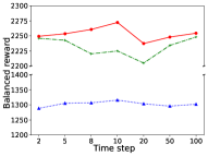
(a) Ratio 0.1 on IHDP

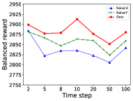
(b) Ratio 0.1 on JOBS

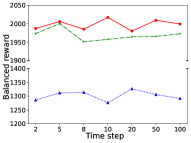
(c) Ratio 0.4 on IHDP

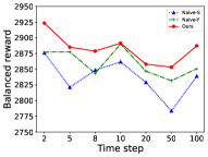
(d) Ratio 0.4 on JOBS

Figure 3: Comparison of Naive-S, Naive-Y and our method with different time steps and other fixed missing ratios $\{0.2,0.4\}$ on IHDP and JOBS.

Appendix E Data Generation Details of $Y$ for $S\perp\!\!\!\perp Y|X$

To generate long-term outcomes $Y_{i}(0)$ and $Y_{i}(1)$ such that $S\perp\!\!\!\perp Y|X$, for IHDP, we set the initial value at time step $0$ as $Y_{0,i}(0)\sim\mathrm{Bern}(\sigma(w_{0}X_{i}+\epsilon_{0,i})),S_{i}(1)\sim\mathrm{Bern}(\sigma(w_{1}X_{i}+\epsilon_{1,i}))$, other than $Y_{0,i}(0)=S_{i}(0),Y_{0,i}(1)=S_{i}(1)$. For JOBS, we generate $Y$ with $Y\perp\!\!\!\perp S|X$ in the following way, $Y_{t,i}(0)\sim\mathrm{Bern}(\sigma(\beta_{0}X_{i}))+\epsilon_{0,i},Y_{t,i}(1)\sim\mathrm{Bern}(\sigma(\beta_{1}X_{i}))+\epsilon_{1,i}$. Parameter values remain unchanged unless specified. Both ways for two datasets break the correlated relationships between $S$ and $Y$ given $X$.

References

• Athey et al. (2019a) Athey, S., Chetty, R., Imbens, G., and Kang, H. The surrogate index: Combining short-term proxies to estimate long-term treatment effects more rapidly and precisely. Working paper, National Bureau of Economic Research, 2019a.
• Athey et al. (2019b) Athey, S., Tibshirani, J., and Wager, S. Generalized random forests. The Annals of Statistics, 47:1148–1178, 2019b.
• Athey et al. (2020) Athey, S., Chetty, R., and Imbens, G. Combining experimental and observational data to estimate treatment effects on long term outcomes. arXiv preprint arXiv:2006.09676, 2020.
• Ben-Michael et al. (2022) Ben-Michael, E., Imai, K., and Jiang, Z. Policy learning with asymmetric utilities. arXiv preprint arXiv:2206.10479, 2022.
• Bertsimas et al. (2016) Bertsimas, D., Kallus, N., Weinstein, A. M., and Zhuo, Y. D. Personalized Diabetes Management Using Electronic Medical Records. Diabetes Care, 40:210–217, 2016.
• Chen et al. (2016) Chen, G., Zeng, D., and Kosorok, M. R. Personalized dose finding using outcome weighted learning. Journal of the American Statistical Association, 111:1509–1521, 2016.
• Chen et al. (2007) Chen, H., Geng, Z., and Jia, J. Criteria for surrogate end points. Journal of the Royal Statistical Society: Series B (Statistical Methodology), 69:919–932, 2007.
• Chen & Ritzwoller (2021) Chen, J. and Ritzwoller, D. M. Semiparametric estimation of long-term treatment effects. arXiv preprint arXiv:2107.14405, 2021.
• Cheng et al. (2021) Cheng, L., Guo, R., and Liu, H. Long-term effect estimation with surrogate representation. In Proceedings of the 14th ACM International Conference on Web Search and Data Mining, pp.  274–282, 2021.
• Chernozhukov et al. (2018) Chernozhukov, V., Chetverikov, D., Demirer, M., Duflo, E., Hansen, C., Newey, W., and Robins, J. Double/debiased machine learning for treatment and structural parameters. The Econometrics Journal, 21:1–68, 2018.
• Chetty et al. (2007) Chetty, R., Friedman, J. N., Hilger, N., Saez, E., Schanzenbach, D. W., and Yagan, D. How does your kindergarten classroom affect your earnings? evidence from project star. The Quarterly Journal of Economics, 126:1593–1660, 2007.
• Chiappa (2019) Chiappa, S. Path-specific counterfactual fairness. In Proceedings of the AAAI Conference on Artificial Intelligence, 2019.
• Correa et al. (2019) Correa, J. D., Tian, J., and Bareinboim, E. Identification of causal effect in the presence of selection bias. In Proceedings of the Thirty-Third AAAI Conference on Artificial Intelligence, 2019.
• Dudík et al. (2011) Dudík, M., Langford, J., and Li, L. Doubly robust policy evaluation and learning. In Proceedings of the 28th International Conference on International Conference on Machine Learning, pp.  1097–1104. PMLR, 2011.
• Fang et al. (2023) Fang, E. X., Wang, Z., and Wang, L. Fairness-oriented learning for optimal individualized treatment. Journal of the American Statistical Association, 118:1733–1746, 2023.
• Fleming et al. (1994) Fleming, T. R., Prentice, R. L., Pepe, M. S., and Glidden, D. Surrogate and auxiliary endpoints in clinical trials, with potential applications in cancer and aids research. Journal of the Royal Statistical Society: Series B (Statistical Methodology), 13:955–968, 1994.
• Floridi (2019) Floridi, L. Establishing the rules for building trustworthy ai. Nature Machine Intelligence, 1:261–262, 2019.
• Frangakis & Rubin (2002) Frangakis, C. E. and Rubin, D. B. Principal stratification in causal inference. Biometrics, 58:21–29, 2002.
• Hernán & Robins (2020) Hernán, M. and Robins, J. M. Causal Inference: What If. Boca Raton: Chapman and Hall/CRC, 2020.
• Hill (2011) Hill, J. L. Bayesian nonparametric modeling for causal inference. Journal of Computational and Graphical Statistics, 20:217–240, 2011.
• Hohnhold et al. (2015) Hohnhold, H., O’Brien, D., and Tang, D. Focusing on the long-term: It’s good for users and business. In Proceedings of the 21th ACM SIGKDD International Conference on Knowledge Discovery and Data Mining, 2015.
• Holland (1986) Holland, P. W. Statistics and causal inference. Journal of the American Statistical Association, 81:945–960, 1986.
• Hu et al. (2023) Hu, W., Zhou, X.-H., and Wu, P. Identification and estimation of treatment effects on long-term outcomes in clinical trials with external observational data. Statistica Sinica, 2023.
• Imbens et al. (2022) Imbens, G., Kallus, N., Mao, X., and Wang, Y. Long-term causal inference under persistent confounding via data combination. arXiv preprint 2202.07234, 2022.
• Imbens & Rubin (2015) Imbens, G. W. and Rubin, D. B. Causal Inference For Statistics Social and Biomedical Science. Cambridge University Press, 2015.
• Ju & Geng (2010) Ju, C. and Geng, Z. Criteria for surrogate end points based on causal distributions. Journal of the Royal Statistical Society: Series B, 72:129–142, 2010.
• Kallus (2022a) Kallus, N. Treatment effect risk: Bounds and inference. In 2022 ACM Conference on Fairness, Accountability, and Transparency, FAccT ’22, pp.  213, New York, NY, USA, 2022a. Association for Computing Machinery.
• Kallus (2022b) Kallus, N. What’s the harm? sharp bounds on the fraction negatively affected by treatment. arXiv preprint arXiv:2205.10327, 2022b.
• Kallus & Mao (2020) Kallus, N. and Mao, X. On the role of surrogates in the efficient estimation of treatment effects with limited outcome data. arXiv:2003.12408, 2020.
• Kallus & Zhou (2018) Kallus, N. and Zhou, A. Confounding-robust policy improvement. In NeurIPS, 2018.
• Kaur et al. (2022) Kaur, D., Uslu, S., Rittichier, K. J., and Durresi, A. Trustworthy artificial intelligence: a review. ACM Computing Surveys (CSUR), 55:1–38, 2022.
• Kitagawa & Tetenov (2018) Kitagawa, T. and Tetenov, A. Who should be treated? empirical welfare maximization methods for treatment choice. Econometrica, 86, 2018.
• Kohavi et al. (2012) Kohavi, R., Deng, A., Frasca, B., Longbotham, R., Walker, T., and Xu, Y. Trustworthy online controlled experiments: five puzzling outcomes explained. In Proceedings of the 18th ACM SIGKDD international conference on Knowledge discovery and data mining, 2012.
• Kosorok & Laber (2019) Kosorok, M. R. and Laber, E. B. Precision medicine. Annual Review of Statistics and Its Application, 6:263–86, 2019.
• Kusner et al. (2017) Kusner, M. J., Loftus, J., Russell, C., and Silva, R. Counterfactual fairness. Advances in neural information processing systems, 30, 2017.
• LaLonde (1986) LaLonde, R. J. Evaluating the econometric evaluations of training programs with experimental data. The American economic review, pp.  604–620, 1986.
• Lauritzen et al. (2004) Lauritzen, S. L., Aalen, O. O., Rubin, D. B., and Arjas, E. Discussion on causality [with reply]. Scandinavian Journal of Statistics, 31:189–201, 2004.
• Li et al. (2023) Li, H., Zheng, C., Cao, Y., Geng, Z., Liu, Y., and Wu, P. Trustworthy policy learning under the counterfactual no-harm criterion. In International Conference on Machine Learning, pp. 20575–20598. PMLR, 2023.
• Murphy (2003) Murphy, S. A. Optimal dynamic treatment regimes. Journal of the Royal Statistical Society: Series B (Statistical Methodology), 65:331–355, 2003.
• Nabi & Shpitser (2018) Nabi, R. and Shpitser, I. Fair inference on outcomes. In Proceedings of the AAAI Conference on Artificial Intelligence, 2018.
• Newey (1990) Newey, W. K. Semiparametric efficiency bounds. Journal of Applied Econometrics, 5:99–135, 1990.
• Neyman (1990) Neyman, J. S. On the application of probability theory to agricultural experiments. essay on principles. section 9. Statistical Science, 5:465–472, 1990.
• Prentice (1989) Prentice, R. L. Surrogate endpoints in clinical trials: definition and operational criteria. Statistics in medicine, 8:431–440, 1989.
• Puterman (2014) Puterman, M. L. Markov decision processes: discrete stochastic dynamic programming. John Wiley & Sons, 2014.
• Qiu et al. (2021) Qiu, H., Carone, M., Sadikova, E., Petukhova, M., Kessler, R. C., and Luedtke, A. Optimal individualized decision rules using instrumental variable methods. Journal of the American Statistical Association, 116:174–191, 2021.
• Rubin (1974) Rubin, D. B. Estimating causal effects of treatments in randomized and nonrandomized studies. Journal of educational psychology, 66:688–701, 1974.
• Semenova & Chernozhukov (2021) Semenova, V. and Chernozhukov, V. Debiased machine learning of conditional average treatment effects and and other causal functions. The Econometrics Journal, 24:264–289, 2021.
• Shapiro (1991) Shapiro, A. Asymptotic analysis of stochastic programs. Annals of Operations Research, 30:169–186, 1991.
• Sutton & Barto (2018) Sutton, R. S. and Barto, A. G. Reinforcement learning: An introduction. MIT press, 2018.
• Thiebes et al. (2021) Thiebes, S., Lins, S., and Sunyaev, A. Trustworthy artificial intelligence. Electronic Markets, 31:447–464, 2021.
• Tsiatis (2006) Tsiatis, A. A. Semiparametric Theory and Missing Data. Springer, 2006.
• van der Vaart (1998) van der Vaart, A. W. Asymptotic statistics. Cambridge University Press, 1998.
• Wager & Athey (2018) Wager, S. and Athey, S. Estimation and inference of heterogeneous treatment effects using random forests. Journal of the American Statistical Association, 113:1228–1242, 2018.
• Wang et al. (2021) Wang, W., Feng, F., He, X., Zhang, H., and Chua, T.-S. Clicks can be cheating: Counterfactual recommendation for mitigating clickbait issue. In Proceedings of the 44th International ACM SIGIR Conference on Research and Development in Information Retrieval, 2021.
• Wang et al. (2018) Wang, Y., Fu, H., and Zeng, D. Learning optimal personalized treatment rules in consideration of benefit and risk: With an application to treating type 2 diabetes patients with insulin therapies. Journal of the American Statistical Association, 113:1–13, 2018.
• Wu et al. (2019) Wu, Y., Zhang, L., Wu, X., and Tong, H. PC-Fairness: A unified framework for measuring causality-based fairness. Advances in Neural Information Processing Systems, 32, 2019.
• Yang et al. (2023a) Yang, J., Eckle, D., Dhillon, P., and Aral, S. Targeting for long-term outcomes. Management Science, Online:https://pubsonline.informs.org/doi/10.1287/mnsc.2023.4881, 2023a.
• Yang et al. (2023b) Yang, J., Eckles, D., Dhillon, P., and Aral, S. Targeting for long-term outcomes. Management Science, 2023b.
• Yin et al. (2020) Yin, Y., Liu, L., Geng, Z., and Luo, P. Novel criteria to exclude the surrogate paradox and their optimalities. Scandinavian Journal of Statistics, 47:84–103, 2020.
• Zhao et al. (2012) Zhao, Y., Zeng, D., Rush, A. J., and Kosorok, M. R. Estimating individualized treatment rules using outcome weighted learning. Journal of the American Statistical Association, 104:1106–1118, 2012.