A continuous approach for computing the pseudospectra of linear operators

Abstract

We propose a continuous approach for computing the pseudospectra of linear operators following a “solve-then-discretize” strategy. Instead of taking a finite section approach or using a finite-dimensional matrix to approximate the operator of interest, the new method employs an operator analogue of the Lanczos process to work with operators and functions directly. The method is shown to be free of spectral pollution and spectral invisibility, fully adaptive, nearly optimal in accuracy, and well-conditioned. The advantages of the method are demonstrated by extensive numerical examples and comparison with the traditional method.

65F15, 15A18, 47A10, 47E05, 47G10

1 Introduction

In his 1999 Acta Numerica paper [36], Trefethen wrote,

This field (the computation of pseudospectra) will also participate in a broader trend in the scientific computing of the future, the gradual breaking down of the walls between the two steps of discretization (operator $\longrightarrow$ matrix) and solution (matrix $\longrightarrow$ spectrum or pseudospectra).

Not only serving as a projection for the future, this sentence also succinctly encapsulates the standard routine for computing the pseudospectra of an operator some 25 years ago. At the time of writing, it is still the default approach for the task. It begins by approximating a linear operator $\mathcal{L}$, e.g., a differential operator, using a discretization method, e.g., a spectral method. If we denote by $L$ this finite-dimensional matrix approximation of $\mathcal{L}$, the pseudospectra of $\mathcal{L}$ at $z\in\mathbb{C}$ is then approximated by that of $L$ following the definition of the $\varepsilon$-pseudospectrum of a matrix

(1) $$\sigma_{\varepsilon}(L)=\left\{z\in\mathbb{C}\mid\|(zI-L)^{-1}\|>\varepsilon^{-1}\right\},$$

where $I$ is the identity. In case of $z$ being an eigenvalue of $L$, we take the convention that $\|(z\mathcal{I}-L)^{-1}\|=\infty$. If $2$-norm is adopted, Eq. 1 amounts to the computation of the smallest singular value of $zI-L$

$$\sigma_{\varepsilon}(L)=\{z\in\mathbb{C}\mid s_{\min}(zI-L)<\varepsilon\}.$$

The standard method for calculating the pseudospectra of a matrix is the core EigTool algorithm [37, §39], which is recapitulated in Algorithm 1.

Algorithm 1 Core EigTool algorithm

0:  A matrix $L\in\mathbb{C}^{n\times n}$, $z\in\mathbb{C}$, a normalized vector $u_{1}\in\mathbb{C}^{n}$, a tolerance $\delta$

1:  Compute the Schur form $\tilde{L}$ so that $L$ and $\tilde{L}$ are unitarily similar.

2:  repeat

3:     Perform Lanczos iteration $T(z)U_{k}=U_{k}H_{k}+\beta_{k+1}u_{k+1}e_{k}^{T}$, where $T(z)=(zI-\tilde{L})^{-*}(zI-\tilde{L})^{-1}$, $U_{k}=[u_{1},\dots,u_{k}]\in\mathbb{C}^{n\times k}$, and $u_{k+1}\in\mathbb{C}^{n}$, to obtain the symmetric tridiagonal matrix $H_{k}\in\mathbb{R}^{k\times k}$.

4:     Compute the largest Ritz value $\mu_{1}^{(k)}=\lambda_{1}(H_{k})$.

5:     $k\leftarrow k+1$

6:  until $|\mu_{1}^{(k)}/\mu_{1}^{(k-1)}-1|<\delta$

6:  $\lVert(zI-L)^{-1}\rVert=\sqrt{\mu_{1}^{(k)}}$.

This “discretize-then-solve” paradigm has a few drawbacks: (1) There is no guarantee that the pseudospectra of $L$ serves as a quality approximation to that of the original operator, since $L$ is only of finite dimension. More importantly, the computation may suffer from the so-called spectral pollution, i.e., spurious eigenvalues and pseudospectra, and spectral invisibility, i.e., missing parts of the spectrum and pseudospectra. See Section 5.2 for an example. This is known as the “finite section” caveat [16]. (2) It is difficult to effect adaptivity. (3) $T(z)$ could be more ill-conditioned than the original problem is. See Section 5.3 for an example. (4) Even though spectral approximation to the operators are used, the convergence of the resolvent norm may fall short of spectral in terms of the degrees of freedom (DoF) [37, §43]. See also Section 5.3 for an example.

More recently, computing the pseudospectra of general bounded infinite matrices is addressed in [16], followed by a significantly improved version [6, 8] that offers a rigorous error control and the ability to deal with a greater range of problems, such as partial differential operators in unbounded domains. It is proposed to represent an operator $\mathcal{L}$ as a matrix of infinite dimension that acts on $\ell^{2}(\mathbb{N})$. For a sequence of nested operator foldings and rectangular truncations of this infinite matrix, the limit of the smallest singular value is shown to be $\lVert(z\mathcal{I}-\mathcal{L})^{-1}\rVert^{-1}$. This iterative method nevertheless also lacks adaptivity in stopping criterion and may have difficulty in dealing with operators equipped with boundary conditions, e.g., differential operators in compact domains.

This paper shows that the pseudospectra of operators can be computed following a “solve-then-discretize” strategy [5, 7, 9, 11, 19] by taking advantage of the recent development in spectral methods. The new method is an operator analogue of the Lanczos process that computes with operators and functions directly. This leads to a number of advantages: (1) We use effectively infinite-dimensional matrix representation of the operators, which rules out spectral pollution and spectral invisibility. (2) The computation is fully adaptive for nearly optimal accuracy justified by an a priori analysis. (3) We use the recently developed sparse or structured spectral methods which are well-conditioned, making the most of the floating-point precision. (4) No involvement of quadrature or weight matrices, and the convergence is spectral. More importantly, the new method offers a unified framework for computing the pseudospectra of linear operators. Though we confine ourselves in this article with certain spectral methods only, any method for solving the inverse resolvent equations corresponding to the operator of interest (see Eq. 12) can be incorporated straightforwardly in a plug-and-play fashion.

Throughout this paper, we assume $\mathcal{L}:\mathcal{D}(\mathcal{L})\subseteq\mathcal{H}\rightarrow\mathcal{H}$ be a closed linear operator on a separable Hilbert space $\mathcal{H}$. For $z\in\mathbb{C}$, the resolvent of $\mathcal{L}$ at $z$ is the operator

$$\mathcal{R}(z)=(z\mathcal{I}-\mathcal{L})^{-1},$$

given that $\mathcal{R}(z)\in\mathcal{B}(\mathcal{H})$ exists, where $\mathcal{B}(\mathcal{H})$ denotes the set of bounded operators on $\mathcal{H}$. For $\varepsilon>0$, the $\varepsilon$-pseudospectrum of $\mathcal{L}$ is

(2) $$\sigma_{\varepsilon}(\mathcal{L})=\left\{z\in\mathbb{C}\mid\|(z\mathcal{I}-\mathcal{L})^{-1}\|>\varepsilon^{-1}\right\},$$

with the convention $\|(z\mathcal{I}-\mathcal{L})^{-1}\|=\infty$ if $z\in\sigma(\mathcal{L})$, where $\sigma(\mathcal{L})$ denotes the spectrum of $\mathcal{L}$. This definition can be found in, for example, [37, §4].

In the remainder of this paper, $\|\cdot\|=\|\cdot\|_{2}$, induced by the Euclidean inner product, unless indicated otherwise. We use $\langle\cdot,\cdot\rangle$ to denote the inner product. $\Lambda(\cdot)$ and $\sigma(\cdot)$ are used to denote the set of eigenvalues and the spectrum of an operator. The largest eigenvalue, if exists and is isolated, is denoted by $\lambda_{1}(\cdot)$. $\Re(\cdot)$ stands for the real part of a complex number. $\mathcal{I}$ and $I_{\infty}$ are respectively the identity operator and infinite-dimensional identity matrix. An asterisk is used to denote the complex conjugate of a complex variable and the adjoint of an operator. We denote by $\epsilon_{mach}$ the machine epsilon, which is, for example, about $2.22\times 10^{-16}$ in the double precision floating point arithmetic.

The paper is structured as follows. In Section 2, we introduce the operator analogue of the core EigTool algorithm. Section 3 gives the details of the implementation, where we show that the method is adaptive in resolution and quadrature-free using proper spectral methods. In Section 4, we discuss the convergence and supply a careful error analysis which leads to an adaptive stopping criterion for the continuous Lanczos process. We test the method in Section 5 with extensive experiments before demonstrating a few important extensions in Section 6. Section 7 closes by a summary.

2 Operator analogue of the core EigTool algorithm

The definition Eq. 2 offers limited guidance on the practical computation of an operator’s pseudospectra. To relate the norm in Eq. 2 to a computable quantity, we note that

$$\lVert(z\mathcal{I}-\mathcal{L})^{-1}\rVert^{2}=\lVert\mathcal{R}^{*}(z)\mathcal{R}(z)\rVert=\sup\sigma(\mathcal{R}^{*}(z)\mathcal{R}(z)).$$

If $\lVert\mathcal{R}^{*}(z)\mathcal{R}(z)\rVert$ happens to be the largest eigenvalue and is isolated, i.e,

(3) $$\sup\sigma(\mathcal{R}^{*}(z)\mathcal{R}(z))=\lambda_{1}(\mathcal{R}^{*}(z)\mathcal{R}(z)),$$

Algorithm 1 can be generalized to deal with $\mathcal{L}$. Algorithm 2 is the operator analogue of the core EigTool algorithm, where the computation of the pseudospectra of an operator $\mathcal{L}$ boils down to finding the largest eigenvalue of $\mathcal{T}(z)=\mathcal{R}^{*}(z)\mathcal{R}(z)$.

Algorithm 2 The operator analogue of the core EigTool algorithm

0:  A linear operator $\mathcal{L}:\mathcal{D}(\mathcal{L})\rightarrow\mathcal{H}$, $z\in\mathbb{C}$, a normalized function $u_{1}\in\mathcal{H}$, a tolerance $\delta$

1:  repeat

2:     Perform $k$th Lanczos iteration (Algorithm 3)

(4) $$\mathcal{T}(z)\mathcal{U}_{k}=\mathcal{U}_{k}H_{k}+\beta_{k+1}u_{k+1}e_{k}^{T},$$

where $\mathcal{T}(z)=(z\mathcal{I}-\mathcal{L})^{-*}(z\mathcal{I}-\mathcal{L})^{-1}$, $\mathcal{U}_{k}=(u_{1}|\cdots|u_{k})$, and $u_{1},\dots,u_{k+1}\in\mathcal{H}$, to obtain the symmetric tridiagonal matrix $H_{k}\in\mathbb{R}^{k\times k}$.

3:     Compute the largest Ritz value $\mu_{1}^{(k)}=\lambda_{1}(H_{k})$ and the corresponding eigenvector $y_{1}^{(k)}=[y_{11}^{(k)},\dots,y_{k1}^{(k)}]^{T}\in\mathbb{R}^{n}$.

4:     $k\leftarrow k+1$

5:  until $\beta_{k+1}|y_{k1}^{(k)}|<(\mu_{1}^{(k)})^{3/2}\delta$

5:  $\lVert(z\mathcal{I}-\mathcal{L})^{-1}\rVert=\sqrt{\mu_{1}^{(k)}}$.

The most notable distinction of Algorithm 2 from Algorithm 1 lies in the substitution of matrix $L$ with the operator $\mathcal{L}$. Additionally, there are two minor changes relative to Algorithm 1. Firstly, the preliminary triangularization (line 1 of Algorithm 1), which is instrumental in reducing the computational cost [22], has been omitted. Secondly, a new stopping criterion is introduced in line 5 and further elaborated upon in Sections 3.2 and 4.2.

Now we wonder for what kind of linear operator $\mathcal{L}$ Eq. 3 holds so that the pseudospectra of $\mathcal{L}$ can be computed by Algorithm 2. The following lemma shows that this is the case, provided that the resolvent $\mathcal{R}(z)$ is compact or compact-plus-scalar.

Lemma 2.1.

(1) If $\mathcal{R}(z)$ is compact, $\sup\sigma(\mathcal{T}(z))=\lambda_{1}(\mathcal{T}(z))$. (2) If $\mathcal{R}(z)$ is compact-plus-scalar, i.e., $\mathcal{R}(z)=\mathcal{K}+\zeta\mathcal{I}$, where $\zeta\in\mathbb{C}$ and $\mathcal{K}$ is compact on $\mathcal{H}$, then $\sup\sigma(\mathcal{T}(z))=\lambda_{1}(\mathcal{T}(z))$, except the case $\sup\sigma(\mathcal{T}(z))=|\zeta|^{2}$.

Proof 2.2.

(1) follows from the fact that $\mathcal{T}(z)=\mathcal{R}(z)^{*}\mathcal{R}(z)$ is a compact self-adjoint operator and the spectral theorem [12, §4.5]. To show (2), let

$$\mathcal{T}(z)=(\mathcal{K}+\zeta\mathcal{I})^{*}(\mathcal{K}+\zeta\mathcal{I})=\mathcal{J}+|\zeta|^{2}\mathcal{I},$$

where $\mathcal{J}=\zeta\mathcal{K}^{*}+\zeta^{*}\mathcal{K}+\mathcal{K}^{*}\mathcal{K}$. Noting that $\mathcal{J}$ is a compact self-adjoint operator, we use the spectral theorem again to have

$$\sup\sigma(\mathcal{T}(z))=\sup\Lambda(\mathcal{J})+|\zeta|^{2},$$

where $\Lambda(\mathcal{J})$ forms a real countably infinite sequence with a unique accumulation point at $0$. When $\sup\Lambda(\mathcal{J})\neq 0$, $\sup\sigma(\mathcal{T}(z))=\lambda_{1}(\mathcal{J})+|\zeta|^{2}=\lambda_{1}(\mathcal{T}(z))$.

The results we collect or show in the following subsections reveal that virtually all of the common linear operators have compact or compact-plus-scalar resolvent. These include differential operators restricted by proper boundary conditions and integral operators of Volterra and Fredholm types, which we now discuss individually. In addition, we also give the detail for formulating $\mathcal{R}^{*}(z)$ for each operator.

2.1 Differential operators

For the differential expression

$$\tau=\frac{\mathrm{d}^{N}}{\mathrm{d}x^{N}}+a_{N-1}(x)\frac{\mathrm{d}^{N-1}}{\mathrm{d}x^{N-1}}+\cdots+a_{1}(x)\frac{\mathrm{d}}{\mathrm{d}x}+a_{0}(x),$$

where $a_{k}(x)$ for $k=0,1,\ldots,N-1$ are locally integrable on $[a,b]$, the maximal operator $\mathcal{Q}_{\max}:L^{2}([a,b])\rightarrow L^{2}([a,b])$ is defined by $\mathcal{Q}_{\max}g=\tau g$ with $\mathcal{D}\left(\mathcal{Q}_{\max}\right)=\{g\in\mathcal{A}\mathcal{C}_{N}([a,b])\cap L^{2}([a,b])\mid\tau g\in L^{2}([a,b])\}$. Suppose that $\mathcal{Q}$ is a restriction of $\mathcal{Q}_{\max}$ by proper boundary conditions [13, §XIV.3]. It can be shown that $\mathcal{R}(z)=(z\mathcal{I}-\mathcal{Q})^{-1}$ is compact for $z\in\mathbb{C}\backslash\sigma(\mathcal{Q})$ [13, §XIV.3]. For $\mathcal{R}^{*}(z)$, we use the fact $(z\mathcal{I}-\mathcal{Q})^{-*}=(z^{*}\mathcal{I}-\mathcal{Q}^{*})^{-1}$, where $\mathcal{Q}^{*}$ can be found by definition. See, for example, [13, §XIV.4].

2.2 Fredholm integral operator

The Fredholm integral operator $\mathcal{F}:L^{2}([a,b])\rightarrow L^{2}([a,b])$ is defined as

(5) $$(\mathcal{F}u)(s)=\int_{a}^{b}K(s,t)u(t)\mathrm{d}t,\quad a\leq s\leq b,$$

where the kernel $K(s,t)\in L^{2}([a,b]\times[a,b])$. For any nonzero $z\in\mathbb{C}$ that is not an eigenvalue of $\mathcal{F}$, $\mathcal{R}(z)=(z\mathcal{I}-\mathcal{F})^{-1}$ is compact-plus-scalar [30, Theorem 2.1.2]. To evaluate $\mathcal{R}^{*}(z)$, we use $(z\mathcal{I}-\mathcal{F})^{-*}=(z^{*}\mathcal{I}-\mathcal{F}^{*})^{-1}$, where $(\mathcal{F}^{*}u)(s)=\int_{a}^{b}K^{*}(t,s)u(t)\mathrm{d}t$.

One of the most important subcases of the Fredholm integral operator is the Fredholm convolution integral operator

(6) $$(\mathcal{F}_{c}u)(s)=\int_{a}^{b}K(s-t)u(t)\mathrm{d}t,\quad a\leq s\leq b.$$

2.3 Volterra integral operator

The Volterra integral operator $\mathcal{V}:L^{2}([a,b])\rightarrow L^{2}([a,b])$ given by

(7) $$(\mathcal{V}u)(s)=\int_{a}^{s}K(s,t)u(t)\mathrm{d}t,\quad a\leq s\leq b$$

can be deemed as a subcase of the Fredholm integral operator [30, §2.7] with the kernel $K(s,t)\in L^{2}([a,b]\times[a,b])$ zero-valued for $a\leq s<t\leq b$. For any nonzero $z\in\mathbb{C}$, $\mathcal{R}(z)=(z\mathcal{I}-\mathcal{V})^{-1}$ is compact-plus-scalar [30, Theorem 2.7.1]. For $\mathcal{R}^{*}(z)$, we use the fact that $(z\mathcal{I}-\mathcal{V})^{-*}=(z^{*}\mathcal{I}-\mathcal{V}^{*})^{-1}$, where $(\mathcal{V}^{*}u)(s)=\int_{s}^{b}K^{*}(t,s)u(t)\mathrm{d}t$. Similarly, an important subcase of the Volterra integral operator is the Volterra convolution integral operator

(8) $$(\mathcal{V}_{c}u)(s)=\int_{a}^{s}K(s-t)u(t)\mathrm{d}t,\quad a\leq t\leq s\leq b.$$

2.4 Generalized eigenvalue problem

For the generalized eigenvalue problem (GEP)

(9) $$\mathcal{A}x=\lambda\mathcal{B}x,$$

we consider the case where both $\mathcal{A}$ and $\mathcal{B}$ are differential operators defined in Section 2.1 subject to proper boundary conditions so that $\mathcal{B}$ is invertible and $\mathcal{D}(\mathcal{A})\subset\mathcal{D}(\mathcal{B})$. Specifically, we assume that $\mathcal{A}$ and $\mathcal{B}$ have respectively the differential expressions

$$\tau_{\mathcal{A}} =\frac{\mathrm{d}^{N}}{\mathrm{d}x^{N}}+a_{N-1}(x)\frac{\mathrm{d}^{N-1}}{\mathrm{d}x^{N-1}}+\cdots+a_{1}(x)\frac{\mathrm{d}}{\mathrm{d}x}+a_{0}(x),$$

$$\tau_{\mathcal{B}} =b_{M}(x)\frac{\mathrm{d}^{M}}{\mathrm{d}x^{M}}+b_{M-1}(x)\frac{\mathrm{d}^{M-1}}{\mathrm{d}x^{M-1}}+\cdots+b_{1}(x)\frac{\mathrm{d}}{\mathrm{d}x}+b_{0}(x).$$

Without loss of generality, we also assume $M<N$. If we denote by $\Lambda(\mathcal{A},\mathcal{B})=\{\lambda\in\mathbb{C}\mid\mathcal{A}x=\lambda\mathcal{B}x,\ x\neq 0\}$ the set of eigenvalues of Eq. 9, Eq. 9 can be solved as the standard eigenvalue problem with $\Lambda(\mathcal{A},\mathcal{B})=\Lambda(\mathcal{G})$ by the invertibility of $\mathcal{B}$, where $\mathcal{G}=\mathcal{B}^{-1}\mathcal{A}$. Moreover, this is followed by the $\varepsilon$-pseudospectrum of the GEP

$$\sigma_{\varepsilon}(\mathcal{A},\mathcal{B})=\sigma_{\varepsilon}\left(\mathcal{G}\right),$$

which is the operator extension of the definition for the pseudospectra of matrix GEPs [37, §45].

Lemma 2.3.

For the GEP Eq. 9, we further assume that $a_{j}(x),b_{k}(x)\in L^{\infty}([a,b])$ for $j=0,1,\ldots,N-1$ and $k=0,1,\ldots,M$ respectively and $\mathcal{D}(\mathcal{A}^{*})\subset\mathcal{D}(\mathcal{B}^{*})$. Then (1) $\mathcal{R}(z)=(z\mathcal{I}-\mathcal{G})^{-1}$ and

(10a) $$\mathcal{R}^{*}(z)=\mathcal{B}^{*}(z^{*}\mathcal{B}^{*}-\mathcal{A}^{*})^{-1}$$

are both compact for $$z\in\mathbb{C}\backslash\sigma(\mathcal{G}) \mathcal{R}(z) \mathcal{D}(\mathcal{B}_{\max})$$; (2) the restriction of to is

(10b) $$\mathcal{R}(z)\big{|}_{\mathcal{D}(\mathcal{B}_{\max})}=(z\mathcal{B}-\mathcal{A})^{-1}\mathcal{B}_{\max}.$$

Proof 2.4.

We note that $(z\mathcal{I}-\mathcal{G})^{*}=(z^{*}\mathcal{B}^{*}-\mathcal{A}^{*})\mathcal{B}^{-*}$, and its domain $\mathcal{D}((z\mathcal{I}-\mathcal{G})^{*})=\{u\in L^{2}([a,b])\arrowvert\mathcal{B}^{-*}u\in\mathcal{D}(\mathcal{A}^{*})\}$. When $z^{*}\mathcal{B}^{*}-\mathcal{A}^{*}$ is invertible, so is $(z\mathcal{I}-\mathcal{G})^{*}$, and $\mathcal{R}^{*}(z)=\left((z\mathcal{I}-\mathcal{G})^{-1}\right)^{*}=\left((z\mathcal{I}-\mathcal{G})^{*}\right)^{-1}=\mathcal{B}^{*}(z^{*}\mathcal{B}^{*}-\mathcal{A}^{*})^{-1}$ by Proposition 2.6 in [13, §XIV.2]. Since $\{a_{k}\}_{k=0}^{N-1},\{b_{k}\}_{k=0}^{M}\in L^{\infty}([a,b])$ and $M<N$, $\mathcal{B}^{*}$ is $(z^{*}\mathcal{B}^{*}-\mathcal{A}^{*})$-compact by Theorem 1.3 in [13, §XVII.1]. It then follows from the invertibility of $z^{*}\mathcal{B}^{*}-\mathcal{A}^{*}$ and the argument used in the proof of Theorem 5.1 in [13, §XVII.5] that $\mathcal{B}^{*}(z^{*}\mathcal{B}^{*}-\mathcal{A}^{*})^{-1}$ is compact, i.e., $\mathcal{R}^{*}(z)$ is compact, which, in turn, leads to the compactness of $\mathcal{R}(z)$.

To show (2), we first consider $\mathcal{R}(z)\big{|}_{\mathcal{D}(\mathcal{B})}$. For $\phi\in\mathcal{D}(\mathcal{B})$ and $\psi\in L^{2}([a,b])$,

(11) $$\langle(z\mathcal{B}-\mathcal{A})^{-1}\mathcal{B}\phi,\psi\rangle=\langle\mathcal{B}\phi,(z^{*}\mathcal{B}^{*}-\mathcal{A}^{*})^{-1}\psi\rangle=\langle\phi,\mathcal{B}^{*}(z^{*}\mathcal{B}^{*}-\mathcal{A}^{*})^{-1}\psi\rangle,$$

from which it follows that $\mathcal{R}(z)\big{|}_{\mathcal{D}(\mathcal{B})}=(z\mathcal{B}-\mathcal{A})^{-1}\mathcal{B}$. By the extension theorem for bounded linear operators, we have $\mathcal{R}(z)\big{|}_{\mathcal{D}(\mathcal{B}_{\max})}=(z\mathcal{B}-\mathcal{A})^{-1}\mathcal{B}_{\max}$.

When evaluate $\mathcal{R}(z)$ and $\mathcal{R}^{*}(z)$ by Eq. 10b and Eq. 10a respectively, we need to know $\mathcal{A}^{*}$ and $\mathcal{B}^{*}$, which can be figured out as for the differential operators in Section 2.1.

3 Implementation

In this section, we focus on the practical implementation of lines 2 and 5 of Algorithm 2, i.e., the Lanczos process (Section 3.1) and the stopping criterion (Section 3.2).

3.1 Application of $\mathcal{T}(z)$

To facilitate the discussion, we elaborate the Lanczos iteration in Algorithm 3, which can be embedded into Algorithm 2 at line 2 there.

Algorithm 3 Lanczos process

0:  $\mathcal{T}(z)$, $H_{k-1}$, $\beta_{k}$, $u_{k}$, $u_{k-1}$

1:  $w_{k}=\mathcal{T}(z)u_{k}$

2:  if $k>1$ then

3:     $p_{k}=w_{k}-\beta_{k}u_{k-1}$

4:  else

5:     $p_{k}=w_{k}$

6:  end if

7:  $\alpha_{k}=\Re(\langle u_{k},p_{k}\rangle)$

8:  $q_{k}=p_{k}-\alpha_{k}u_{k}$

9:  $\beta_{k+1}=\lVert q_{k}\rVert$

10:  $u_{k+1}=q_{k}/\beta_{k+1}$

10:  $H_{k}$, $\beta_{k+1}$, $u_{k+1}$

In line 1 of Algorithm 3, we need to apply $\mathcal{T}(z)=(z\mathcal{I}-\mathcal{L})^{-*}(z\mathcal{I}-\mathcal{L})^{-1}$ to $u\in\mathcal{H}$. This amounts to solving

(12a) $$(z\mathcal{I}-\mathcal{L})v =u,$$

(12b) $$(z^{*}\mathcal{I}-\mathcal{L}^{*})w =v$$

in sequence. For adequate resolution, we employ the coefficient-based spectral methods using Legendre polynomials, which all lead to linear systems of infinite dimensions. Of course, we are unable to numerically solve a linear system of infinite dimensions. What we can do is to determine the optimal truncation and compute the solution simultaneously. The computed solution is as if it were obtained by solving the infinite-dimensional system. The adaptivity in determining the truncation and thereby the DoF $n$ for obtaining adequately resolved solution can be effected by either evaluating the residual at little cost [23] or examining the formation of coefficient plateaus [1]. The justification for using Legendre polynomials comes from the fact that, under the Legendre basis, the $L^{2}$-norm and the Euclidean inner product equal precisely to the $l^{2}$-norm and the dot product of the coefficient vectors, respectively, except for a scaling factor. This correspondence facilitates a computation that dispenses with quadratures.

Any normalized vector would, in principle, serve as the initial iterate $u_{1}$ for the Lanczos process, whereas in practice we simply take $u_{1}=(1,0,0,\ldots)^{T}$. We find this latter choice easy to implement and uniformly well-performing.

Now we give the detail of the spectral method for each operator. Only Eq. 12a is discussed, and analogue is easily drawn for Eq. 12b. For the matrix representation of the adjoints, see also Section 6.4.

3.1.1 Differential operator

When $\mathcal{L}$ is a differential operator $\mathcal{Q}$ defined in Section 2.1, so is $\mathcal{L}^{*}$, and we solve Eq. 12 by the ultraspherical spectral method [23]. Specifically, we first approximate the variable coefficients $a_{N-1}(x),\ldots,a_{0}(x)$ by Legendre series of degrees $m^{a_{N-1}},\ldots,m^{a_{0}}$. The coefficients in these Legendre series can be obtained using the fast Legendre transform [15] with $m^{a_{N-1}},\ldots,m^{a_{0}}$ determined by, e.g., the chopping algorithm [1]. This way, the matrix representation of maximal operator $\mathcal{Q}_{\max}$ can be approximated by an infinite-dimensional banded matrix that maps from the Legendre basis to the ultraspherical basis of half-integer order. Incorporating the boundary condition of $\mathcal{Q}$ results in an infinite-dimensional almost-banded system which can be solved for optimally truncated solution using the adaptive QR [23].

3.1.2 Fredholm operator

When $\mathcal{L}$ is a general Fredholm operator $\mathcal{F}$ defined by Eq. 5, we first approximate the kernel $K(s,t)$ by a continuous analogue of the low-rank adaptive cross approximation [34], i.e.,

(13) $$K(s,t)\approx\sum_{j=1}^{k}f_{j}(s)g_{j}(t).$$

Here, $f_{j}$ and $g_{j}$ $(j=1,2,\ldots,k)$ are the Legendre series of degree $m^{f}$ and $m^{g}$ respectively. With Eq. 13, $z\mathcal{I}-\mathcal{F}$ acting on $v$ can be approximated as

$$\left(z\mathcal{I}-\mathcal{F}\right)v\approx zv(s)-\sum_{j=1}^{k}\langle g_{j}^{*}(t),v(t)\rangle f_{j}(s).$$

It then follows that the matrix representation of $z\mathcal{I}-\mathcal{F}$ can be approximated by an infinite-dimensional diagonal plus rank-$k$ semiseparable matrix

$$M_{\mathcal{F}}(z)=zI_{\infty}-CR^{*},$$

where $C=\left[C_{1},\cdots,C_{k}\right]\in\mathbb{C}^{\infty\times k}$ and $R=\left[R_{1},\cdots,R_{k}\right]\in\mathbb{C}^{\infty\times k}$. The top $m^{f}+1$ elements of $C_{j}$ are the coefficients of Legendre expansion of $f_{j}(s)$ and the rest of $C_{j}$ are zeros. Similarly, $R_{j}$ is zero except the first $m^{g}+1$ elements which store the Legendre coefficients of $g_{j}(t)$. Thus, only the top left $(m^{f}+1)\times(m^{g}+1)$ block and the diagonal of $M_{\mathcal{F}}$ are nonzero. The standard approach for solving such a diagonal-plus-semiseparable system is given by [3].

3.1.3 Fredholm convolution operator

When $\mathcal{L}$ is a Fredholm convolution integral operator $\mathcal{F}_{c}$ given by Eq. 6, we approximate the univariate kernel function $K(x)$ by a Legendre series of degree $m^{K}$. Then the matrix representation of $\mathcal{F}_{c}$ can be approximated by an infinite-dimensional matrix with only the upper skew-triangular part of the top left $(m^{K}+1)\times(m^{K}+1)$ block being nonzero. These nonzero entries can be obtained from the $m^{K}+1$ Legendre coefficients using a four-term recurrence formula [21]. Combining it with the infinite-dimensional scalar matrix gives the infinite-dimension arrow-shaped approximation of $z\mathcal{I}-\mathcal{F}_{c}$.

3.1.4 Volterra operator

In case of $\mathcal{L}$ being the Volterra operator $\mathcal{V}$ defined by Eq. 7, we follow the same strategy for handling the Fredholm operator by approximating the kernel $K(s,t)$ using the low-rank approximation Eq. 13 so that

$$(\mathcal{V}v)(s)\approx\sum_{j=1}^{k}f_{j}(s)\int_{a}^{s}g_{j}(t)v(t)dt.$$

The matrix representation of $z\mathcal{I}-\mathcal{V}$ can be approximated by an infinite-dimensional banded matrix

$$M_{\mathcal{V}}(z)=zI_{\infty}-\sum_{j=1}^{k}M_{\frac{1}{2}}[f_{j}]J_{[a,b]}M_{\frac{1}{2}}[g_{j}],$$

where $J_{[a,b]}$ is the indefinite integral matrix for Legendre series [32, §4.7] and $M_{\frac{1}{2}}[f_{j}]$ and $M_{\frac{1}{2}}[g_{j}]$ are the Legendre multiplication matrices [23, §3.1]. The resulting infinite system can be solved using the adaptive QR.

3.1.5 Volterra convolution operator

When $\mathcal{L}$ is a Volterra convolution integral operator $\mathcal{V}_{c}$ defined by Eq. 8, the kernel $K(x)$ is approximated by a Legendre series of degree $m^{K}$. With the coefficients of this Legendre series, a banded infinite-dimensional matrix can be constructed using a three-term recurrence formula [14, 38] to approximate the matrix representation of $z\mathcal{I}-\mathcal{V}_{c}$. Thus, the infinite-dimensional system Eq. 12a can be solved using the adaptive QR.

3.1.6 Generalized eigenvalue problem

For the generalized eigenvalue problem defined by Eq. 9, it follows from Eq. 10b that $v=(z\mathcal{B}-\mathcal{A})^{-1}\mathcal{B}_{\max}u$, or equivalently

(14) $$(z\mathcal{B}-\mathcal{A})v=\mathcal{B}_{\max}u,$$

which replaces Eq. 12a. Note that $\mathcal{B}_{\max}u$ is the product of a banded matrix and a vector and $v$ can be solved with the adaptive QR applied to the infinite-dimensional almost-banded matrix $z\mathcal{B}-\mathcal{A}$. To proceed with application of $\mathcal{R}^{*}(z)$ to $v$ using Eq. 10a, i.e., $w=\mathcal{B}^{*}(z^{*}\mathcal{B}^{*}-\mathcal{A}^{*})^{-1}v$, we solve the infinite-dimensional almost-banded system

$$(z^{*}\mathcal{B}^{*}-\mathcal{A}^{*})\tilde{w}=v.$$

It is then followed by calculating $w=\mathcal{B}^{*}_{\max}\tilde{w}$ which is again banded-matrix-vector multiplication.

3.2 Stopping criterion

In Algorithm 1, the stopping criterion (line 6) of the Lanczos process is a rather primitive one, lacking of adaptivity. See Section 5.1 for an example. Instead we use a simplified version of the standard stopping criterion used in Arpack [20, §4.6] and Matlab’s eigs function

(15) $$\beta_{k+1}|y_{k1}^{(k)}|<\mu_{1}^{(k)}\delta_{L}.$$

We show in Section 4.2 how the preset tolerance $\delta_{L}$ can be determined adaptively so that the computed resolvent norm enjoys a minimal relative error.

4 Convergence and accuracy

In this section, we discuss the convergence of the proposed method (Section 4.1) briefly, followed by a careful error analysis (Section 4.2) which leads to an adaptive stopping criterion and an estimate for the relative error in the computed resolvent norm.

4.1 Convergence

The convergence theory of the operator Lanczos iteration is a well known result due to Saad [29]. The theorem that follows extends the original result of Saad for a compact self-adjoint operator to a self-adjoint operator that satisfies Eq. 3.

Theorem 4.1.

(Convergence of Lanczos iteration) Consider a self-adjoint operator $\mathcal{S}$ on a Hilbert space $\mathcal{H}$. Suppose $\lambda_{1}(\mathcal{S})=\lVert\mathcal{S}\rVert$ is the largest eigenvalue, corresponding to eigenmodes $\varphi_{1}$. Let $\lambda_{\inf}=\inf\sigma(\mathcal{S})$ represent the infimum of the spectrum of $\mathcal{S}$. For $u_{1}$ that satisfies $P_{1}u_{1}\neq 0$, after $k$ Lanczos iterations

(16) $$0\leq\lambda_{1}-\mu_{1}^{(k)}\leq(\lambda_{1}-\lambda_{\inf})\frac{\tan^{2}\theta(\varphi_{1},u_{1})}{T^{2}_{k-1}(\omega)},$$

where $\theta(\varphi_{1},u_{1})$ is the angle between $\varphi_{1}$ and $u_{1}$, $P_{1}$ is the orthogonal projection on the eigenspace corresponding to $\lambda_{1}$, $T_{m}$ is $m$th Chebyshev polynomial of the first kind and

$$\omega=1+2\frac{\lambda_{1}-\lambda_{2}}{\lambda_{2}-\lambda_{\inf}},\quad\lambda_{2}=\sup(\sigma(\mathcal{S})\backslash\lambda_{1}).$$

A little algebraic work shows that Eq. 16 can be simplified as

$$|\lambda_{1}-\mu_{1}^{(k)}|\leq C_{L}\omega^{-k},$$

where $C_{L}$ is a constant independent of $\omega$. This confirms what we observed—the Ritz values $\mu_{1}^{(k)}$ obtained in Algorithm 2 converges to $\lambda_{1}(\mathcal{T}(z))$ exponentially fast. In addition, Theorem 4.1 holds in exact arithmetic. In floating point arithmetic, the effect of rounding error is nevertheless not negligible and can be counted by the analysis below.

4.2 Error analysis

There are four sources of error in Algorithm 2 and Algorithm 3:

• Representing the operators in floating point numbers. Note that this includes truncating the Legendre series that approximate the variable coefficients or the kernel function of the operator. We denote by $e_{f}$ the error in the floating point representation of the operator.

• Applying $\mathcal{T}(z)$ to $u_{k}$, i.e., solving Eq. 12. We denote by $e_{s}$ the backward error incurred to $\mathcal{T}(z)$ in the course of solution.

• The use of a finite-dimensional $H_{k}$, i.e., the stopping criterion in line 5.

• The rounding errors occur and snowball elsewhere throughout the computation.

Usually, $e_{f}$ and $e_{s}$ are $\mathcal{O}(\epsilon_{mach})$ in an entrywise sense. Further, we denote by $e_{F}$, $e_{S}$, $e_{T}$, and $e_{R}$ the respective contribution from these sources to the error in the computed resolvent norm. As we show in Lemma 4.2 below, Eq. 12 is almost always ill-conditioned. The poor conditioning amplifies $e_{f}$ and $e_{s}$ and results in large error in $w$, which is many orders of magnitude greater than that brought by roundoff in other parts of the computation. This has two implications. First, it is therefore safe to ignore $e_{R}$ as we do in the analysis below. It turns out that this simplification makes it easy to identify an adaptive stopping criterion. Second, reorthogonalization is futile, as it can cure the loss of orthogonality occurring throughout the Lanczos iteration but except that caused by the application of $\mathcal{T}(z)$. See [4] for a discussion on the effects of $e_{f}$ and $e_{s}$ in the context of solving ODEs using the ultraspherical spectral method.

We start out with the lemma below which bounds the forward error in the computed solutions to Eq. 12 in terms of $\lVert\mathcal{T}(z)\rVert$. These numerically computed solutions are denote by $\hat{v}$ and $\hat{w}$.

Lemma 4.2.

Suppose the computed solutions $\hat{v}$ and $\hat{w}$ to Eq. 12 are the exact solutions to the perturbed equations

(17a) $$(z\mathcal{I}-\mathcal{L}+\Delta\mathcal{L})\hat{v} =u,$$

(17b) $$(z^{*}\mathcal{I}-\mathcal{L}^{*}+\Delta\mathcal{L}^{*})\hat{w} =\hat{v},$$

where the backward errors $\Delta\mathcal{L}$ and $\Delta\mathcal{L}^{*}$ satisfy

(18) $$\lVert\Delta\mathcal{L}v\rVert\leq\gamma\epsilon\lVert v\rVert,~{}~{}~{}\lVert\Delta\mathcal{L}^{*}w\rVert\leq\gamma\epsilon\lVert w\rVert.$$

If $\lVert\mathcal{R}(z)\Delta\mathcal{L}\rVert<1$ and $\lVert\mathcal{R}^{*}(z)\Delta\mathcal{L}^{*}\rVert<1$,

(19) $$\lVert\hat{w}-w\rVert \leq\frac{\gamma}{1-\lVert\mathcal{R}^{*}(z)\Delta\mathcal{L}^{*}\rVert}\left(\frac{1}{1-\lVert\mathcal{R}(z)\Delta\mathcal{L}\rVert}+1\right)\xi^{3/2}\epsilon\lVert u\rVert,$$

where $\xi=\lVert\mathcal{T}(z)\rVert$.

The statement of Lemma 4.2 follows the style of the classic perturbation analysis for linear systems of finite dimension. See, for example, Theorem 7.2 in [18, §7.1]. What slightly differs from the classic analysis is the fact that the backward errors $\Delta\mathcal{L}$ and $\Delta\mathcal{L}^{*}$ are imputed not only to $e_{s}$ but also $e_{f}$. The bounds in Eq. 18 give measurements for $\Delta\mathcal{L}v$ and $\Delta\mathcal{L}^{*}w$ to deal with the case of $\mathcal{L}$ and $\mathcal{L}^{*}$ being unbounded, e.g., differential operators. Here, $\gamma$ depends on $v$ and $w$, which, in turn, both depend on $u$. In our context, $\epsilon$ is caused by roundoff and can be taken as $\mathcal{O}(\epsilon_{mach})$. Now we give the proof.

Proof 4.3.

It follows from Eq. 17a that

(20) $$\hat{v}-v=-(\mathcal{I}+\mathcal{R}(z)\Delta\mathcal{L})^{-1}\mathcal{R}(z)\Delta\mathcal{L}v.$$

Since $\lVert\mathcal{R}(z)\Delta\mathcal{L}\rVert<1$, we have $\lVert(\mathcal{I}+\mathcal{R}(z)\Delta\mathcal{L})^{-1}\rVert\leq 1/(1-\lVert\mathcal{R}(z)\Delta\mathcal{L}\rVert)$. Combining this with Eq. 20 gives

(21) $$\lVert\hat{v}-v\rVert\leq\frac{\gamma\epsilon\lVert\mathcal{R}(z)\rVert\lVert v\rVert}{1-\lVert\mathcal{R}(z)\Delta\mathcal{L}\rVert}\leq\frac{\gamma\xi\epsilon\lVert u\rVert}{1-\lVert\mathcal{R}(z)\Delta\mathcal{L}\rVert},$$

where we have used $\lVert v\rVert\leq\lVert\mathcal{R}(z)\rVert\lVert u\rVert$ and $\lVert\mathcal{R}(z)\rVert^{2}=\lVert\mathcal{T}(z)\rVert=\xi$. Analogously, the error in $\hat{w}$ can be expressed as

$$\hat{w}-w=(\mathcal{I}+\mathcal{R}^{*}(z)\Delta\mathcal{L}^{*})^{-1}\mathcal{R}^{*}(z)\left(\hat{v}-v-\Delta\mathcal{L}^{*}w\right),$$

which we can bound similarly as

(22) $$\lVert\hat{w}-w\rVert\leq\frac{\lVert\mathcal{R}^{*}(z)\rVert}{1-\lVert\mathcal{R}^{*}(z)\Delta\mathcal{L}^{*}\rVert}\left(\frac{\gamma\xi\epsilon\lVert u\rVert}{1-\lVert\mathcal{R}(z)\Delta\mathcal{L}\rVert}+\gamma\epsilon\lVert w\rVert\right),$$

using Eq. 21. Because of $\lVert w\rVert\leq\lVert\mathcal{T}(z)\rVert\lVert u\rVert$ and $\lVert\mathcal{R}^{*}(z)\rVert=\lVert\mathcal{R}(z)\rVert=\xi^{1/2}$, Eq. 22 can be further simplified to arrive at Eq. 19.

The message conveyed by Eq. 19 can then be expressed as

(23) $$\lVert\hat{w}-w\rVert\leq\tilde{\gamma}(u)\xi^{3/2}\epsilon\lVert u\rVert,$$

where $\tilde{\gamma}(u)$ incorporates the non-essential factors. Here, we make the dependence on $u$ explicitly for the lemma follows. With Eq. 23, we now examine how the large error in $\hat{w}$ is propagated throughout the Lanczos process. In the remainder of this section, all the quantities and variables except $\mathcal{T}(z)$ are numerically computed version of the exact ones and, therefore, should wear hats. However, we choose to leave the hats to keep the notations more readable. The lemma below can be deemed as an extension of Paige’s theorem [25] to operators acting on complex-valued functions. We first give a bound on the residual error $\Delta\mathcal{U}_{k}$ which assesses the extent to which Eq. 4 fails to hold exactly. The second bound in Lemma 4.4 measures the extent to which $\mathcal{U}_{k}$ loses orthogonality. Because $\xi$ is large, we do not expect $\mathcal{U}_{k}$ to be close to orthogonal. As mentioned above, we ignore the rounding error incurred anywhere else other than line 1 in Algorithm 3 by considering only the propagation of the error in $\hat{w}$. Thus, we can assume that $u_{k}$ is perfectly normalized, i.e.,

(24) $$\|u_{k}\|=1.$$

Lemma 4.4.

If $\tilde{\gamma}^{(k)}=\max(\tilde{\gamma}(u_{1}),\tilde{\gamma}(u_{2}),\dots,\tilde{\gamma}(u_{k}))$,

(25) $$\mathcal{T}(z)\mathcal{U}_{k}=\mathcal{U}_{k}H_{k}+\beta_{k+1}u_{k+1}e_{k}^{T}+\Delta\mathcal{U}_{k},$$

where $\Delta\mathcal{U}_{k}=(\Delta u_{1}|\dots|\Delta u_{k})$ with $\|\Delta u_{k}\|\leq\tilde{\gamma}^{(k)}\xi^{3/2}\epsilon$. Let $R_{k}\in\mathbb{C}^{k\times k}$ be the strictly upper triangular matrix with the $(i,j)$th entry $\rho_{ij}=\langle u_{i},u_{j}\rangle$. Then

(26) $$H_{k}R_{k}-R_{k}H_{k}=\beta_{k+1}\mathcal{U}_{k}^{*}u_{k+1}e_{k}^{T}+\Delta R_{k}$$

with $\lVert\Delta R_{k}\rVert_{F}<\sqrt{2}k\tilde{\gamma}^{(k)}\xi^{3/2}\epsilon$.

Proof 4.5.

By Eq. 23, we have

(27) $$p_{j}=\mathcal{T}(z)u_{j}-\beta_{j}u_{j-1}+\Delta u_{j},$$

where

(28) $$\lVert\Delta u_{j}\rVert\leq\tilde{\gamma}^{(k)}\xi^{3/2}\epsilon.$$

It follows that

$$\beta_{j+1}u_{j+1}=p_{j}-\alpha_{j}u_{j}=\mathcal{T}(z)u_{j}-\alpha_{j}u_{j}-\beta_{j}u_{j-1}+\Delta u_{j},$$

which leads to Eq. 25.

The establishment of Eq. 26 is given in [25] as Equations (22) and (42) therein. To bound $\lVert\Delta R_{k}\rVert_{F}$, we denote by $\eta_{ij}$ the $(i,j)$th entry of $\Delta R_{k}$. It follows from (43) in [25] and Eq. 24 that

(29a) $$\eta_{11} =\beta_{2}\rho_{12}$$

(29b) $$\eta_{jj} =\beta_{j}\rho_{j-1,j}-\beta_{j+1}\rho_{j,j+1},~{}~{}~{}j\geq 2$$

(29c) $$\eta_{ij} =\langle u_{i},\Delta u_{j}\rangle-\langle\Delta u_{j},u_{i}\rangle,~{}~{}~{}i\neq j.$$

Equation Eq. 29c, along with Eq. 28 and Eq. 24, further gives

(30) $$|\eta_{ij}|\leq 2\tilde{\gamma}^{(k)}\xi^{3/2}\epsilon$$

for $i\neq j$. To bound $\eta_{jj}$, we examine $\beta_{j+1}\rho_{j,j+1}$ by noting that

$$\beta_{j+1}\rho_{j,j+1} =\langle u_{j},\beta_{j+1}u_{j+1}\rangle=\langle u_{j},p_{j}\rangle-\alpha_{j}.$$

Since $\alpha_{j}$ is the real part of the inner product $\langle p_{j},u_{j}\rangle$ (see line 7 in Algorithm 3), $\alpha_{j}=\frac{1}{2}\langle p_{j},u_{j}\rangle+\frac{1}{2}\langle u_{j},p_{j}\rangle$. Thus, using Eq. 27 we have

$$\beta_{j+1}\rho_{j,j+1}=\frac{1}{2}\langle u_{j},\Delta u_{j}\rangle-\frac{1}{2}\langle\Delta u_{j},u_{j}\rangle+\frac{1}{2}\beta_{j}\rho_{j-1,j}-\frac{1}{2}\beta_{j}\rho^{*}_{j-1,j}$$

for $j\geq 2$. For $j=1$, the last two terms vanish due to the absence of $\beta_{j}u_{j-1}$, implying that $\beta_{2}\rho_{1,2}=\frac{1}{2}\langle u_{1},\Delta u_{1}\rangle-\frac{1}{2}\langle\Delta u_{1},u_{1}\rangle$ is purely imaginary, and

$$|\eta_{11}|=|\beta_{2}\rho_{1,2}|\leq\tilde{\gamma}^{(k)}\xi^{3/2}\epsilon.$$

By induction, we deduce that $\beta_{j+1}\rho_{j,j+1}$ is purely imaginary with the recurrence relation

$$\beta_{j+1}\rho_{j,j+1}-\beta_{j}\rho_{j-1,j}=\frac{1}{2}\langle u_{j},\Delta u_{j}\rangle-\frac{1}{2}\langle\Delta u_{j},u_{j}\rangle.$$

Hence,

(31) $$|\eta_{jj}|=\frac{1}{2}\left|\langle u_{j},\Delta u_{j}\rangle-\langle\Delta u_{j},u_{j}\rangle\right|\leq\tilde{\gamma}^{(k)}\xi^{3/2}\epsilon$$

for all $j$. Finally, Eq. 30 and Eq. 31 lead to the bound for $\Delta R_{k}$ in Frobenius norm

$$\lVert\Delta R_{k}\rVert_{F}^{2}\leq(2k^{2}-k)(\tilde{\gamma}^{(k)}\xi^{3/2}\epsilon)^{2},$$

thereby completing the proof.

Now we are in a position to show how accurately the eigenvalues of $H_{k}$ approximate those of $\mathcal{T}(z)$ with the bounds for $\lVert\Delta\mathcal{U}_{k}\rVert$ and $\lVert\Delta\mathcal{R}_{k}\rVert_{F}$.

Theorem 4.6.

Let the eigendecomposition of $H_{k}$ be

$$H_{k}Y^{(k)}=Y^{(k)}diag(\mu_{j}^{(k)}),$$

for which we assume $\mu_{1}^{(k)}>\mu_{2}^{(k)}>\cdots>\mu_{k}^{(k)}$. Let $y_{j}^{(k)}$ and $y^{(k)}_{ij}$ be the $j$th column and the $(i,j)$th element of the orthonormal matrix $Y^{(k)}$ respectively. If we denote by $(\mu_{j}^{(k)},z_{j}^{(k)})$ the corresponding Ritz pairs, where $z_{j}^{(k)}=\mathcal{U}_{k}y_{j}^{(k)}$, the distance between $\mu_{j}^{(k)}$ and the true eigenvalue of $\mathcal{T}(z)$ is then bounded as

(32) $$dist(\mu_{j}^{(k)},\sigma(\mathcal{T}(z)))<\max\{B_{1},B_{2}\}.$$

where $B_{1}=\frac{5}{2}\left(\beta_{k+1}|y_{kj}^{(k)}|+\sqrt{k}\tilde{\gamma}^{(k)}\xi^{3/2}\epsilon\right)$ and $B_{2}=\left(\sqrt{2}(k+1)^{3}+\sqrt{6}k^{2}\right)\tilde{\gamma}^{(k)}\xi^{3/2}\epsilon$.

Proof 4.7.

First, we note that the Ritz pair $(\mu_{j}^{(k)},z_{j}^{(k)})$ satisfies

(33) $$\mathcal{T}(z)z_{j}^{(k)}=\mu_{j}^{(k)}z_{j}^{(k)}+\beta_{k+1}y_{kj}^{(k)}u_{k+1}+\Delta\mathcal{U}_{k}y_{j}^{(k)}.$$

Let $\mathcal{E}_{j}^{(k)}:\mathcal{H}\rightarrow\mathcal{H}$ be the operator that effects $\mathcal{E}_{j}^{(k)}x=-r_{j}^{(k)}\langle z_{j}^{(k)},x\rangle/\langle z_{j}^{(k)},z_{j}^{(k)}\rangle$. It follows from Eq. 33 that

(34) $$\left(\mathcal{T}(z)+\mathcal{E}_{j}^{(k)}\right)z_{j}^{(k)}=\mu_{j}^{(k)}z_{j}^{(k)}$$

for $r_{j}^{(k)}=\beta_{k+1}y_{kj}^{(k)}u_{k+1}+\Delta\mathcal{U}_{k}y_{j}^{(k)}$ and $\lVert r_{j}^{(k)}\rVert\leq\beta_{k+1}|y_{kj}^{(k)}|+\sqrt{k}\tilde{\gamma}^{(k)}\xi^{3/2}\epsilon$. Equation Eq. 34 shows that $\mu_{j}^{(k)}\in\sigma_{\lVert\mathcal{E}_{j}^{(k)}\rVert}\left(\mathcal{T}(z)\right)$, and since $\mathcal{T}(z)$ is normal

$$dist(\mu_{j}^{(k)},\sigma(\mathcal{T}(z)))<\lVert\mathcal{E}_{j}^{(k)}\rVert=\frac{\lVert r_{j}^{(k)}\rVert}{\lVert z_{j}^{(k)}\rVert}\leq\frac{\beta_{k+1}|y_{kj}^{(k)}|+\sqrt{k}\tilde{\gamma}^{(k)}\xi^{3/2}\epsilon}{\lVert z_{j}^{(k)}\rVert}.$$

Lemma 4.4 and the results given in [26, §3] lead to Eq. 32, where $B_{1}$ corresponds to the cases where $\mu_{j}^{(k)}$ is a well-separated eigenvalue of $H_{k}$ or $\mu_{j}^{(k)}$ is not well separated but $\lVert z_{j}^{(k)}\rVert$ is sufficiently large. Otherwise, it is $B_{2}$ that bounds the error.

In all our experiments, we never come across particularly small $\lVert z_{1}^{(k)}\rVert$, which means that $dist(\mu_{1}^{(k)},\sigma(\mathcal{T}(z)))$ is virtually bounded by $B_{1}$. If, as described by Theorem 4.1, $\mu_{1}^{(k)}$ converges to $\lambda_{1}(\mathcal{T}(z))$, we have a bound for the relative error in $\mu_{1}^{(k)}$ as an approximation of $\lambda_{1}(\mathcal{T}(z))$

(35) $$\frac{|\mu_{1}^{(k)}-\lambda_{1}(\mathcal{T}(z))|}{|\lambda_{1}(\mathcal{T}(z))|}\leq\frac{5}{2}\left(\frac{\beta_{k+1}|y_{kj}^{(k)}|}{\xi}+\sqrt{k}\tilde{\gamma}^{(k)}\xi^{1/2}\epsilon\right),$$

where we have used $\xi=\lambda_{1}(\mathcal{T}(z))$ for $\mathcal{T}(z)$ is a positive self-adjoint operator. Note that the first term in the parentheses on the right-hand side of Eq. 35 corresponds to the stopping criterion (see Eq. 15). The second term is the combination of $e_{F}$ and $e_{S}$ divided by $\lambda_{1}(\mathcal{T}(z))$, i.e., the relative error owing to $e_{f}$ and $e_{s}$. Since there is no point to have the first term significantly smaller than the second, we want to stop the Lanczos process when the two terms roughly match, i.e.,

(36) $$\beta_{k+1}|y_{k1}^{(k)}|\approx\xi^{\frac{3}{2}}\epsilon,$$

Of course, there is no way that we can know $\xi$ exactly. Thus, we replace $\xi$ by $\mu_{1}^{(k)}$ to have

$$\beta_{k+1}|y_{k1}^{(k)}|\approx\left(\mu_{1}^{(k)}\right)^{\frac{3}{2}}\epsilon,$$

which amounts to requiring $\delta_{L}=\mathcal{O}(\sqrt{\mu_{1}^{(k)}}\epsilon)$ in Eq. 15. Since $\epsilon=\mathcal{O}(\epsilon_{mach})$, the adaptive stopping criterion we use in practice is

(37) $$\delta_{L}=\sqrt{\mu_{1}^{(k)}}\delta,$$

where $\delta=C_{\delta}\epsilon_{mach}$ and $C_{\delta}$ is chosen to be a number greater than $\sqrt{k}\tilde{\gamma}^{(k)}$, following Eq. 35. Our experiments show that $C_{\delta}=100$ is usually a good choice, as it works for all of the numerical examples in this paper. This stopping criterion is virtually optimal in the sense that the near-best accuracy can be achieved without incurring unnecessary Lanczos iterations. It follows from Eq. 35 and Eq. 36 that when we are bailed out of the Lanczos process the relative error of $\mu_{1}^{(k)}$ is $\mathcal{O}(\xi^{1/2}\epsilon_{mach})$. Thus, we can always have an idea on roughly how many faithful digits we have in $\sqrt{\mu_{1}^{(k)}}$ by its magnitude when the resolvent norm $\xi^{1/2}$ is no greater than $\mathcal{O}(1/\epsilon_{mach})$, i.e., $\xi^{-1/2}\gtrsim\mathcal{O}(\epsilon_{mach})$. If $\xi^{-1/2}$ turns out to be about $10^{-10}$ we then have roughly $3$ or $4$ digits to trust. If $\xi^{-1/2}\approx 10^{-20}$ is what we need, double precision is then off the table, and we have to look at quadruple or higher precisions. In such a case, we should repeat the entire computation with the extended precision, including the approximation of the variable coefficients and the kernel functions by Legendre series. Usually, the quantities $m^{a_{N-1}},\ldots,m^{a_{0}}$, $m^{K}$, $m^{f}$, $m^{g}$, etc. are expected to become larger, since the tail of terms deemed to be negligible emerges (much) later in the extended precision arithmetic.

5 Numerical experiments

To demonstrate the advantages of the proposed method, we test the proposed method on a wide range of problems, covering all the operators we discussed in Section 2. The “exact” resolvent norm that we compare against in the remainder of this section is obtained using octuple precision in Julia.

5.1 Lasers

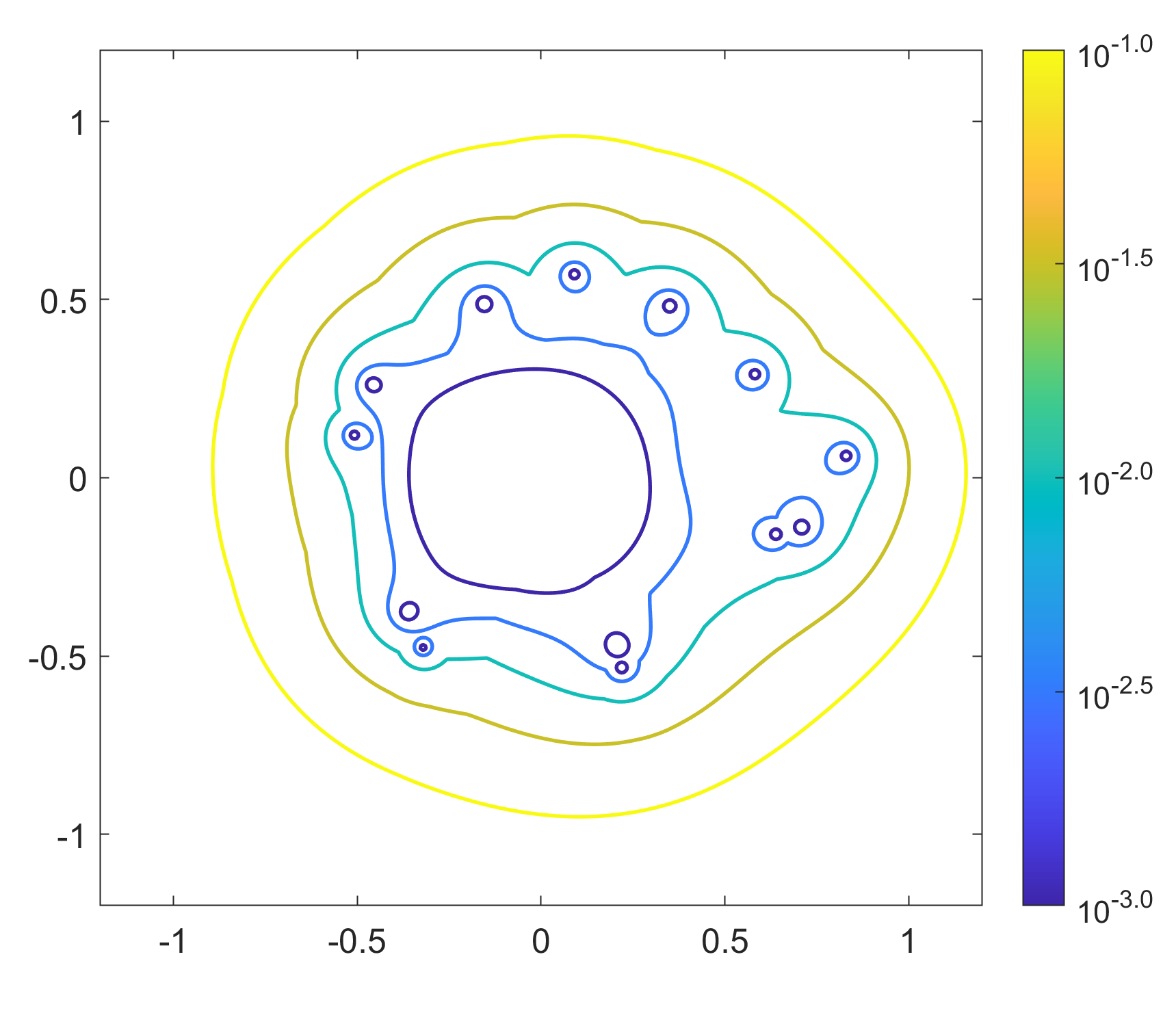
(a) $\varepsilon$-pseudospectra of $\mathcal{F}^{L}$

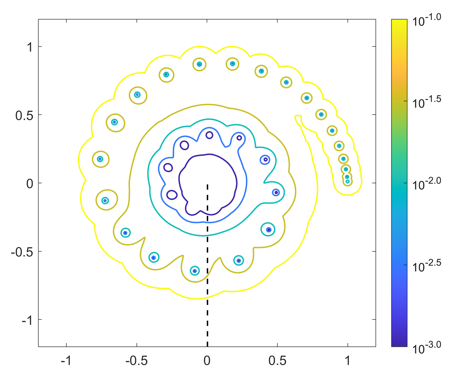
(b) $\varepsilon$-pseudospectra of $\mathcal{F}_{c}^{L}$

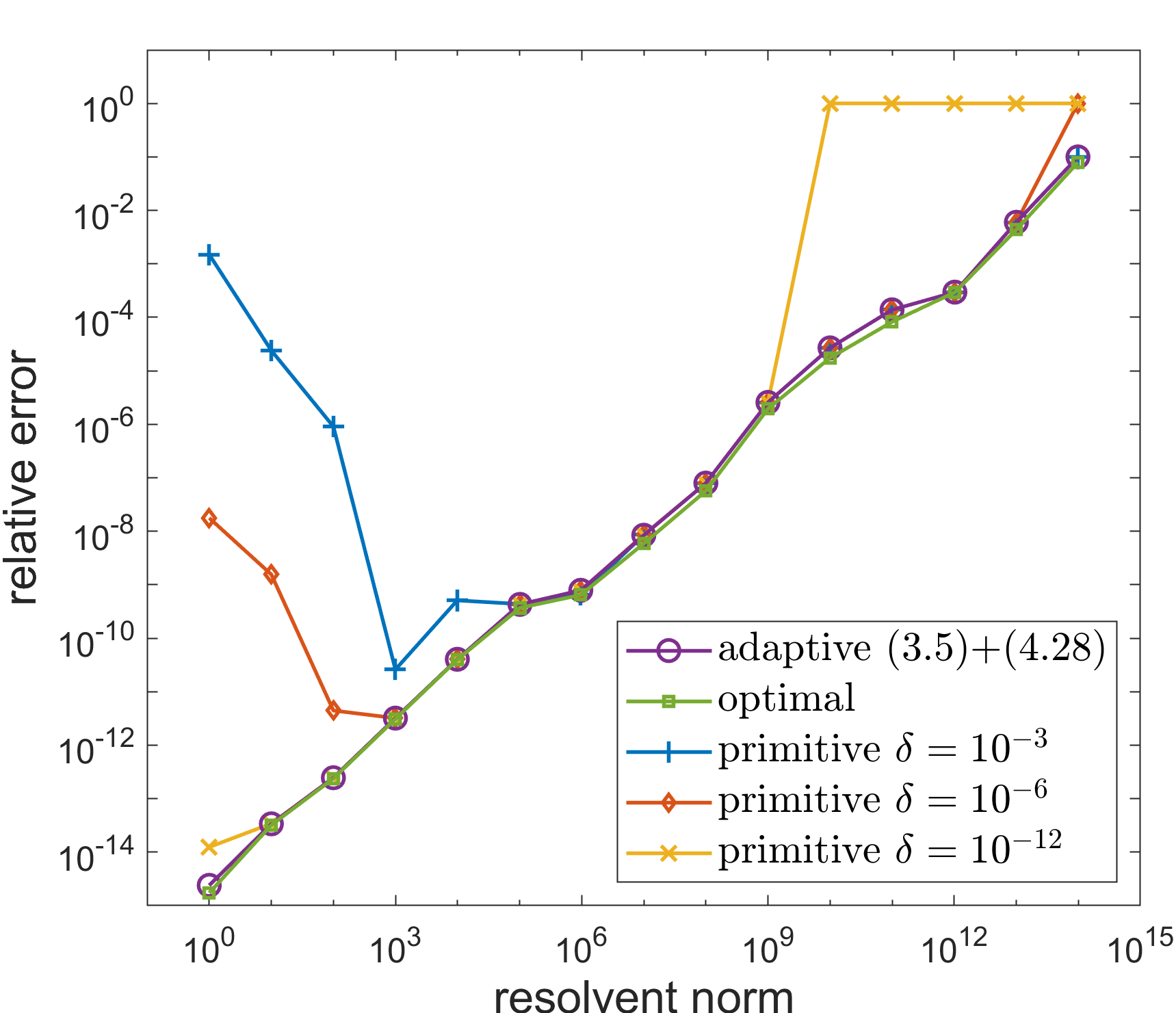
(c) relative error

Figure 1: Huygens–Fresnel operators

Our first problems are the Huygens–Fresnel operators

$$(\mathcal{F}^{L}u)(s)=\sqrt{\frac{iF}{\pi}}\int_{-1}^{1}e^{-iFM(s/M-t)^{2}}u(t)\mathrm{d}t,~{}~{}~{}(\mathcal{F}_{c}^{L}u)(s)=\sqrt{\frac{iF}{\pi}}\int_{-1}^{1}e^{-iF(s-t)^{2}}u(t)\mathrm{d}t$$

from modeling the laser problem [37, §60]. These integral operators acting on $u\in L_{2}([-1,1])$ correspond to unstable and stable resonators respectively with the former being a general Fredholm operator and the latter a Fredholm operator of convolution type. By setting the Fresnel number $F=16\pi$ and the magnification $M=2$, we use the proposed method to reproduce the second panels of Figures 60.6 and 60.2 from [37, §60], as shown in Figs. 1a and 1b. The contours at $\varepsilon=10^{-1},10^{-1.5},\dots,10^{-3}$ are a spot-on-match with the ones that Trefethen and Embree obtained using the traditional method.

Fig. 1c shows the resolvent norm versus the relative error obtained with the adaptive stopping criterion (purple) for the $15$ intersection points of the vertical dashed line at $x=0$ in Fig. 1b and the boundaries of $\varepsilon$-pseudospectra for $\varepsilon=10^{0},10^{-2},\dots,10^{-14}$ (not shown). These $15$ data roughly lie on a straight line of slope $1$, confirming the analysis at the end of Section 4.2. The smallest relative error that can be achieved is also searched at each intersection point and plotted (green) for comparison. It can be seen that the deviation, if any, is tiny to eyes showing that our adaptive stopping criterion is nearly optimal. We also include three curves obtained by replacing the adaptive stopping criterion Eqs. 15 and 37 with the primitive one in line 6 of Algorithm 1 for $\delta=10^{-3},10^{-6},10^{-12}$. With too loose a $\delta$ like $10^{-3}$ (blue), the relative error fails to decay sufficiently at $z$ where the resolvent norm is small or moderate, whereas a $\delta$ that is excessively stringent like $10^{-12}$ (yellow) results in nonconvergence for $z$ with a large resolvent norm. When $\delta=10^{-6}$ (red), both issues arise.

5.2 First derivative operator

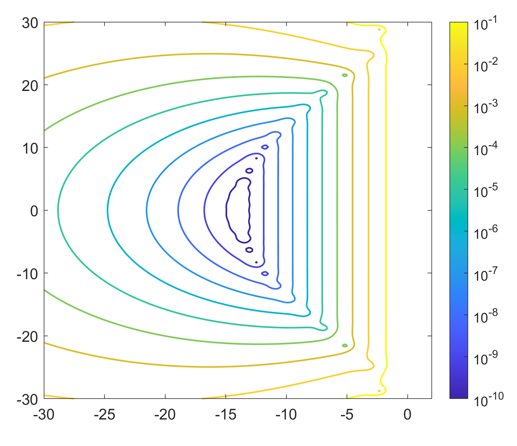
(a) traditional method

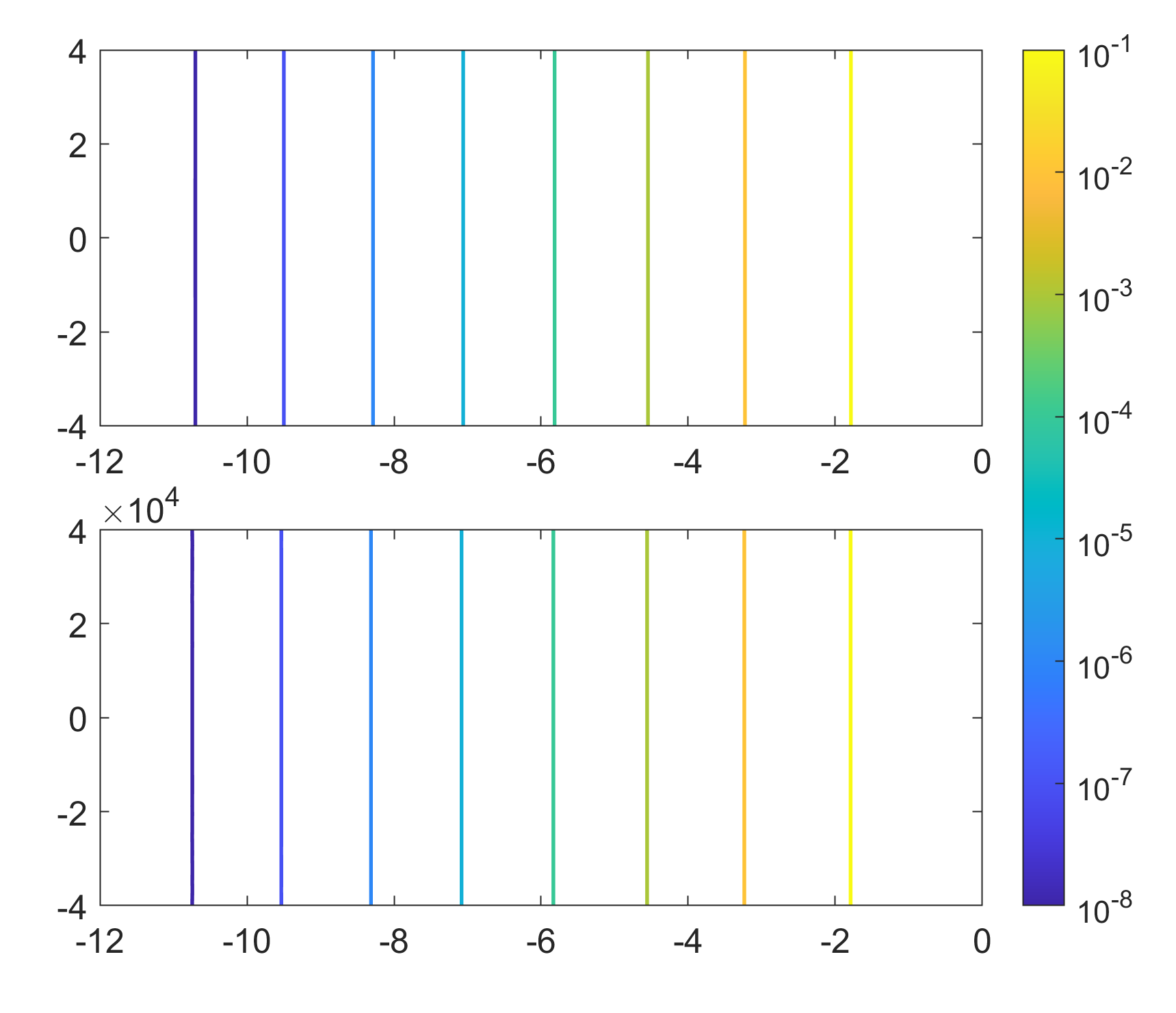
(b) proposed method

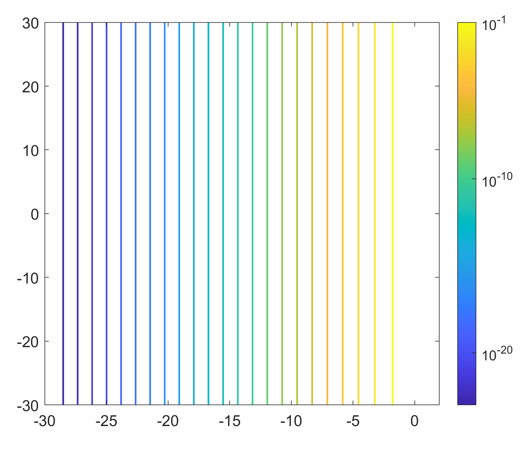
(c) extending to the left

Figure 2: $\varepsilon$-pseudospectra of the first derivative operator.

Our second example is the first derivative operator

$$\mathcal{Q}^{F}u=\frac{\mathrm{d}u}{\mathrm{d}x},$$

acting on $L^{2}([0,2])$ and subject to $u(2)=0$ [27, 35, 37]. This simple yet interesting operator features nonexistence of eigenvalues and eigenmodes, and its resolvent norm depends only on $\Re(z)$, implying that the pseudospectra contours are straight vertical lines. The pseudospectra plot obtained by the traditional method is shown in Fig. 2a. The discretize-then-solve paradigm is at least partially failed for this example, if not a fiasco—only the contours in a triangular region close to the origin resemble the true pseudospectra as vertical lines and the rest of the plot is a consequence of spectral pollution.

Whereas Figure 5.2 in [37, §5] and the upper panel of Figure 3 in [35] are obtained from cropping a plot similar to Fig. 2a, the upper panel of Fig. 2b reproduces the same plot directly using the proposed method. In fact, we can go much beyond the $y$-scale in Fig. 2b—the lower panel of Fig. 2b also displays the same level sets, obtained by the new method, but with the $y$-axis limit $10,000$ times greater.

In the upper panel of Fig. 2b, the left limit is set to $\Re(z)=-12$. We actually can push it a little further to $\Re(z)=-16.2$ (not shown) where the resolvent norm there is about $10^{12.5}$, the largest that we can compute with double precision arithmetic so that the two or three digit accuracy still allows the lines generated by the contour plotter to be straight to human eyes. Since $\left\|(z-\mathcal{Q}^{F})^{-1}\right\|=e^{2|\Re(z)|}/(2|\Re(z)|)+\mathcal{O}\left(1/|\Re(z)|\right)$ for $\Re(z)<0$, the resolvent norm grows virtually exponentially toward $-\infty$. As per the discussion at the end of Section 4.2, if we intend to calculate the resolvent norm to the left of the vertical line corresponding to $\varepsilon=10^{-12.5}$, we have to resort to higher precision arithmetics. Fig. 2c shows the pseudospectra up to $x=-30$ and is meant to be compared with Fig. 2a; the calculation is done in quadruple precision with $\epsilon_{mach}\approx 1.93\times 10^{-34}$.

5.3 Advection-diffusion operator

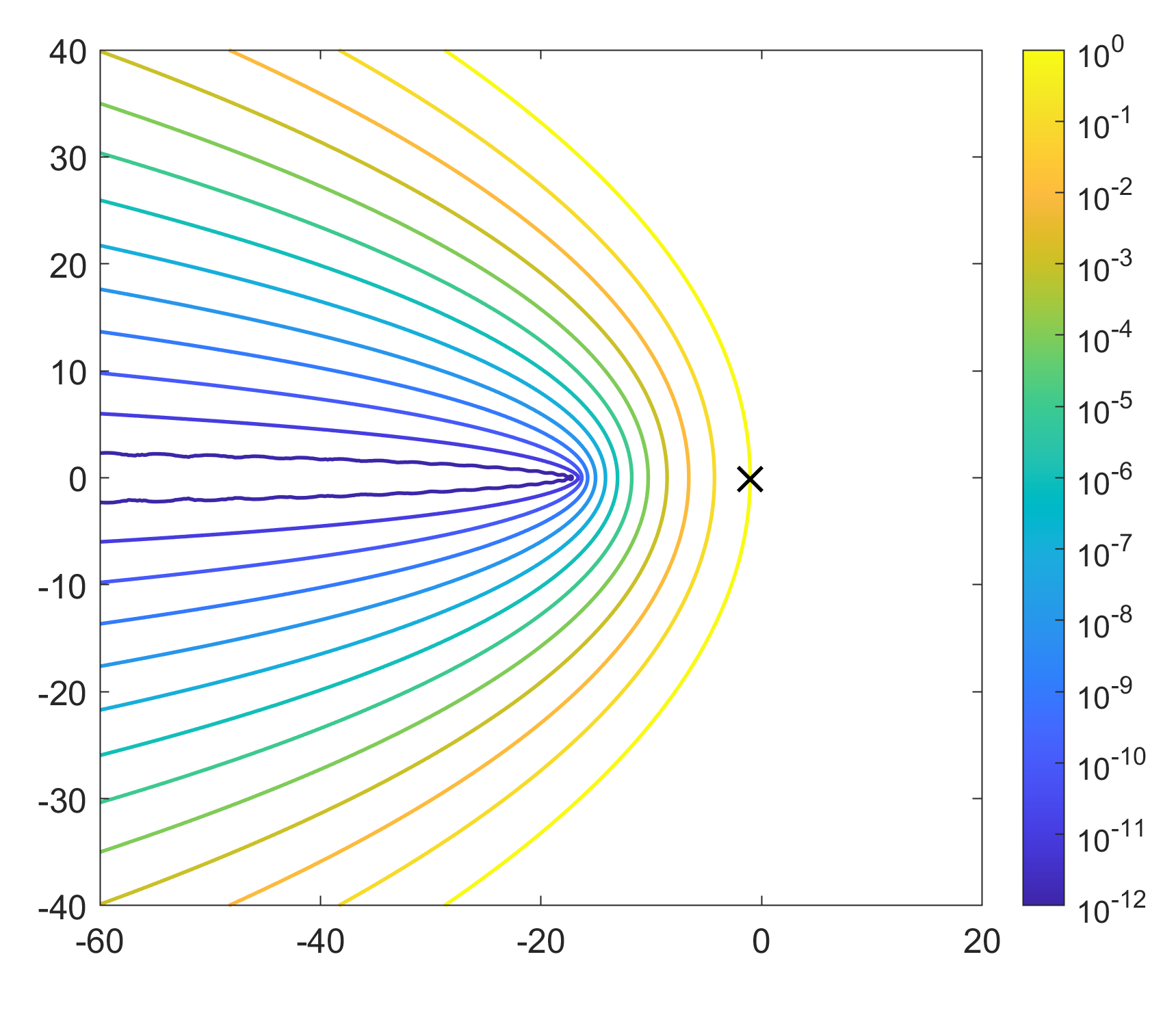
(a) $\varepsilon$-pseudospectra

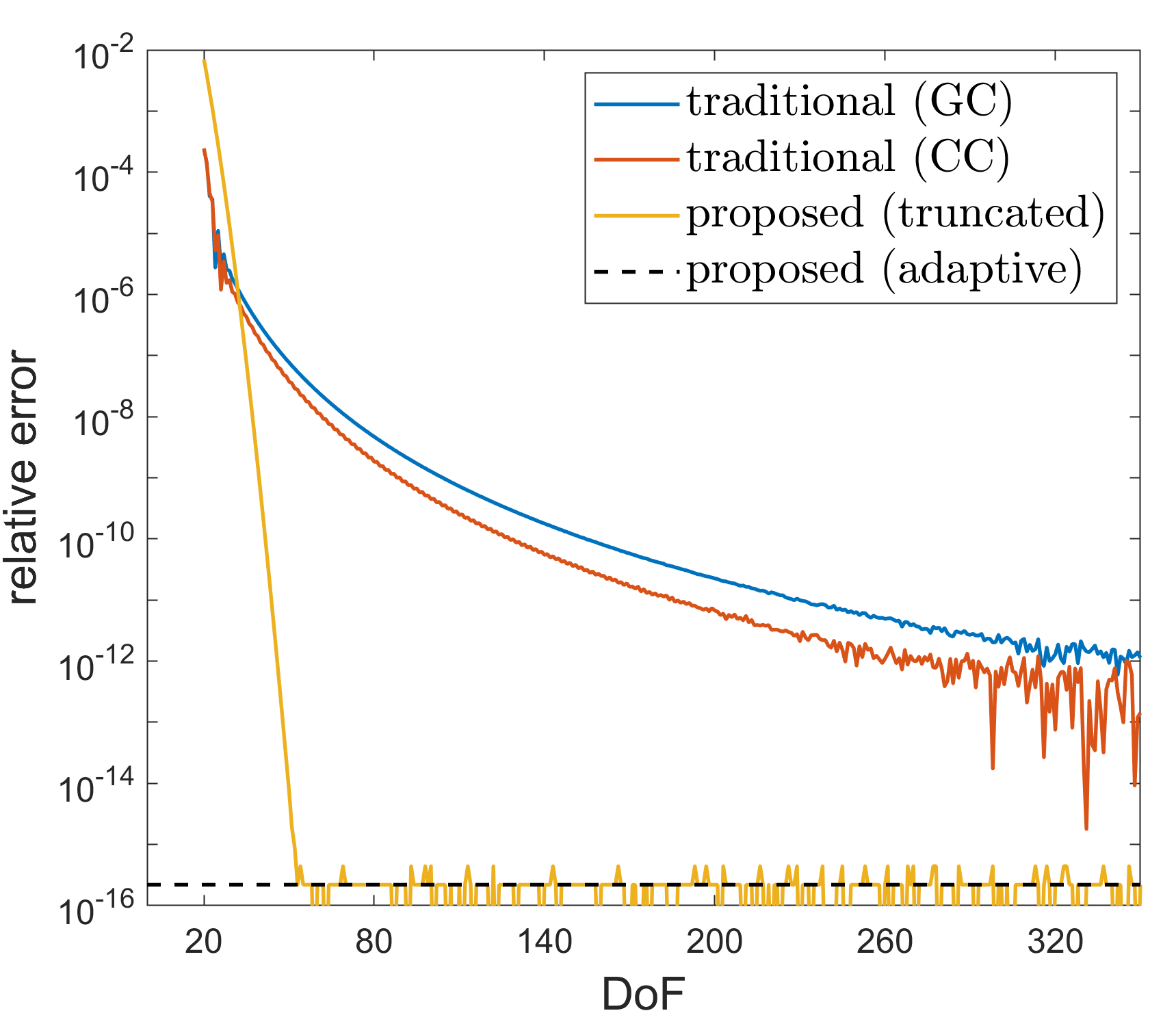
(b) spectral convergence

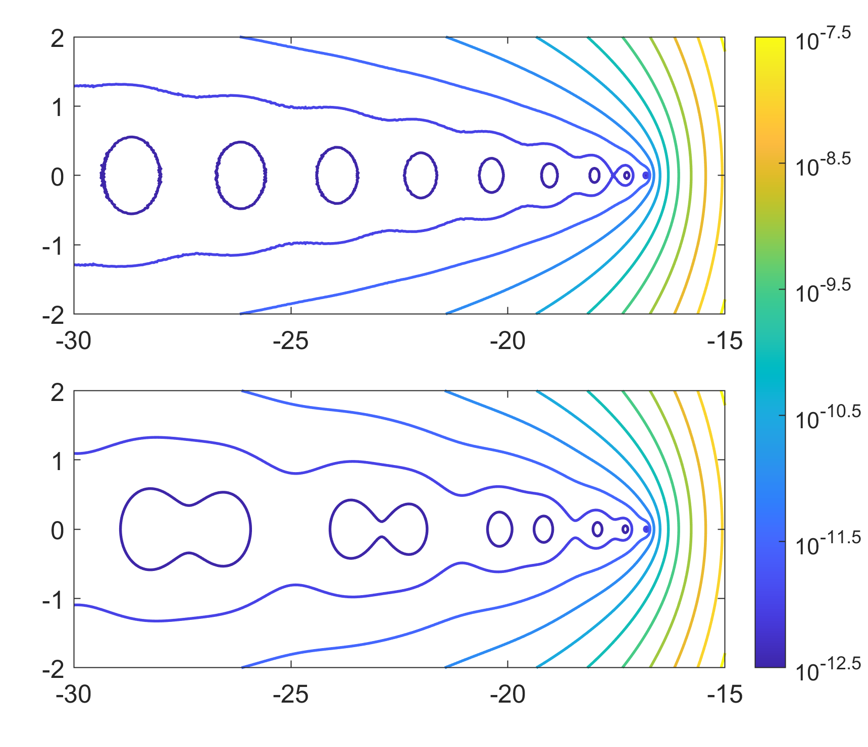
(c) close-up

Figure 3: Advection-diffusion operator

The advection-diffusion operator

$$\mathcal{Q}^{AD}=\eta\frac{\mathrm{d}^{2}}{\mathrm{d}x^{2}}+\frac{\mathrm{d}}{\mathrm{d}x}$$

acting on $L^{2}([0,1])$ and subject to the homogeneous Dirichlet boundary conditions serves in [35] and [37, §12] as an example for transient effects caused by nonnormality. The pseudospectra of $\mathcal{Q}^{AD}$ for $\eta=0.015$ is shown as Figure 12.4 in [37, §12], wheres Fig. 3a is a reproduction by the new method.

The advection-diffusion operator is also employed to demonstrate the quadrature issue related to the evaluation of the function norms [37, §43]. Trefethen and Embree suggest using a weight matrix corresponding to either Gauss–Chebyshev (GC) or Clenshaw–Curtis (CC) quadrature when Chebyshev pseudospectral method is used in a nonperiodic setting. However, they caution the loss of spectral convergence and a degeneration to algebraic convergence caused by the quadrature difficulty. This is confirmed by the blue and red curves in Fig. 3b which are the error-DoF plot of the resolvent norm at $-1.05-0.10i$ (cross in Fig. 3a). These curves are obtained using the traditional method with the GC and CC quadratures and very much resemble those given in Figure 43.5 of [37, §43] for the computed numerical abscissa. To the contrary, spectral convergence is gained by the proposed method using Legendre polynomials. This can be seen from the yellow curve which is obtained by solving Eq. 12 with a fixed $n$ throughout the Lanczos iterations and plotting the corresponding error for various $n$—the error decays exponentially to machine precision at about $n=50$ then levels off, signaling adequate resolution. Of course, we do not have to choose $n$ manually in practice. The adaptivity discussed in Section 3.1 helps us choose an optimal $n$ in each solution of Eq. 12 for complete resolutions. The resolvent norm at $-1.05-0.10i$ returned by our fully automated algorithm has an error no greater than $2.19\times 10^{-16}$, which is indicated by a dashed line in Fig. 3b for comparison with other curves.

Fig. 3c contains close-ups of Fig. 3a obtained using the proposed (upper) and the traditional (lower) methods respectively. Whereas the innermost contours in the upper panel barely hold their oval shape and start to wiggle, some of them have coalesced in the lower panel which is totally erroneous. This is because the collocation-based matrix approximation of $\mathcal{Q}^{AD}$ is ill-conditioned. It worsens the conditioning of the original problem and put the calculation at risk. Thanks to the well-conditioned ultraspherical spectral methods, the precision is made the most of with only minimal loss of digits in solving Eq. 12.

5.4 OTV and Wiener-Hopf operators

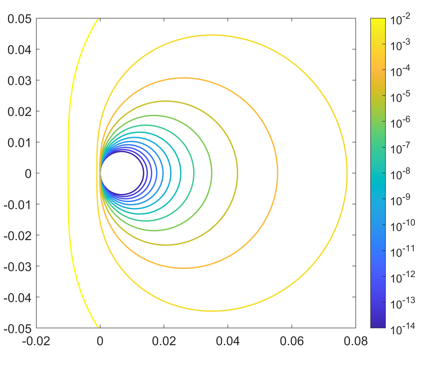
(a) $\varepsilon$-pseudospectra of OTV operator

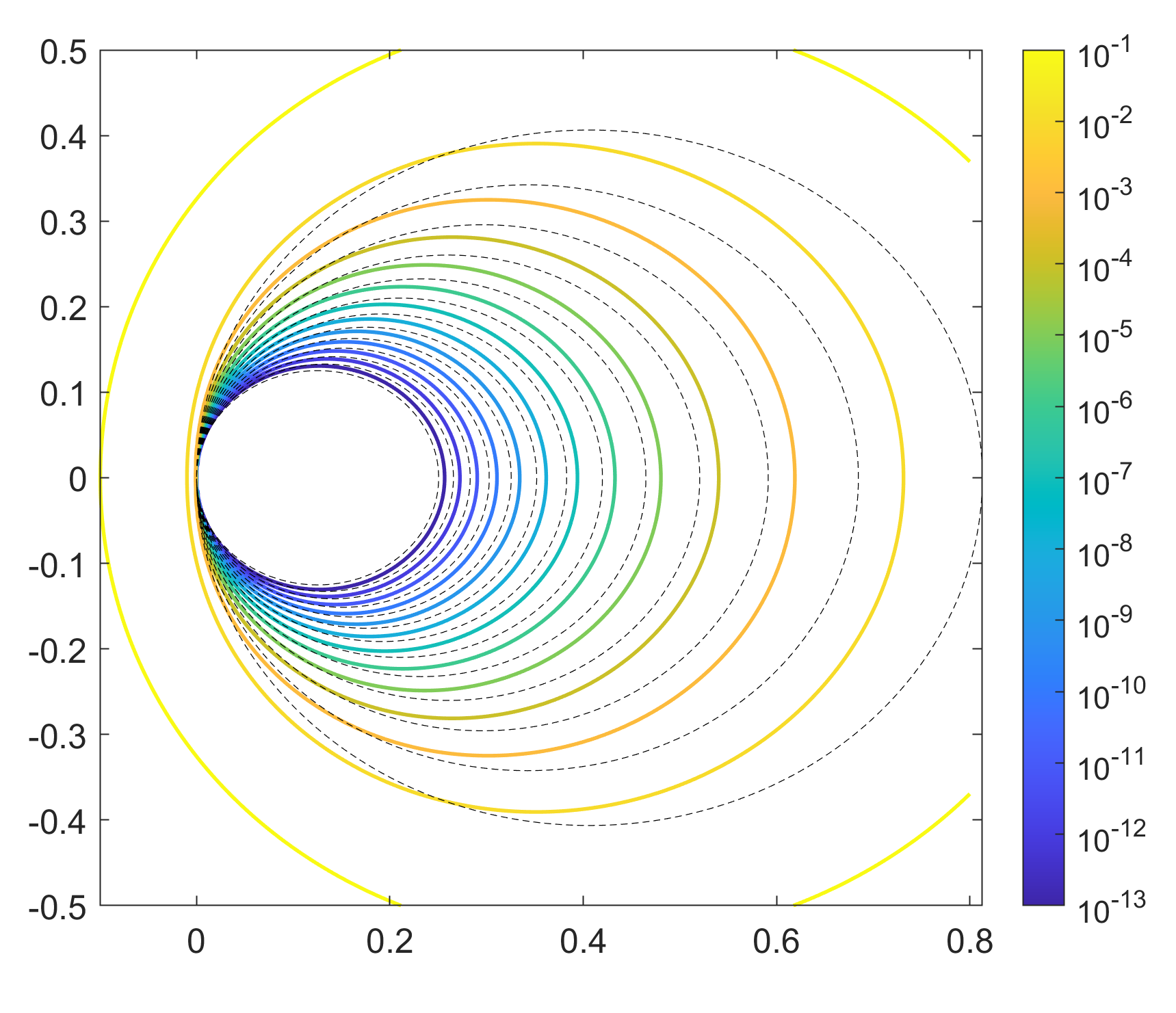
(b) $\varepsilon$-pseudospectra of Wiener-Hopf operator

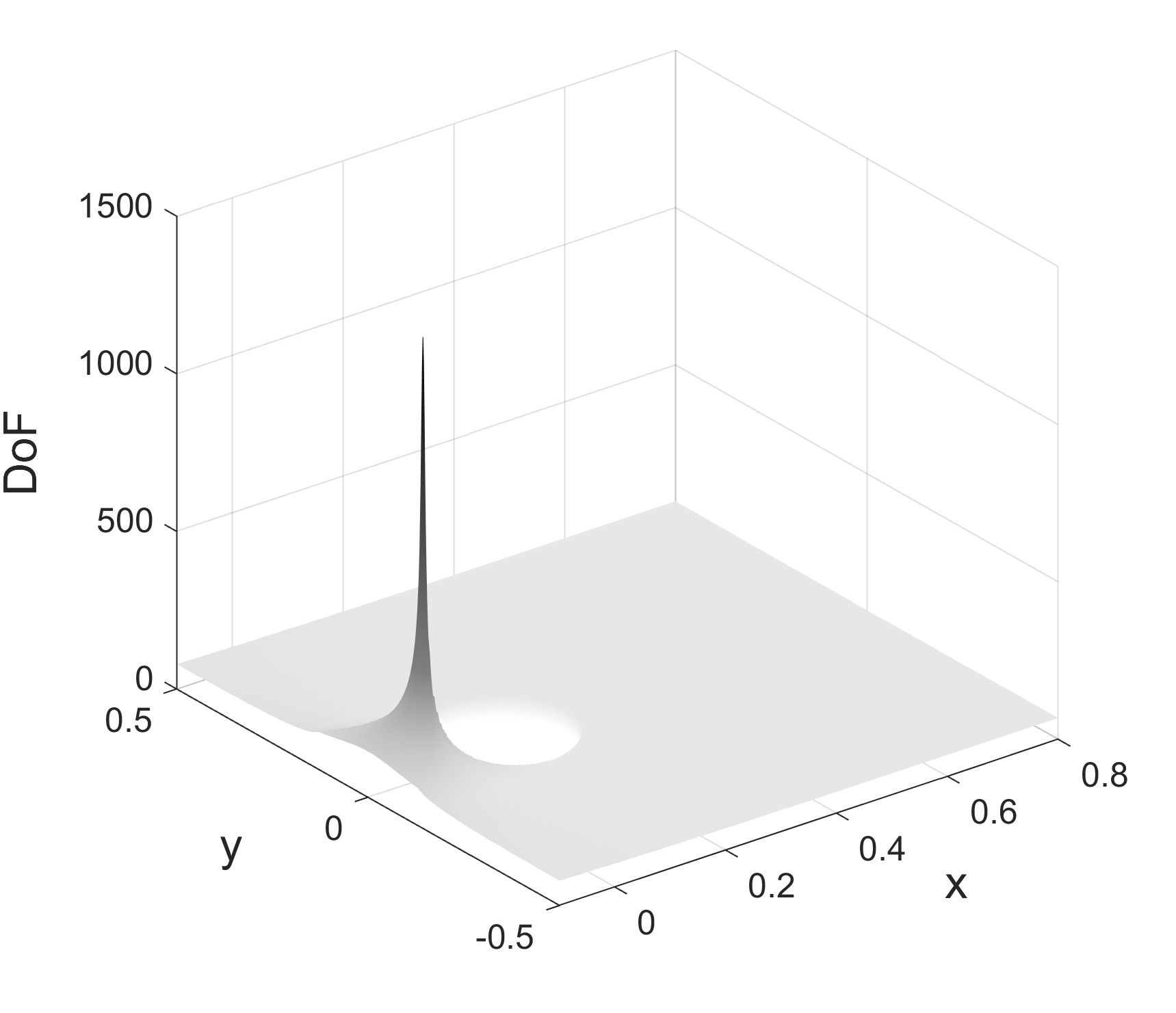
(c) pointwise DoF

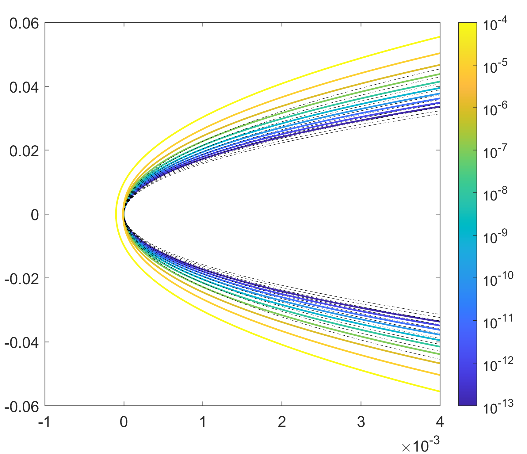
(d) adaptive DoF

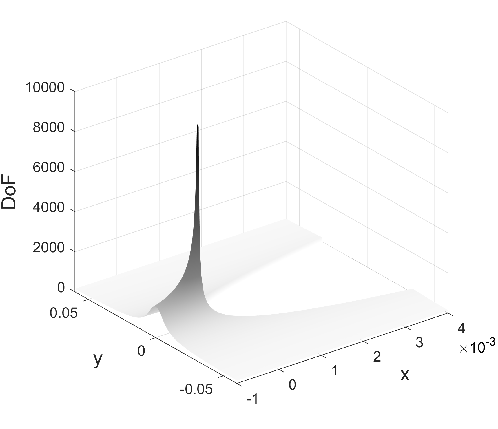
(e) pointwise DoF (close-up)

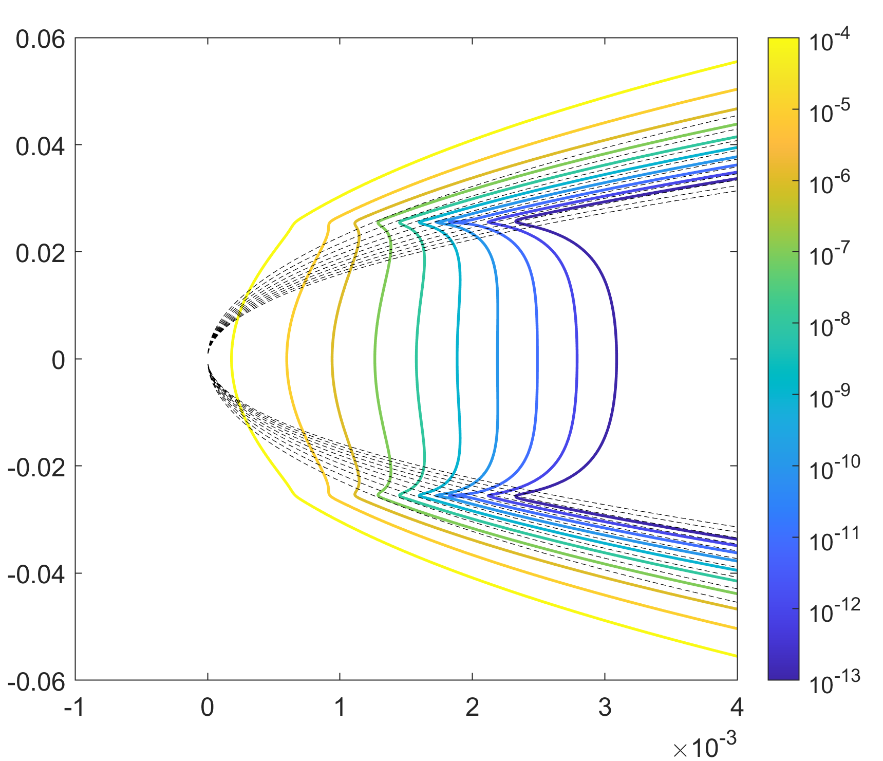
(f) $n=200$

Figure 4: OTV and Wiener-Hopf operators

Fig. 4a shows the $\varepsilon$-pseudospectra of the OTV operator [24]

$$(\mathcal{V}^{OTV}u)(s)=\int_{0}^{s}e^{-10(s-\frac{1}{3})^{2}-10(t-\frac{1}{3})^{2}}u(t)\mathrm{d}t,~{}~{}~{}~{}s\in[0,1],$$

which is computed via the approach elaborated in Section 3.1.4. Interestingly, we have not found any $\varepsilon$-pseudospectra plot of a general Volterra operator in the literature. This $\varepsilon$-pseudospectra plot resembles very much that of the Wiener-Hopf operator that is well-studied. The Wiener-Hopf operator

$$(\mathcal{V}^{WH}_{c}u)(s)=\int_{s}^{d}e^{s-t}u(t)\mathrm{d}t,~{}~{}~{}~{}s\in[0,10]$$

is a Volterra operator of convolution type. Previous study on its nonnormality and pseudospectra includes, e.g., [27, 35].

We show in Fig. 4b the pseudospectra of the Wiener-Hopf operator $\mathcal{V}_{c}$ for $d=10$ by the boundaries of $\varepsilon$-pseudospectra for $\varepsilon=10^{-1},10^{-2},\dots,10^{-13}$. These boundaries are in good agreement with their respective lower bounds (dashed curves) [27]. Specifically, the resolvent norm is calculated on a grid of $600\times 600$ points before the results are sent to the contour plotter. For each grid point the largest $n$ used throughout the Lanczos process is shown in Fig. 4c. It can be seen that $n$ grows as $z$ gets closer to the origin. At $-8.35\times 10^{-4}\pm 8.35\times 10^{-4}i$, the closest grid points to the origin, the computed solution to Eq. 12 is approximated by a Legendre series of degree $1402$, the highest among all the grid points.

Fig. 4d is a close-up near the origin with the resolvent norm computed on a $800\times 800$ grid. As shown in Fig. 4e, $n=9935$ for a complete resolution at $1.25\times 10^{-6}\pm 7.51\times 10^{-5}i$, the grid points nearest to the origin. Thanks to the adaptivity, the determination of $n$ is fully automated and sufficient resolution is guaranteed. In principle, the proposed method can compute the resolvent norm at a point arbitrarily close to the spectra, provided that sufficiently powerful hardware is available.

For comparison, Fig. 4f shows the boundaries of $\varepsilon$-pseudospectra obtained with $n=200$ throughout the entire grid. This “finite section” type implementation produces contours that exhibit conspicuous violation to the lower bounds for all the $\varepsilon$ considered, highlighting the importance of the adaptivity in DoF $n$.

5.5 Orr-Sommerfeld

(a) $L^{2}$ norm

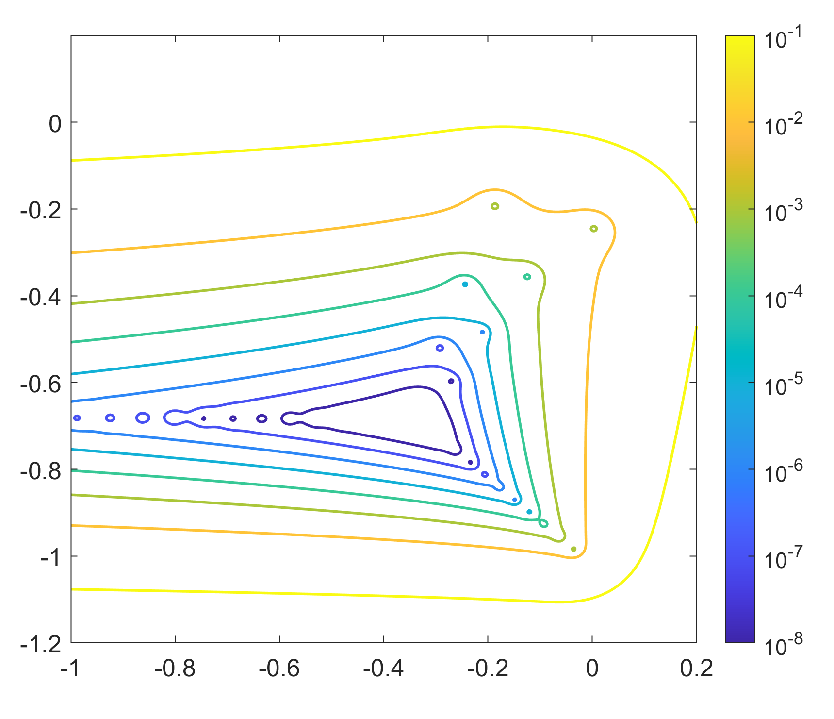
(b) energy norm

Figure 5: $\varepsilon$-pseudospectra of the Orr-Sommerfeld operator.

We close this section with the Orr-Sommerfeld operator for which pseudospectra plays a pivotal role in analyzing the temporal stability of fluid flows, as detailed in [28] and [37, §22]. In the standard form of Eq. 9, the differential expressions of $\mathcal{A}$ and $\mathcal{B}$ read

$$\tau_{\mathcal{A}}=-\frac{1}{R}\left(\frac{\mathrm{d}^{2}}{\mathrm{d}x^{2}}-\alpha^{2}\right)^{2}+i\alpha(1-x^{2})\left(\frac{\mathrm{d}^{2}}{\mathrm{d}x^{2}}+\alpha^{2}\right)+2i\alpha,~{}~{}~{}\tau_{\mathcal{B}}=-\frac{\mathrm{d}^{2}}{\mathrm{d}x^{2}}+\alpha^{2}$$

with $\mathcal{A}$ attached with $u(\pm 1)=0$ and $u^{\prime}(\pm 1)=0$ and $\mathcal{B}$ with $u(\pm 1)=0$.

Fig. 5a displays the $2$-norm pseudospectra for $R=5772$ and $\alpha=1.02$ which is obtained following the details given in Section 3.1.6. If it is the pseudospectra in the energy norm [28] defined by

$$\langle\phi,\psi\rangle_{E}=\langle\mathcal{B}\phi,\psi\rangle$$

that we look at, we should note that $\mathcal{R}^{*}(z)$ is different from Eq. 10a as the latter is obtained via the Euclidean inner product. Suppose that $\phi,\psi\in\mathcal{D}(\mathcal{B})$. Reworking out as we do in Eq. 11 and noting $\mathcal{B}=\mathcal{B}^{*}$ for this particular example, we have

$$\langle\mathcal{R}(z)\phi,\psi\rangle_{E}=\langle\mathcal{B}\phi,(z^{*}\mathcal{B}-\mathcal{A}^{*})^{-1}\mathcal{B}\psi\rangle=\langle\phi,(z^{*}\mathcal{B}-\mathcal{A}^{*})^{-1}\mathcal{B}\phi\rangle_{E}.$$

Thus, $\mathcal{R}^{*}(z)=(z^{*}\mathcal{B}-\mathcal{A}^{*})^{-1}\mathcal{B}$. Since $\mathcal{R}(z)$ is not changed with the norm, Eq. 10b still holds and we take exactly the procedure following Eq. 14 to apply $\mathcal{R}(z)$. Then applying $\mathcal{R}^{*}(z)$, i.e., $w=(z^{*}\mathcal{B}-\mathcal{A}^{*})^{-1}\mathcal{B}v$, is done by solving $(z^{*}\mathcal{B}-\mathcal{A}^{*})w=\mathcal{B}v$. Fig. 5b is a reproduction of Figure 2 in [28], showing the $\varepsilon$-pseudospectra in energy norm for $\varepsilon=10^{-1},10^{-2},\dots,10^{-8}$.

6 Extensions

In this section, we discuss a few extensions of the proposed method, which, along with those dealt with in the previous sections, cover a great portion of the pseudospectra problems that one may come across in practice.

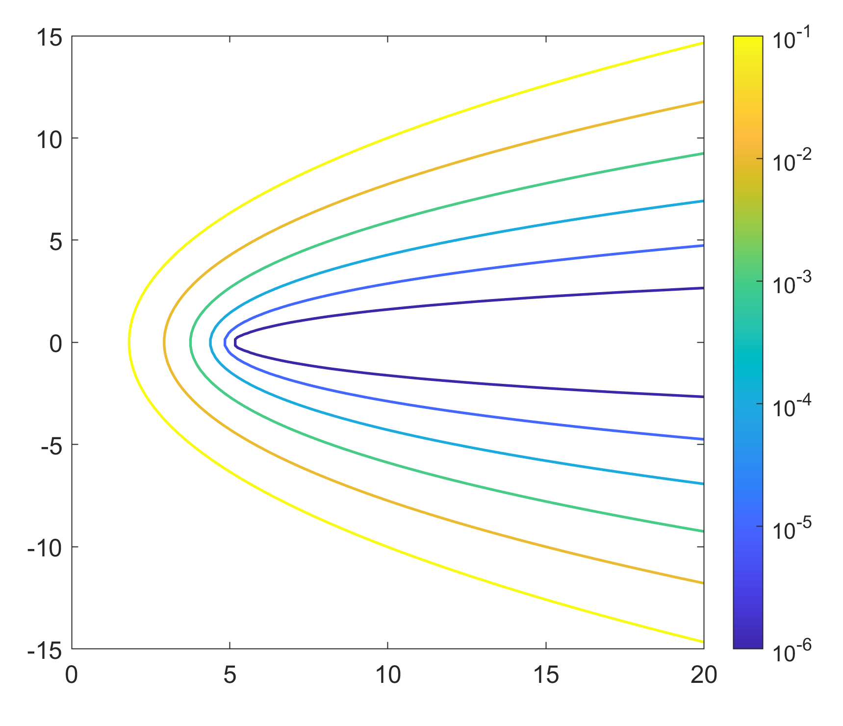
(a) 2D advection-diffusion operator

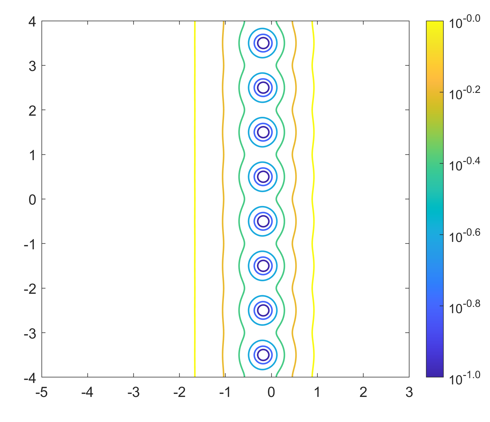
(b) wave operator

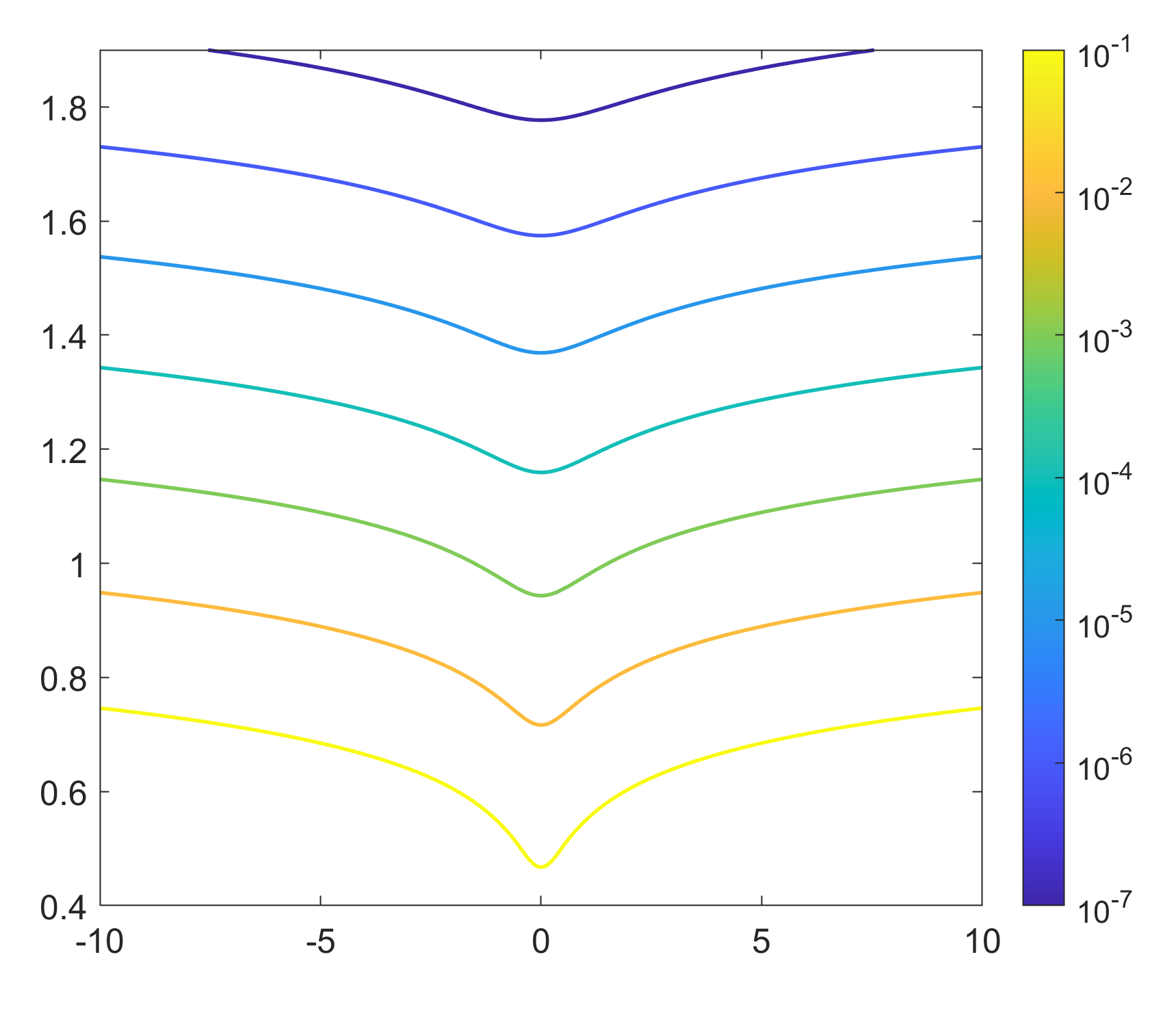
(c) acoustic wave problem

Figure 6: $\varepsilon$-pseudospectra of multivariate operator, block operator, and nonlinear eigenvalue problem examples.

6.1 Multivariate operators

The existing strategies for handling an operator $\mathcal{L}$ acting in multiple space dimensions include decoupling the pseudospectra problem into problems of lower dimension [37, §43] and representing $\mathcal{L}$ as an operator acting on $\ell^{2}(\mathbb{N})$ [6, 8]. On the other hand, the framework presented in this paper applies perfectly to an operator in multiple dimensions, provided that its resolvent is compact or compact-plus-scalar. We now take as an example the Dirichlet operator [13, §XIV.6], noting that most of the elliptic operators fall into this category.

Given a bounded open set $\Omega$ in $\mathbb{R}^{d}$ and a partial differential expression

$$\tau_{e}=\sum_{i,j=1}^{d}a_{ij}(\mathbf{x})\frac{\partial}{\partial x_{i}}\frac{\partial}{\partial x_{j}}+\sum_{i=1}^{d}b_{i}(\mathbf{x})\frac{\partial}{\partial x_{i}}+c(\mathbf{x})u,$$

where each $a_{ij}$, $b_{i}$, and $c$ are in $C^{\infty}(\bar{\Omega})$ and $\bar{\Omega}$ is the closure of $\Omega$. The Dirichlet operator $\mathcal{P}:L^{2}(\Omega)\rightarrow L^{2}(\Omega)$ is defined as $\mathcal{P}u=\tau_{e}u$ with $\mathcal{D}(\mathcal{P})=H_{0}^{1}(\Omega)\cap H^{2}(\Omega)$. If $\mathcal{P}$ is uniformly elliptic, $\mathcal{R}(z)=(z\mathcal{I}-\mathcal{P})^{-1}$ is compact for $z\in\mathbb{C}\backslash\sigma(\mathcal{P})$ [13, §XIV.6].

In implementing Algorithms 2 and 3, we need to adapt at only one place—Eq. 12 is to be solved by an elliptic PDE solver, for example, the multivariate ultraspherical spectral method [31, 33]. Fig. 6a shows the pseudospectra of the 2D advection-diffusion operator [17]

$$\mathcal{P}^{AD}u=\eta\Delta u+\mathbf{V}\cdot\nabla u$$

in $\Omega=[0,1]\times[0,1]$ with $\eta=0.05$ and $\mathbf{V}=[0,1]^{T}$.

6.2 Block operators

It is not uncommon to consider the pseudospectra of block operators that act on Cartesian product of function spaces. Such an operator may come from reducing a high-order problem to a system of low-order ones. For example, Trefethen and Driscoll in [10, 35] investigated the wave operator

$$\mathcal{Q}^{B}=\begin{pmatrix}0&\mathrm{d}/\mathrm{d}x\\ \mathrm{d}/\mathrm{d}x&0\end{pmatrix}$$

with $\mathcal{D}(\mathcal{Q}^{B})=\left\{(u,v)\in L^{2}([0,\pi])\times L^{2}([0,\pi])\mid v(0)=0,\ u(\pi)+\eta v(\pi)=0\right\}$ and $\eta=1/2$. The compactness of $(z\mathcal{I}-\mathcal{Q}^{B})^{-1}$ can be established following the proof in [13, §XI.1]. Fig. 6b displays the pseudospectra of $\mathcal{L}$ obtained using the proposed method. This replicates Figure 3 in [10], which was originally produced from a finite-dimensional discretization of $\mathcal{Q}^{B}$ using the finite difference method. In solving Eq. 12 with the ultraspherical spectral method, each $\mathrm{d}/\mathrm{d}x$ corresponds to an infinite-dimensional banded matrix, thus representing $\mathcal{Q}^{B}$ by a $2\times 2$ block matrix with the $(1,2)$ and $(2,1)$ blocks being infinitely banded. Applying a simple reordering and prepending the boundary conditions give an infinite-dimensional almost-banded system, which we solve again by adaptive QR.

6.3 Nonlinear eigenvalue problems

In [9], Colbrook and Townsend show that the $\varepsilon$-pseudospectrum of NEP $\mathcal{N}(\lambda)=0$ can be defined as

$$\sigma_{\varepsilon}(\mathcal{N})=\left\{z\in\mathbb{C}:\|\mathcal{N}(z)^{-1}\|>\varepsilon^{-1}\right\}.$$

Since $z$ is always given as known, the computation of the resolvent norm of $\mathcal{N}$ is a perfectly linear problem and $\mathcal{N}(z)$ is therefore a closed linear operator. When $\mathcal{N}(z)^{-1}$ is compact or compact-plus-scalar, its resolvent norm can be computed with the proposed method. As an example, we consider the acoustic wave problem in [2]

$$\mathcal{N}(z)u=\frac{\mathrm{d}^{2}u}{\mathrm{d}x^{2}}+4\pi^{2}z^{2}u,$$

subject to $u(0)=0$ and $\eta u^{\prime}(1)+2\pi izu(1)=0$. This serves as another example of an empty spectrum. Fig. 6c shows the pseudospectra of $\mathcal{N}(z)$ for $\eta=1$.

6.4 Other inner products

In most cases, we work in a Hilbert space that is equipped with the Euclidean inner product and the $L^{2}$ norm. If it is the pseudospectra in other norms that is of interest, Algorithm 3 remains largely unchanged only except that $\alpha_{k}$ and $\beta_{k}$ are to be evaluated with the right inner product and the adjoint operator should be re-determined accordingly. This is exactly how we deal with the energy norm in Section 5.5.

Particularly, for the weighted $L^{2}$ inner product

$$\langle u,v\rangle_{w}=\int_{a}^{b}w(x)u^{*}(x)v(x)dx$$

which is associated with the orthonormal polynomial $\{\varphi_{k}(x)\}_{k=0}^{\infty}$, $\langle u,v\rangle_{w}$ and the weighted $L^{2}$-norm correspond precisely to the dot product and the $l^{2}$-norm of the coefficient vectors in $\{\varphi_{k}(x)\}_{k=0}^{\infty}$, respectively. In addition, if the matrix representation of a bounded operator $\mathcal{L}$ under $\{\varphi_{k}(x)\}_{k=0}^{\infty}$ is available, it can be shown that the matrix representation of $\mathcal{L}^{*}$ is simply the adjoint of that of $\mathcal{L}$.

7 Conclusion

We have proposed a continuous framework for computing the pseudospectra of linear operators. The new method features adaptivity in both the stopping criterion for the operator Lanczos iteration and the DoF for resolved solutions to the inverse resolvent equations, achieving near-optimal accuracy. The spectral pollution and invisibility are eradicated and the convergence in terms of DoF is spectral. The adoption of the well-conditioned spectral methods prevents any deterioration in the conditioning of the problem.

References

- [1] J. L. Aurentz and L. N. Trefethen, Chopping a Chebyshev series, ACM Transactions on Mathematical Software, 43 (2017), pp. 1–21.
- [2] T. Betcke, N. J. Higham, V. Mehrmann, C. Schröder, and F. Tisseur, NLEVP: A collection of nonlinear eigenvalue problems, ACM Transactions on Mathematical Software, 39 (2013), pp. 1–28.
- [3] S. Chandrasekaran and M. Gu, Fast and stable algorithms for banded plus semiseparable systems of linear equations, SIAM Journal on Matrix Analysis and Applications, 25 (2003), pp. 373–384.
- [4] L. Cheng and K. Xu, Understanding the ultraspherical spectral method, In preparation, (2024).
- [5] M. J. Colbrook, Computing semigroups with error control, SIAM Journal on Numerical Analysis, 60 (2022), pp. 396–422.
- [6] M. J. Colbrook and A. C. Hansen, The foundations of spectral computations via the solvability complexity index hierarchy, Journal of the European Mathematical Society, 25 (2022), pp. 4639–4718.
- [7] M. J. Colbrook, A. Horning, and A. Townsend, Computing spectral measures of self-adjoint operators, SIAM Review, 63 (2021), pp. 489–524.
- [8] M. J. Colbrook, B. Roman, and A. C. Hansen, How to compute spectra with error control, Physical Review Letters, 122 (2019), p. 250201.
- [9] M. J. Colbrook and A. Townsend, Avoiding discretization issues for nonlinear eigenvalue problems, arXiv preprint arXiv:2305.01691, (2023).
- [10] T. A. Driscoll and L. N. Trefethen, Pseudospectra for the wave equation with an absorbing boundary, Journal of Computational and Applied Mathematics, 69 (1996), pp. 125–142.
- [11] M. A. Gilles and A. Townsend, Continuous analogues of Krylov subspace methods for differential operators, SIAM Journal on Numerical Analysis, 57 (2019), pp. 899–924.
- [12] I. Gohberg, S. Goldberg, and M. A. Kaashoek, Basic Classes of Linear Operators, Birkhäuser, 2012.
- [13] I. Gohberg, S. Goldberg, and M. A. Kaashoek, Classes of Linear Operators, Birkhäuser, 2013.
- [14] N. Hale and A. Townsend, An algorithm for the convolution of Legendre series, SIAM Journal on Scientific Computing, 36 (2014), pp. A1207–A1220.
- [15] N. Hale and A. Townsend, A fast FFT-based discrete Legendre transform, IMA Journal of Numerical Analysis, 36 (2016), pp. 1670–1684.
- [16] A. C. Hansen, Infinite-dimensional numerical linear algebra: theory and applications, Proceedings of the Royal Society A: Mathematical, Physical and Engineering Sciences, 466 (2010), pp. 3539–3559.
- [17] L. Hemmingsson, A semi-circulant preconditioner for the convection-diffusion equation, Numerische Mathematik, 81 (1998), pp. 211–248.
- [18] N. J. Higham, Accuracy and Stability of Numerical Alorithms, vol. 61, SIAM, 1998.
- [19] A. Horning and A. Townsend, FEAST for differential eigenvalue problems, SIAM Journal on Numerical Analysis, 58 (2020), pp. 1239–1262.
- [20] R. B. Lehoucq, D. C. Sorensen, and C. Yang, ARPACK users’ guide: solution of large-scale eigenvalue problems with implicitly restarted Arnoldi methods, SIAM, 1998.
- [21] X. Liu, K. Deng, and K. Xu, Spectral approximation of Fredholm convolution operators, submitted, (2024).
- [22] S. Lui, Computation of pseudospectra by continuation, SIAM Journal on Scientific Computing, 18 (1997), pp. 565–573.
- [23] S. Olver and A. Townsend, A fast and well-conditioned spectral method, SIAM Review, 55 (2013), pp. 462–489.
- [24] S. Olver, A. Townsend, and G. Vasil, A sparse spectral method on triangles, SIAM Journal on Scientific Computing, 41 (2019), pp. A3728–A3756.
- [25] C. C. Paige, Error analysis of the Lanczos algorithm for tridiagonalizing a symmetric matrix, IMA Journal of Applied Mathematics, 18 (1976), pp. 341–349.
- [26] C. C. Paige, Accuracy and effectiveness of the Lanczos algorithm for the symmetric eigenproblem, Linear algebra and its applications, 34 (1980), pp. 235–258.
- [27] S. C. Reddy, Pseudospectra of Wiener-Hopf integral operators and constant-coefficient differential operators, Journal of Integral Equations and Applications, (1993), pp. 369–403.
- [28] S. C. Reddy, P. J. Schmid, and D. S. Henningson, Pseudospectra of the Orr-Sommerfeld operator, SIAM Journal on Applied Mathematics, 53 (1993), pp. 15–47.
- [29] Y. Saad, On the rates of convergence of the Lanczos and the block-Lanczos methods, SIAM Journal on Numerical Analysis, 17 (1980), pp. 687–706.
- [30] F. Smithies, Integral Equations, no. 49, CUP Archive, 1958.
- [31] C. Strössner and D. Kressner, Fast global spectral methods for three-dimensional partial differential equations, IMA Journal of Numerical Analysis, 43 (2023), pp. 1519–1542.
- [32] G. Szegő, Orthogonal Polynomials, vol. 23, American Mathematical Society, 1939.
- [33] A. Townsend and S. Olver, The automatic solution of partial differential equations using a global spectral method, Journal of Computational Physics, 299 (2015), pp. 106–123.
- [34] A. Townsend and L. N. Trefethen, An extension of Chebfun to two dimensions, SIAM Journal on Scientific Computing, 35 (2013), pp. C495–C518.
- [35] L. N. Trefethen, Pseudospectra of linear operators, SIAM Review, 39 (1997), pp. 383–406.
- [36] L. N. Trefethen, Computation of pseudospectra, Acta Numerica, 8 (1999), pp. 247–295.
- [37] L. N. Trefethen and M. Embree, Spectra and Pseudospectra: The Behaviour of Non-normal Matrices and Operators, Princeton University Press, 2005.
- [38] K. Xu and A. F. Loureiro, Spectral approximation of convolution operators, SIAM Journal on Scientific Computing, 40 (2018), pp. A2336–A2355.