Understanding the effects of spacecraft trajectories through solar coronal mass ejection flux ropes using 3DCOREweb

Abstract

This study investigates the impact of spacecraft positioning and trajectory on in situ signatures of coronal mass ejections (CMEs). Employing the 3DCORE model, a 3D flux rope model that can generate in situ profiles for any given point in space and time, we conduct forward modeling to analyze such signatures for various latitudinal and longitudinal positions, with respect to the flux rope apex, at 0.8 au. Using this approach, we explore the appearance of the resulting in situ profiles for different flux rope types, with different handedness and inclination angles, for both high and low twist CMEs. Our findings reveal that even high twist CMEs exhibit distinct differences in signatures between apex hits and flank encounters, with the latter displaying stretched-out profiles with reduced rotation. Notably, constant, non-rotating in situ signatures are only observed for flank encounters of low twist CMEs, suggesting implications for the magnetic field structure within CME legs. Additionally, our study confirms the unambiguous appearance of different flux rope types in in situ signatures, contributing to the broader understanding and interpretation of observational data. Given the model assumptions, this may refute trajectory effects to be the cause for mismatching flux rope types as identified in solar signatures. While acknowledging limitations inherent in our model, such as the assumption of constant twist and non-deformable torus-like shape, we still draw relevant conclusions within the context of global magnetic field structures of CMEs and the potential for distinguishing flux rope types based on in situ observations.

1 Introduction

A major unsolved problem in space weather forecasting is the correct prediction of the time series of the solar wind magnetic field vector in near-Earth space. In particular, spacecraft have observed structures in situ in the solar wind inside interplanetary coronal mass ejections (ICMEs), which lead to the strongest excursions in the total magnetic field. ICMEs typically comprise a shock, sheath and magnetic ejecta, where the field vector smoothly rotates up to 180^∘(Zurbuchen & Richardson, 2006). This is usually interpreted as the observational signature of a spacecraft passing through a large scale magnetic flux rope within the magnetic ejecta (Burlaga et al., 1981; Marubashi, 1986; Burlaga, 1988), in which helical magnetic field lines are wound around a central axis, as described by the Lundquist (1950) or Gold & Hoyle (1960) solutions of the basic equations of magnetohydrodynamics (MHD). This picture has been generally accepted as the main concept capable of reconstructing the global structure of CMEs, and towards predicting their in situ magnetic field structure for space weather forecasting. Many different models have been developed which are based on the flux rope hypothesis (e.g. Lepping et al., 1990; Hidalgo & Nieves-Chinchilla, 2012; Isavnin, 2016; Möstl et al., 2018; Rouillard et al., 2020; Nieves-Chinchilla et al., 2020). However, other interpretations have been put forward as well, including spheromaks known as possible MHD solutions (Farrugia et al., 1995; Vandas & Romashets, 2017) or a different kind of rotating magnetic field that gives similarly rotating signatures emerging from simulations of erupting flux ropes (Al-Haddad et al., 2013, 2019).

Following Bothmer & Schwenn (1998) and Mulligan et al. (1998), there exists a comprehensive classification scheme for flux ropes, categorizing them into eight distinct types based on their chirality and orientation in space. This arises from a flux rope being characterized by both the poloidal field wrapping around, and the axial field running parallel to the central axis. Low inclination flux ropes have their central axis nearly parallel to the ecliptic plane, which leads to a change of sign in the normal magnetic field component $B_{n}$ upon crossing. Depending on their handedness and orientation of the central axis, they can be classified as one of the following: left-handed: North-West-South (NWS), South-East-North (SEN); right-handed: North-East-South (NES), South-West-North (SWN). Flux ropes with their axis nearly perpendicular to the ecliptic plane experience a sign change in the tangential component $B_{t}$ and are termed high inclination flux ropes. The four different types are: left-handed: East-North-West (ENW), West-South-East (WSE); right-handed: East-South-West (ESW), West-North-East (WNE). A graphical representation of the flux rope types is shown in Figure 1.

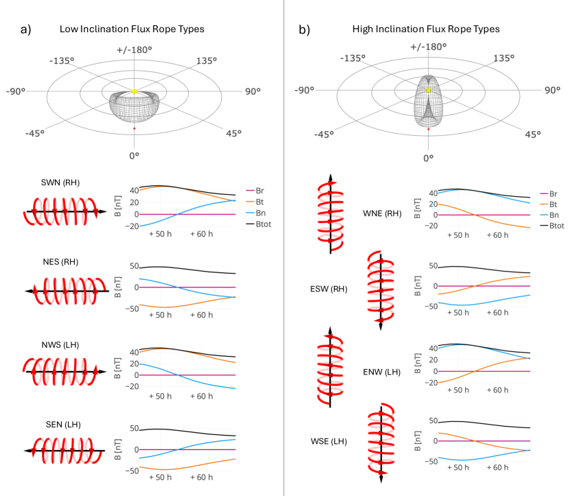
Figure 1: Graphic representation of the eight flux rope types: a) low inclination flux rope types, and b) high inclination flux rope types. A 3DCORE model is shown at the top for both low and high inclinations, and the simplified sketches of the flux ropes together with the in situ profiles for an apex hit for each flux rope type are visualised below. Each flux rope type is labelled next to the corresponding sketch, along with its handedness (LH: left-handed, RH: right-handed).

The global structure of CMEs is believed to have both ends of the flux rope connected to the Sun for a considerable duration during its propagation through the heliosphere, as suggested by the presence of bidirectional electron flows in some CMEs up to 1 au (e.g. Richardson, 1997; Shodhan et al., 2000). Nevertheless, while Zurbuchen & Richardson (2006) proposed the legs of a CME to contain highly twisted field lines, Owens (2016) suggested the existence of “legs” of untwisted magnetic flux. This theory might serve as an additional explanation for the appearance of ICME signatures that deviate from the ideal flux rope signatures.

Although relatively rare, measurements of the same ICME by spacecraft at multiple points over varying heliocentric distances and longitudinal separations have provided valuable insights into their structural characteristics. While there is a general consistency with the helical flux rope (FR) model, it is noteworthy that not all ICMEs exhibit clear FR structures. Different studies have highlighted significant variations among individual ICMEs, deviating from overall statistical trends (for overviews see Kilpua et al., 2009; Good et al., 2018; Lugaz et al., 2018; Salman et al., 2020; Davies et al., 2022). This variability points to possible alterations from the classic flux rope hypothesis, which may be attributed to diverse factors such as interactions with other structures or the the background solar wind, and different spacecraft measurement points and cuts through the ICME (e.g. Möstl et al., 2009, 2012), particularly affecting the flattening of the circular cross section (e.g. Riley & Crooker, 2004; Owens et al., 2006; Savani et al., 2010; Davies et al., 2021). For an overview on these various processes CMEs undergo as they propagate away from the Sun, we refer the reader to Manchester et al. (2017); Luhmann et al. (2020); Temmer et al. (2023).

Regnault et al. (2023) recently highlighted the scarcity of simultaneous multipoint measurements of the same ICME, emphasizing the need for more data to enhance our understanding. Looking ahead, currently operating missions such as Parker Solar Probe, Solar Orbiter, BepiColombo, Wind, and STEREO-A are anticipated to contribute significantly to this field by providing additional multipoint observations. These missions, currently operational within 1 au, offer opportunities to study a broader range of ICME events and further refine our understanding of their complex structures and dynamics.

A subset of magnetic flux ropes that can neither be fitted using the force-free model (Lepping et al., 1990), nor be reconstructed with the Grad-Shafranov technique (Hu & Sonnerup, 2002), are known as “magnetic-cloud-like” (MCL, Lepping et al., 2006) ejecta. One special observational signature within these that has puzzled researchers for a long time are so-called “back regions” of ICMEs which follow after the main flux rope rotation has passed the observer. In these regions, the field stays somewhat elevated, but does rotate only very slightly and the field components remain essentially constant. Two explanations have been put forward for this behaviour: (1) magnetic field lines are peeled off from the front of the flux rope through magnetic reconnection as it propagates through the solar wind (e.g. Dasso et al., 2007; Ruffenach et al., 2012), leaving a trail of field lines that point in the same direction behind, or (2) the observer passes through the flux rope in such a way that the constant field arises for a quasi-stationary observer purely from a geometrical effect (Möstl et al., 2010) and is actually part of the flux rope itself. In reality, both processes may contribute to the ICME signature that is then observed by a spacecraft.

Improving modeling capabilities to account for the high complexity of CME propagation and evolution has been a key element of studies within the past years (e.g. Pomoell & Poedts, 2018; Sarkar et al., 2020; Pal et al., 2022; Kay et al., 2023; Maharana et al., 2023). An investigation of the influence of initial parameters of a CME MHD simulation on the results at different latitudinal and longitudinal locations at 1 au has been conducted by Shen et al. (2021). Their study indicated, that as long as the initial mass of the CME remains unchanged, the initial geometric thickness will have a different influence in the latitudinal and longitudinal direction. Scolini et al. (2021) used a swarm of simulated spacecraft in radial alignment to study the development of CME magnetic complexity during propagation, relating the probability of detecting complexity changes to the interaction with large-scale solar wind structures. Similarly, a swarm of synthetic spacecraft at different latitudinal and longitudinal positions was used in Scolini et al. (2023) to study the coherence of CMEs. Their simulations suggest a CME to retain a lower complexity and higher coherence along its magnetic axis, while still requiring crossings along both the axial and perpendicular directions for a characterization of its global complexity. Additionally, coherence is found to be lower in the west flank of the structure, due to Parker spiral effects. A study comparing stationary spacecraft and trajectories similar to Parker Solar Probe in an MHD simulation was conducted by Lynch et al. (2022). Finding in situ flux rope models to be generally applicable for the inference of some physical properties, such as size and flux content, they conclude shortcomings in the determination of the flux rope axis orientation.

In this study, we test two hypotheses. The first hypothesis is that constant, non-rotating (CNR) in situ signatures can be explained by an effect of the trajectory of an observer through a 3D expanding magnetic flux rope, without invoking magnetic reconnection as an explanation for those signatures. Furthermore, we investigate the appearance of different flux rope types for different trajectories. According to Palmerio et al. (2018), only about half of the studied events show a match regarding their flux rope type, when comparing in situ observations to observations from the Sun. Therefore, we attempt to validate or refute the second hypothesis, whether trajectory effects can lead to a misinterpretation of flux rope types.

To this end, we employ the 3DCORE model, which is a 3D magnetic field model for ICME flux ropes first presented by Möstl et al. (2018) and significantly improved by Weiss et al. (2021a, b). By placing up to 20 synthetic spacecraft at 0.8 au and analyzing how their respective positions influence measured in situ signatures, we attempt to gain insight into how CNRs present in ICME in situ signatures can be generated.

In Section 2, we give a short summary of the 3DCORE model in general and report on a new tool called 3DCOREweb, which facilitates its usability. We additionally outline the general setup of the simulation. In Section 3, we show the in situ signatures obtained by spacecraft at different locations, and discuss these in Section 4.

2 Method

2.1 3DCOREweb

3DCORE is a semi-empirical 3D flux rope model, which is described in detail in Weiss et al. (2021a, b). In the past, the model has proven successful in inferring flux rope parameters by fitting in situ magnetic field observations employing an Approximate Bayesian Computation-Sequential Monte Carlo (ABC-SMC) method (e.g. Davies et al., 2021; Telloni et al., 2021; Möstl et al., 2022; Long et al., 2023). In the case of limited longitudinal separations (within $\sim 5^{\circ}$), even multipoint events have successfully been fitted simultaneously (e.g. Davies et al., 2021; Weiss et al., 2021b). 3DCORE assumes a torus-like shape with an embedded Gold-Hoyle-like magnetic field, based on an analytical solution by Vandas & Romashets (2017). The structure is attached to the Sun on both ends and expands self-similarly during its propagation. The interaction with the background solar wind is considered through a simple drag model (Vršnak et al., 2013), allowing for the frontal part of the CME to either be accelerated or decelerated, depending on the relative speed of the ambient solar wind. By including an elliptical cross-section through variation of the aspect ratio, propagation effects like flattening of the flux rope in the direction of propagation (also known as “pancaking”, Riley & Crooker, 2004) are approximated. A more thorough explanation of the mathematical setup of the model and its 13 input parameters can be found in Weiss et al. (2021a, b). These 13 parameters are: longitude, latitude, inclination, diameter at 1 au ($D_{1\mathrm{au}}$), aspect ratio ($\delta$), launch radius ($R_{0}$), launch velocity ($V_{0}$), expansion rate ($n_{a}$), background drag ($\Gamma$), solar wind speed ($V_{sw}$), twist factor ($T_{f}$), magnetic decay rate ($n_{b}$) and magnetic field strength at 1 au ($B_{1\mathrm{au}}$). The magnetic field within the toroidal structure is given for custom curvilinear coordinates ($r\in\lceil 0,\infty)$, $\psi\in\lceil 0,2\pi)$, $\phi\in\lceil 0,2\pi)$) based on the toroidal coordinate system by

$$B_{r} =0$$ (1a)

$$B_{\psi} =\frac{B_{0}}{1+b^{2}r^{2}}$$ (1b)

$$B_{\phi} =\frac{B_{0}br}{(1+b^{2}r^{2})\left(1+r\frac{\rho_{1}}{\rho_{0}}\cos\phi\right)},$$ (1c)

following a Gold-Hoyle-like solution described in Vandas & Romashets (2017), with $B_{0}$ as the magnetic field at the central axis of the toroidal structure and $b$ as a modified twist parameter defined as

$$b=T_{f}\frac{\rho_{1}}{2\pi\rho_{0}}\sin\left(\frac{\psi}{2}\right)^{2}.$$ (2)

where $\rho_{0}$ and $\rho_{1}$ define the major and minor radius of the base torus, while the flux rope structure itself is defined by the implicit volume $r\leq 1$. As defined in Weiss et al. (2021b), the twist factor $T_{f}$ used as input parameter relates to the number of twists $\tau$ as $\tau=T_{f}/E(\delta)$, where $E(\delta)$ is a function for the circumference of an ellipse with a given aspect ratio $\delta$. The scaling laws are implemented according to Leitner et al. (2007) as

$$D(t) =D_{1au}R_{apex}(t)^{n_{a}}$$ (3a)

$$B_{0}(t) =B_{1au}R_{apex}(t)^{-n_{b}},$$ (3b)

including the time dependency. $R_{apex}$ hereby refers to the distance of the CME’s apex point to the Sun.

While the model’s simplicity allows for real-time application as well as the generation of large ensembles, there are some drawbacks which have to be taken into account. Such examples are the fixed flux rope width of $180^{\circ}$, as well as the background solar wind speed which is assumed to be constant throughout the heliosphere. While this implementation still produces sufficiently reasonable results locally, the application to multipoint events has shown that the global large-scale structure is not adequately and realistically enough modelled to overcome large spacecraft separations (Weiss et al., 2021b; Davies et al., 2024). In the past, this has been circumvented by fitting both in situ spacecraft observations separately and retrospectively comparing their results, which has yielded meaningful conclusions, but still has to be considered when analysing and interpreting model results. Additionally, deformations and deflections aside from the flattening of the cross section as well as a non constant twist have not yet been implemented, even though they are already subject to further investigation (Weiss et al., 2022).

Recently, we have made an effort to increase the model’s usability through 3DCOREweb. A Dash (Plotly Technologies Inc., 2015) application is available via GitHub and includes a graphical user interface that can be used without any prior Python knowledge. An example screenshot of this graphical user interface is shown in Figure 2.

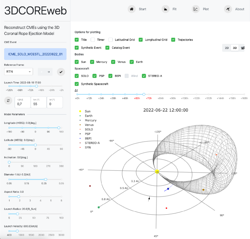
Figure 2: A screenshot of the graphical user interface in 3DCOREweb, as available via GitHub. This screenshot shows the subpage “Plot”, where the user is able to create interactive 3D plots inserting the 3DCORE model into the heliosphere. The panel on the left shows the details of the event, in this case an ICME measured by Solar Orbiter (SOLO) on 2022-06-22. It also contains the sliders to adjust the model input parameters. Above the plot, the user can modify plotting options and visualize the temporal evolution by adjusting the time slider. Furthermore, the user can visualize generated in situ signatures of the model, use the ABC-SMC algorithm as introduced in Weiss et al. (2021a), and analyse the results.

The user can either choose to reconstruct ICME signatures from the HELIO4CAST ICME catalog, an extensive living catalog of interplanetary coronal mass ejections (Möstl et al., 2020), or a custom event for a variety of spacecraft (e.g. Solar Orbiter, Parker Solar Probe, STEREO-A) when the data is pre-downloaded from a given repository. The straightforward implementation of the fitting algorithm as well as a clear overview of the results facilitate the application of the tool for the general scientific community. Additionally, we further exploited the usage of 3DCORE as a simple forward modeling tool, including a large variety of Python routines for modeling, analyzing and plotting.

2.2 Simulation Setup

Figure 3 presents an overview of the experiment setup for a low inclination flux rope, placing 20 synthetic spacecraft at a radial distance of 0.8 au from the Sun. Due to the simplified propagation within the model, we can neglect the radial evolution of the CME in our study. Scolini et al. (2023) similarly reported the lack of increase in magnetic complexity in the absence of interactions with other large-scale structures. The intermediate radial distance of 0.8 au was thus chosen to resemble the magnitude of typical events measured by spacecraft in the inner heliosphere, while still keeping the temporal shift in arrival time within acceptable limits. Their respective positions include five longitudinal (the central meridian with respect to the CME, $\pm 30^{\circ}$, $+45^{\circ}$ and $+60^{\circ}$) and four latitudinal planes (at the solar equatorial plane, $\pm 5^{\circ}$, and $+15^{\circ}$). These are visualized by different colors representing different latitudinal planes, as well as different symbols for different longitudinal planes. The asymmetry of the spacecraft distribution was chosen due to the inherent symmetry of the structure introducing redundancy in the results.

Figure 4 shows the simulation setup similarly for a high inclination flux rope, with 16 spacecraft in four longitudinal (the central meridian with respect to the CME, $\pm 5^{\circ}$ and $+15^{\circ}$) and four latitudinal planes (at the solar equatorial plane, $\pm 30^{\circ}$, and $+45^{\circ}$), also at a radial distance of 0.8 au from the Sun. Since the longitudinal extension of the high inclination flux rope is much smaller than for the low inclination flux rope, fewer longitudinal planes are included, while the four latitudinal planes are stretched out to account for the higher latitudinal extension in this case.

The initial parameters as used for the model in 3DCOREweb are shown in Table 1. While inclination and twist are varied accordingly to produce the eight different flux rope types (see Table 2), the other parameters are kept to generic standard values to better compare the influence of the observers’ locations. Due to the model setup, inclination values of $0^{\circ}$ and $180^{\circ}$ correspond to low inclination flux ropes with their central axis pointing in opposite directions, while inclination values of $90^{\circ}$ and $270^{\circ}$ lead to both orientations of high inclination flux ropes. For the flux rope example in this study, a $T_{f}=50$ corresponds to a high twist number of $\tau\approx 5$ turns and a $T_{f}=5$ corresponds to a low twist number of $\tau\approx 0.5$ turns, with the twist number $\tau$ corresponding to the total number of twists along the entire torus. These numbers are chosen in agreement with Kahler et al. (2011), who estimated the number of field line rotations over the assumed CME full length to be 1–10 turns. A visualization of a single field line for both low and high twist CME can be seen in Figure 5, where the low twist field line is represented in blue, and the high twist in red.

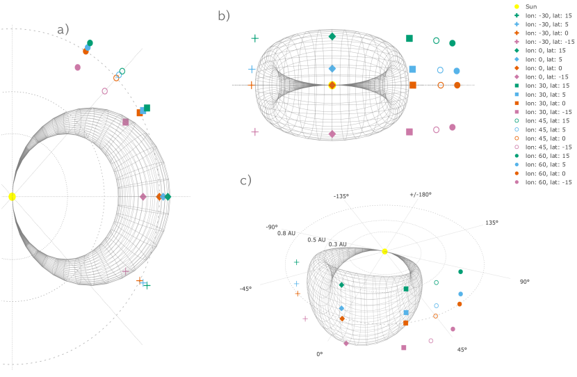
Figure 3: Synthetic spacecraft setup for the low inclination flux rope, shown from three different viewing angles: a) top view down from solar equatorial north, b) front view from the apex of the structure along the solar equatorial plane, c) angled view. Spacecraft positions include five longitudinal (the central meridian with respect to the CME, $\pm 30^{\circ}$, $+45^{\circ}$, and $+60^{\circ}$) and four latitudinal planes (at the solar equatorial plane, $\pm 5^{\circ}$, and $+15^{\circ}$) at 0.8 au radial distance from the Sun.

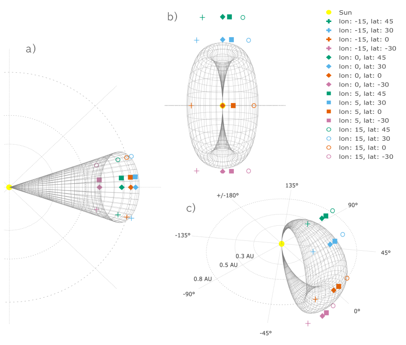
Figure 4: Synthetic spacecraft setup for the high inclination flux rope, shown from three different viewing angles: a) top view down from solar equatorial north, b) front view from the apex of the structure along the solar equatorial plane, c) angled view. Spacecraft positions include four longitudinal (the central meridian with respect to the CME, $\pm 5^{\circ}$, and $+15^{\circ}$) and four latitudinal planes (at the solar equatorial plane, $\pm 30^{\circ}$, and $+45^{\circ}$) at 0.8 au radial distance from the Sun.

Table 1: Model parameters (longitude, latitude, inclination, diameter at 1 au ($D_{1\mathrm{au}}$), aspect ratio ($\delta$), launch radius ($R_{0}$), launch velocity ($V_{0}$), expansion rate ($n_{a}$), background drag ($\Gamma$), solar wind speed ($V_{sw}$), twist factor ($T_{f}$), magnetic decay ($n_{b}$), magnetic field strength at 1 au ($B_{1\mathrm{AU}}$)) for low inclination and high inclination flux ropes with low and high $T_{f}$. The longitude and latitude of the flux rope are given in HEEQ coordinates.

Parameters	Values	Units
Longitude	$0.$	deg
Latitude	$0.$	deg
Inclination	$0.$ / $90.$ / $180.$ / $270.$	deg
$D_{1\mathrm{AU}}$	$0.3$	au
$\delta$	$2.$
$R_{0}$	$20.$	solar radii
$V_{0}$	$600.$	km/s
$n_{a}$	$1.14$
$\Gamma$	$1.$
$V_{\mathrm{sw}}$	$500.$	km/s
$T_{f}$	$50.$ / $5.$ / $-5.$ / $-50.$
$n_{b}$	$1.64$
$B_{1\mathrm{au}}$	$25.$	nT

Table 2: Inclination and $T_{f}$ as set in the 3DCORE model for different flux rope types including both low and high twist values.

Flux rope type	Handedness	Inclination [deg]	$T_{f}$
SWN	Right-handed	$180.$	$5.$/$50.$
NES	Right-handed	$0.$	$5.$/$50.$
NWS	Left-handed	$180.$	$-5.$/$-50.$
SEN	Left-handed	$0.$	$-5.$/$-50.$
WNE	Right-handed	$270.$	$5.$/$50.$
ESW	Right-handed	$90.$	$5.$/$50.$
ENW	Left-handed	$270.$	$-5.$/$-50.$
WSE	Left-handed	$90.$	$-5.$/$-50.$

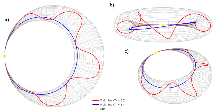
Figure 5: A visualization of two field lines within the CME shape for high twist of $T_{f}=50$ (red) and low twist of $T_{f}=5$ (blue).

By comparing the resulting in situ profiles, we investigate which circumstances lead to CNRs. More precisely, we analyse the influence of flux rope type, twist parameter and observer location on the measured in situ signatures. Furthermore, we attempt to show whether flux rope types can be unambiguously distinguished.

3 Comparison of Signatures

Figures 6 – 9 show the results. Each figure presents the synthetic in situ measurements for a specific flux rope type as measured by the observers described in Section 2.2. Each subplot coincides with one spacecraft, with each row representing a different latitude and each column representing a different longitude. The vertical axis shows the magnetic field $B(t)$ in nT and the horizontal axis indicates the time that has passed since the launch of the CME in hours. All three magnetic field components (radial $B_{r}$, tangential $B_{t}$, normal $B_{n}$), as well as the total magnetic field ($B_{tot}$) are shown in RTN coordinates. We have chosen one low inclination and one high inclination flux rope type, both with low twist and high twist configurations, as the general tendencies of how the signatures change upon varying longitude and latitude are the same for each low/high flux rope type and only differ regarding its handedness. Nevertheless, these figures have been created for all flux rope types for completeness and can be found in the Appendix.

3.1 High Twist Flux Ropes

Figure 6 shows the results for a low inclination and high twist SWN flux rope type. As expected, the in situ signatures exhibit a bipolar $B_{n}$ component, changing sign from negative (South) to positive (North), and a unipolar $B_{t}$ component that stays positive (West).

Varying the spacecraft longitude from $-30^{\circ}$ to $+60^{\circ}$, $B_{r}$ shifts from positive to negative. Similar behaviour can also be observed when varying latitude, with a negative latitude corresponding to a negative $B_{r}$ component and a positive latitude corresponding to a positive $B_{r}$. The $B_{r}$ component stays 0 for the apex hit at both longitude and latitude equal to 0. This pattern is also observed in other classic flux rope models such as the Lundquist model, where the deviation of $B_{r}$ away from 0 gives a sense of the distance of the spacecraft from the flux rope axis, otherwise known as the impact parameter (Good et al., 2018; Lepping et al., 1990, 2006). Additionally, moving from the apex to the flanks of the CME, the profile gets stretched in time and the total change of the values in all components becomes smaller. For the flank encounters, high latitudes do not measure any signatures as the CME does not hit a synthetic spacecraft at that point, as expected. Additionally, a larger radial width of the CME is traversed for a latitude of $0^{\circ}$ compared to high latitudes. The high twist of the flux rope is reflected in the significant rotation of the magnetic field vector leading to a variation in all three components for apex hits and still a considerable variation in $B_{n}$ for flank encounters, even though the overall profile is notably stretched and flattened. In the extreme cases of a latitude of $-15^{\circ}$ combined with a longitude of $30^{\circ}$ or a latitude of $15^{\circ}$ combined with a longitude of $-30^{\circ}$, $B_{t}$ is observed very close to 0.

Interestingly, the total magnetic field increases significantly for flank hits. While the observed effect arises from the tapering of the torus shape, resulting in an inverse relationship between the torus radius and magnetic field strength, the validity of this assumption may be refined through future investigations into multipoint events.

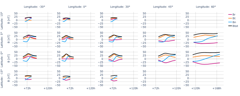
Figure 6: In situ measurements of the synthetic spacecraft in different latitudes and longitudes for a low inclination and high twist SWN type flux rope. For better comparison of the times of arrival, the x-axis displays the same time range for all subplots except for a longitude of $60^{\circ}$.

Figure 7 shows a high inclination and high twist WNE flux rope type. The high inclination of the flux rope can be seen in the bipolarity of $B_{t}$, changing sign from positive (West) to negative (East), and the unipolarity of $B_{n}$, staying positive (North).

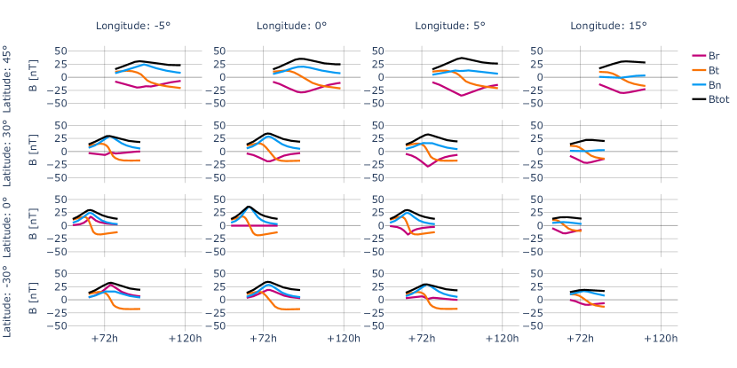
Figure 7: In situ measurements of the synthetic spacecraft in different latitudes and longitudes for a high inclination and high twist WNE type flux rope. For better comparison of the times of arrival, the x-axis displays the same time range for all subplots.

Keeping in mind that in the high inclination case, high latitudes correspond to flank encounters, while the spacecraft in the solar equatorial plane experience apex hits, we observe similar patterns as for the low inclination flux rope types, with flank encounters producing considerably flatter in situ profiles compared to the apex hits.

Interestingly, we observe no CNRs for any of the high twist flux rope types, even for flank hits. While the unipolar components show a less significant variation for flank hits, the bipolarity of $B_{t}$ is conserved throughout the whole structure. As a result, the components analysed for the determination of the flux rope types are unambiguous, regardless of where the CME hits the spacecraft. Nevertheless, we observe some extreme cases for which the unipolar component is observed very close to 0 which might lead to a misclassification of the flux rope type.

3.2 Low Twist Flux Ropes

Figures 8 and 9 show the low twist counterparts to Figures 6 and 7. Figure 8 shows the results for a low inclination and low twist SWN flux rope type. The low twist of the flux rope leads to a very minor rotation of the magnetic field. Compared to the pronounced bipolarity of $B_{n}$ for the high twist SWN flux rope, only a very minor change from slightly negative to slightly positive can be observed in this plot. Nevertheless, as $B_{t}$ appears very flat, it is constantly positive and has a greater difference to 0 than for the high twist counter part.

While apex hits already show very flat signatures, we observe CNRs for flank hits. As for the high twist flux ropes, the total magnetic field is significantly higher for flank hits.

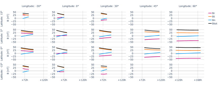
Figure 8: In situ measurements of the synthetic spacecraft in different latitudes and longitudes for a low inclination and low twist SWN type flux rope. For better comparison of the times of arrival, the x-axis displays the same time range for all subplots except for a longitude of $60^{\circ}$.

Figure 9 shows a high inclination and low twist WNE flux rope type. The high inclination of the flux rope can once again be identified by the bipolarity of $B_{t}$, changing sign from positive to negative, and the unipolarity of $B_{n}$, staying positive. Nevertheless, as for the low twist SWN type, the observed bipolarity is very minor.

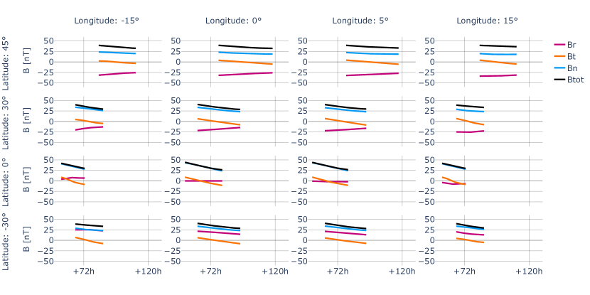
Figure 9: In situ measurements of the synthetic spacecraft in different latitudes and longitudes for a high inclination and low twist WNE type flux rope. For better comparison of the times of arrival, the x-axis displays the same time range for all subplots.

As for all low inclination, low twist types, flank encounters produce considerably flatter in situ profiles compared to the apex hits, leading to CNR signatures. This makes a distinction of flux rope types based on in situ signatures difficult, even for perfectly radial encounters.

4 Discussion and Conclusions

In this study, we investigated the effect of the position of a synthetic spacecraft and the resulting trajectory at different latitudinal and longitudinal locations at 0.8 au on the in situ magnetic field signatures observed using 3DCOREweb. We investigated hypothesis 1, whether trajectory effects could be a possible explanation for the observation of CNRs. We discover that for a high twist CME, a flank hit results in a very flat in situ profile with two out of three components not exhibiting a visible variation that would indicate a rotation of the magnetic field vector. Nevertheless, the third component still displays a bipolar signature, although it is much flatter than observed for an apex hit. To observe a CNR, the CME had to be initialized with a low twist and a flank hit had to be simulated. Relating our findings to the general context of whether the legs of a CME might contain twisted field lines, as studied in Owens (2016), further investigation of multipoint events will be needed. While our initial findings suggest that observing a constant field for a flank impact implies minimal twisting within its legs, confirming this requires simultaneous measurements at the apex. This would solidify whether the observed CME’s structure has varying levels of twist throughout, rather than assuming it to be a generally low twist CME.

This also points out an obvious drawback of our model, namely the constant twist and its non-deformable shape. The opening angle of $180^{\circ}$ prevents the modeling of a trajectory that experiences both an apex hit and a flank encounter for the same CME. Keeping in mind that CMEs are thought to be generally deformable structures (e.g. Manchester et al., 2017; Kilpua et al., 2019; Luhmann et al., 2020), which may deviate strongly from our idealized shape and thus in reality quite often experience such scenarios, limits the accuracy of our model. Nevertheless, the separate analysis of flank encounters and apex hits ties in with the possible explanation of trajectory effects causing CNR signatures.

In the past, intrinsic flux rope types, as identified in solar signatures, have often not matched the in situ flux rope types identified as investigated in e.g. Palmerio et al. (2018). Throughout this work, we compared in situ results for different flux rope types and investigated hypothesis 2, whether flux rope types could be misinterpreted due to non-apex hits. For a low twist CME, it appeared indeed to be challenging to identify the flux rope type, due to CNRs observed for flank hits. Nevertheless, for high twist CMEs, the flux rope type could be unambiguously assigned, regardless of where the impact occurred, unless one of the identified rare cases of an almost 0 unipolar component occurred. While this hints towards the need for alternative explanations for the mismatching of flux rope types from solar to in situ observations, we have to consider that our model poses some very general assumptions. For a deformable CME, as well as non-frontal encounters, this could nonetheless be explained by trajectories and needs to be further investigated. For a highly deformed flux rope, a spacecraft could potentially be impacted by the front part of a CME, followed directly by a flank encounter. In comparison to that, the self-similar expansion implemented in our model combined with a stationary spacecraft leads to a highly idealized frontal encounter with the flux rope, which might only partially model reality. Especially for spacecraft in close proximity to the Sun, such as Parker Solar Probe, a rapidly changing spacecraft position may have to be taken into account when analysing CME encounters. Nevertheless, this has been studied in Möstl et al. (2020) and the effect turned out to be negligible, but only for one particular type of encounter.

To further corroborate the validity of our results, we are awaiting the possible occurrence of many more multipoint measurements in the near future. Especially with Solar Orbiter due to commence probing higher latitudes and the general increase in spacecraft measuring the solar wind, including the future operational space weather mission Vigil, planned for launch by ESA in 2031, as well as the approach of the maximum of solar cycle 25, statistical studies will hopefully be facilitated.

Throughout this work, we confirm the substantial impact of both latitudinal and longitudinal positions of spacecraft on the appearance of in situ signatures. These results could significantly aid in future analysis of in situ data, such as concluding the relative trajectory of the spacecraft through the CME with respect to its propagation direction, as well as its flux rope type.

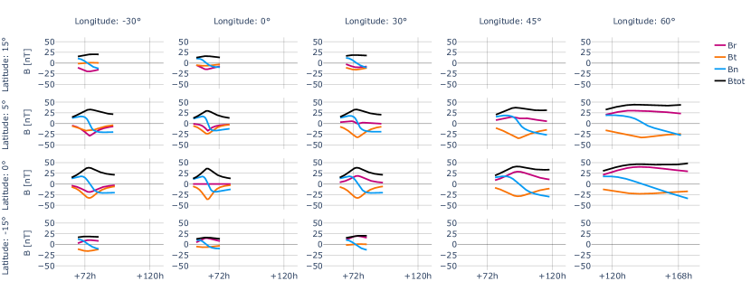
Figure 10: In situ measurements of the synthetic spacecraft in different latitudes and longitudes for a low inclination and high twist NES type flux rope. For better comparison of the times of arrival, the x-axis displays the same time range for all subplots except for a longitude of $60^{\circ}$.

Figures 11 and 12 show the left-handed counterparts NWS and SEN to these, where the NWS type exhibits $B_{n}$ changing sign from positive to negative and $B_{t}$ remaining positive, while the SEN type has $B_{n}$ changing sign from negative to positive and $B_{t}$ remaining negative.

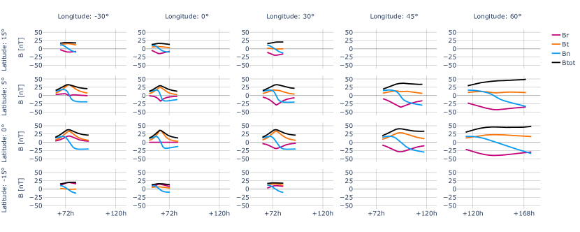
Figure 11: In situ measurements of the synthetic spacecraft in different latitudes and longitudes for a low inclination and high twist NWS type flux rope. For better comparison of the times of arrival, the x-axis displays the same time range for all subplots except for a longitude of $60^{\circ}$.

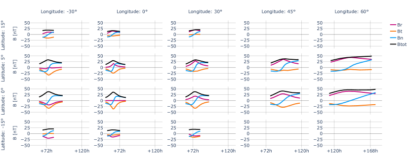
Figure 12: In situ measurements of the synthetic spacecraft in different latitudes and longitudes for a low inclination and high twist SEN type flux rope. For better comparison of the times of arrival, the x-axis displays the same time range for all subplots except for a longitude of $60^{\circ}$.

The second right-handed high inclination flux rope type is shown in Figure 13, for which $B_{t}$ changes sign from negative to positive and $B_{n}$ remains negative.

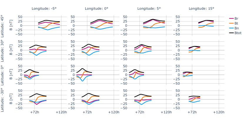
Figure 13: In situ measurements of the synthetic spacecraft in different latitudes and longitudes for a high inclination and high twist ESW type flux rope. For better comparison of the times of arrival, the x-axis displays the same time range for all subplots.

Figures 14 and 15 show the left-handed counterparts to these, where the ENW type exhibits $B_{t}$ changing sign from negative to positive and $B_{n}$ remaining positive, while the WSE type has $B_{t}$ changing sign from positive to negative and $B_{n}$ remaining negative.

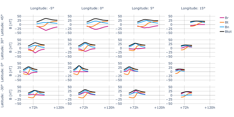
Figure 14: In situ measurements of the synthetic spacecraft in different latitudes and longitudes for a high inclination and high twist ENW type flux rope. For better comparison of the times of arrival, the x-axis displays the same time range for all subplots.

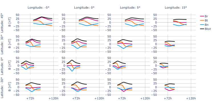
Figure 15: In situ measurements of the synthetic spacecraft in different latitudes and longitudes for a high inclination and high twist WSE type flux rope. For better comparison of the times of arrival, the x-axis displays the same time range for all subplots.

Figure 16 shows the second right-handed low inclination flux rope type NES $B_{n}$ changes sign from slightly positive to slightly negative and $B_{t}$ remains negative.

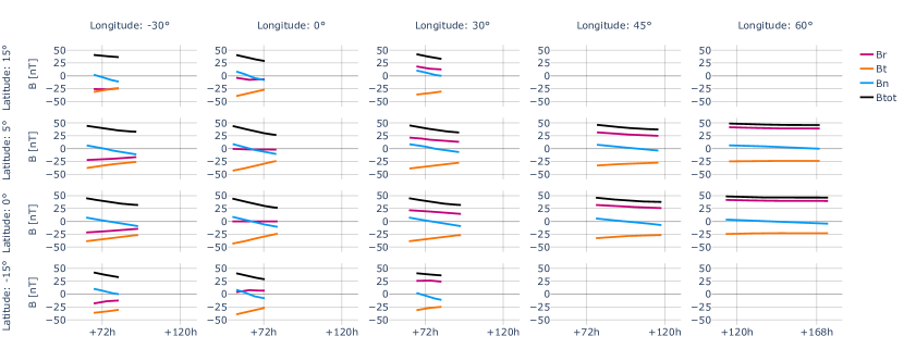
Figure 16: In situ measurements of the synthetic spacecraft in different latitudes and longitudes for a low inclination and low twist NES type flux rope. For better comparison of the times of arrival, the x-axis displays the same time range for all subplots except for a longitude of $60^{\circ}$.

Figures 17 and 18 show the left-handed counterparts to these, where the NWS type exhibits $B_{n}$ changing sign from slightly positive to slightly negative and $B_{t}$ remaining positive, while the SEN type has $B_{n}$ changing sign from slightly negative to slightly positive and $B_{t}$ remaining negative.

Figure 17: In situ measurements of the synthetic spacecraft in different latitudes and longitudes for a low inclination and low twist NWS type flux rope. For better comparison of the times of arrival, the x-axis displays the same time range for all subplots except for a longitude of $60^{\circ}$.

Figure 18: In situ measurements of the synthetic spacecraft in different latitudes and longitudes for a low inclination and low twist SEN type flux rope. For better comparison of the times of arrival, the x-axis displays the same time range for all subplots except for a longitude of $60^{\circ}$.

The second right-handed high inclination flux rope type is shown in Figure 19, for which $B_{t}$ changes sign from slightly negative to slightly positive and $B_{t}$ remains negative.

Figure 19: In situ measurements of the synthetic spacecraft in different latitudes and longitudes for a high inclination and low twist ESW type flux rope. For better comparison of the times of arrival, the x-axis displays the same time range for all subplots.

Figures 20 and 21 show the left-handed counterparts to these, where the ENW type exhibits $B_{t}$ changing sign from slightly negative to slightly positive and $B_{n}$ remaining positive, while the WSE type has $B_{t}$ changing sign from slightly positive to slightly negative and $B_{n}$ remaining negative.

Figure 20: In situ measurements of the synthetic spacecraft in different latitudes and longitudes for a high inclination and low twist ENW type flux rope. For better comparison of the times of arrival, the x-axis displays the same time range for all subplots.

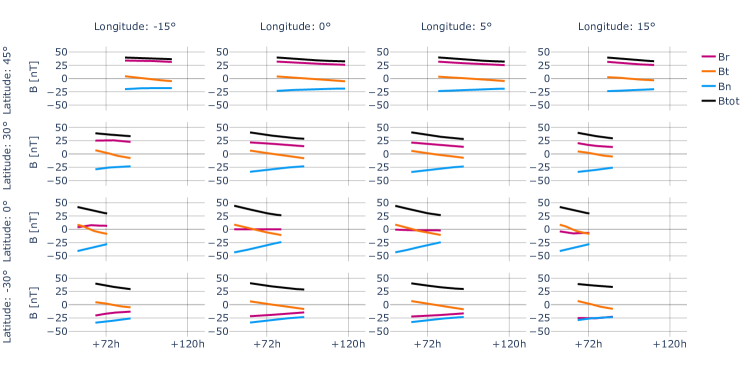
Figure 21: In situ measurements of the synthetic spacecraft in different latitudes and longitudes for a high inclination and low twist WSE type flux rope. For better comparison of the times of arrival, the x-axis displays the same time range for all subplots.

References

- Al-Haddad et al. (2019) Al-Haddad, N., Lugaz, N., Poedts, S., et al. 2019, ApJ, 884, 179, doi: 10.3847/1538-4357/ab4126
- Al-Haddad et al. (2013) Al-Haddad, N., Nieves-Chinchilla, T., Savani, N. P., et al. 2013, Sol. Phys., 284, 129, doi: 10.1007/s11207-013-0244-5
- Bothmer & Schwenn (1998) Bothmer, V., & Schwenn, R. 1998, Ann. Geophys., 16, 1, doi: 10.1007/s00585-997-0001-x
- Burlaga (1988) Burlaga, L. 1988, Journal of Geophysical Research: Space Physics, 93, 7217
- Burlaga et al. (1981) Burlaga, L., Sittler, E., Mariani, F., & Schwenn, a. R. 1981, Journal of Geophysical Research: Space Physics, 86, 6673
- Dasso et al. (2007) Dasso, S., Nakwacki, M. S., Démoulin, P., & Mandrini, C. H. 2007, Sol. Phys., 244, 115, doi: 10.1007/s11207-007-9034-2
- Davies et al. (2022) Davies, E. E., Winslow, R. M., Scolini, C., et al. 2022, ApJ, 933, 127, doi: 10.3847/1538-4357/ac731a
- Davies et al. (2021) Davies, E. E., Möstl, C., Owens, M. J., et al. 2021, A&A, 656, A2, doi: 10.1051/0004-6361/202040113
- Davies et al. (2024) Davies, E. E., Amerstorfer, U. V., Rüdisser, H. T., et al. 2024, ApJ
- Farrugia et al. (1995) Farrugia, C. J., Osherovich, V. A., & Burlaga, L. F. 1995, J. Geophys. Res., 100, 12293, doi: 10.1029/95JA00272
- Gold & Hoyle (1960) Gold, T., & Hoyle, F. 1960, MNRAS, 120, 89, doi: 10.1093/mnras/120.2.89
- Good et al. (2018) Good, S. W., Forsyth, R. J., Eastwood, J. P., & Möstl, C. 2018, Sol. Phys., 293, 52, doi: 10.1007/s11207-018-1264-y
- Hidalgo & Nieves-Chinchilla (2012) Hidalgo, M. A., & Nieves-Chinchilla, T. 2012, ApJ, 748, 109, doi: 10.1088/0004-637X/748/2/109
- Hu & Sonnerup (2002) Hu, Q., & Sonnerup, B. U. Ö. 2002, Journal of Geophysical Research (Space Physics), 107, 1142, doi: 10.1029/2001JA000293
- Isavnin (2016) Isavnin, A. 2016, ApJ, 833, 267, doi: 10.3847/1538-4357/833/2/267
- Kahler et al. (2011) Kahler, S. W., Haggerty, D. K., & Richardson, I. G. 2011, The Astrophysical Journal, 736, 106, doi: 10.1088/0004-637X/736/2/106
- Kay et al. (2023) Kay, C., Nieves-Chinchilla, T., Hofmeister, S. J., Palmerio, E., & Ledvina, V. E. 2023, Space Weather, 21, e2023SW003647, doi: https://doi.org/10.1029/2023SW003647
- Kilpua et al. (2009) Kilpua, E. K. J., Liewer, P. C., Farrugia, C., et al. 2009, Sol. Phys., 254, 325, doi: 10.1007/s11207-008-9300-y
- Kilpua et al. (2019) Kilpua, E. K. J., Good, S. W., Palmerio, E., et al. 2019, Front. Astron. Space Sci., 6, 50, doi: 10.3389/fspas.2019.00050
- Leitner et al. (2007) Leitner, M., Farrugia, C. J., Möstl, C., et al. 2007, J. Geophys. Res.(Space Physics), 112, A06113, doi: 10.1029/2006JA011940
- Lepping et al. (2006) Lepping, R. P., Berdichevsky, D. B., Wu, C. C., et al. 2006, Annales Geophysicae, 24, 215, doi: 10.5194/angeo-24-215-2006
- Lepping et al. (1990) Lepping, R. P., Jones, J. A., & Burlaga, L. F. 1990, J. Geophys. Res., 95, 11957, doi: 10.1029/JA095iA08p11957
- Long et al. (2023) Long, D. M., Green, L. M., Pecora, F., et al. 2023, The Astrophysical Journal, 955, 152, doi: 10.3847/1538-4357/acefd5
- Lugaz et al. (2018) Lugaz, N., Farrugia, C. J., Winslow, R. M., et al. 2018, ApJ, 864, L7, doi: 10.3847/2041-8213/aad9f4
- Luhmann et al. (2020) Luhmann, J. G., Gopalswamy, N., Jian, L. K., & Lugaz, N. 2020, Sol. Phys., 295, 61, doi: 10.1007/s11207-020-01624-0
- Lundquist (1950) Lundquist, S. 1950, Ark. Fys., 2, 361
- Lynch et al. (2022) Lynch, B. J., Al-Haddad, N., Yu, W., Palmerio, E., & Lugaz, N. 2022, Advances in Space Research, 70, 1614, doi: 10.1016/j.asr.2022.05.004
- Maharana et al. (2023) Maharana, A., Plets, K., Isavnin, A., & Poedts, S. 2023, arXiv e-prints, arXiv:2310.11402, doi: 10.48550/arXiv.2310.11402
- Manchester et al. (2017) Manchester, W., Kilpua, E. K. J., Liu, Y. D., et al. 2017, Space Sci. Rev., 212, 1159, doi: 10.1007/s11214-017-0394-0
- Marubashi (1986) Marubashi, K. 1986, Advances in Space Research, 6, 335, doi: 10.1016/0273-1177(86)90172-9
- Möstl et al. (2020) Möstl, C., Weiss, A., Bailey, R., & Reiss, M. 2020, HELCATS Interplanetary Coronal Mass Ejection Catalog v2.0, figshare, doi: 10.6084/m9.figshare.6356420.v7
- Möstl et al. (2009) Möstl, C., Farrugia, C. J., Miklenic, C., et al. 2009, J. Geophys. Res., 114, A04102, doi: 10.1029/2008JA013657
- Möstl et al. (2010) Möstl, C., Temmer, M., Rollett, T., et al. 2010, Geophys. Res. Lett., 37, L24103, doi: 10.1029/2010GL045175
- Möstl et al. (2012) Möstl, C., Farrugia, C. J., Kilpua, E. K. J., et al. 2012, ApJ, 758, 10, doi: 10.1088/0004-637X/758/1/10
- Möstl et al. (2018) Möstl, C., Amerstorfer, T., Palmerio, E., et al. 2018, Space Weather, 16, 216, doi: 10.1002/2017SW001735
- Möstl et al. (2020) Möstl, C., Weiss, A. J., Bailey, R. L., et al. 2020, ApJ, 903, 92, doi: 10.3847/1538-4357/abb9a1
- Mulligan et al. (1998) Mulligan, T., Russell, C. T., & Luhmann, J. G. 1998, Geophys. Res. Lett., 25, 2959, doi: 10.1029/98GL01302
- Möstl et al. (2022) Möstl, C., Weiss, A. J., Reiss, M. A., et al. 2022, The Astrophysical Journal Letters, 924, L6, doi: 10.3847/2041-8213/ac42d0
- Nieves-Chinchilla et al. (2020) Nieves-Chinchilla, T., Szabo, A., Korreck, K. E., et al. 2020, ApJS, 246, 63, doi: 10.3847/1538-4365/ab61f5
- Owens (2016) Owens, M. J. 2016, ApJ, 818, 197, doi: 10.3847/0004-637X/818/2/197
- Owens et al. (2006) Owens, M. J., Merkin, V. G., & Riley, P. 2006, J. Geophys. Res.(Space Physics), 111, A03104, doi: 10.1029/2005JA011460
- Pal et al. (2022) Pal, S., Nandy, D., & Kilpua, E. K. J. 2022, A&A, 665, A110, doi: 10.1051/0004-6361/202243513
- Palmerio et al. (2018) Palmerio, E., Kilpua, E. K. J., Möstl, C., et al. 2018, Space Weather, 16, 442, doi: 10.1002/2017SW001767
- Plotly Technologies Inc. (2015) Plotly Technologies Inc. 2015, Collaborative data science, Montreal, QC: Plotly Technologies Inc. https://plot.ly
- Pomoell & Poedts (2018) Pomoell, J., & Poedts, S. 2018, J. Space Weather Space Clim., 8, A35, doi: 10.1051/swsc/2018020
- Regnault et al. (2023) Regnault, F., Al-Haddad, N., Lugaz, N., et al. 2023, The Astrophysical Journal, 957, 49, doi: 10.3847/1538-4357/acef16
- Richardson (1997) Richardson, I. G. 1997, Geophysical Monograph Series, 99, 189, doi: 10.1029/GM099p0189
- Riley & Crooker (2004) Riley, P., & Crooker, N. U. 2004, ApJ, 600, 1035, doi: 10.1086/379974
- Rouillard et al. (2020) Rouillard, A. P., Poirier, N., Lavarra, M., et al. 2020, ApJS, 246, 72, doi: 10.3847/1538-4365/ab6610
- Ruffenach et al. (2012) Ruffenach, A., Lavraud, B., Owens, M. J., et al. 2012, J. Geophys. Res.(Space Physics), 117, A09101, doi: 10.1029/2012JA017624
- Salman et al. (2020) Salman, T. M., Winslow, R. M., & Lugaz, N. 2020, J. Geophys. Res.(Space Physics), 125, e27084, doi: 10.1029/2019JA027084
- Sarkar et al. (2020) Sarkar, R., Gopalswamy, N., & Srivastava, N. 2020, ApJ, 888, 121, doi: 10.3847/1538-4357/ab5fd7
- Savani et al. (2010) Savani, N. P., Owens, M. J., Rouillard, A. P., Forsyth, R. J., & Davies, J. A. 2010, ApJ, 714, L128, doi: 10.1088/2041-8205/714/1/L128
- Scolini et al. (2021) Scolini, C., Winslow, R. M., Lugaz, N., & Poedts, S. 2021, The Astrophysical Journal Letters, 916, L15, doi: 10.3847/2041-8213/ac0d58
- Scolini et al. (2023) —. 2023, The Astrophysical Journal, 944, 46, doi: 10.3847/1538-4357/aca893
- Shen et al. (2021) Shen, F., Liu, Y., & Yang, Y. 2021, ApJ, 915, 30, doi: 10.3847/1538-4357/ac004e
- Shodhan et al. (2000) Shodhan, S., Crooker, N. U., Kahler, S. W., et al. 2000, J. Geophys. Res., 105, 27261, doi: 10.1029/2000JA000060
- Telloni et al. (2021) Telloni, D., Scolini, C., Möstl, C., et al. 2021, A&A, 656, a5, doi: 10.1051/0004-6361/202140648
- Temmer et al. (2023) Temmer, M., Scolini, C., Richardson, I. G., et al. 2023, arXiv e-prints, arXiv:2308.04851, doi: 10.48550/arXiv.2308.04851
- Vandas & Romashets (2017) Vandas, M., & Romashets, E. 2017, A&A, 608, A118, doi: 10.1051/0004-6361/201731412
- Vršnak et al. (2013) Vršnak, B., Žic, T., Vrbanec, D., et al. 2013, Sol. Phys., 285, 295, doi: 10.1007/s11207-012-0035-4
- Weiss et al. (2021a) Weiss, A. J., Möstl, C., Amerstorfer, T., et al. 2021a, ApJS, 252, 9
- Weiss et al. (2022) Weiss, A. J., Nieves-Chinchilla, T., Möstl, C., et al. 2022, Journal of Geophysical Research: Space Physics, 127, e2022JA030898, doi: https://doi.org/10.1029/2022JA030898
- Weiss et al. (2021b) Weiss, A. J., Möstl, C., Davies, E. E., et al. 2021b, A&A, 656, A13, doi: 10.1051/0004-6361/202140919
- Zurbuchen & Richardson (2006) Zurbuchen, T. H., & Richardson, I. G. 2006, Space Sci. Rev., 123, 31, doi: 10.1007/s11214-006-9010-4