Ladder top-quark condensation imprints in supercooled electroweak phase transition

Abstract

The electroweak (EW) phase transition in the early Universe might be supercooled due to the presence of the classical scale invariance involving Beyond the Standard Model (BSM) sectors and the supercooling could persist down till a later epoch around which the QCD chiral phase transition is supposed to take place. Since this supercooling period keeps masslessness for all the six SM quarks, it has simply been argued that the QCD phase transition is the first order, and so is the EW one. However, not only the QCD coupling but also the top Yukawa and the Higgs quartic couplings get strong at around the QCD scale due to the renormalization group running, hence this scenario is potentially subject to a rigorous nonperturbative analysis. In this work, we employ the ladder Schwinger-Dyson (LSD) analysis based on the Cornwall-Jackiw-Tomboulis formalism at the two-loop level in such a gauge-Higgs-Yukawa system. We show that the chiral broken QCD vacuum emerges with the nonperturbative top condensate and the lightness of all six quarks is guaranteed due to the accidental U(1) axial symmetry presented in the top-Higgs sector. We employ a quark-meson model-like description in the mean field approximation to address the impact on the EW phase transition arising due to the top quark condensation at the QCD phase transition epoch. In the model, the LSD results are encoded to constrain the model parameter space. We then observe the cosmological phase transition of the first-order type and discuss the induced gravitational wave (GW) productions. We find that in addition to the conventional GW signals sourced from an expected BSM at around or over the TeV scale, the dynamical topponium-Higgs system can yield another power spectrum sensitive to the BBO, LISA, and DECIGO, etc.

I Introduction

The QCD phase transition is of particular importance to understand the origin of mass and property for matter, i.e., nucleon. It has extensively been explored so far based on lattice simulations as well as low-energy effective field theories. However, in application to cosmology, the QCD phase transition in the Hubble expanding universe cannot be observed in lattice QCD or experiments today. Therefore, actually, we have little understood the QCD cosmology in the sense of the thermal history of the universe.

The recent and prospected observations of nano hertz gravitational waves (GWs) have the potential sensitivity to deeply clarify the thermal history around the QCD phase transition epoch. The observation of a stochastic GW background has been reported from the NANOGrav pulsar timing array (PTA) collaboration in 15 years of data NANOGrav:2023gor ; NANOGrav:2023hfp . Possible origins of the detected nano Hz peak frequency in a view of the BSM have been investigated also by the NANOGrav collaboration NANOGrav:2023hvm . Other recent PTA data, such as those from the European PTA (EPTA)EPTA:2023sfo ; EPTA:2023akd ; EPTA:2023fyk , Parkes PTA (PPTA)Reardon:2023gzh ; Reardon:2023zen , and Chinese PTA (CPTA) Xu:2023wog have also supported the presence of consistent nano-hertz stochastic GWs. The tail of the GW spectra produced at the QCD phase transition epoch still keeps having a high enough sensitivity also at other interferometers designated aiming at the higher frequency spectra, like the Laser Interferometer Space Antenna (LISA) LISA:2017pwj ; Caprini:2019egz , the Big Bang Observer (BBO) Corbin:2005ny ; Harry:2006fi , and Deci-hertz Interferometer Gravitational Wave Observatory (DECIGO) Kawamura:2006up ; Yagi:2011wg , etc. Thus, such GW evidence is anticipated to provide us with a clue on the new aspect of the QCD cosmology in the thermal history of the universe.

The QCD phase transition has been confirmed to be crossover by the lattice QCD with 2 + 1 flavors at the physical point at the pseudocritical temperature $T_{\rm pc}\sim 155$ MeV Aoki:2009sc ; Borsanyi:2011bn ; Ding:2015ona ; HotQCD:2018pds ; Ding:2020rtq for the chiral phase transition, and at the same time the deconfinement-confinement transition is expected to take place as well Bazavov:2016uvm ; Ding:2017giu . This is the current consensus of the QCD phase transition to our best knowledge. In the Hubble evolutionary universe with BSM, however, the cosmological QCD phase transition might be more involved and richer.

One particular interest is in when the SM is extended to be scale-invariant along with a dark sector, subsequent supercooling including the QCD phase transition can be realized Iso:2017uuu ; Hambye:2018qjv ; vonHarling:2017yew . In this class of the scenario context, the QCD phase transition also plays an important role in triggering the electroweak (EW) phase transition, which can be strong first-order at temperatures $T={\cal O}(T_{\rm pc})$, thus the EW phase transition can be supercooled until then. In the literature several phenomenological and cosmological consequences arising from this non-standard QCD-scale cosmology have been discussed including the impact on the baryogenesis Dichtl:2023xqd ; Ellis:2022lft ; Wang:2022ygk and the gravitational wave detection sensitivities mainly sourced from the scale-invariant dark sector Iso:2017uuu ; Hambye:2018qjv ; Sagunski:2023ynd ; Dichtl:2023xqd ; Frandsen:2022klh ; Ellis:2022lft ; Bodeker:2021mcj ; vonHarling:2017yew

However, the quantum field theory in the thus supercooled epoch may not merely be governed by QCD: the top Yukawa and the Higgs quartic couplings as well as the QCD gauge coupling get strong at around the QCD scale due to the renormalization group running, as plotted in Fig. 1. Hence this scenario is potentially subject to a rigorous nonperturbative analysis, which has never been addressed at this point.

In this paper, we make the first attempt to employ the nonperturbative analysis of the QCD-induced EW phase transition scenario. The method that we apply is the ladder Schwinger-Dyson (LSD) equation based on the Cornwall-Jackiw-Tomboulis (CJT) formalism Cornwall:1974vz at the two-loop level. Working on the gauge-Higgs-Yukawa system including QCD, the Higgs-Yukawa, and the Higgs quartic interactions, we show that the chiral broken QCD vacuum emerges with the nonperturbative top condensate and the lightness of all six quarks is guaranteed. The latter turns out to be due to the accidental U(1) axial symmetry (approximately) present in the top-Higgs Yukawa sector (with small enough EW gauge interactions neglected).

We discuss the impact on the EW phase transition in the thermal history arising from the emergence of the top quark condensation in the QCD phase transition epoch. We monitor the low-energy effective theory by a quark-meson model-like description, for the top - Higgs hybrid system. The nonperturbative scale anomaly induced from the dynamical top mass generation based on the LSD analysis is encoded in the model by the anomaly matching procedure, to constrain the model parameter space. We then observe the cosmological phase transition of the first-order type in the mean field approximation and discuss the associated GW productions. We find that in addition to the conventional GW signals sourced from an expected BSM at around or over the TeV scale, the dynamical topponium-Higgs system can yield another power spectrum sensitive to the BBO, LISA, and DECIGO, etc.

This paper is structured as follows. In Sec. II we start with deriving the SD equations in the gauge-Higgs-Yukawa system relevant to the presently concerned supercooling scalegenesis, and introduce the ladder approximation. In Sec. III, the LSD equations are reproduced in the framework of the CJT formalism at the two-loop level, which also provides the nonperturbative scale anomaly induced from the nontrivial solutions to the LSD equations including the top and Higgs condensates. Then the phase structure with the scale-invariant SM prediction is discussed in detail. In Sec. IV, we model a low-energy description of the present gauge-Higgs-Yukawa theory to be a quark-meson model-like, to discuss the top quark condensation on the effect on the supercooled EW phase in the thermal history. Employing the mean-field approximation, we evaluate the associated cosmological phase transition in the top - Higgs hybrid system and explore the GW production and signals. The summary of the present paper is presented in Section V, along with discussions related to issues to be pursed in the future.

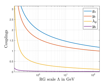
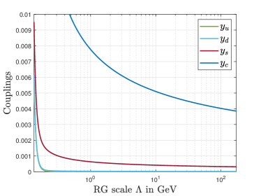
Figure 1: The perturbative two-loop running in the classically scale-invariant SM for the Yukawa couplings (denoted as $y_{f}$ with $f$ being fermion flavor label), the Higgs quartic coupling ($\lambda_{\phi}$), and the QCD gauge coupling $g_{s}$. Here inputs have been made of $m_{h}=125.25$ GeV (the Higgs mass); $v_{\text{EW}}=246$ GeV (the EW scale); $m_{Z}=91.1876$ GeV (the Z boson mass); $\alpha_{s}(m_{Z})(\equiv g_{s}^{2}/(4\pi))=0.1184$ (the $\overline{\text{MS}}$ QCD coupling renormalized at the $m_{Z}$ scale); $m_{t}=172.5$ GeV (the top quark mass); $m_{b}=4.18$ GeV and $m_{c}=1.27$ GeV (the $\overline{\text{MS}}$ masses renormalized at their $\overline{\text{MS}}$ masses); $m_{s}=93.4\times 10^{-3}$ GeV, $m_{d}=4.67\times 10^{-3}$ GeV, and $m_{u}=2.16\times 10^{-3}$ GeV (the $\overline{\text{MS}}$ masses renormalized at 2 GeV). All the inputs above follow the Particle Data Group ParticleDataGroup:2022pth .

II The SD formalism in the gauge - Higgs - Yukawa system: gauge fixing in the ladder approximation

In this section, we derive the exact SD equations in the currently concerned gauge - Higgs - Yukawa system and discuss the ladder truncation. The gauge-Higgs Yukawa system, which dominates the low-energy description of the classically scale-invariant SM, is described by the following Lagrangian:

$$\mathcal{L}=\mathcal{L}_{\text{gauge}}+\mathcal{L}_{\text{quarks}}+\mathcal{L}_{\text{Higgs}}+\mathcal{L}_{\text{Yukawa}},$$ (1)

where

$$\mathcal{L}_{\text{quark}}=i\bar{q_{i}}\left(\not{\partial}+ig_{s}\not{A}\right)q_{i},$$ (2)

$$\mathcal{L}_{\text{Higgs}}=(\partial_{\mu}H)^{\dagger}\partial^{\mu}H-\lambda_{\phi}(H^{\dagger}H)^{2},$$

$$\mathcal{L}_{\text{Yukawa}}=-y_{t}\bar{q_{3}}_{L}\tilde{H}t_{R}-y_{b}\bar{q_{3}}_{L}Hb_{R}+\text{h.c.}\,,$$

and ${\cal L}_{\rm gauge}$ includes the QCD gauge kinetic and Lorentz-covariant gauge fixing terms ($-\frac{1}{2\xi}(\partial_{\mu}A^{a}_{\mu})^{2}$) with the gluon fields $A_{\mu}^{a}$ ($a=1,\cdots,8$) and the gauge fixing parameter $\xi$. In Eq.(1) ${q_{i}}_{L}$ $(i=1,2,3)$ denotes the $i$th generation-$SU(2)_{L}$ quark doublet; $H$ denotes the Higgs doublet parameterized as $H=\left(\begin{array}[]{cc}\phi^{+}\\ \phi^{0}\end{array}\right)=\frac{1}{\sqrt{2}}\left(\begin{array}[]{cc}\pi_{2}-i\pi_{1}\\ \sigma+i\pi_{3}\end{array}\right)$, and its charge conjugate field $\tilde{H}$ is defined as $\tilde{H}\equiv i\tau_{2}H^{*}$ with $\tau_{2}$ being the Pauli matrix. The Higgs (vacuum expectation value) VEV $\sigma_{h}$ arises as $\sigma=\sigma_{h}+\widetilde{\sigma}$, with $\sigma_{h}\equiv\sqrt{2\braket{H^{\dagger}H}}$. Only the third-generation quarks (top and bottom) become strongly coupled to the Higgs as well as to QCD, as seen from the renormalization group evolution in Fig. 1, while other lighter quarks strongly couple only to QCD. The present analysis extends the earlier work in Kondo:1993ty in the sense that the isospin breaking in the Yukawa sector will be taken into account.

II.1 The exact SD equations

From the Lagrangian 1 the exact SD equations for the inverse-full propagators for $t$ and $b$ quark fields, $S_{t}^{-1}$ and $S_{b}^{-1}$, are read off as (for Feynman graphical interpretations, see also Fig. 2)

$$iS_{\text{t}}^{-1} =\not{p}-\frac{y_{t}}{\sqrt{2}}\sigma_{h}-i\int\frac{d^{4}q}{(2\pi)^{4}}\,\frac{-iy_{t}}{\sqrt{2}}S_{\text{t}}(q)\Gamma^{(3)}_{\bar{t}\sigma t}(p,q)\Delta_{\sigma}(p-q)$$

$$\hskip 20.0pt-i\int\frac{d^{4}q}{(2\pi)^{4}}\,\frac{-\gamma_{5}y_{t}}{\sqrt{2}}S_{\text{t}}(q)\Gamma^{(3)}_{\bar{t}\pi_{3}t}(p,q)\Delta_{\pi_{3}}(p-q)$$

$$\hskip 20.0pt-i\int\frac{d^{4}q}{(2\pi)^{4}}\,\frac{-(y_{b}P_{R}-y_{t}P_{L})}{\sqrt{2}}S_{\text{b}}(q)\left[\Gamma^{(3)}_{\bar{b}\pi_{1}t,R}(p,q)+\Gamma^{(3)}_{\bar{b}\pi_{1}t,L}(p,q)\right]\Delta_{\pi_{1}}(p-q)$$

$$\hskip 20.0pt-i\int\frac{d^{4}q}{(2\pi)^{4}}\,\frac{-i(y_{b}P_{R}-y_{t}P_{L})}{\sqrt{2}}S_{\text{b}}(q)\left[\Gamma^{(3)}_{\bar{b}\pi_{2}t,R}(p,q)+\Gamma^{(3)}_{\bar{b}\pi_{2}t,L}(p,q)\right]\Delta_{\pi_{2}}(p-q)$$

$$\hskip 20.0pt-i\int\frac{d^{4}q}{(2\pi)^{4}}\,(-ig_{s}\gamma^{\mu}T^{a})S_{\text{t}}(q)\Gamma^{(3),\nu}_{\bar{t}At,a}(p,q)\Delta_{g,\mu\nu}(p-q)\,,$$ (3)

and

$$iS_{\text{b}}^{-1} =\not{p}-\frac{y_{b}}{\sqrt{2}}\sigma_{h}-i\int\frac{d^{4}q}{(2\pi)^{4}}\,\frac{-iy_{b}}{\sqrt{2}}S_{\text{b}}(q)\Gamma^{(3)}_{\bar{b}\sigma b}(p,q)\Delta_{\sigma}(p-q)$$

$$\hskip 20.0pt-i\int\frac{d^{4}q}{(2\pi)^{4}}\,\frac{\gamma_{5}y_{b}}{\sqrt{2}}S_{\text{b}}(q)\Gamma^{(3)}_{\bar{b}\pi_{3}b}(p,q)\Delta_{\pi_{3}}(p-q)$$

$$\hskip 20.0pt-i\int\frac{d^{4}q}{(2\pi)^{4}}\,\frac{-(y_{t}P_{R}-y_{b}P_{L})}{\sqrt{2}}S_{\text{t}}(q)\left[\Gamma^{(3)}_{\bar{t}\pi_{1}b,R}(p,q)+\Gamma^{(3)}_{\bar{t}\pi_{1}b,L}(p,q)\right]\Delta_{\pi_{1}}(p-q)$$

$$\hskip 20.0pt-i\int\frac{d^{4}q}{(2\pi)^{4}}\,\frac{i(y_{t}P_{R}-y_{b}P_{L})}{\sqrt{2}}S_{\text{t}}(q)\left[\Gamma^{(3)}_{\bar{t}\pi_{2}b,R}(p,q)+\Gamma^{(3)}_{\bar{t}\pi_{2}b,L}(p,q)\right]\Delta_{\pi_{2}}(p-q)$$

$$\hskip 20.0pt-i\int\frac{d^{4}q}{(2\pi)^{4}}\,(-ig_{s}\gamma^{\mu}T_{a})S_{\text{b}}(q)\Gamma^{(3),\nu}_{\bar{b}Ab,b}(p,q)\Delta_{g,\mu\nu}^{ab}(p-q)\,,$$ (4)

where $\Gamma^{(3)}_{\bar{\psi_{i}}\phi\psi_{j}}(p,q)$ represent the three-point vertex functions in the momentum space among the fermion field pair $\bar{\psi_{i}}$, $\psi_{j}$, and the boson field $\phi$; $T_{a}$ accompanied with the QCD vertex stands for the generator of $SU(3)$; the labels $L$ and $R$ denote the chirality projection involved in the vertex functions, defined like $\Gamma^{(3)}_{L/R}\equiv\Gamma^{(3)}P_{L/R}$ with $P_{L/R}\equiv(1\mp\gamma_{5})/2$; $\Delta_{\phi,g}$ denote the full propagators of boson fields. These equations with $y_{t}=y_{b}$ taken are smoothly reduced to the global chiral $U(2)_{L}\times U(2)_{R}$ invariant case which has been addressed in the literature Kondo:1993ty .

The SD equation for the Higgs VEV is evaluated at the leading order of the Yukawa interactions, which is dominated by the top-quark contribution, to be

$$\lambda_{\phi}\braket{\sigma(\sigma^{2}+\vec{\pi}^{2})}=-\frac{y_{t}}{\sqrt{2}}\braket{\bar{t}t}\,,$$ (5)

where $\vec{\pi}=(\pi_{1},\pi_{2},\pi_{3})$.

$iS^{-1}$

=

$i{S_{0}}^{-1}$

+

+

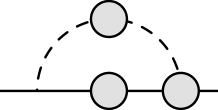
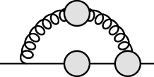
Figure 2: Feynman diagrams of the exact SD equations for the $t$ and $b$ quark propagators corresponding to Eqs.(11) and (12). $S_{0}^{-1}$ in the first term of the right-hand side stands for the tree-level inverse propagators, $iS_{0}^{-1}(p)|_{t,b}=\not{p}-\frac{y_{t,b}}{\sqrt{2}}\sigma_{h}$. The blobs include all possible quantum corrections in the present gauge-Higgs-Yukawa system.

II.2 The ladder truncation and gauge fixing

We apply the ladder approximation for QCD, such that the gauge-fermion-fermion vertex functions are taken to be of tree level:

$$\Gamma^{(3),\nu}_{\bar{t}At,a}(p,q)=\Gamma^{(3),\nu}_{\bar{b}Ab,a}(p,q)=-ig_{s}\gamma^{\nu}T_{a}.$$ (6)

The abelian-type Ward-Takahashi identity with this truncation constrains the fermion full propagators as Miransky:1994vk

$$iS_{t/b}^{-1}=A_{t/b}(-p^{2})\not{p}-B_{t/b}(-p^{2})\,,\qquad{\rm with}\qquad A_{t/b}(-p^{2})=1\,.$$ (7)

It is well-known that in the pure QCD case, this condition can be fulfilled by taking the Landau gauge: $\xi=0$. The present case is, however, more involved, which also includes the Yukawa and Higgs quartic interactions. First of all, we therefore examine the consistency of the Landau gauge choice for the present system to satisfy Eq.(7). As it will turn out right below, the extended ladder approximation with the bare propagators for both scalar and gauge fields in the Landau gauge is shown to be numerically consistent well with Eq.(7).

To prove this point, we take the tree-level propagators for the scalar and gauge fields as

$$\Delta_{\sigma}(k)=\frac{i}{k^{2}-3\lambda_{\phi}\sigma_{h}^{2}},$$ (8)

$$\Delta_{\pi_{i}}(k)=\frac{i}{k^{2}-\lambda_{\phi}\sigma_{h}^{2}},$$

$$\Delta_{g,\mu\nu}^{ab}(k)=\frac{-i\delta^{ab}}{k^{2}}\left(g_{\mu\nu}-(1-\xi)\frac{k_{\mu}k_{\nu}}{k^{2}}\right),$$

and all the relevant vertices to be bare ones:

$$\Gamma^{(3)}_{\bar{t}\sigma t}(p,q)=\frac{-iy_{t}}{\sqrt{2}},\quad\Gamma^{(3)}_{\bar{t}\pi_{3}t}(p,q)=\frac{-\gamma_{5}y_{t}}{\sqrt{2}},$$ (9)

$$\Gamma^{(3)}_{\bar{t}\pi_{1}b,R}(p,q)=\frac{-y_{b}P_{R}}{\sqrt{2}},\quad\Gamma^{(3)}_{\bar{t}\pi_{2}b,R}(p,q)=\frac{-iy_{b}P_{R}}{\sqrt{2}},$$

$$\Gamma^{(3)}_{\bar{t}\pi_{1}b,L}(p,q)=\frac{y_{t}P_{L}}{\sqrt{2}},\quad\Gamma^{(3)}_{\bar{t}\pi_{2}b,L}(p,q)=\frac{iy_{t}P_{L}}{\sqrt{2}},$$

$$\Gamma^{(3)}_{\bar{b}\sigma b}(p,q)=\frac{-iy_{b}}{\sqrt{2}},\quad\Gamma^{(3)}_{\bar{b}\pi_{3}b}(p,q)=\frac{\gamma_{5}y_{b}}{\sqrt{2}},$$ (10)

$$\Gamma^{(3)}_{\bar{b}\pi_{1}t,R}(p,q)=\frac{-y_{t}P_{R}}{\sqrt{2}},\quad\Gamma^{(3)}_{\bar{b}\pi_{2}t,R}(p,q)=\frac{iy_{t}P_{R}}{\sqrt{2}},$$

$$\Gamma^{(3)}_{\bar{b}\pi_{1}t,L}(p,q)=\frac{y_{b}P_{L}}{\sqrt{2}},\quad\Gamma^{(3)}_{\bar{b}\pi_{2}t,L}(p,q)=\frac{-iy_{b}P_{L}}{\sqrt{2}}.$$

With this prescription, after a tedious computation, the $A_{t/b}(p_{E}^{2})$ and $B_{t/b}(p_{E}^{2})$ functions (with $p_{E}^{2}\equiv-p^{2}$) take the form

$$B_{t}(p_{E}^{2})= \frac{y_{t}}{\sqrt{2}}\sigma_{h}+\int^{\Lambda^{2}}dq_{E}^{2}\mathcal{K}_{B_{t}}(p_{E}^{2},q_{E}^{2})\frac{q_{E}^{2}B_{t}(q_{E}^{2})}{A_{t}^{2}(q_{E}^{2})q_{E}^{2}+B_{t}^{2}(q_{E}^{2})}$$ (11)

$$+\frac{y_{t}y_{b}}{16\pi^{2}}\int^{\Lambda^{2}}dq_{E}^{2}K_{B}(p_{E}^{2},q_{E}^{2};\lambda_{\phi}\sigma_{h}^{2})\frac{q_{E}^{2}B_{b}(q_{E}^{2})}{A_{b}^{2}(q_{E}^{2})q_{E}^{2}+B_{b}^{2}(q_{E}^{2})},$$

$$A_{t}(p_{E}^{2})= 1+\int^{\Lambda^{2}}dq_{E}^{2}\mathcal{K}_{A_{t}}(p_{E}^{2},q_{E}^{2})\frac{A_{t}(q_{E}^{2})}{A_{t}^{2}(q_{E}^{2})q_{E}^{2}+B_{t}^{2}(q_{E}^{2})}$$

$$+\frac{{y_{t}}^{2}+{y_{b}}^{2}}{32\pi^{2}}\int^{\Lambda^{2}}dq_{E}^{2}K_{A}(p_{E}^{2},q_{E}^{2};\lambda_{\phi}\sigma_{h}^{2})\frac{A_{b}(q_{E}^{2})}{A_{b}^{2}(q_{E}^{2})q_{E}^{2}+B_{b}^{2}(q_{E}^{2})},$$

$$B_{b}(p_{E}^{2})= \frac{y_{b}}{\sqrt{2}}\sigma_{h}+\int^{\Lambda^{2}}dq_{E}^{2}\mathcal{K}_{B_{b}}(p_{E}^{2},q_{E}^{2})\frac{q_{E}^{2}B_{t}(q_{E}^{2})}{A_{b}^{2}(q_{E}^{2})q_{E}^{2}+B_{b}^{2}(q_{E}^{2})}$$ (12)

$$+\frac{y_{t}y_{b}}{16\pi^{2}}\int^{\Lambda^{2}}dq_{E}^{2}K_{B}(p_{E}^{2},q_{E}^{2};\lambda_{\phi}\sigma_{h}^{2})\frac{q_{E}^{2}B_{t}(q_{E}^{2})}{A_{t}^{2}(q_{E}^{2})q_{E}^{2}+B_{t}^{2}(q_{E}^{2})},$$

$$A_{b}(p_{E}^{2})= 1+\int^{\Lambda^{2}}dq_{E}^{2}\mathcal{K}_{A_{b}}(p_{E}^{2},q_{E}^{2})\frac{A_{b}(q_{E}^{2})}{A_{b}^{2}(q_{E}^{2})q_{E}^{2}+B_{b}^{2}(q_{E}^{2})}$$

$$+\frac{{y_{t}}^{2}+{y_{b}}^{2}}{32\pi^{2}}\int^{\Lambda^{2}}dq_{E}^{2}K_{A}(p_{E}^{2},q_{E}^{2};\lambda_{\phi}\sigma_{h}^{2})\frac{A_{t}(q_{E}^{2})}{A_{t}^{2}(q_{E}^{2})q_{E}^{2}+B_{t}^{2}(q_{E}^{2})}\,,$$

where the integral kernels are given by

$$\mathcal{K}_{B_{t}}(x,y)=(1+\xi/3)\frac{3{g_{s}}^{2}C_{F}}{16\pi^{2}}K_{B}(x,y;0)+\frac{{y_{t}}^{2}}{32\pi^{2}}\left[K_{B}(x,y;\lambda_{\phi}\sigma_{h}^{2})-K_{B}(x,y;3\lambda_{\phi}\sigma_{h}^{2})\right],$$ (13)

$$\mathcal{K}_{A_{t}}(x,y)=\frac{y}{x}\left\{\xi\frac{4{g_{s}}^{2}C_{F}}{16\pi^{2}}K_{A}(x,y;0)+\frac{{y_{t}}^{2}}{32\pi^{2}}\left[K_{A}(x,y;3\lambda_{\phi}\sigma_{h}^{2})+K_{A}(x,y;\lambda_{\phi}\sigma_{h}^{2})\right]\right\}$$

and

$$K_{B}(x,y;M^{2}) =\frac{2}{x+y+M^{2}+\sqrt{(x+y+M^{2})^{2}-4xy}},$$ (14)

$$K_{A}(x,y;M^{2}) =\frac{2xy}{\left[x+y+M^{2}+\sqrt{(x+y+M^{2})^{2}-4xy}\right]^{2}},$$

with $C_{F}=T^{a}T_{a}=({N_{c}}^{2}-1)/(2N_{c})=4/3$. We have regularized the momentum integrals by the momentum cutoff $\Lambda$. This cutoff scale $\Lambda$ acts as the ultraviolet regulator in the LSD equations, and is identified as infrared scales for the perturbative renormalization group running. This is in the later section to coincide with a matching scale between the quark-meson model-like description at low energy and the present gauge-Higgs-Yukawa system.

Figure 3 shows the momentum dependence of $A_{t/b}(p_{E}^{2})$ with $\xi=0$ in the regime that is what is called the nonperturbative regime, relevant to the present study with the input parameters to be addressed in details in the later section. We find $A_{t/b}(p_{E}^{2})\simeq 1$ in the target momentum range, thus the present extended ladder truncation works with $A_{t/b}=1$ in the Landau gauge $\xi=0$, in a way similar to the literature Kondo:1993ty in the $U(2)_{L}\times U(2)_{R}$ invariant limit.

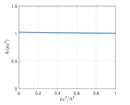
Figure 3: The Euclidean momentum dependence of $A\equiv A_{t/b}$. The parameter setup has been taken as $y_{t}\simeq 2.6$, $g_{s}\simeq 3.1$, $y_{b}\simeq 0.063$, and $\lambda_{\phi}\simeq 0.93$ at the cutoff scale $\Lambda\simeq 234$ MeV below which the nonperturbative regime in the chiral broken phase governs.

III The CJT potential in the ladder approximation and phase structure of the gauge-Higgs-Yukawa system

In this section, we work on the CJT formalism Cornwall:1974vz to get the CJT potential at the two-loop level in the ladder approximation and reproduce the LSD equations, Eqs.(11), (12), and (5). This CJT formalism also makes a preliminary setup to facilitate the matching procedure linked to a quark-meson model-like description in the later section. We then discuss the phase structure of the present gauge-Higgs-Yukawa system on the model parameter space along with the SM benchmark point, as referred to in Figs. 1 and 3. The SM quark masses at the benchmark infrared scale ($\Lambda\simeq 234$ MeV) are also computed.

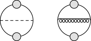
Figure 4: The two types of diagrams contributing to $V_{2}$ in Eq.(15) in the ladder approximation, where the solid curve represents quark propagators, the dashed one the scalars, and the wavy curve the one for the gluons.

III.1 The CJT effective potential

We begin by writing the CJT effective potential in the presently applied ladder approximation up to the two-loop level,

$$V_{\rm eff}[\sigma_{h},S_{t},S_{b}]=V_{0}(\sigma_{h})+V_{\text{scalar}}^{\text{1-loop}}(\sigma_{h},\Delta_{\sigma,\pi_{i}})+V_{\text{quarks}}^{\text{1-loop}}(S_{t,b})+V_{\text{gauge}}^{\text{1-loop}}(\Delta_{g})+V_{2}(\phi_{c},\Delta_{\sigma,\pi_{i}},S_{t,b},\Delta_{g})+\text{const.},$$ (15)

where $V_{0}(\sigma_{h})=\frac{\lambda_{\phi}}{4}\sigma_{h}^{4}$ is the tree-level potential, and

$$V_{\text{scalar}}^{\text{1-loop}}(\sigma_{h},\Delta_{\sigma/\pi_{i}}) =-\frac{i}{2}\text{tr}\,\ln{i\Delta_{\sigma_{h}/\pi_{i}}^{-1}}\,,$$

$$V_{\text{quarks}}^{\text{1-loop}}(S_{t/b}) =i\,\text{tr}\,\ln{iS^{-1}_{t/b}}+i\,\text{tr}\left[S^{-1}_{0t/b}(\sigma_{h})S_{t/b}\right]\,,$$

$$V_{\text{gauge}}^{\text{1-loop}}(\Delta_{g}) =-\frac{i}{2}\text{tr}\,\ln{i\Delta_{g}^{-1}}\,,$$ (16)

with the inverse-tree propagators for $t$ and $b$ quarks defined as $S_{0t/b}^{-1}=\not{p}-\frac{y_{t/b}}{\sqrt{2}}\sigma_{h}$. The $V_{2}$ term denotes the contribution from diagrams at the two-loop level, which in the present ladder approximation includes the graphs depicted in Fig. 4. In the first line of Eq.(16), $\Delta_{\sigma/\pi_{i}}^{-1}$ do not take into account the nonperturbative effects on the scalar two-point functions, i.e., $V_{\text{scalar}}^{\text{1-loop}}(\sigma_{h},\Delta_{\sigma/\pi_{i}})$ should be the one-particle irreducible potential for $\sigma$ and $\pi_{i}$ fields, which depends only on the Higgs VEV. Taking into account $A_{t/b}=1$ in the Landau gauge ($\xi=0$), one can compute $V_{\rm eff}$ to reach the form

$$V_{\text{eff}}[\sigma_{h},B_{t},B_{b}]= \frac{\lambda_{\phi}}{4}{\sigma_{h}}^{4}+\frac{1}{32\pi^{2}}\int^{\Lambda^{2}}dk_{E}^{2}\,k_{E}^{2}\ln{\frac{k_{E}^{2}+3\lambda_{\phi}\sigma_{h}^{2}}{k_{E}^{2}}}+\frac{3}{32\pi^{2}}\int^{\Lambda^{2}}dk_{E}^{2}\,k_{E}^{2}\ln{\frac{k_{E}^{2}+\lambda_{\phi}\sigma_{h}^{2}}{k_{E}^{2}}}$$

$$+\frac{N_{c}}{4\pi^{2}}\int^{\Lambda^{2}}dp_{E}^{2}\,p_{E}^{2}\frac{B_{t}^{2}(p_{E}^{2})-y_{t}\sigma_{h}{B_{t}}(p_{E}^{2})/\sqrt{2}}{p_{E}^{2}+B_{t}^{2}(p_{E}^{2})}$$

$$+\frac{N_{c}}{4\pi^{2}}\int^{\Lambda^{2}}dp_{E}^{2}\,p_{E}^{2}\frac{B_{b}^{2}(p_{E}^{2})-y_{b}\sigma_{h}{B_{b}}(p_{E}^{2})/\sqrt{2}}{p_{E}^{2}+B_{b}^{2}(p_{E}^{2})}\,.$$

The stationary conditions with respect to $B_{t}$ and $B_{b}$ respectively reproduce the SD equations for $B_{t}$ and $B_{b}$ in Eqs.(11) and Eq.(12) with the present ladder approximation prescribed.

The tadpole condition for the Higgs VEV in Eq.(5) is also derived with respect to $\sigma_{h}$, which, neglecting the small $b$ quark contribution, takes the same form as in Eq.(5). The three-point function in the left-hand side of Eq.(5) can be decomposed as

$$\braket{\sigma(\sigma^{2}+\vec{\pi}^{2})}=\braket{\sigma}^{3}+3\braket{\sigma}\braket{\sigma\sigma}_{\text{conn.}}+\braket{\sigma}\braket{\pi_{i}\pi_{i}}_{\text{conn.}}+\braket{\sigma(\sigma^{2}+\pi_{i}^{2})}_{\text{conn.}}\,,$$ (17)

where the subscript “conn.” stands for the amplitude constructed from connected diagrams. The present ladder approximation the right-hand side of Eq.(17) into only the first two terms with the bare bosonic propagators, so that we have

$$\braket{\sigma(\sigma^{2}+\vec{\pi}^{2})} =\lambda_{\phi}\sigma_{h}^{3}+\lambda_{\phi}\sigma_{h}\int\frac{d^{4}q}{(2\pi)^{4}}\left(\frac{3i}{q^{2}-3\lambda_{\phi}\sigma_{h}^{2}}+\frac{3i}{q^{2}-\lambda_{\phi}\sigma_{h}^{2}}\right)$$ (18)

$$=\lambda_{\phi}\sigma_{h}^{3}+\frac{3\lambda_{\phi}\sigma_{h}}{16\pi^{2}}\left(2\Lambda^{2}-3\lambda_{\phi}\sigma_{h}^{2}\ln{\frac{\Lambda^{2}-3\lambda_{\phi}\sigma_{h}^{2}}{3\lambda_{\phi}\sigma_{h}^{2}}}-\lambda_{\phi}\sigma_{h}^{2}\ln{\frac{\Lambda^{2}-\lambda_{\phi}\sigma_{h}^{2}}{\lambda_{\phi}\sigma_{h}^{2}}}\right).$$

The right hand side of Eq.(5), i.e., the top quark condensate $(-\frac{y_{t}}{\sqrt{2}}\langle\bar{t}t\rangle)$, is similarly simplified, in the present ladder approximation, to

$$-\frac{y_{t}}{\sqrt{2}}\langle\bar{t}t\rangle =\frac{y_{t}N_{c}}{\sqrt{2}}\int\frac{d^{4}q}{(2\pi)^{4}}\text{tr}S_{t}(q)=\frac{y_{t}N_{c}}{4\sqrt{2}\pi^{2}}\int^{\Lambda^{2}}dp_{E}^{2}\frac{p_{E}^{2}B_{t}(p_{E}^{2})}{p_{E}^{2}+{B_{t}^{2}(p_{E}^{2})}}\,.$$ (19)

The current quark masses are generated by the Higgs VEV $\sigma_{h}$ as the solution of Eq.(5), coupled with the SD equations for $B_{t}$ and $B_{b}$ in Eqs.(11) and (12), to be

$$m_{q}=\frac{y_{q}}{\sqrt{2}}\sigma_{h},$$ (20)

for $q$-quark. The full masses for $t$ and $b$ quarks are defined as

$$m_{t/b,full}=B_{t/b}(p^{2}_{E}=m_{t/b,full}^{2})\,.$$ (21)

III.2 The phase structure and implication to SM quark masses

Numerically solving the coupled LSD equations, Eqs.(11), (11), and (5), in Fig. 5 we show a phase diagram in the space spanned by the dynamical top mass normalized to the cutoff $m_{t,full}/\Lambda$, $y_{t}$, and $\lambda_{\phi}$, with $g_{s}=y_{t}$ and $y_{b}=0.5y_{t}$. The critical line has been observed on the $(y_{t},\lambda_{\phi})$ plane placed by $m_{t,full}=0$. In the limit where $\lambda_{\phi}\to 0$, $m_{t,full}$ goes divergent, which reflects the non-renormalizability of the Yukawa theory in the absence of the scalar quartic coupling.

Here we have several remarks.

• The bare parameter setup on $g_{s}=y_{t}$ well models the infrared feature of the renormalization group running in the SM as seen from Fig. 1, when the cutoff $\Lambda$ for the SD equations matches with a strong coupling scale of $\alpha_{s}$, $\alpha_{s}(\Lambda)\sim\pi$.

• Though the input isospin breaking by $y_{b}=0.5y_{t}$ is too small to be realistic, the generic feature of the phase diagram does not substantially alter for smaller $y_{b}$.

• The chiral symmetric phase is still observed even with nonzero $\lambda_{\phi}$ and $y_{t}$ as long as $y_{t}\lesssim 1$, because the tadpole of the Higgs is generated via the top quark condensate following the SD Eq.(5).

• In the strong QED limit where $y_{t}=y_{b}=0$ and $\lambda_{\phi}\to\infty$ (i.e. the decoupling limit of the Higgs), we have observed the well-known critical coupling $g_{s}^{\rm cr}=\pi$ ($\alpha_{s}=\pi/(3C_{F})=\pi/4)$) Miransky:1994vk .

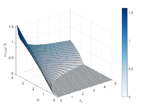
Figure 5: A mock-up phase diagram on $m_{t,full}/\Lambda$, $y_{t}$, and $\lambda_{\phi}$, with $g_{s}=y_{t}$ and $y_{b}=0.5y_{t}$.

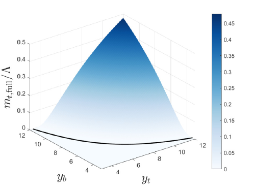
Figure 6: The phase diagram on $m_{t,full}/\Lambda$, $y_{t}$, and $y_{b}$, with $g_{s}=\lambda_{\phi}=0$. The critical line separating the chiral symmetric and broken phases is given as $y_{t}y_{b}=4\pi^{2}$.

In the Yukawa-theory limit with the massless scalars, we have found a critical line $y_{t}y_{b}=4\pi^{2}$ as shown in Fig. 6. The seemingly dominated $y_{t}^{2}$ terms in the LSD equation for $B_{t}$ in Eq.(11) are actually canceled in the kernel function ${\cal K}_{B_{t}}$ in Eq.(14) (with $\xi=0$). This feature is still approximately operative even with the massive scalar exchange contributions: ${\cal K}_{B_{t}}(x,y;m^{2})\simeq{\cal K}_{B_{t}}(x,y;3m^{2})$ as long as $m/\Lambda\ll 1$. This is essentially due to an accidental $U(1)$ axial symmetry between $\sigma$ and $\pi^{3}$ exchanges (repulsive and attractive channels): that is, $U(1)_{A}\equiv U(1)_{L,3}\times U(1)_{R,3}$, which is associated with the chiral rotation with respect to the third component of the Pauli matrix $\tau_{3}$ and transforms $\phi^{0}$ and the quark doublet field $q$ in the Yukawa terms, in Eq.(1), as

$$\phi^{0}\rightarrow e^{-i\theta}\phi^{0}\quad\text{and}\quad q\rightarrow e^{i\frac{\theta}{2}\gamma_{5}\tau_{3}}q\,,$$ (22)

making the coupling strengths of $\bar{q}\sigma q$ and $\bar{q}\pi_{3}q$ identical to each other.

Thus, the strong top Yukawa coupling $y_{t}$ cannot solely develop the critical line or does not dominantly generate the chiral broken phase, or the top quark condensate. Therefore, the dynamical chiral symmetry in the present gauge-Higgs-Yukawa system is essentially triggered by the ladder QCD (i.e. strong QED), and the top flavor characteristics on the top-quark full mass $m_{t,full}$ is provided only through the overall top Yukawa coupling: $m_{t,full}$ still lies in the QCD scale $={\cal O}$(100) MeV. This conclusion favors the description of almost massless six-flavor QCD when the QCD phase transition is addressed, which is to be clarified right below.

Figure 7 shows the current quark masses as a function of $\Lambda$, which arise from the Higgs tadpole contribution in Eq.(23) together with the LSD solutions. The selected range of $\Lambda$ includes a reference point $\Lambda=234$ MeV where we have $g_{s}(\Lambda)\simeq 3.1\sim\pi$, i.e., close to the critical coupling in strong QED, which corresponds to a boundary between the perturbative nonperturbative coupling regimes as quoted in Fig. 3: at $\Lambda=234$ MeV the SM perturbative two-loop running, with the EW scale inputs as in Fig. 1, yields $y_{t}\simeq 2.6$, $g_{s}\simeq 3.1$, $y_{b}\simeq 0.063$, and $\lambda_{\phi}\simeq 0.93$. Figure 3 indeed implies that at around the reference point $\Lambda=234$ MeV, we have current quark masses for the SM heavier three quarks (the Higgs tadpole contribution in Eq.(23)),

$$m_{t}(\Lambda=234\,{\rm MeV}) \simeq 140\,{\rm MeV}\,,$$

$$m_{b}(\Lambda=234\,{\rm MeV}) \simeq 3.5\,{\rm MeV}\,,$$

$$m_{c}(\Lambda=234\,{\rm MeV}) \simeq 0.94\,{\rm MeV}\,.$$ (23)

In addition, the top and bottom quarks get the pure ladder QCD and Yukawa contributions due to the top condensation. At the same reference point of $\Lambda$, we find the full masses for $t$ and $b$ quarks,

$$m_{t,full}(\Lambda=234\,{\rm MeV}) \simeq 175\,{\rm MeV}\,,$$

$$m_{b,full}(\Lambda=234\,{\rm MeV}) \simeq 12\,{\rm MeV}\,.$$ (24)

Thus all the six quarks can be light enough in the typical QCD phase transition epoch at around the temperature $\sim 100-200$ MeV.

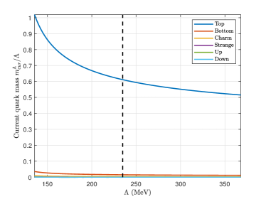
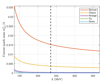
Figure 7: The plots of current quark masses versus $\Lambda$ including a reference point $\Lambda=234$ MeV, at which we have $g_{s}(\Lambda)\simeq 3.1\sim\pi$, i.e., close to the critical coupling in strong QED, following the SM perturbative renormalization evolution as in Fig. 3. The panel (b) excludes the top quark, while the panel (a) includes it.

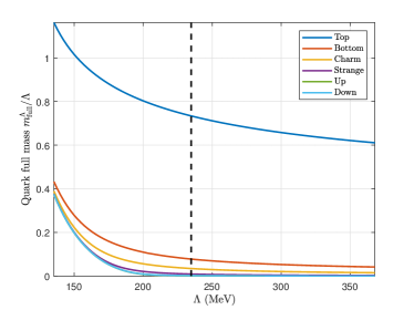
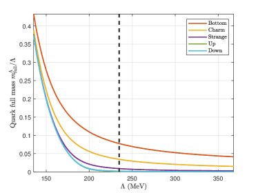
Figure 8: Quark full masses as a function of $\Lambda$ in the same range as in Fig. 7.

IV Cosmological implication of the top quark condensation in supercooled EW phase transition

Since the dynamically generated top condensate couples to the SM Higgs, the supercooled EW phase transition should get a significant correlation with the thermal evolution of the top condensate. In this section, we address this issue by employing a quark-meson model in the large $N_{c}$ limit. namely, the mean-field approximation for the Higgs and QCD meson fields. We fix the model parameters by matching them to the LSD results with the matching scale set at $\Lambda=234$ MeV, which is identified as the LSD cutoff scale as has been done in the previous section. We then discuss the cosmological phase transition arising from the evidence of the top quark condensation and its cosmological consequences such as the GW production.

IV.1 Quark meson model for the top-Higgs sector

Figure 9: The Feynman graph generating the $\sigma_{t}$ - $\sigma_{h}$ mixing. The blob and (internal) top loop lines include the nonperturbative ladder-type contributions as has been discussed in Sec.III.

We consider a quark-meson model-like model for the low-energy effective description for the present gauge-Higgs-Yukawa system at the matching scale $\Lambda$. Since the correlation with the SM Higgs arising only through the Yukawa couplings to quarks, the mean-field associated with only the top quark condensate becomes significant. The model Lagrangian is thus constructed from the scale-invariant SM Higgs sector (only with neutral scalars) coupled to the top quark:

$$\mathcal{L}_{\text{QMM}} =\bar{t}i\not{\partial}t-g\,\bar{t}_{L}M_{\bar{t}t}t_{R}-y_{t}\,\bar{t}_{L}M_{h}t_{R}+\text{h.c.}$$

$$+\partial_{\mu}M_{\bar{t}t}^{\dagger}\partial^{\mu}M_{\bar{t}t}+\partial_{\mu}M_{h}^{\dagger}\partial^{\mu}M_{h}-V_{\rm QMM}\,,$$

$$V_{\rm QMM} =\lambda_{\phi}\left(M_{h}^{\dagger}M_{h}\right)^{2}-g_{m}(M_{h}^{\dagger}M_{\bar{t}t}+{\rm h.c.})+V(M_{\bar{t}t})\,,$$ (25)

where $M_{\bar{t}t}=(\sigma_{t}+i\pi_{t})/\sqrt{2}$ for the $\bar{t}t$ scalar meson, i.e., topponium, and $M_{h}=(\sigma_{h}+i\pi_{h})/\sqrt{2}$ for the neutral Higgs scalar fields in the SM. Here several comments are in order:

• The $g_{m}$ coupling term denotes the mixing between the topponium and the SM Higgs mean fields, $-g_{m}\langle\sigma_{h}\rangle\langle\sigma_{t}\rangle$, which corresponds to the disconnected graph contribution in the ladder approximation. See Fig. 9 for the typical Feyman graph. The figure also displays a squared blob, which denotes the Bethe-Salpeter amplitude to describe the dynamical $\sigma_{t}$ - $t$ - $t$ vertex, including not merely the static potential terms, but also the momentum dependence. The latter type of quantum corrections are discarded in the current ladder approximation. The momentum dependence will not give any significance on the static potential analysis aiming at discussion on the thermal phase transition, which might, however, be the issue when the dynamic cosmological phase transition is addressed. We will come back to this point later in the Summary and Discussion section.

• In addition to the tadpole term, in Eq.(25) the top Yukawa coupling to $M_{h}$ has been taken into account, so that the top-quark full mass contributions are shared by those two terms due to the presence of the dynamical Higgs field. This is in contrast to the case of the ordinary QCD quark-meson model which includes the current quark mass effect in the tadpole term and the dynamical mass part in the Yukawa term.

• One can also see that the second derivative of the CJT potential with respect to $\sigma_{h}$ in Eq.(III.1) vanishes, which implies no Higgs portal coupling to $\sigma_{t}$, such as $|M_{h}|^{2}|M_{\bar{t}t}|^{2}$, hence the $g_{m}$ coupling is the unique way to allow the mixing of $M_{\bar{t}t}$ with $M_{h}$ up to operators smaller than dimension four.

• The topponium VEV at the vacuum, $\braket{\sigma_{t}}$, is set by the topped pion decay constant $f_{t}$, which we nonperturbatively compute by using the Pagels-Stokar formula Pagels:1979hd with the solution of the coupled LSD equations (Eqs.(11), (12), and (5)) as

  $$f_{t}^{2}=\frac{N_{c}}{4\pi^{2}}\int^{\Lambda^{2}}dp_{E}^{2}\cdot p_{E}^{2}\frac{B_{t}^{2}(p_{E}^{2})-\frac{p_{E}^{2}}{4}\frac{d}{dp_{E}^{2}}B_{t}^{2}(p_{E}^{2})}{(p_{E}^{2}+B_{t}^{2}(p_{E}^{2}))^{2}}\,.$$ (26)

  The numerical estimate gives $f_{t}/\Lambda\simeq 0.091$ and for Higgs VEV $\sigma_{h}/\Lambda\simeq 0.34$ at $\Lambda=234$ MeV with the same inputs as in Eqs.(23) and (24).

Besides, we have the potential term for $M_{\bar{t}t}$ in Eq.(25). Taking $\pi_{t}=0$ via the U(1) axial transformation, the mesonic potential can be written as a function of only $\sigma_{t}$. At this point, a simple-minded parametrization of the potential is of the Ginzburg-Landau polynomial form,

$$V(M_{\bar{t}t})\Bigg{|}_{\rm GL}=\mu^{2}\sigma_{t}^{2}+\lambda\sigma_{t}^{2}\,.$$ (27)

The presence of the mass term $\mu^{2}$ would reflect the hard scale breaking at the deeper infrared regime of QCD, simply following the perturbative running of the gauge coupling (as seen also from Fig. 1). Still, we could have another possibility featuring the deeply infrared QCD nature: in a recent nonperturbative analysis based on the functional renormalization group, like in the literature Deur:2023dzc , the QCD gauge coupling might possess a nontrivial infrared fixed point, which implies an almost scale invariance (to be eventually broken by the dynamical chiral symmetry breaking, though) . From this perspective, we might also consider the Coleman-Weinberg type Coleman:1973jx ,

$$V(M_{\bar{t}t})\Bigg{|}_{\rm CW}=\lambda\sigma_{t}^{4}\left[a+b\ln\left(\frac{\sigma_{t}}{f_{t}}\right)\right]\,.$$ (28)

Taking into account both two possibilities, thus we model the form of $V(M_{\bar{t}t})$ as

$$V_{M_{\bar{t}t}}=\lambda_{D}\,\left(\frac{\sigma_{t}}{f_{t}}\right)^{4-\gamma_{D}}{f_{t}}^{4}+\lambda\left(\frac{\sigma_{t}}{f_{t}}\right)^{4}{f_{t}}^{4}.$$ (29)

Here we have introduced an anomalous dimension parameter $\gamma_{D}$ associated with the scale anomaly, which can be fixed by solving the underlying theory. In the present study, we take it as a free parameter and consider $\gamma_{D}$ in a range of $0<\gamma_{D}\leq 2$. The $\lambda_{D}$ term thus plays a role of interplay between the Ginzburg-Landau and almost scale-invariant description. When $\gamma_{D}=2$ the $\lambda_{D}$ term is reduced to the normal quadratic mass term as in Eq.(27), while for $\gamma_{D}\simeq 0$ it provides a logarithmic potential term like $\lambda_{D}\,\gamma_{D}\sigma_{t}^{4}\log(\sigma_{t}/f_{t})$:

$$V(M_{\bar{t}t})\Bigg{|}_{\gamma_{D}\simeq 0} =\sigma_{t}^{4}\left[(\lambda+\lambda_{D})-\lambda_{D}\gamma_{D}\ln\left(\frac{\sigma_{t}}{f_{t}}\right)+\mathcal{O}(\gamma_{D}^{2})\right]\equiv V(M_{\bar{t}t})\Bigg{|}_{\rm CW}\quad{\rm in}\quad{\rm Eq.(\ref{CW-type})}\,.$$ (30)

We fix the vacuum feature of the model including the Higgs VEV $\langle\sigma_{h}\rangle$, the topponium VEV $\langle\sigma_{t}\rangle=f_{t}$, and the potential energy i.e., the scale anomaly, by matching with the nonperturbative results associated with the CJT effective potential in Eq.(III.1). First, the stationary condition for the potential terms, together with the LSD solutions to $\langle\sigma_{t}\rangle=f_{t}$ (Eq.(26)) and $\langle\sigma_{h}\rangle$ (Eq.(5)), constrain $\lambda_{D}$, $\gamma_{D}$, and $g_{m}$, as follows:

$$\left.\frac{\partial V}{\partial\sigma_{h}}\right|_{\text{vacuum}}=\lambda_{\phi}\sigma_{h}^{3}-g_{m}f_{t}=0;$$ (31)

$$\left.\frac{\partial V}{\partial\sigma_{t}}\right|_{\text{vacuum}}=\lambda_{D}(4-\gamma_{D}){f_{t}}^{3}+4\lambda{f_{t}}^{3}-g_{m}\sigma_{h}=0.$$

Then, matching with the vacuum energy gives a further constraint like

$$V_{\rm CJT}\Bigg{|}_{\rm vacuum}\equiv V_{QMM}\Bigg{|}_{\rm vacuum}=\frac{1}{4}\left(\lambda_{D}{f_{t}}^{4}-2g_{m}\langle\sigma_{h}\rangle f_{t}\right)\,.$$ (32)

Though the $g$ coupling between quark and meson is at this point just free parameter, referring to the LSD results may fix it via the constituent quark mass in the following two ways (I and II)

$$g|_{I}=\left(m_{t,full}-\frac{y_{t}}{\sqrt{2}}\langle\sigma_{h}\rangle\right)/f_{t},$$ (33)

$$g|_{II}=m_{t,full}/f_{t}.$$

In the former case ($g|_{I}$), $M_{\bar{t}t}$ couples to the top quark pair only via the dynamical mass of the top quark, while keeping the tadpole term coupled to the Higgs mean field. The latter case ($g|_{II}$) implies that the top quark pair still couples to $M_{\bar{t}t}$ also through the current mass, so that there are two current mass contributions to the model along with the tadpole term. The LSD result at the reference point $\Lambda=234$ MeV gives

$$g|_{I} \simeq 1.3\,,$$

$$g|_{II} \simeq 8.0\,.$$ (34)

Thus the model parameters can completely be fixed once $\gamma_{D}$ is given for $0<\gamma_{D}\leq 2$. Table 1 gives the model parameter sets fixed by matching with the present LSD analysis as described above.

$\gamma_{D}$	2		0.5		0.1
$g$	1.3	8.0	1.3	8.0	1.3	8.0
$g_{m}/\Lambda^{2}$	0.39
$\lambda$	50		89		299
$\lambda_{D}$	-13		-52		-262

Table 1: The parameter setting of the present quark-meson model fixed by the matching with the LSD analysis at $\Lambda=234$ MeV, given a value of $\gamma_{D}$ in a range of $0<\gamma_{D}\leq 2$.

IV.2 Thermal phase transition

We incorporate the thermal loop corrections arising from the top-Yukawa interaction at the one-loop level of the quark-meson model in Eq.(25), based on the imaginary time formalism, to derive the thermodynamic potential ($\Omega(\sigma_{t},\sigma_{h})$) for the mean fields $\sigma_{t}$ and $\sigma_{h}$. The top loop corrections to the vacuum part are not included in the thermodynamic potential, instead, which involves nonperturbative corrections from the LSD analysis in the tree level as has been discussed above.

Figure 10 shows the temperature ($T$) dependence (normalized to $\Lambda=234$ MeV) of $\sigma_{t}$ and $\sigma_{h}$ in the case of $\gamma_{D}=2$ with $g|_{I}$ and $g|_{II}$ in Eq.(34). For larger $g$, the phase transition goes like the type of the first-order with the critical temperature $T_{c}\simeq 65$ MeV, while for smaller $g$, it tends to be changed to crossover with the pseudocritical temperature (defined as the inflection point of the order parameter) $T_{\rm pc}\simeq 80$ MeV, which holds approximately for both $\sigma_{t}$ and $\sigma_{h}$. We have checked that this trend does not substantially change for smaller $\gamma_{D}$. The first-order phase transition has been undergone due to the emergence of the thermal potential barrier between the false and true vacua, which has been created along a hybrid direction involving two nonzero $\sigma_{t}$ and $\sigma_{h}$, as plotted in Fig. 11. This is the characteristic consequence of the presence of the top quark condensate in the thermal history.

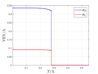
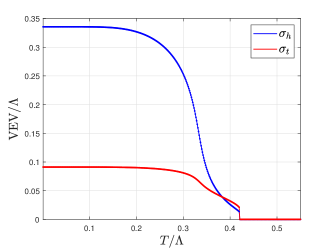
Figure 10: The temperature dependence of $\sigma_{t}$ and $\sigma_{h}$ in the case of $\gamma_{D}=2$ for (a) $g|_{II}\simeq 8.0$ and (b) $g|_{I}\simeq 1.3$.

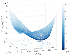
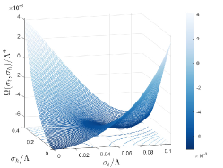
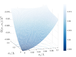
Figure 11: The thermodynamic potentials as a function of $\sigma_{t}$ and $\sigma_{h}$ for $\gamma_{D}=2$ with $g|_{II}\simeq 8.0$ around the first order phase transition point. The panel (a) corresponds to the case when $T=0.5T_{c}$; (b) $T=1.0T_{c}$; (c) $T=1.5T_{c}$, where $T_{c}\simeq 65$ MeV for the matching scale $\Lambda=234$ MeV.

IV.3 Cosmological phase transition

The first-order phase transition in the hybrid $\sigma_{t}$-$\sigma_{h}$ system at around $T_{c}\simeq 65$ MeV would be supercooled in the universe to produce the bubble nucleation and percolation. We discuss this supercooling in terms of the false vacuum decay and evaluate the false vacuum decay rate approximately as Linde:1981zj

$$\Gamma\simeq T^{4}\left(\frac{\mathcal{S}_{3}}{2\pi T}\right)^{\frac{3}{2}}\exp{\left(-\frac{\mathcal{S}_{3}}{T}\right)}\,,$$ (35)

where the $\mathcal{S}_{3}=\mathcal{S}_{3}[\phi_{\text{b}}(r)]$ is the three-dimensional ${\cal O}(3)$ symmetric Euclidean action ,

$$\mathcal{S}_{3}=\int dr\,(4\pi r^{2})\left[\frac{1}{2}\left(\frac{d\vec{\sigma}}{dr}+\Omega(\vec{\sigma},T)\right)\right]\,,$$ (36)

with a set of the bounce solutions $\vec{\sigma}(r)=(\sigma_{t},\sigma_{h})^{T}$. The bounce solutions are given by solving the stationary condition of the action:

$$\frac{d^{2}\vec{\sigma}}{dr^{2}}+\frac{2}{r}\frac{d\vec{\sigma}}{dr}=\nabla_{\sigma}\Omega(\vec{\sigma},r)\,,$$ (37)

with the boundary conditions

$$\left.\frac{d\vec{\sigma}}{dr}\right|_{r=0}=0,$$ (38)

$$\left.\vec{\sigma}\right|_{r\rightarrow\infty}=0.$$

To get the multi-field bounce solutions, we have used the numerical source pack CosmoTransitions Wainwright:2011kj .

Then the nucleation temperature $T_{n}$ can be determined by

$$\frac{\Gamma(T_{n})}{H^{4}(T_{n})}\sim 1.$$ (39)

where the Hubble parameter is parametrized as

$$H^{2}(T)=\frac{\rho_{\text{rad}}(T)+\rho_{\text{vac}}(T)}{{3M_{\text{Pl}}}^{2}}\simeq\frac{1}{{3M_{\text{Pl}}}^{2}}\left(\frac{\pi^{2}}{30}g_{*}(T_{i})T_{i}^{4}+\Delta V\right)\,,$$ (40)

with $\Delta V$ being the vacuum energy density difference between the false vacuum and the true vacuum. Here $g_{*}(T)$ denotes the effective degrees of freedom at $T$, and $M_{\rm pl}$ is the reduced Planck scale $\simeq 1.2\times 10^{18}$ GeV. We have also taken into account the dark-sector induced potential density, which is parametrized by a dark thermal density with $T_{i}$ as done in the literature Sagunski:2023ynd . This term can be turned off or on depending on whether the electroweak/dark sector phase transition is triggered before the hybrid $\sigma_{t}$ - $\sigma_{h}$ phase transition takes place, or not.

We also evaluate the percolation temperature $T_{p}$ via the probability still staying in the false vacuum Guth:1979bh ; Guth:1981uk , $P=e^{-I(T)}$, where the exponent function is available in the literature Ellis:2018mja ; Sagunski:2023ynd We define $T_{p}$ at which $I(T_{p})=0.34$ yielding $P\simeq 0.7$ Guth:1979bh ; Guth:1981uk .

IV.4 GW signals

We now discuss the GW signals produced from the supercooled QCD -EW phase transitions induced from the topponium - Higgs correlation. We evaluate the two characteristic signal parameters, $\alpha$ and $\beta$. The normalized latent heat $\alpha$ is defined as

$$\alpha(T_{p})\equiv\frac{1}{\rho_{\text{rad}}}\left(\rho_{\rm rad}(T_{i})+\Delta V-T\frac{d(\Delta V)}{dT}\right)_{T=T_{p}}\,,$$ (41)

where $\rho_{\rm rad}(T_{i})=\frac{\pi^{2}}{30}g_{*}(T_{i})T_{i}^{4}$, which is removed depending on the assumed dark-sector supercooling scenario Sagunski:2023ynd . The other parameter $\beta$ measures the inverse duration of the phase transition, and the normalized one ($\beta$) is defined as

$$\tilde{\beta}\equiv\frac{\beta}{H(T_{p})}=T_{p}\frac{d}{dT}\left(\frac{\mathcal{S}_{3}(T)}{T}\right).$$ (42)

Given the signal parameters as above, we calculate the gravitational wave spectra sourced from the bubble collision. The power spectrum is given by Brdar:2018num

$$\Omega_{\text{coll}}h^{2}=e^{-4N_{e}}\left(\frac{\rho_{p}}{\rho_{r}}\right)\times 1.67\times 10^{-5}\left(\frac{\beta}{H(T_{p})}\right)^{-2}\left(\frac{\kappa_{\text{coll}}\alpha}{1+\alpha}\right)^{2}\left(\frac{100}{g_{*}}\right)^{1/3}\left(\frac{0.11{v_{w}}^{3}}{0.42+{v_{w}}^{2}}\right)\frac{3.8(f/f_{\text{coll}})^{2.8}}{1+2.8(f/f_{\text{coll}})^{3.8}},$$ (43)

where $\kappa_{\text{coll}}$ characterizes the energy transfer between the vacuum energy and the kinetic energy of the bubble wallZhang:2024vpp , which we take $\kappa_{\text{coll}}\simeq 1$ with the velocity $v_{\omega}\simeq 1$; $N_{e}$ denotes the e-folding number during the reheating and $\rho_{p,r}$ denotes the energy density at the percolation/reheating temperature. The peak frequency is given by Zhang:2024vpp

$$f_{\text{coll}}=e^{-N_{e}}\left(\frac{\rho_{p}}{\rho_{r}}\right)^{1/2}\times 1.65\times 10^{-5}\left(\frac{\beta}{H(T_{p})}\right)\left(\frac{0.62}{1.8-0.1v_{w}+{v_{w}}^{2}}\right)\left(\frac{T_{r}}{100\,\text{GeV}}\right)\left(\frac{g_{*}}{100}\right)^{1/6}\text{Hz}.$$ (44)

In the present study, we simply assume the instantaneous reheating, such that in terms of the literature Zhang:2024vpp , $\rho_{p}=\rho_{r}$ and $N_{e}=0$.

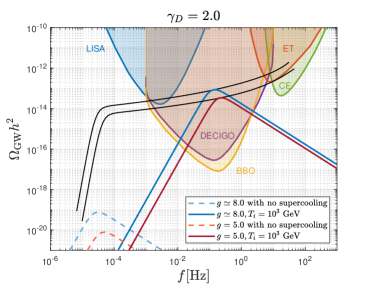
Figure 12: GW power spectra compared to the sensitivities of the prospected GW interferometers Schmitz:2020syl . The black solid curves seen around the centers of the plots draw the trajectories following the shift of the peak frequency generated by varying $T_{i}$ from $1.5\times 10^{-2}$ MeV to $1.0\times 10^{6}$ GeV. The dashed curves around the bottom of the figure correspond to the case where the supercooling effect in the dark sector (to supply the EW scale) is no longer left in the QCD phase transition epoch.

In Fig. 12 we show the GW spectra predicted from the supercooling phase transition in the topponium - Higgs coupled system around the QCD phase transition epoch. As seen from the figure, we have observed no significant dependence of $\gamma_{D}$ in the range of $0<\gamma_{D}\leq 2$. The produced GW spectra can be probed by the LISA, DECIGO, BBO, CE, and ET depending on the dark-sector energy-density scale characterized by $T_{i}$. The signals will be present in addition to those arising from the supercooling in the dark sector (scalegenesis) phase transition as discussed in the literature Iso:2017uuu ; Hambye:2018qjv ; Sagunski:2023ynd ; Dichtl:2023xqd ; Frandsen:2022klh ; Ellis:2022lft ; Bodeker:2021mcj ; vonHarling:2017yew . Just as a reference, also has been drawn the curves without the dark sector contribution (dashed curves around the bottom of the figure).

V Summary and discussions

In summary, we have made the first attempt to employ the nonperturbative analysis of the QCD-induced EW phase transition scenario, based on the LSD equations and the CJT formalism in the gauge-Higgs-Yukawa system. We have observed that the chiral broken QCD vacuum emerges with the nonperturbative top quark condensate, which can essentially be generated by the QCD sector: the EW phase transition at the QCD scale can be mainly triggered by QCD, even taking into account the strong top Yukawa interaction. Thus all the six quarks get masses small enough compared to the typical QCD critical temperature of the order of 100 MeV, where even the top quark can merely be in the same order (Fig.(7)). This is due to the big suppression of the top-Yukawa contributions to the ladder kernel caused by an accidental U(1) axial symmetry present in the top-Higgs Yukawa sector (Fig.3).

We then have discussed the impact on the top quark condensation in the QCD-EW phase transition by employing a quark-meson model-like description as the low-energy effective theory. There the SM Higgs couples with the mean field of the top quark condensate and topponium-like scalar bound state. The nonperturbative scale anomaly induced from the dynamical top quark condensation based on the LSD analysis as well as the associated nonperturbative results have been encoded in the quark meson model, which highly constrains the model parameter space. we have observed the EW phase transition of the first order type along the topponium - Higgs hybrid direction in the field space (Figs. 10) and (11). We have discussed the associated GW productions and found that in addition to the conventional GW signals sourced from an expected BSM at around or over the TeV scale, the dynamical topponium-Higgs system can yield another power spectrum sensitive to the BBO and LISA, and DECIGO, etc (Fig. 12).

Thus the presence of the nonperturbative top quark condensation in the supercooled EW phase transition would leave cosmologically probable footprints in the thermal history of the universe as the prospected GW spectra. This finding has presently been bench-marked based on the LSD method coupled with the quark meson-like and mean-field approach, which will pave a way to pursuing the QCD-origin cosmology coupled with possible BSM embedded in the classically scale-invariant scenario. In closing, we give several comments related to improvements from the present analysis, which is in more detail to be addressed in another publication.

Figure 13: A Feynman diagram generating the kinetic term mixing between $\sigma_{t}$ and $\sigma_{h}$ beyond the ladder approximation. The round blob attached on the $\sigma_{h}$ - $t$ - $t$ vertex, includes non-ladder corrections, in contrast to the ladder Fig. 9, generating the $\langle\sigma_{t}\rangle$ - $\langle\sigma_{h}\rangle$ mixing, constructed only from the ladder graphs.

• In the present work, the thermal corrections to the top-Higgs system have been taken into account in the quark-meson model, where a couple of the results from the LSD analysis have been used as inputs to fix the model parameters. The straightforward incorporation of the thermal corrections in the LSD analysis is possible and provides the temperature dependence of the top and bottom quarks along with the Higgs VEV $\sigma_{h}$. Thus we could have discussed both QCD and EW phase transitions solely in the LSD framework, not invoking the mean field (or bosonization of $\bar{t}t$) $\sigma_{t}$ or passing the quark meson model. However, the cosmological phase transition issue currently seems to be challenging to argue without the bounce scalar action or the false vacuum decay via the scalar field theory, namely, without $\sigma_{t}$. This issue will be addressed in future work.

• The LSD analysis can be improved by coupling to the functional renormalization group method, as has been discussed in Gao:2020qsj . It would be noteworthy to examine how non-ladder diagram corrections, incorporated into by the functional renormalization group, can affect the criticality of the top quark condensation and the thermal QCD and EW phase transitions.

• The significant topponium effect on the EW phase transition arises from the mixing with the SM Higgs as depicted in Fig. 9. This is essentially generated via the condensate mixture; $\langle\sigma_{t}\rangle$ - $\langle\sigma_{h}\rangle$, at the ladder approximation level, which thus contributes to the mean field potential as in Eq.(25). The kinetic term mixing can also generically be generated in the full gauge-Higgs-Yukawa theory, however, which goes beyond the ladder approximation because it is necessary to include the Yukawa vertex corrections. See Fig. 13. This beyond-the-ladder kinetic term mixing at finite temperature would modify the bounce action Eq.(36), which might give a nontrivial correction to the nucleation and percolation processes in the cosmological phase transition. Similar kinetic term corrections have been addressed in the literature Sagunski:2023ynd ; Aoki:2019mlt based on the Nambu-Jona-Lasinio type model for a dark QCD theory, in which, however, the kinetic mixing effect has been disregarded in the bounce equation. This issue is intriguing to be discussed in detail elsewhere.

References

- (1) G. Agazie, et al., The NANOGrav 15 yr Data Set: Evidence for a Gravitational-wave Background, Astrophys. J. Lett. 951 (1) (2023) L8. arXiv:2306.16213, doi:10.3847/2041-8213/acdac6.
- (2) G. Agazie, et al., The NANOGrav 15 yr Data Set: Constraints on Supermassive Black Hole Binaries from the Gravitational-wave Background, Astrophys. J. Lett. 952 (2) (2023) L37. arXiv:2306.16220, doi:10.3847/2041-8213/ace18b.
- (3) A. Afzal, et al., The NANOGrav 15 yr Data Set: Search for Signals from New Physics, Astrophys. J. Lett. 951 (1) (2023) L11. arXiv:2306.16219, doi:10.3847/2041-8213/acdc91.
- (4) J. Antoniadis, et al., The second data release from the European Pulsar Timing Array - I. The dataset and timing analysis, Astron. Astrophys. 678 (2023) A48. arXiv:2306.16224, doi:10.1051/0004-6361/202346841.
- (5) J. Antoniadis, et al., The second data release from the European Pulsar Timing Array - II. Customised pulsar noise models for spatially correlated gravitational waves, Astron. Astrophys. 678 (2023) A49. arXiv:2306.16225, doi:10.1051/0004-6361/202346842.
- (6) J. Antoniadis, et al., The second data release from the European Pulsar Timing Array - III. Search for gravitational wave signals, Astron. Astrophys. 678 (2023) A50. arXiv:2306.16214, doi:10.1051/0004-6361/202346844.
- (7) D. J. Reardon, et al., Search for an Isotropic Gravitational-wave Background with the Parkes Pulsar Timing Array, Astrophys. J. Lett. 951 (1) (2023) L6. arXiv:2306.16215, doi:10.3847/2041-8213/acdd02.
- (8) D. J. Reardon, et al., The Gravitational-wave Background Null Hypothesis: Characterizing Noise in Millisecond Pulsar Arrival Times with the Parkes Pulsar Timing Array, Astrophys. J. Lett. 951 (1) (2023) L7. arXiv:2306.16229, doi:10.3847/2041-8213/acdd03.
- (9) H. Xu, et al., Searching for the Nano-Hertz Stochastic Gravitational Wave Background with the Chinese Pulsar Timing Array Data Release I, Res. Astron. Astrophys. 23 (7) (2023) 075024. arXiv:2306.16216, doi:10.1088/1674-4527/acdfa5.
- (10) P. Amaro-Seoane, et al., Laser Interferometer Space Antenna (2 2017). arXiv:1702.00786.
- (11) C. Caprini, et al., Detecting gravitational waves from cosmological phase transitions with LISA: an update, JCAP 03 (2020) 024. arXiv:1910.13125, doi:10.1088/1475-7516/2020/03/024.
- (12) V. Corbin, N. J. Cornish, Detecting the cosmic gravitational wave background with the big bang observer, Class. Quant. Grav. 23 (2006) 2435–2446. arXiv:gr-qc/0512039, doi:10.1088/0264-9381/23/7/014.
- (13) G. M. Harry, P. Fritschel, D. A. Shaddock, W. Folkner, E. S. Phinney, Laser interferometry for the big bang observer, Class. Quant. Grav. 23 (2006) 4887–4894, [Erratum: Class.Quant.Grav. 23, 7361 (2006)]. doi:10.1088/0264-9381/23/15/008.
- (14) S. Kawamura, et al., The Japanese space gravitational wave antenna DECIGO, Class. Quant. Grav. 23 (2006) S125–S132. doi:10.1088/0264-9381/23/8/S17.
- (15) K. Yagi, N. Seto, Detector configuration of DECIGO/BBO and identification of cosmological neutron-star binaries, Phys. Rev. D 83 (2011) 044011, [Erratum: Phys.Rev.D 95, 109901 (2017)]. arXiv:1101.3940, doi:10.1103/PhysRevD.83.044011.
- (16) Y. Aoki, S. Borsanyi, S. Durr, Z. Fodor, S. D. Katz, S. Krieg, K. K. Szabo, The QCD transition temperature: results with physical masses in the continuum limit II., JHEP 06 (2009) 088. arXiv:0903.4155, doi:10.1088/1126-6708/2009/06/088.
- (17) S. Borsanyi, G. Endrodi, Z. Fodor, C. Hoelbling, S. Katz, S. Krieg, C. Ratti, K. K. Szabo, Transition temperature and the equation of state from lattice QCD, Wuppertal-Budapest results, J. Phys. Conf. Ser. 316 (2011) 012020. arXiv:1109.5032, doi:10.1088/1742-6596/316/1/012020.
- (18) H.-T. Ding, F. Karsch, S. Mukherjee, Thermodynamics of strong-interaction matter from Lattice QCD, Int. J. Mod. Phys. E 24 (10) (2015) 1530007. arXiv:1504.05274, doi:10.1142/S0218301315300076.
- (19) A. Bazavov, et al., Chiral crossover in QCD at zero and non-zero chemical potentials, Phys. Lett. B 795 (2019) 15–21. arXiv:1812.08235, doi:10.1016/j.physletb.2019.05.013.
- (20) H.-T. Ding, New developments in lattice QCD on equilibrium physics and phase diagram, Nucl. Phys. A 1005 (2021) 121940. arXiv:2002.11957, doi:10.1016/j.nuclphysa.2020.121940.
- (21) A. Bazavov, N. Brambilla, H. T. Ding, P. Petreczky, H. P. Schadler, A. Vairo, J. H. Weber, Polyakov loop in 2+1 flavor QCD from low to high temperatures, Phys. Rev. D 93 (11) (2016) 114502. arXiv:1603.06637, doi:10.1103/PhysRevD.93.114502.
- (22) H.-T. Ding, Lattice QCD at nonzero temperature and density, PoS LATTICE2016 (2017) 022. arXiv:1702.00151, doi:10.22323/1.256.0022.
- (23) S. Iso, P. D. Serpico, K. Shimada, QCD-Electroweak First-Order Phase Transition in a Supercooled Universe, Phys. Rev. Lett. 119 (14) (2017) 141301. arXiv:1704.04955, doi:10.1103/PhysRevLett.119.141301.
- (24) T. Hambye, A. Strumia, D. Teresi, Super-cool Dark Matter, JHEP 08 (2018) 188. arXiv:1805.01473, doi:10.1007/JHEP08(2018)188.
- (25) B. von Harling, G. Servant, QCD-induced Electroweak Phase Transition, JHEP 01 (2018) 159. arXiv:1711.11554, doi:10.1007/JHEP01(2018)159.
- (26) M. Dichtl, J. Nava, S. Pascoli, F. Sala, Baryogenesis and leptogenesis from supercooled confinement, JHEP 02 (2024) 059. arXiv:2312.09282, doi:10.1007/JHEP02(2024)059.
- (27) J. Ellis, M. Lewicki, M. Merchand, J. M. No, M. Zych, The scalar singlet extension of the Standard Model: gravitational waves versus baryogenesis, JHEP 01 (2023) 093. arXiv:2210.16305, doi:10.1007/JHEP01(2023)093.
- (28) X.-R. Wang, J.-Y. Li, S. Enomoto, H. Ishida, S. Matsuzaki, QCD preheating: New frontier of baryogenesis, Phys. Rev. D 108 (2) (2023) 023512. arXiv:2206.00519, doi:10.1103/PhysRevD.108.023512.
- (29) L. Sagunski, P. Schicho, D. Schmitt, Supercool exit: Gravitational waves from QCD-triggered conformal symmetry breaking, Phys. Rev. D 107 (12) (2023) 123512. arXiv:2303.02450, doi:10.1103/PhysRevD.107.123512.
- (30) M. T. Frandsen, M. Heikinheimo, M. E. Thing, K. Tuominen, M. Rosenlyst, Vector dark matter in supercooled Higgs portal models, Phys. Rev. D 108 (1) (2023) 015033. arXiv:2301.00041, doi:10.1103/PhysRevD.108.015033.
- (31) D. Bödeker, Remarks on the QCD-electroweak phase transition in a supercooled universe, Phys. Rev. D 104 (11) (2021) L111501. arXiv:2108.11966, doi:10.1103/PhysRevD.104.L111501.
- (32) J. M. Cornwall, R. Jackiw, E. Tomboulis, Effective Action for Composite Operators, Phys. Rev. D 10 (1974) 2428–2445. doi:10.1103/PhysRevD.10.2428.
- (33) R. L. Workman, et al., Review of Particle Physics, PTEP 2022 (2022) 083C01. doi:10.1093/ptep/ptac097.
- (34) K.-i. Kondo, A. Shibata, M. Tanabashi, K. Yamawaki, Phase structure of the gauged Yukawa model, Prog. Theor. Phys. 91 (1994) 541–572, [Erratum: Prog.Theor.Phys. 93, 489 (1995)]. arXiv:hep-ph/9312322, doi:10.1143/ptp/91.3.541.
- (35) V. A. Miransky, Dynamical symmetry breaking in quantum field theories, 1994.
- (36) H. Pagels, S. Stokar, The Pion Decay Constant, Electromagnetic Form-Factor and Quark Electromagnetic Selfenergy in QCD, Phys. Rev. D 20 (1979) 2947. doi:10.1103/PhysRevD.20.2947.
- (37) A. Deur, S. J. Brodsky, C. D. Roberts, QCD running couplings and effective charges, Prog. Part. Nucl. Phys. 134 (2024) 104081. arXiv:2303.00723, doi:10.1016/j.ppnp.2023.104081.
- (38) Y.-L. Li, Y.-L. Ma, M. Rho, Chiral-scale effective theory including a dilatonic meson, Phys. Rev. D 95 (11) (2017) 114011. arXiv:1609.07014, doi:10.1103/PhysRevD.95.114011.
- (39) O. Catà, C. Müller, Chiral effective theories with a light scalar at one loop, Nucl. Phys. B 952 (2020) 114938. arXiv:1906.01879, doi:10.1016/j.nuclphysb.2020.114938.
- (40) R. Zwicky, QCD with an infrared fixed point: The pion sector, Phys. Rev. D 109 (3) (2024) 034009. arXiv:2306.06752, doi:10.1103/PhysRevD.109.034009.
- (41) R. Zwicky, QCD with an Infrared Fixed Point and a Dilaton (12 2023). arXiv:2312.13761.
- (42) R. J. Crewther, Genuine Dilatons in Gauge Theories, Universe 6 (7) (2020) 96. arXiv:2003.11259, doi:10.3390/universe6070096.
- (43) R. J. Crewther, L. C. Tunstall, rule for kaon decays derived from QCD infrared fixed point, Phys. Rev. D 91 (3) (2015) 034016. arXiv:1312.3319, doi:10.1103/PhysRevD.91.034016.
- (44) S. R. Coleman, E. J. Weinberg, Radiative Corrections as the Origin of Spontaneous Symmetry Breaking, Phys. Rev. D 7 (1973) 1888–1910. doi:10.1103/PhysRevD.7.1888.
- (45) A. D. Linde, Decay of the False Vacuum at Finite Temperature, Nucl. Phys. B 216 (1983) 421, [Erratum: Nucl.Phys.B 223, 544 (1983)]. doi:10.1016/0550-3213(83)90072-X.
- (46) A. J. Helmboldt, J. Kubo, S. van der Woude, Observational prospects for gravitational waves from hidden or dark chiral phase transitions, Phys. Rev. D 100 (5) (2019) 055025. arXiv:1904.07891, doi:10.1103/PhysRevD.100.055025.
- (47) C. L. Wainwright, CosmoTransitions: Computing Cosmological Phase Transition Temperatures and Bubble Profiles with Multiple Fields, Comput. Phys. Commun. 183 (2012) 2006–2013. arXiv:1109.4189, doi:10.1016/j.cpc.2012.04.004.
- (48) A. H. Guth, S. H. H. Tye, Phase Transitions and Magnetic Monopole Production in the Very Early Universe, Phys. Rev. Lett. 44 (1980) 631, [Erratum: Phys.Rev.Lett. 44, 963 (1980)]. doi:10.1103/PhysRevLett.44.631.
- (49) A. H. Guth, E. J. Weinberg, Cosmological Consequences of a First Order Phase Transition in the SU(5) Grand Unified Model, Phys. Rev. D 23 (1981) 876. doi:10.1103/PhysRevD.23.876.
- (50) J. Ellis, M. Lewicki, J. M. No, On the Maximal Strength of a First-Order Electroweak Phase Transition and its Gravitational Wave Signal, JCAP 04 (2019) 003. arXiv:1809.08242, doi:10.1088/1475-7516/2019/04/003.
- (51) V. Brdar, A. J. Helmboldt, J. Kubo, Gravitational Waves from First-Order Phase Transitions: LIGO as a Window to Unexplored Seesaw Scales, JCAP 02 (2019) 021. arXiv:1810.12306, doi:10.1088/1475-7516/2019/02/021.
- (52) H.-X. Zhang, S. Matsuzaki, H. Ishida, Gravitational wave footprints from Higgs-portal scalegenesis with multiple dark chiral scalars*, Chin. Phys. C 48 (4) (2024) 045106. arXiv:2401.00771, doi:10.1088/1674-1137/ad2b4f.
- (53) K. Schmitz, New Sensitivity Curves for Gravitational-Wave Signals from Cosmological Phase Transitions, JHEP 01 (2021) 097. arXiv:2002.04615, doi:10.1007/JHEP01(2021)097.
- (54) F. Gao, J. M. Pawlowski, QCD phase structure from functional methods, Phys. Rev. D 102 (3) (2020) 034027. arXiv:2002.07500, doi:10.1103/PhysRevD.102.034027.
- (55) M. Aoki, J. Kubo, Gravitational waves from chiral phase transition in a conformally extended standard model, JCAP 04 (2020) 001. arXiv:1910.05025, doi:10.1088/1475-7516/2020/04/001.