A nonlinear criterion for characterizing high-dimensional multipartite entanglement
Abstract
Understanding entanglement of potentially high-dimensional multipartite quantum systems is crucial across different disciplines in quantum sciences. We take inspiration from covariance matrix based techniques to derive a nonlinear criterion that can be used to lower bound the dimensionality vector of mixed quantum states, revealing both the level of multipartiteness and the dimensionality of the entanglement in the quantum states. The technique is based on a system of inequalities that has to be satisfied by all quantum states with a given entanglement dimensionality vector, which can be checked via linear programming. We test our condition on paradigmatic classes of high-dimensional multipartite entangled states like imperfect Greenberger-Horne-Zeilinger (GHZ) states and find that, in comparison with other available criteria our method provides a significant advantage, which is enhanced especially in the case that the dimensions of the individual particles are different from each other.
Quantification of entanglement is a topic of wide interest crossing various areas of physics, because of its foundational interest, its connection to thermodynamics and also because of its deep connections with several quantum information problems [1, 2, 3, 4, 5, 6]. The task is highly non-trivial and has become subject of intense investigation starting from the case of two particles of relatively small dimension, but reaches a daunting complexity when either or both the number of particles or the particles’ dimensions increase.
In fact, multipartite entanglement is very complex to even characterize qualitatively since different inequivalent notions can be given and its classification is known to be itself a very complex subject [7]. Beyond its classification, important questions are how to witness the various forms of multipartite entanglement and how to properly quantify it. Due to the complex structure of multipartite entangled states it is often not possible to provide a satisfactory quantification with only a single number, but it is better to consider entanglement monotones across some set of bipartitions. Concrete entanglement monotones considered are convex-roof extended entropies of marginal states, which are defined first for pure states as follows.
Taking first a given bipartition we consider the entropy of the single-party marginal:
| (1) |
where is a given entropy, like e.g., the linear entropy , the von Neumann entropy , or the zero entropy . For a single bipartition, these measures are then extended to mixed states via convex-roof, i.e., by taking the minimum over all possible decompositions into pure states. It is here that the complexity of all entanglement quantification tasks originates: (almost) all states feature an infinite number of possible decompositions, or equivalently, an infinite set of possible preparations that lead to the experimental situation described by the density matrix. So the convex roof basically corresponds to the worst-case scenario among all the possible pure-state decompositions, i.e., which preparation needs the least amount of entanglement. Clearly, this makes it quite complex in practical scenarios to calculate, since considering all possible (infinitely many) pure-state decompositions of a density matrix is in general a very challenging task, leading to the NP-hardness of entanglement certification [8].
In the multipartite scenario, all the above-mentioned difficulties to quantify entanglement are exacerbated, as each decomposition element might now feature different factorisations. Hence, in order to characterize and properly quantify the genuinely multipartite nature of the entanglement in the state it is important not only to consider the full set of bipartitions, but also to take the worst-case scenario amongst all possible mixtures of states entangled in different ways in the different bipartitions. This translates into considering the vector of entropies of the reductions for all possible bipartitions, which can be enumerated with an index going from to for a -particle system, and moreover order such a vector, for example non-increasingly. This way, one defines measures like
| (2) |
where are the components of the vector of entropies of the marginal states for all partitions and the infimum is taken over all pure state decompositions . Among all possible entanglement entropy vectors, only the von Neumann and the 0-entropy cases feature a nontrivial asymptotic structure that can be constrained by linear inequalities [9, 10, 11].
In this work, we will focus on the 0-entropy case, which is nothing but the logarithm of the rank of the density matrix, which, being discrete, is also a special case that allows for a better classification of the state as a resource as opposite to continuous measures [12, 13, 14]. This extends to multipartite states the concept of Schmidt number (or entanglement dimensionality) [15, 16] and, for example, is a necessary resource to achieve an exponential speedup in a pure-state quantum circuit [12, 17]. Concretely, for pure states, one defines the Schmidt-rank vector as the vector of Schmidt ranks with respect to all possible bipartitions
| (3) |
and then orders its elements non-increasingly. As we mentioned, the ordering becomes crucial for extending this notion to the multipartite case and for clarity we denote the ordered vectors by .
To be more clear, let us first recall the definition of a Genuinely Multipartite Entangled state, which is a state that is not biseparable. A biseparable state is defined as a mixture of states that are separable across (at least) one partition, which can be different for the different decomposition elements. Such a state has an entanglement-dimensionality vector such that its last (smallest) component is one, i.e., . More in general, then, one defines the entanglement-dimensionality vector element-wise via the convex roof construction, i.e.,
| (4) |
with again the crucial requirement that the pure-state Schmidt-rank vector is ordered non-increasingly. In other words, a density matrix has whenever it has a pure-state decomposition such that the -th largest Schmidt rank among all possible bipartitions is always smaller than or equal to . Thus, overall a density matrix with entanglement-dimensionality vector given by can be decomposed as
| (5) |
where are probabilities and are states with a given (unordered) Schmidt number vector that is such that its components, when ordered non-increasingly, satisfy .
This definition creates a structure of states with different entanglement dimensionality vectors which is far more complex than that arising in the bipartite case, especially because it is not simply formed by nested convex sets contained into each other. In particular, it is not possible to order all the different entanglement dimensionality vectors, even though the states having a particular still form a convex set. See fig. 1 for a pictorial representation.
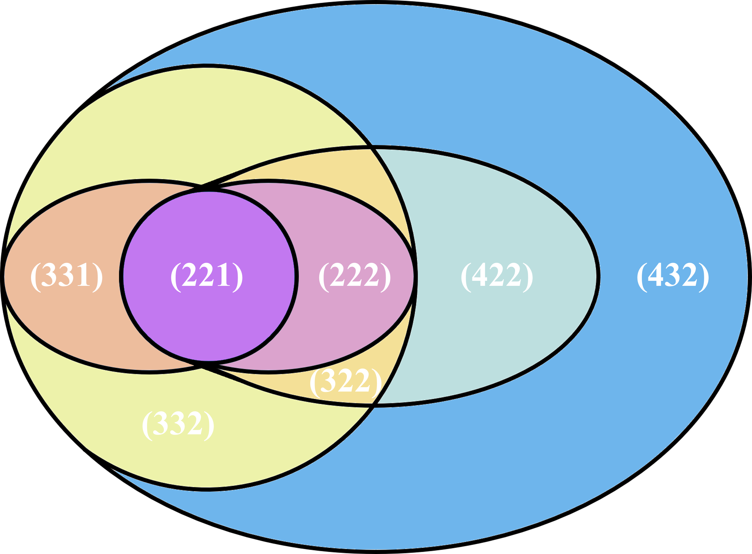
Furthermore, Schmidt numbers across different bipartitions satisfy highly nontrivial relations amongst each other, also depending on the dimensions and number of particles [11]. These are analogous to the so-called monogamy relations arising between bipartite and multipartite entanglement monotones in a multipartite state [18]. Because of this, usual methods to witness the Schmidt number become much more complex when extended to the multipartite case, and thus there is a lack of efficient methods to characterize the full entanglement dimensionality vector in general [19, 13, 14].
Thus, it would be extremely interesting to provide new approaches to characterize the entanglement-dimensionality vector. This is also further motivated from the fact that high-dimensional multipartite entanglement is known to be a resource for a number of tasks, like high-dimensional quantum teleportation [20], stronger violation of multipartite Bell inequalities [21, 22, 23, 24, 25], generation of increased randomness [26] and increased Quantum Key-Distribution (QKD) rates [27, 28, 29, 30, 31]. In fact, high-dimensional multipartite entangled states have been the target of numerous recent experiments, particularly with photonic systems [32, 33, 34, 35, 20, 36, 37, 38, 39, 26, 40, 41, 42, 43, 44, 45, 46, 47, 48, 49, 50, 51, 52, 29, 53, 54, 55, 56, 57, 58, 59].
Typical witnesses of the entanglement-dimensionality vector are given in terms of fidelities with respect to target states [32]. Concretely, given a certain (non-increasingly ordered) entanglement dimensionality vector and a certain target state one defines the maximum fidelity with a generic density matrix with :
| (6) |
where is a generic pure state with ordered Schmidt-rank vector given by and the equality follows from convexity of the fidelity. Then, whenever one finds that
| (7) |
one can conclude that is outside of the set of states with entanglement dimensionality vector given by .
Note once more however, that one cannot generally conclude that has a particular entanglement-dimensionality vector which is “greater” than , because such an ordering is lost in the multipartite case. Furthermore, even though the fidelity is a convex function of the state and therefore to calculate its maximum in Eq. 6 one can restrict to pure states, one needs to know the Schmidt eigenvalues of the target state across all bipartitions and, even after that, perform in general a quite demanding optimization. See Supplemental Material for more details [60]. This is because one needs to consider pure states with many different Schmidt-number vectors. A great simplification to this task can come from choosing a target state which is highly symmetric, a typical example being the Greenberger-Horne-Zeilinger (GHZ) state:
| (8) |
The simplification comes from the fact that the state is invariant under permutation of the parties and the one-body marginals are all maximally mixed.
With such a target state the bound coincides for all entanglement-dimensionality vectors that have a given . In general this is one of the few examples for which the bound in Eq. 6 is known and can thus be applied to practical entanglement detection. Beyond fidelities, nonlinear witnesses of the entanglement dimensionality vector have been derived in [13, 61], which we summarize in the Supplemental Material [60] and later compare to our criterion. These are essentially all criteria that exist to witness the entanglement-dimensionality vector. Because of this, it is useful to find alternative criteria, especially some that would be readily applicable even without further optimization.
Our approach is based on an alternative method that has been extended recently to witness the Schmidt number across bipartitions, called Covariance Matrix Criterion (CMC) [62, 63, 64, 65, 66], which is written in terms of the covariance matrix of an orthonormal operator basis for each party. Here, working explicitly in a multipartite setting, we consider single-particle operators that satisfy . Given a bipartition we can construct basis for a party by simply taking tensor products of single-particle operators among all the particles in : . To be more clear and compact, we used a single capitalized index for such a basis.
First, let us fix a bipartition and consider the cross-covariances
| (9) |
on a quantum state . Using the results of [62] (generalizing those of [64, 65, 66]) we know that one important corollary of the CMC is given by the following expression, which is invariant under change of bases for the parties :
| (10) |
where is the trace norm of a matrix and we named the left-hand side as to shorten the notation in the following. Eq. 10 must hold for all states that have Schmidt number at most equal to across partition .
Now, let us try to extend such a relation to detect the entire entanglement dimensionality vector. For that, we need to consider all partitions at the same time, and correspondingly all matrices labelled by the different bipartitions and obtain the following result:
Observation 1.
Let us consider the functions as defined in Eq. 10. Every density matrix that has an entanglement dimensionality vector given by must satisfy the following system of equations:
| (11) | ||||
where is a vector of real numbers such that
| (12) |
which means that
| (13) |
where are the elements of ordered non-increasingly. This system of equations can be solved with a linear program in the variables . If no solution to this problem can be found, then the state cannot have entanglement dimensionality vector given by .
The technical details of the proof of this statement can be found in the Supplemental Material [60]. Note that a similar idea can be applied to other corollaries of the CMC potentially, whenever they are found, which is a task that we leave for further investigation. Here we just consider Eq. 10 as a prototypical example which is relevant for concrete situations. Note also that simpler conditions can be obtained from this system of equations, e.g., by summing up all equations and obtaining:
| (14) |
An even simpler criterion can be derived from Eq. 10 by further bounding its left-hand side. Consider orthonormal bases of the single particle operator space for each particle and let be the smallest among the single-particle dimensions. The following inequality
| (15) |
must be satisfied by all states that are such that the last element of their entanglement dimensionality vector is given by . Thus, a violation of this inequality implies that has the minimal entanglement dimensionality which is larger than . This condition simply follows from the fact that the left-hand side of Eq. 10, i.e., is larger than that of Eq. 15 for every . Thus, we can take the minimum among all and we obtain that Eq. 15 is valid for pure states. At the same time, the left-hand side is linear under mixing the quantum state and thus it is immediately extended to all density matrices. In this derivation, we can also observe the important difference with respect to Eq. 11: Taking the expression is by itself neither linear nor concave under mixing the quantum state. Thus, even though the analogous condition as in Eq. 15 holds for pure states, it cannot be readily extended to mixed states of the form (5). For that, it was needed to consider the whole set with the corresponding bounds changing from the set of to a set of real number that only has to satisfy a weaker constraint .
As a result, we get two independent conditions, Eqs. 11 and 15 that provide complementary information about the entanglement-dimensionality vector, as we will clarify afterwards with some examples. In particular, the condition in Eq. 15 it is nothing but the fidelity bound with respect to a target state of the form
| (16) |
which is such that its single-particle marginals are all maximally mixed (such a state is called -uniform in the literature about multipartite entanglement classification [67, 68, 69]), and in that sense is analogous to the GHZ state. A detailed proof of Eq. 15 and its relation with fidelities to -uniform states can be found in the Supplemental Material [60].
Let us now investigate the practical applicability of our results, also in comparison with other methods. First of all, it is clear that the combination of the two inequalities (11,15) provides a witness which is stronger than the fidelity witness with respect to an optimal -uniform state that depends on . Moreover, although it is hard to make fully general statements due to the variety and complexity of all the potential cases, we can observe that our method outperforms also the other known entanglement-dimensionality witnesses, at least in several important cases. First of all, we can consider the most common example of high-dimensional multipartite entangled states, which are GHZ states mixed with white noise. The noiseless case is actually a very important target state [35, 70, 71, 72, 73, 74, 75] for several tasks in which distribution of entanglement is required among many parties, for example error-correction [67, 68, 69] and quantum communication [32], and the white noise provides a general worst-case scenario for practical imperfections. In fact, known witnesses for genuine multipartite entanglement were tested on these states [76, 77, 19].
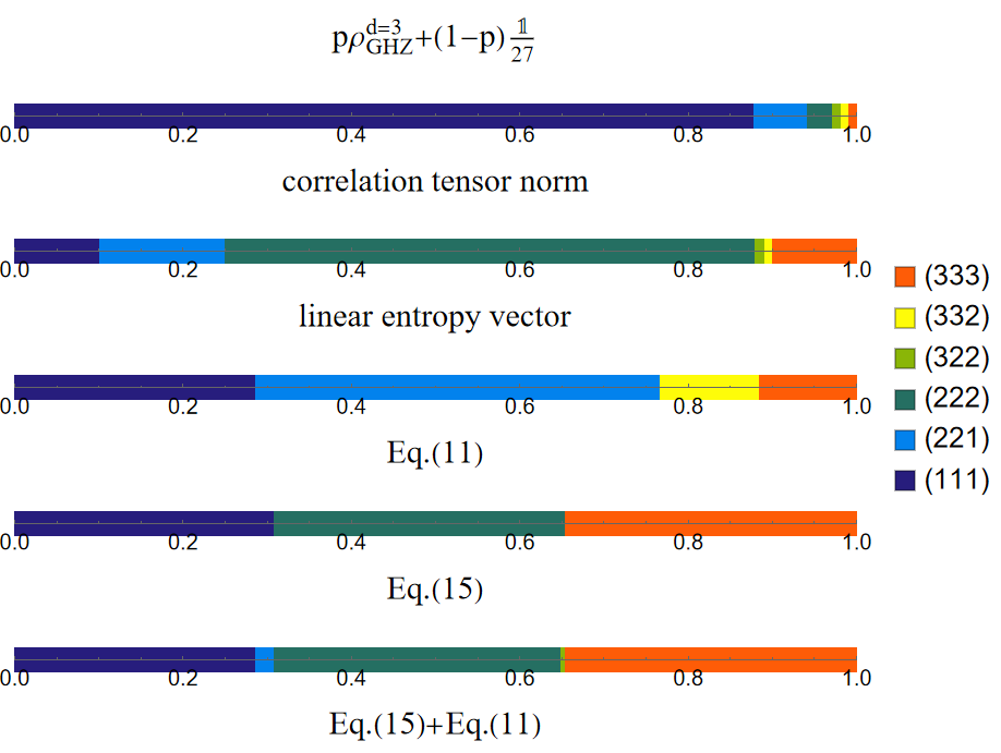
In fig. 2 we make an explicit comparison among all known methods and we can see that there is a noise region in which Eq. 11 actually improves the detection of the whole entanglement-dimensionality vector as compared to the fidelity witness alone. All other methods are also clearly weaker in this case.
Besides this important paradigmatic case, we tested our method on other example states and randomly sampled states and we can summarize our findings as follows. In short, we find that our criterion is significantly advantageous when the dimension of one subsystem is higher than that of all other subsystems. Let us elucidate that with a concrete example. Consider the Hilbert space and the following pure state, that has a Schmidt number vector :
| (17) |
where is a unit vector of complex coefficients. The case with all was considered in [13] as a simple paradigmatic example to show the partial ordering structure of the Schmidt number vector . In our simulations we then mix such randomly sampled pure states with white noise and consider the state
| (18) |
We then try to detect the state mixed with white noise using Eq. 11 and the fidelity with respect to for comparison. All other criteria mentioned earlier are worse than either our method or the fidelity with respect to . To certify , one must exclude and simultaneously, while these two subsets are not comparable, i.e., they are addressed by two bounds individually. We make this comparison between the two criteria using completely random coefficients across a total of 10000 samples. We use t-Distributed Stochastic Neighbor Embedding (t-SNE) [78] as a dimension reduction technique to show the sample data. This is a method that ensures that states with coefficient vectors that are close to each other, remain close also in the lower-dimensional projected figure. The results are shown in fig. 3.
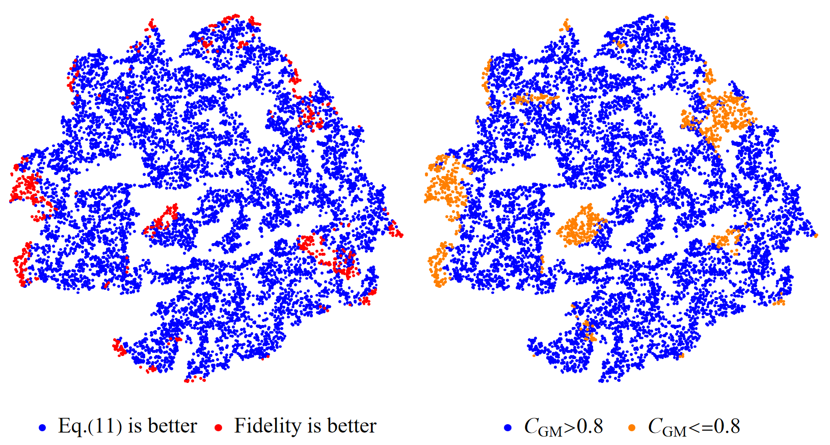
As shown in the plot, our method outperforms the fidelity witness in most of the cases (about ). It is also worth noting that the points that are detected by our method mostly coincide with states that have a relatively high value of the so-called genuine multipartite concurrence, which is defined as the lowest element of the entropy vector in Eq. 2 where the entropy of choice is the linear entropy [79, 80, 81]:
| (19) |
However, notice that is not high enough to witness a better than either our criterion (11) or the fidelity with respect to .
In conclusion, we have presented a new approach to find witnesses for the entanglement dimensionality vector in multipartite systems, which is based on extending corollaries of the bipartite Covariance Matrix Criterion to the multipartite case. We have applied this idea explicitly to a known corollary of the CMC, which leads to a criterion that is strictly stronger than fidelity witnesses with respect to -uniform states such as the GHZ states, which represent in practice the most widely used witnesses. Moreover, we have shown that this criterion also improves over known methods on a wide class of states, which include important paradigmatic examples useful for applications. Further developments of our approach can be obtained by finding new corollaries to the CMC, or in general nonlinear witnesses of the Schmidt number in the bipartite case, which thus represents a promising direction for further research in this topic.
Acknowledgments.—This work is supported by the National Natural Science Foundation of China (Grants No. 12125402), the Innovation Program for Quantum Science and Technology (No. 2021ZD0301500) and the China Postdoctoral Science Foundation (No. 2023M740119). GV acknowledges financial support from the Austrian Science Fund (FWF) through the grants P 35810-N and P 36633-N (Stand-Alone). M.H. acknowledges support from the Horizon-Europe research and innovation programme under grant agreement No 101070168 (HyperSpace).
References
- Horodecki et al. [2009] R. Horodecki, P. Horodecki, M. Horodecki, and K. Horodecki, Quantum entanglement, Rev. Mod. Phys. 81, 865 (2009).
- Amico et al. [2008] L. Amico, R. Fazio, A. Osterloh, and V. Vedral, Entanglement in many-body systems, Rev. Mod. Phys. 80, 517 (2008).
- Gühne and Tóth [2009] O. Gühne and G. Tóth, Entanglement detection, Phys. Rep. 474, 1 (2009).
- Laflorencie [2016] N. Laflorencie, Quantum entanglement in condensed matter systems, Phys. Rep. 646, 1 (2016).
- Friis et al. [2019] N. Friis, G. Vitagliano, M. Malik, and M. Huber, Entanglement certification from theory to experiment, Nat. Rev. Phys. 1, 72 (2019).
- Raussendorf and Briegel [2001] R. Raussendorf and H. J. Briegel, A one-way quantum computer, Phys. Rev. Lett. 86, 5188 (2001).
- Eltschka and Siewert [2014] C. Eltschka and J. Siewert, Quantifying entanglement resources, J. Phys. A: Math. Theor. 47, 424005 (2014).
- Gurvits [2003] L. Gurvits, Classical deterministic complexity of Edmonds’ Problem and quantum entanglement, in Proceedings of the Thirty-Fifth Annual ACM Symposium on Theory of Computing (Association for Computing Machinery), STOC ’03, 10–19 (2003).
- Lieb and Ruskai [1973a] E. H. Lieb and M. B. Ruskai, A fundamental property of quantum-mechanical entropy, Phys. Rev. Lett. 30, 434 (1973a).
- Lieb and Ruskai [1973b] E. H. Lieb and M. B. Ruskai, Proof of the strong subadditivity of quantum‐mechanical entropy, J. Math. Phys. 14, 1938 (1973b).
- Cadney et al. [2014] J. Cadney, M. Huber, N. Linden, and A. Winter, Inequalities for the ranks of multipartite quantum states, Linear Algebra Appl. 452, 153 (2014).
- Van den Nest [2013] M. Van den Nest, Universal quantum computation with little entanglement, Phys. Rev. Lett. 110, 060504 (2013).
- Huber and de Vicente [2013] M. Huber and J. I. de Vicente, Structure of multidimensional entanglement in multipartite systems, Phys. Rev. Lett. 110, 030501 (2013).
- Huber et al. [2013] M. Huber, M. Perarnau-Llobet, and J. I. de Vicente, Entropy vector formalism and the structure of multidimensional entanglement in multipartite systems, Phys. Rev. A 88, 042328 (2013).
- Terhal and Horodecki [2000] B. M. Terhal and P. Horodecki, Schmidt number for density matrices, Phys. Rev. A 61, 040301 (2000).
- Sanpera et al. [2001] A. Sanpera, D. Bruß, and M. Lewenstein, Schmidt-number witnesses and bound entanglement, Phys. Rev. A 63, 050301 (2001).
- Vidal [2003] G. Vidal, Efficient classical simulation of slightly entangled quantum computations, Phys. Rev. Lett. 91, 147902 (2003).
- Osborne and Verstraete [2006] T. J. Osborne and F. Verstraete, General monogamy inequality for bipartite qubit entanglement, Phys. Rev. Lett. 96, 220503 (2006).
- Huber et al. [2010] M. Huber, F. Mintert, A. Gabriel, and B. C. Hiesmayr, Detection of high-dimensional genuine multipartite entanglement of mixed states, Phys. Rev. Lett. 104, 210501 (2010).
- Luo et al. [2019] Y.-H. Luo, H.-S. Zhong, M. Erhard, X.-L. Wang, L.-C. Peng, M. Krenn, X. Jiang, L. Li, N.-L. Liu, C.-Y. Lu, A. Zeilinger, and J.-W. Pan, Quantum teleportation in high dimensions, Phys. Rev. Lett. 123, 070505 (2019).
- Collins et al. [2002] D. Collins, N. Gisin, N. Linden, S. Massar, and S. Popescu, Bell inequalities for arbitrarily high-dimensional systems, Phys. Rev. Lett. 88, 040404 (2002).
- Ryu et al. [2013] J. Ryu, C. Lee, M. Żukowski, and J. Lee, Greenberger-horne-zeilinger theorem for qudits, Phys. Rev. A 88, 042101 (2013).
- Ryu et al. [2014] J. Ryu, C. Lee, Z. Yin, R. Rahaman, D. G. Angelakis, J. Lee, and M. Żukowski, Multisetting greenberger-horne-zeilinger theorem, Phys. Rev. A 89, 024103 (2014).
- Lawrence [2014] J. Lawrence, Rotational covariance and greenberger-horne-zeilinger theorems for three or more particles of any dimension, Phys. Rev. A 89, 012105 (2014).
- Tang et al. [2017] W. Tang, S. Yu, and C. H. Oh, Multisetting greenberger-horne-zeilinger paradoxes, Phys. Rev. A 95, 012131 (2017).
- Wang et al. [2018a] J. Wang, S. Paesani, Y. Ding, R. Santagati, P. Skrzypczyk, A. Salavrakos, J. Tura, R. Augusiak, L. Mančinska, D. Bacco, D. Bonneau, J. W. Silverstone, Q. Gong, A. Acín, K. Rottwitt, L. K. Oxenløwe, J. L. O’Brien, A. Laing, and M. G. Thompson, Multidimensional quantum entanglement with large-scale integrated optics, Science 360, 285 (2018a).
- Cerf et al. [2002] N. J. Cerf, M. Bourennane, A. Karlsson, and N. Gisin, Security of quantum key distribution using -level systems, Phys. Rev. Lett. 88, 127902 (2002).
- Gröblacher et al. [2006] S. Gröblacher, T. Jennewein, A. Vaziri, G. Weihs, and A. Zeilinger, Experimental quantum cryptography with qutrits, New J. Phys. 8, 75 (2006).
- Ecker et al. [2019] S. Ecker, F. Bouchard, L. Bulla, F. Brandt, O. Kohout, F. Steinlechner, R. Fickler, M. Malik, Y. Guryanova, R. Ursin, and M. Huber, Overcoming noise in entanglement distribution, Phys. Rev. X 9, 041042 (2019).
- Ali-Khan et al. [2007] I. Ali-Khan, C. J. Broadbent, and J. C. Howell, Large-alphabet quantum key distribution using energy-time entangled bipartite states, Phys. Rev. Lett. 98, 060503 (2007).
- Vértesi et al. [2010] T. Vértesi, S. Pironio, and N. Brunner, Closing the detection loophole in bell experiments using qudits, Phys. Rev. Lett. 104, 060401 (2010).
- Malik et al. [2016] M. Malik, M. Erhard, M. Huber, M. Krenn, R. Fickler, and A. Zeilinger, Multi-photon entanglement in high dimensions, Nat. Photonics 10, 248–252 (2016).
- Li et al. [2020] L. Li, Z. Liu, X. Ren, S. Wang, V.-C. Su, M.-K. Chen, C. H. Chu, H. Y. Kuo, B. Liu, W. Zang, G. Guo, L. Zhang, Z. Wang, S. Zhu, and D. P. Tsai, Metalens-array–based high-dimensional and multiphoton quantum source, Science 368, 1487 (2020).
- Chi et al. [2022] Y. Chi, J. Huang, Z. Zhang, J. Mao, Z. Zhou, X. Chen, C. Zhai, J. Bao, T. Dai, H. Yuan, et al., A programmable qudit-based quantum processor, Nat. Commun. 13, 1166 (2022).
- Erhard et al. [2018] M. Erhard, M. Malik, M. Krenn, and A. Zeilinger, Experimental greenberger–horne–zeilinger entanglement beyond qubits, Nat. Photonics 12, 759 (2018).
- Guo et al. [2018] Y. Guo, X.-M. Hu, B.-H. Liu, Y.-F. Huang, C.-F. Li, and G.-C. Guo, Experimental witness of genuine high-dimensional entanglement, Phys. Rev. A 97, 062309 (2018).
- Krenn et al. [2014] M. Krenn, M. Huber, R. Fickler, R. Lapkiewicz, S. Ramelow, and A. Zeilinger, Generation and confirmation of a (100 × 100)-dimensional entangled quantum system, Proc. Natl. Acad. Sci. U.S.A. 111, 6243 (2014).
- Dada et al. [2011] A. C. Dada, J. Leach, G. S. Buller, M. J. Padgett, and E. Andersson, Experimental high-dimensional two-photon entanglement and violations of generalized bell inequalities, Nat. Phys. 7, 677 (2011).
- Schaeff et al. [2015] C. Schaeff, R. Polster, M. Huber, S. Ramelow, and A. Zeilinger, Experimental access to higher-dimensional entangled quantum systems using integrated optics, Optica 2, 523 (2015).
- Martin et al. [2017] A. Martin, T. Guerreiro, A. Tiranov, S. Designolle, F. Fröwis, N. Brunner, M. Huber, and N. Gisin, Quantifying photonic high-dimensional entanglement, Phys. Rev. Lett. 118, 110501 (2017).
- Zeng et al. [2018] Q. Zeng, B. Wang, P. Li, and X. Zhang, Experimental high-dimensional einstein-podolsky-rosen steering, Phys. Rev. Lett. 120, 030401 (2018).
- Wang et al. [2018b] X.-L. Wang, Y.-H. Luo, H.-L. Huang, M.-C. Chen, Z.-E. Su, C. Liu, C. Chen, W. Li, Y.-Q. Fang, X. Jiang, J. Zhang, L. Li, N.-L. Liu, C.-Y. Lu, and J.-W. Pan, 18-qubit entanglement with six photons’ three degrees of freedom, Phys. Rev. Lett. 120, 260502 (2018b).
- Guo et al. [2019] Y. Guo, S. Cheng, X. Hu, B.-H. Liu, E.-M. Huang, Y.-F. Huang, C.-F. Li, G.-C. Guo, and E. G. Cavalcanti, Experimental measurement-device-independent quantum steering and randomness generation beyond qubits, Phys. Rev. Lett. 123, 170402 (2019).
- Qu et al. [2022a] R. Qu, Y. Wang, X. Zhang, S. Ru, F. Wang, H. Gao, F. Li, and P. Zhang, Robust method for certifying genuine high-dimensional quantum steering with multimeasurement settings, Optica 9, 473 (2022a).
- Mair et al. [2001] A. Mair, A. Vaziri, G. Weihs, and A. Zeilinger, Entanglement of the orbital angular momentum states of photons, Nature 412, 313 (2001).
- Qu et al. [2022b] R. Qu, Y. Wang, M. An, F. Wang, Q. Quan, H. Li, H. Gao, F. Li, and P. Zhang, Retrieving high-dimensional quantum steering from a noisy environment with measurement settings, Phys. Rev. Lett. 128, 240402 (2022b).
- Li et al. [2023] Y. Li, S.-Y. Huang, M. Wang, C. Tu, X.-L. Wang, Y. Li, and H.-T. Wang, Two-measurement tomography of high-dimensional orbital angular momentum entanglement, Phys. Rev. Lett. 130, 050805 (2023).
- Hu et al. [2021a] X.-M. Hu, W.-B. Xing, Y. Guo, M. Weilenmann, E. A. Aguilar, X. Gao, B.-H. Liu, Y.-F. Huang, C.-F. Li, G.-C. Guo, Z. Wang, and M. Navascués, Optimized detection of high-dimensional entanglement, Phys. Rev. Lett. 127, 220501 (2021a).
- Hu et al. [2021b] X.-M. Hu, C. Zhang, Y. Guo, F.-X. Wang, W.-B. Xing, C.-X. Huang, B.-H. Liu, Y.-F. Huang, C.-F. Li, G.-C. Guo, X. Gao, M. Pivoluska, and M. Huber, Pathways for entanglement-based quantum communication in the face of high noise, Phys. Rev. Lett. 127, 110505 (2021b).
- Zhou et al. [2015] Z.-Q. Zhou, Y.-L. Hua, X. Liu, G. Chen, J.-S. Xu, Y.-J. Han, C.-F. Li, and G.-C. Guo, Quantum storage of three-dimensional orbital-angular-momentum entanglement in a crystal, Phys. Rev. Lett. 115, 070502 (2015).
- Hu et al. [2020] X.-M. Hu, W.-B. Xing, B.-H. Liu, Y.-F. Huang, C.-F. Li, G.-C. Guo, P. Erker, and M. Huber, Efficient generation of high-dimensional entanglement through multipath down-conversion, Phys. Rev. Lett. 125, 090503 (2020).
- Valencia et al. [2020] N. H. Valencia, S. Goel, W. McCutcheon, H. Defienne, and M. Malik, Unscrambling entanglement through a complex medium, Nat. Phys. 16, 1112 (2020).
- Bavaresco et al. [2018] J. Bavaresco, N. Herrera Valencia, C. Klöckl, M. Pivoluska, P. Erker, N. Friis, M. Malik, and M. Huber, Measurements in two bases are sufficient for certifying high-dimensional entanglement, Nat. Phys. 14, 1032 (2018).
- Fickler et al. [2014] R. Fickler, R. Lapkiewicz, M. Huber, M. P. Lavery, M. J. Padgett, and A. Zeilinger, Interface between path and orbital angular momentum entanglement for high-dimensional photonic quantum information, Nat. Commun. 5, 4502 (2014).
- Zhang et al. [2017] Y. Zhang, M. Agnew, T. Roger, F. S. Roux, T. Konrad, D. Faccio, J. Leach, and A. Forbes, Simultaneous entanglement swapping of multiple orbital angular momentum states of light, Nat. Commun. 8, 632 (2017).
- Zhu et al. [2021] F. Zhu, M. Tyler, N. H. Valencia, M. Malik, and J. Leach, Is high-dimensional photonic entanglement robust to noise?, AVS Quantum Sci. 3, 011401 (2021).
- Zheng et al. [2023] Y. Zheng, C. Zhai, D. Liu, J. Mao, X. Chen, T. Dai, J. Huang, J. Bao, Z. Fu, Y. Tong, X. Zhou, Y. Yang, B. Tang, Z. Li, Y. Li, Q. Gong, H. K. Tsang, D. Dai, and J. Wang, Multichip multidimensional quantum networks with entanglement retrievability, Science 381, 221 (2023).
- Hiesmayr et al. [2016] B. C. Hiesmayr, M. J. A. de Dood, and W. Löffler, Observation of four-photon orbital angular momentum entanglement, Phys. Rev. Lett. 116, 073601 (2016).
- Bao et al. [2023] J. Bao, Z. Fu, T. Pramanik, J. Mao, Y. Chi, Y. Cao, C. Zhai, Y. Mao, T. Dai, X. Chen, et al., Very-large-scale integrated quantum graph photonics, Nat. Photonics 17, 573 (2023).
- [60] See supplemental material for a summary of nonlinear witnesses of the entanglement dimensionality vector, along with detailed proofs of the observations presented in the main text.
- Klöckl and Huber [2015] C. Klöckl and M. Huber, Characterizing multipartite entanglement without shared reference frames, Phys. Rev. A 91, 042339 (2015).
- Liu et al. [2024] S. Liu, M. Fadel, Q. He, M. Huber, and G. Vitagliano, Bounding entanglement dimensionality from the covariance matrix, Quantum 8, 1236 (2024).
- Gühne [2004] O. Gühne, Characterizing Entanglement via Uncertainty Relations, Phys. Rev. Lett. 92, 117903 (2004).
- Gühne et al. [2007] O. Gühne, P. Hyllus, O. Gittsovich, and J. Eisert, Covariance matrices and the separability problem, Phys. Rev. Lett. 99, 130504 (2007).
- Gittsovich et al. [2008] O. Gittsovich, O. Gühne, P. Hyllus, and J. Eisert, Unifying several separability conditions using the covariance matrix criterion, Phys. Rev. A 78, 052319 (2008).
- Gittsovich and Gühne [2010] O. Gittsovich and O. Gühne, Quantifying entanglement with covariance matrices, Phys. Rev. A 81, 032333 (2010).
- Scott [2004] A. J. Scott, Multipartite entanglement, quantum-error-correcting codes, and entangling power of quantum evolutions, Phys. Rev. A 69, 052330 (2004).
- Arnaud and Cerf [2013] L. Arnaud and N. J. Cerf, Exploring pure quantum states with maximally mixed reductions, Phys. Rev. A 87, 012319 (2013).
- Goyeneche and Życzkowski [2014] D. Goyeneche and K. Życzkowski, Genuinely multipartite entangled states and orthogonal arrays, Phys. Rev. A 90, 022316 (2014).
- Bouwmeester et al. [1999] D. Bouwmeester, J.-W. Pan, M. Daniell, H. Weinfurter, and A. Zeilinger, Observation of three-photon greenberger-horne-zeilinger entanglement, Phys. Rev. Lett. 82, 1345 (1999).
- Pan et al. [2000] J.-W. Pan, D. Bouwmeester, M. Daniell, H. Weinfurter, and A. Zeilinger, Experimental test of quantum nonlocality in three-photon greenberger–horne–zeilinger entanglement, Nature 403, 515 (2000).
- Zhao et al. [2003] Z. Zhao, T. Yang, Y.-A. Chen, A.-N. Zhang, M. Żukowski, and J.-W. Pan, Experimental violation of local realism by four-photon greenberger-horne-zeilinger entanglement, Phys. Rev. Lett. 91, 180401 (2003).
- Lu et al. [2007] C.-Y. Lu, X.-Q. Zhou, O. Gühne, W.-B. Gao, J. Zhang, Z.-S. Yuan, A. Goebel, T. Yang, and J.-W. Pan, Experimental entanglement of six photons in graph states, Nature physics 3, 91 (2007).
- Gao et al. [2010] W.-B. Gao, C.-Y. Lu, X.-C. Yao, P. Xu, O. Gühne, A. Goebel, Y.-A. Chen, C.-Z. Peng, Z.-B. Chen, and J.-W. Pan, Experimental demonstration of a hyper-entangled ten-qubit schrödinger cat state, Nature physics 6, 331 (2010).
- Cervera-Lierta et al. [2022] A. Cervera-Lierta, M. Krenn, A. Aspuru-Guzik, and A. Galda, Experimental high-dimensional greenberger-horne-zeilinger entanglement with superconducting transmon qutrits, Phys. Rev. Appl. 17, 024062 (2022).
- Tóth and Gühne [2005] G. Tóth and O. Gühne, Detecting genuine multipartite entanglement with two local measurements, Phys. Rev. Lett. 94, 060501 (2005).
- Gühne and Seevinck [2010] O. Gühne and M. Seevinck, Separability criteria for genuine multiparticle entanglement, New J. Phys. 12, 053002 (2010).
- van der Maaten and Hinton [2008] L. van der Maaten and G. Hinton, Visualizing data using t-sne, J. Mach. Learn. Res. 9, 2579 (2008).
- Qiang et al. [2018] W.-C. Qiang, G.-H. Sun, Q. Dong, and S.-H. Dong, Genuine multipartite concurrence for entanglement of dirac fields in noninertial frames, Phys. Rev. A 98, 022320 (2018).
- Hashemi Rafsanjani et al. [2012] S. M. Hashemi Rafsanjani, M. Huber, C. J. Broadbent, and J. H. Eberly, Genuinely multipartite concurrence of -qubit matrices, Phys. Rev. A 86, 062303 (2012).
- Ma et al. [2011] Z.-H. Ma, Z.-H. Chen, J.-L. Chen, C. Spengler, A. Gabriel, and M. Huber, Measure of genuine multipartite entanglement with computable lower bounds, Phys. Rev. A 83, 062325 (2011).
- Erker et al. [2017] P. Erker, M. Krenn, and M. Huber, Quantifying high dimensional entanglement with two mutually unbiased bases, Quantum 1, 22 (2017).
- Flammia and Liu [2011] S. T. Flammia and Y.-K. Liu, Direct Fidelity Estimation from Few Pauli Measurements, Phys. Rev. Lett. 106, 230501 (2011).
- Note [1] Note that as compared to [61] we now use a different normalization. In [61] they normalized the basis observables with .
- Horn and Johnson [1991] R. A. Horn and C. R. Johnson, Topics in Matrix Analysis (Cambridge University Press, 1991) p. 209 theorem 3.5.15.
Appendix A Supplemental Material
A.1 Known entanglement-dimensionality-vector witnesses
Here we present and discuss known witnesses of the entanglement-dimensionality vector.
A.1.1 Fidelity-based witnesses
First let us start with the fidelity witness, defined formally in Eqs. 6 and 7. In the bipartite case they are among the most typical Schmidt-number witnesses used in experiments [37, 82, 53, 83]. In that case, given a target state written in its Schmidt decomposition
| (20) |
where are the squared Schmidt coefficients which are ordered non-increasingly, one can easily calculate its maximal fidelity with any state with Schmidt number bounded by . This is simply given by
| (21) |
i.e., by the sum of the largest squared Schmidt coefficients of the target state.
Let us now elucidate how to extend this result to the multipartite case, in which many possible bipartitions have to be considered. Let us start with the simple question: Is the smallest Schmidt number across all possible bipartitions larger than a given ? Again, in the particular case the state is called Genuinely Multipartite Entangled.
To obtain this fidelity bound we have to allow the possibility that the value corresponds to the Schmidt-rank across any bipartition. Using Eq. 21 we know that the fidelity between and a state with Schmidt-rank equal to across partition will be given by at most, where again are the non-increasingly ordered squared Schmidt coefficients of across the bipartition . Thus, scanning across all partitions we get
| (22) |
which follows from the fact that we want to take the worst-case scenario.
Next, suppose that we want to find the fidelity bound with such a given target state among all possible density matrices that have and , i.e., the two smallest Schmidt numbers are and respectively. Once again, we have to check all pure states that have Schmidt ranks equal to and across any pair of partitions and these are the two smallest. Now, given a pure state that has Schmidt ranks equal to and across partitions and we know that its fidelity with respect to is upper bounded by
| (23) |
Because of that, again scanning all states with these two Schmidt ranks across all possible pairs of partitions we get
| (24) |
and so on an so forth for increasing number of entanglement-dimensionality vector elements.
In general, the maximal fidelity with respect to the target state obtained for any state, given a fixed entanglement dimensionality vector is calculated as
| (25) |
where are the non-increasingly ordered squared Schmidt coefficients of across the bipartition .
Let us clarify this with a concrete example in a tripartite system with Hilbert space . Let us consider as a target the GHZ state as in Eq. 8 with and , which has entanglement dimensionality vector . In this case we also simply have
| (26) |
because the state is invariant under permutation of the parties and the one-body marginals are all maximally mixed. Let us now try to find the maximal fidelity with among all states that have an ordered Schmidt number vector given by , namely calculate . For this case, we have to check all pure states that have (non-ordered) Schmidt rank vectors given by , and . For this specific target state we actually always get the same bound, which is
| (27) |
At the same time, the symmetry of the state has also the consequence that the same bound holds for all given such that their smallest element is a given (which is equal to two in this example). Thus, with the fidelity with GHZ states we can only distinguish states with a given . In particular, for a canonical GHZ state (8) with all particles of dimension and we get the bound
| (28) |
which we are going to explain in more detail later.
A.1.2 Correlation tensor norm
Klöckl and Huber proposed a criterion for entanglement-dimensionality vector based on the -norm of the correlation tensor [61], which we are going to summarize in the following. Let us consider a -quit density matrix and expand it in terms of single-particle orthonormal bases:
| (29) |
and consider single-particle bases that are composed of the identity matrix and the (normalized) generators of the algebra . In this generalized Bloch decomposition all relevant information about the density matrix is carried by the correlation tensor among operators for all possible subsystems. In particular, in [61] the authors considered the correlations of observables among all particles111Note that as compared to [61] we now use a different normalization. In [61] they normalized the basis observables with .:
| (30) |
where note that the indices now run from to for each particle. Partitioning the -particle system in two parts the marginal state with respect to party composed of particles is then characterized by the corresponding -body tensor:
| (31) |
Let us now consider its -norm, defined as
| (32) |
where again the indices run from to for each particle. We then take the -particle correlation tensor norm, which is defined as
| (33) |
where is the number of single parties included in the party . For example, the -particle correlation tensor norm of a tripartite state is
| (34) |
Now, since is convex, it is possible to find upper bounds that are valid for all pure states with a given Schmidt rank vector , and then those will be immediately valid for all mixed states with entanglement dimensionality vector given by .
To find such an upper bound, the authors of [61] used the constraint
| (35) |
which is valid for all pure states such that the ranks of the single-particle marginals have are , along with the relation
| (36) |
where now also the case zero particles subsystems is formally included.
Thus, every pure state that is such that its single-particle ranks are , must satisfy the inequality
| (37) |
which is then extended by convexity to all mixed states such that their single-particle marginals have Schmidt numbers given by the .
As a consequence, violating Eq. 37 indicates that at least one of the single-particle Schmidt numbers of is greater than the corresponding rank in the vector . Different from the full entanglement-dimensionality vector, this vector only contains local ranks of single particles. The two vectors only coincide for the case , which corresponds to our examples in the main text.
A.1.3 Linear entropy vector
Huber et al. introduced a criterion in [13, 14] based on the convex-roof-extended linear entropy vector with elements defined in Eq. 19 and ordered non-increasingly. Let us recall their method in the following. Let us consider a generic -particle pure state, expanded in the computational basis
| (38) |
where is a multi-index with entries, taking values from to , where is the dimension of particle . Let us now consider a partition and denote by the pair of multi-indices that is obtained from by exchanging all indices corresponding to party .
For a pure state expanded as in Eq. 38, the linear entropy relative to party can be expressed as
| (39) |
and given any subset of pairs of multi-indices can be lower bounded as
| (40) |
Because of that, the -th element of the ordered vector of linear entropies of the marginals can be lower bounded, for pure states, as
| (41) |
where the minimization is over all subsets of bipartitions with cardinality equal to .
This relation can be generalized to mixed states through the application of , which then allows to minimize over all decomposition . As a result one gets the following lower bound for the -th component of the linear entropy vector:
| (42) |
which depends on a chosen subset of pair of indices . Then the elements in the Schmidt number vector are bounded by using the relation
| (43) |
which must hold for all states such that
| (44) |
This method thus, gives some flexibility in choosing the best set of indices so to optimize the detection of a given state. For example, for the GHZ state , that is the paradigmatic example that we consider for comparison, proper choices of are , with .
The other exemplary states that we consider are of the form (17), namely
| (45) |
mixed with white noise. For such states in our numerical calculations we consider the following choices:
| (46) | ||||
A.2 The CMC for Schmidt number and its corollary
We consider the (symmetric) covariance matrix, that for a generic vector of (hermitian) operators is defined as
| (47) |
The covariance matrix is: (i) positive for all states and all vectors of operators and (ii) concave for mixing the quantum state, i.e., .
In particular, fixed a bipartition we consider the covariance matrix of a couple of orthonormal bases . Calculated on a generic mixed state , this assumes the block form
| (48) |
in which the diagonals and are the covariance matrices of each party, and the off-diagonal blocks are
| (49) |
namely the cross-covariances between the single-party observables vectors. It is useful to recall that this matrix can be brought in a block singular value decomposition with a suitable local orthogonal transformation , with . This corresponds to an orthonormal change of local bases .
Let us then consider a density matrix such that its Schmidt number across bipartition labelled by is . We know [62] that every such a density matrix must satisfy
| (50) |
where are generic pure states with Schmidt rank smaller or equal to across partition that provide the boundary covariance matrices. This has been proven in [62] by using essentially concavity of the covariance matrix, and at the same time a general form of the boundary covariance matrices for the pure Schmidt-rank- states has been provided.
Corollaries of Eq. 50 were also studied in [62], and especially one can write the following relation in terms of the trace norm of the blocks:
| (51) |
which is a relation that must hold for all states that have a Schmidt number of at most across the bipartition . Here, is the reduced density matrix relative to party and is the reduced density matrix of its complement. Below we repeat the idea of the proof as an illustration for the subsequent proof of our criterion in the multipartite scenario.
Consider the matrix , which due to Eq. 50 must be positive for all Schmidt-number- states. Positivity of a block matrix implies the inequality (see e.g., [85])
| (52) |
where we have labelled the blocks in analogy with a generic covariance matrix. The above inequality is equivalent to the following family of inequalities
| (53) |
where is a real parameter. Here, in the last inequality we substituted the expression and used the triangle inequality.
Since and are positive (being principal minors of ) we have
| (54) |
and analogously for where where is the linear entanglement entropy of a pure bipartite state with squared Schmidt coefficients given by . To derive Eq. 54 we used that
| (55) |
holds for a generic single quit covariance matrix and we consider the generic (optimal) pure Schmidt rank- state .
The rest of the proof consists basically in exploiting the bound
| (56) |
which was proven in [62]. Substituting all the relations above into Eq. 53 we obtain
| (57) |
which can be rearranged to
| (58) |
Thus, we have that
| (59) |
holds for all values of . Minimizing the left-hand side over we get that the minimum is achieved for and results in Eq. 51.
Afterwards, we observe that given the inequality (51) one can find weaker conditions. For example, by using the inequality between arithmetic and geometric mean, we can find the bound
| (60) |
which would lead to the criterion:
| (61) |
Note that this criterion can be also directly obtained from Eq. 59 for . Interestingly, an even weaker criterion is related to the fidelity with respect to states that are maximally entangled across the partition and reads
| (62) |
where is a shorthand notation for , i.e., the smaller of the two dimensions between the parties and , are basis of observables for the two parties. To prove Eq. 62 we simply observe that
| (63) | ||||
where and are optimally chosen as the bases that bring in its singular-value decomposition. Note also that we can derive a bound similar to the above by considering any other two bases and and also by discarding some of the indices . This is because each of the terms inside the sum in LABEL:eq:weakerthancorrderivation come from the singular value decomposition of and are positive.
A.3 Proof of Eq. 11
Let us consider a mixed state such that . From the assumption on the entanglement dimensionality vector we know that we can find a decomposition of the form
| (65) |
where are probabilities and are states with a given (unordered) Schmidt number vector that is such that when the components of are ordered non-increasingly. Thus, simply from concavity of the covariance matrix, we can derive the matrix inequality analogous to Eq. 50 for the covariance matrix of relative to the partition , which we write as
| (66) |
where the bound on the right-hand side contains a mixture of covariance matrices of pure states with different Schmidt numbers .
For these pure state boundary covariance matrices, we can use the relation
| (67) |
and summing up all the terms in the decomposition in Eq. 65 we get that
| (68) |
where denotes the off-diagonal block of the boundary covariance matrix .
The diagonal blocks of are given by
| (69) | ||||
where and are covariance matrices of pure states with Schmidt number vector given by . Thus, we can again bound their traces by using the relation
| (70) | ||||
where is the linear entanglement entropy of the pure boundary state , that has Schmidt number vector .
Thus, the trace norms of the diagonal blocks of (which are positive) are given by
| (71) | ||||
Using these bounds and following the steps of the proof of Eq. 51 we get to the bound
| (72) |
where . Considering all the inequalities of this form for all we also get the constraints on the full vector to be , i.e.,
| (73) |
This is due to the fact that the vector where is a doubly stochastic matrix and the elements of the vector are upper bounded by the elements of . ∎
A.4 Proof of Eq. 15
Here we derive a condition analogous to Eq. 62 for the multipartite case. This case is more complex because the various bipartitions have different bases with different dimensions. In such a case, one way to relate the expression in Eq. 62 to fidelities is as follows. Let us consider the bases of the parties and constructed from the single-particle bases:
| (74) |
and similarly for . Let us also consider only the indices with and being the minimal dimension among the particles.
Let us now consider the criterion in Eq. 62, now for pure states that have Schmidt rank at most across partition . By considering the above bases with the restricted set of indices, Eq. 62 can be rewritten as
| (75) |
and in this way the left-hand side is the same for all partitions. This is important because in this way we get a condition that can be minimized over all and leads to
| (76) |
which is thus a criterion that must be valid for all pure states such that their minimal entanglement dimensionality is smaller than or equal to . The other advantage now is that the left-hand side is linear under mixing the quantum state. Thus the same criterion remains valid for all density matrices of the form
| (77) |
where the are pure states such that their minimal entanglement dimensionality across all partitions is upper bounded by .
Afterwards, we can also observe that such a criterion relates to fidelities with -uniform states. To observe this let us consider the following state:
| (78) |
It is easy to see that the fidelity between a density matrix and is given by
| (79) |
Now, let us also derive the bound on such a fidelity for states with a given entanglement-dimensionality vector . As we explained earlier, we have to maximize the overlap between and any pure state with ordered Schmidt rank vector given by and this is obtained by considering the Schmidt decompositions of for all bipartitions.
We consider here for simplicity the case in which the state is invariant under permutation of the particles. This is obtained when the matrices are equal for all the parties. Thus, to understand its Schmidt rank across different bipartitions what matters is just the number of particles in each given party. For example, let us consider the bipartition . The vector of squared Schmidt coefficients of across this bipartition is given by:
| (80) |
where the number of coefficients equal to is . The same vector of squared Schmidt coefficients we would get for every partition that is of the form , i.e., one particle is on party and particles are on party . Actually the same vector of squared Schmidt coefficients arises for every bipartition, i.e., there are always just nonzero values of , which are all equal to . Thus, the Schmidt number vector of such a state is given by
| (81) |
Now, let us look for the maximal fidelity of such a state with any pure -quit state that is such that its Schmidt rank across the bipartition labelled by (e.g., ) is equal to . Again, this is given by
| (82) |
and the same expression is obtained for all partitions. Thus, we have that the maximal overlap between and any pure state with Schmidt rank vector given by is given by
| (83) |
which then leads to the fidelity bound:
| (84) |
Here in the equality we used the expression in Eq. 79. We have thus observed that Eq. 76 is equivalent to a fidelity bound with respect to a -uniform state, of which the GHZ state is an example. Note also that, for a given one can consider many possible bases and thus many possible corresponding fidelities to target -uniform states. The optimal case is given by a basis of this type that is also such that the matrix with is in its singular value decomposition. Hence, this can be obtained by performing a singular value decomposition of the different for all the bipartitions of the form .
