Accretion Efficiency Evolution of Central Supermassive Black Holes in Quasars

Abstract

The ongoing debate regarding the most accurate accretion model for supermassive black holes at the center of quasars has remained a contentious issue in astrophysics. One significant challenge is the variation in calculated accretion efficiency, with values exceeding the standard range of $0.038<\epsilon<0.42$. This discrepancy is especially pronounced in high redshift supermassive black holes, necessitating the development of a comprehensive model that can address the accretion efficiency for supermassive black holes in both the low and high redshift ranges. In this study, we have focused on low redshift ($z<0.5$) PG quasars (79 quasars) and high redshift ($z\geq 3$) quasars with standard disks from the flux- and volume-limited QUOTAS+QuasarNET dataset (76 quasars) to establish a model for accretion efficiency. An interesting trend is revealed where in redshift larger than 3, accretion efficiency increases as redshift decreases, while in redshift lower than 0.5, accretion efficiency decreases with reducing redshift. This suggests a peak in accretion efficiency between the low and high redshift quasars. This peak is recognized for the flux- and volume-limited QUOTAS+QuasarNET+DL11 dataset, which is $z\sim 2.675$, and it seems to be related to the peak of the star formation rate. ($1<z_{SFR}<3$). This result can potentially lead to a more accurate correlation between the star formation rate in quasars and their relationship with the mass of the central supermassive black holes with a more comprehensive disk model in future studies.

iint TXFiint

1 Introduction

Within quasars, gas is drawn towards a central Supermassive Black Hole (SMBH), generating electromagnetic radiation. The gas emits intense light as a result of gravitational and frictional interactions. This characteristic renders quasars among the most radiant entities in the cosmos, shining nearly a thousand times more brightly than the Milky Way (Melia, 2019).

SMBHs are massive objects with masses ranging from below $10^{6}$ to above $10^{10}$ solar mass (Gezari, 2014). They are usually located at the center of quasars, which can be observed through various methods. One way is to measure the amount of energy and the duration of variability in a specific region of space, specifically at the center of quasars (Kozłowski et al., 2009). Another way is to observe objects that orbit around an invisible mass at high speeds (Komossa & Zensus, 2014).

High redshift quasars enable exploration of the early universe, less than 1 Gyr after the Big Bang. The early evolution of SMBHs can only be studied with the help of the early-forming quasars. The mass of supermassive black holes in quasars can be determined by observing the reverberation between the fluctuations in broad emission lines and the continuum (Morganson et al., 2012). The X-ray emission follows a power-law spectral pattern resulting from inverse Compton scattering of photons from the accretion disk of relativistic electrons in the hot corona and a soft X-ray excess. The optical-to-ultraviolet continuum emission can be explained by a standard thin accretion disk extending to the Innermost Stable Circular Orbit (ISCO) (Khangulyan et al., 2023).

From optical to near-infrared spectroscopy, measurements of quasars imply that SMBHs were already in place when the universe was merely 700 million years old (Shen et al., 2019). Numerous theoretical ideas, including the super-Eddington accretion process (Kawaguchi et al., 2004) and the use of primordial density seeds (Kawasaki et al., 2012), have been put forth to explain the existence of SMBHs (Regan et al., 2019).

Many works use the Sloan Digital Sky Survey (SDSS) (Lyke et al., 2020) to utilize the data about quasars and SMBHs from the sky. SDSS has produced a colorful 3D map of the universe, providing data on the mass, luminosity, redshift, and other astrophysical parameters of various objects.

The other dataset that many other works, including Beutler et al. (2017), Zhao et al. (2019), Alam et al. (2021), and Xu et al. (2023), have used is the Baryon Oscillation Spectroscopic Survey (BOSS) dataset. BOSS aims to explore a large volume required for precise measurements of the Baryon Acoustic Oscillations (BAO) scale at the percent level. Achieving this level of precision provides essential constraints on the source of cosmic acceleration (Schlegel et al., 2009). BOSS also has measured the redshifts of 1.5 million luminous galaxies and 160,000 high redshift quasars (Wang et al., 2017).

Galaxies naturally form groups and clusters, and studying these formations is crucial to comprehending the large-scale structure, the dark matter mystery, the development of galaxies, and the underlying cosmological model. A new chapter in cosmology has been opened by the astounding recent observations of the Cosmic Microwave Background (CMB) from several experiments, including the Planck Collaboration (Aghanim et al., 2020). However, because of several degeneracies in parameter space, measurements of CMB fluctuations alone are insufficient to limit all cosmological parameters. By merging the CMB data with other cosmic measurements and imposing a range of priors or constraints on parameters, these degeneracies can be eliminated, or at least reduced (Howlett et al., 2012).

The BAO distance scale is anchored in the CMB, which means that for a given measurement precision, the impact of BAO observations on dark energy characteristics is most significant at low redshift (Fronenberg et al., 2023). Furthermore, BOSS sets the stage and supplies the crucial low redshift reference point for upcoming higher redshift baryon oscillation investigations. The BOSS Ly$\alpha$ forest survey is set to introduce a new approach for high-redshift BAO measurements (Rosell et al., 2022).

In this paper, we have outlined the basic equations governing the physics of accretion and the factors influencing them in Sec. 2. We have delved into the importance of accretion disks and their types in Sec. 3. The downsizing issue and its implications for the data have been discussed in Sec. 4, while the primary datasets on which this work is focused have been introduced in Sec. 5. The process of providing flux- and volume-limited samples has been explained in detail in Sec. 6. Subsequently, we have analyzed the relationship between the accretion efficiency of Black Holes (BHs) and its correlation with their mass using both high and low redshift flux- and volume-limited datasets. Ultimately, Sec. 8 focuses on examining the finalized plots concerning accretion efficiency regarding BH mass and redshift.

2 The Physics Behind Accretion

Bondi-Hoyle-Lyttleton (BHL) accretion describes the supersonic movement of a point mass through a gas cloud (Bondi & Hoyle, 1944). The field of spherically symmetric accretion onto a point mass is investigated by Bondi (1952). Beyond the Bondi radius, the flow is subsonic, and the density is almost constant. The gas there reaches supersonic speed and eventually settles into a freefall state. The cloud is assumed to be homogeneous and free of self-gravity at infinity. As a result of gravity, a portion of the gas may be drawn towards the material concentrated behind the point mass, a process known as BHL accretion (Edgar, 2004).

The BHL model has been used in various studies. According to Gregoris (2023), the primary premise of the model is that the adiabatic speed of sound in the accreted fluid controls the rate of mass change of the accreting item. The mentioned work shows that the evolution of the fluid is assumed to follow either General Relativity or the Randall-Sundrum gravity model in an asymptotically Friedman Universe, far from the astrophysical object (Xu & Stone, 2019).

The mass-radius relationship of the photon sphere beyond the Schwarzschild is unaffected by this accretion process, and the event horizon conceals the critical point of accretion in the Berthelot fluid flow (Tejeda & Aguayo-Ortiz, 2019). The BHL model can also be used to study the accretion of Interstellar Medium (ISM) gas onto astrophysical objects, with the relativistic counterpart being the ability of a BH to accrete fluid (Cruz-Osorio et al., 2023).

The work of Font et al. (1999) has been on the relativistic example of an ideal gas accreting onto a BH (Li et al., 2023). Their study has focused on two-dimensional cases, specifically axisymmetric accretion into a Schwarzschild BH (Lora-Clavijo & Guzmán, 2013) and the thin-disc approximation of accretion onto a Kerr BH, due to computational limitations (Lora-Clavijo et al., 2015). In the Newtonian model, supersonic flow resulted in the formation of a shock cone, which sometimes clung to the BH horizon. However, the subsonic flow has led to a smoother flow. Font et al. (1999) has also found that at far distances from the horizon, the accretion pattern of a Kerr BH was similar to that of a non-spinning BH. However, as one has approached the horizon, the shock cone, if present, has encircled the BH in a spin-dependent manner, with this effect diminishing further away from the horizon (Blakely & Nikiforakis, 2015).

To calculate the accretion efficiency of quasars, one needs to be familiar enough with a few astrophysical parameters. Therefore, in this work, it is critical to grasp the methods for computing values like bolometric luminosity, Eddington luminosity, Eddington ratio, and accretion efficiency. The correlation between accretion efficiency and astrophysical factors, such as SMBH mass and redshift, is essential. Hence, employing various methodologies to calculate accretion efficiency becomes essential, enabling the examination of how factors like bolometric luminosity, central SMBH mass, or even redshift individually impact the results.

Bolometric luminosity is the total power output across all electromagnetic radiation wavelengths of an astronomical body. The way to measure the bolometric luminosity can be obtained by (Torres, 2010)

$$L_{bol}=L_{\odot}\Big{(}\frac{4.74-2.5log\big{(}\frac{L}{L_{\odot}}\big{)}}{m_{\odot}}\Big{)}^{4},$$ (1)

where $m_{\odot}$ is the solar magnitude and $L_{\odot}$ is the solar luminosity.

The Eddington luminosity, also referred to as the Eddington limit, is the maximum luminosity that an object can reach when there is a balance between the force of radiation acting outward and the gravitational force acting inward, called the hydrostatic equilibrium. Since most massive stars have luminosities far below the Eddington luminosity, their winds are driven mainly by the less intense line absorption (Wielgus et al., 2015). The Eddington luminosity can be measured from (Rybicki & Lightman, 1991)

$$L_{edd}\simeq 1.28\times 10^{38}(\frac{M_{BH}}{M_{\odot}}),$$ (2)

where $M_{BH}$ is the SMBH mass in the unit of solar mass ($M_{\odot}$ $\simeq 2.0\times 10^{30}$ Kg).

Two critical factors define the accretion mechanism, which is a crucial component. The relationship between the bolometric luminosity and the BH growth rate may be established by looking at the radiative accretion efficiency, represented by $\epsilon$ (Zhang & Lu, 2017). It should be mentioned that the Active Galactic Nuclei (AGN) bolometric luminosity is connected to the Eddington luminosity by the Eddington ratio (Eddington, 1988)

$$\lambda_{edd}=\frac{L_{bol}}{L_{edd}}.$$ (3)

In addition to all of these introduced parameters, the mass of the target BH is also very important for this work.

It is important to specify whether bolometric luminosity plays a crucial role in determining the accretion efficiency, as demonstrated by (Bardeen et al., 1972; Novikov & Thorne, 1973)

$$\epsilon=\frac{L_{bol}c^{2}}{\dot{M}},$$ (4)

where $\dot{M}$ is the accretion rate.

The Eddington accretion rate, $\dot{M}_{edd}$, is determined by comparing the disk luminosity with the Eddington limit and calculating a mass flow rate (Abramowicz et al., 1988; Heinzeller & Duschl, 2007)

$$\dot{M}_{edd}=\frac{L_{edd}}{\epsilon c^{2}},$$ (5)

where $c$ is the speed of light.

According to Piotrovich et al. (2023a), accretion efficiency is calculated for the Narrow Line Seyfert 1 (NLS1) galaxies data (Robson, 1996; Netzer, 2015). It has been mentioned that the main model has been used based on Du et al. (2014), where the defined accretion efficiency is

$$\epsilon(a)=0.105\bigg{(}\frac{L_{bol}}{10^{46}erg/s}\bigg{)}\bigg{(}\frac{L_{5100}}{10^{45}erg/s}\bigg{)}^{-1.5}M_{8}\mu^{1.5},$$ (6)

where $L_{5100}$ is the luminosity of a BH in the wavelength of 5100 $\AA$, $M_{8}=M_{BH}/(10^{8}M_{\odot})$, where $M_{BH}$ is the BH mass, and $\mu=\cos{i}=0.7$, where the angle between the Line of Sight (LoS) and the axis of the accretion disk is denoted by $i$. Assuming an average angle is the standard practice due to the lack of information on the angles of most objects and the lack of evidence for a preferred direction in the orientation of galaxies (Czerny et al., 2011). Moreover, the radiative efficiency and the observable physical properties of AGNs are linked in many models, such as Davis & Laor (2011), Raimundo et al. (2012), Trakhtenbrot (2014), and Lawther et al. (2017).

In Raimundo et al. (2012), a trend of $\epsilon\propto M_{BH}^{0.5}$ using a simulated sample corresponds to the distribution of the Palomar-Green (PG) quasars in the Davis & Laor (2011) dataset (DL11) along an area in the accretion efficiency versus the SMBH mass. The DL11 dataset is set in the low redshift quasars and uses the PG quasar sample of Schmidt & Green (1983). For the DL11 sample, the distribution of the optical luminosity and SMBH mass with respect to redshift is investigated

$$\epsilon=0.063\Bigg{(}\frac{L_{bol}}{10^{46}erg/s}\bigg{)}^{0.99}\bigg{(}\frac{L_{opt}}{10^{45}erg/s}\bigg{)}^{-1.5}M_{8}^{0.89},$$ (7)

where $L_{opt}$ is the optical luminosity in erg $s^{-1}$.

It is worth mentioning that the accretion efficiency can approximately be calculated with BH mass based on the data of PG quasars (Davis & Laor, 2011)

$$\epsilon=1.08\times 10^{-21}M_{BH}^{0.52}.$$ (8)

All in all, different types of accretion disks directly impact the calculations of accretion efficiency. Therefore, it is necessary to consider the selected accretion disk models. Thus, in the next Section, the various types of accretion disks and their differences will be discussed in detail.

3 Types of Accretion Disks

BHs are believed to be the sources of ultraviolet and soft X-ray emissions detected from AGNs due to the accretion disks surrounding them (Plotkin et al., 2016). The ”big blue bumps” in the ultraviolet spectrum provide observational evidence for this (Shields, 1978; Shang et al., 2005). However, this model has faced challenges when confronted with data from multiple wavelengths (Liu et al., 2008).

Empirical and theoretical analyses have shed light on the current state of this issue. As Inoue (2010) has explained, the absence of observable Lyman discontinuity is a significant obstacle for theoretical models, which has been examined by several works including Davidson (1976), Shukla et al. (2016), and Sellwood & Masters (2022).

The two primary factors influencing the accretion process are the angular momentum of the material falling into the BH and the accretion rate. High angular momentum flow results in an accretion disk, and the accretion rate is expressed as a dimensionless value, which is the ratio of the accretion rate to the Eddington accretion rate (Chakrabarti, 1996; Bu & Yang, 2019).

The accretion efficiency of a thin disk is determined by the BH spin, and some energy is trapped in the disk, reducing the efficiency of the accretion flow (Bu & Zhang, 2023). The value of the angular momentum at the outer disk, its connection to the local Keplerian angular momentum, as well as the Eddington ratio of the flow are used to classify commonly employed accretion disk models (He et al., 2022).

Within the framework of three accretion disk models, the relationship of accretion efficiency is explored: Radiation Inefficient Accretion Flow (RIAF), slim disk, and standard disk (Czerny et al., 2011).

3.1 RIAF Accretion Disk

At lower specific accretion rates ($L_{int}/L_{Edd}\lesssim 10^{-2}$, where $L_{int}$ represents intrinsic accretion luminosity; or $\dot{m}\lesssim 10^{-2}$), some AGNs are revealed without a broad-line region, while others lack broad lines and exhibit narrow-line features (Trump et al., 2011). In the inner radius of the accretion disk, a growing RIAF is responsible for the disappearance of the broad emission lines. The presence of an RIAF simplifies the production of a radio outflow, causing AGNs with this accretion model (narrow-line and line-less) to exhibit radio-to-optical/UV emission ratios approximately ten times larger than those with higher Eddington ratios (broad-line) (Kollmeier et al., 2006; Trump et al., 2009; Gaskell & Goosmann, 2013).

In AGNs with low Eddington ratios, the IR torus signature often weakens or disappears, while additional mid-IR synchrotron emission associated with the RIAF may be present (Neri-Larios et al., 2011). Begelman et al. (1984), Narayan et al. (1995), Yuan & Narayan (2004), and Narayan & McClintock (2008) all have anticipated the presence of RIAFs in AGNs with a $L_{int}/L_{Edd}\lesssim 0.01$.

RIAFs are a kind of rotating accretion flow characterized by minimal radiative losses (Ichimaru, 1977; Rees et al., 1982; Narayan & Yi, 1994). The heat energy is instead stored as gravitational potential energy released by turbulent strains in the accretion flow. The accreting gas is thus, very hot, with characteristic thermal energy similar to its gravitational potential energy; this implies $T\sim GM_{BH}m_{p}/3k_{B}R\sim 10^{12}K$ at the vicinity of the BH, where $T$ represents the temperature of the gas, $m_{p}$ represents the proton mass, $k_{B}$ is the Boltzmann constant, and $R$ corresponds to the distance from the BH (Quataert, 2003).

3.2 Slim Accretion Disks

Slim disk model characterizes high Eddington ratio sources as having an optically dense, geometrically not very thin, quasi-Keplerian accretion flow onto a BH, as put out by Katz (1977), Begelman (1978), and Abramowicz et al. (1988). Contrary to the traditional standard accretion disk model, in such a flow, a significant fraction of the energy wasted in the disk interior is conveyed radially with the flow rather than being re-emitted at the same radius (Lipunova et al., 2018). Observations confirm the existence of optically thick disks in these sources. However, much discussion remains over the stability of these models and the required adjustments.

In Abramowicz et al. (1988), the slim disk relies on the so-called viscosity assumption, whereas a completely self-consistent model should predict the viscous torque (Liu & Qiao, 2022). Despite significant progress in this regard, the 3-dimensional numerical magneto-hydrodynamical models still lack key elements for realistically depicting the flow onto the BH. Semi-analytical models are now a highly effective tool for comparing the models to the observational data. The link between the limit cycle behavior expected by the slim disk model and the occurrence of heartbeat states in specific astronomical sources is a central concern (Yuan & Narayan, 2014).

Finally, as the accretion rate increases beyond the Eddington accretion rate in Eq. (5), the assumptions of the standard model break down ($\dot{m}\gtrsim 1$) (Heinzeller & Duschl, 2007). Since the BHs horizon allows energy to escape through inflow, local dissipation no longer controls the local emission. The accretion efficiency continues to lag behind that of a standard disk as the accretion rate rises (Bian & Zhao, 2003). These models may account for the observed properties of Super-Eddington quasars, NLS1 galaxies (Zhou et al., 2017), and some phases of gamma-ray bursts. This is possible with some modest adjustments to the physics to allow for neutrino cooling and nuclear processes (Czerny, 2019).

3.3 Standard Accretion Disks

The standard accretion disk serves as the fundamental framework for a radiatively efficient, geometrically thin, and optically thick disk that emits multi-color black-body radiation with effective temperatures between $10^{5}K$ and $10^{7}K$, as proposed by Shakura & Sunyaev (1973). Besides Shakura & Sunyaev (1973), Novikov & Thorne (1973), and Lynden-Bell & Pringle (1974) all contributed to the standard accretion disk model (for an accretion rate of $10^{-2}$ $\lesssim$ $\dot{m}$ $\lesssim 1$).

In the standard representation, the accretion disk mainly emits thermal radiation within the optical-UV wavelength range for AGNs (Liu & Qiao, 2022). AGNs with the mentioned accretion rate are foreseen to have accretion disk thermal characteristic time-frames spanning from a few months to a few years (Burke et al., 2021). The central radiations from narrow accretion disks have been the subject of several works, including Hanawa (1989), Ebisawa et al. (1991), Li et al. (2005), Zimmerman et al. (2005), and Pereyra et al. (2006).

While several investigations use standard disks as a basis (e.g. Calvet et al. (1999), Caroline & Terquem (2007), Lorenzin & Zampieri (2009), and Armijo (2012)), only a limited number of studies are dedicated to evaluating the validity of conventional accretion disk models (e.g. Beloborodov (2001) and Khesali & Khosravi (2013)).

In BH X-ray Binaries (BHXRBs) and AGNs, it is generally agreed that gas accretion onto BHs is the primary source of radiation power (Smith, 2021). Viscosity causes the caught gas to spiral inward toward the center of the BH, where it loses part of its angular momentum and converts part of its gravitational potential energy into heat. Depending on the specifics of the radiation mechanisms involved, a spectrum can be generated from either some or all of the viscous heat (Liu & Qiao, 2022). Four fundamental answers describe the accretion flows, which are the standard accretion disk (He et al., 2022), the optically thin two-temperature disk (Shapiro et al., 1976), the slim disk (Katz, 1977; Begelman et al., 1984; Abramowicz et al., 1988), and the advection dominated accretion flow (Ichimaru, 1977; Rees et al., 1982). A combination of these approaches is often used to solve problems with BHs.

4 The Downsizing Problem

The term ”downsizing” was first introduced by Cowie et al. (1996), where the ”downsizing problem” has been established as lower-mass galaxies continuing star formation for long periods, whereas the most massive galaxies created the vast bulk of their stars during the early universe (Firmani et al., 2010).

The proportion of galaxies exhibiting very low star formation appears to rise as a transition occurs to higher masses. Meanwhile, the median star formation rate (SFR) decreases within the high mass range. This trend is less noticeable at lower masses, as galaxies are experiencing star formation in specific time ranges and remain highly active overall (Villar et al., 2011).

As an example, in binary star systems, the masses measured via orbital dynamics are often lower than the masses estimated when astronomers use brightness alone to estimate stellar masses using theoretical models of stellar development (Pejcha, 2020).

Hierarchical theories of galaxy formation, on the other hand, proposed that smaller galaxies would merge into larger ones over time, and the most massive galaxies should have had more time to form. Next, it was found that stellar populations, average SFRs, stellar masses, and dark matter halos mass are all shrinking as a function of cosmic time (De Lucia & Blaizot, 2007).

Moreover, in more massive systems at $z>1-2$, the peak of cosmic star formation activity and spatial density of star-forming galaxies have occurred earlier than in lower mass systems at $z<1$(Firmani & Avila-Reese, 2010; Conselice et al., 2018; Somerville et al., 2018).

This suggests that as the universe expanded, the most intensive star formation events occurred in ever less massive dark matter halos. The process of downsizing has created challenges for scientific theories that attempt to explain the rapid and early development of the largest galaxies, as well as the period during which their star formation has been halted, leading to the formation of inactive galaxies that populate the universe today (Mutch et al., 2013).

Focusing on the SMBHs, if SMBHs are thought to originate from early Ultracompact Dwarfs (UCD) or hyper-massive star-burst clusters, then SMBHs cannot develop for spheroid masses below a certain threshold, leaving only the accumulated nuclear cluster. This indicates that SMBH creation is a shrinking process, with lower-mass galaxies creating their SMBHs on different timelines than higher-mass galaxies (Kroupa et al., 2020).

Additionally, there can be a conflict between the measured SFRs and the high SFRs predicted by shrinking. According to the Integrated Galactic Initial Mass Function (IGIMF) idea, this stress might be reduced if shrinking time frames are somewhat longer (Pflamm-Altenburg et al., 2007). In conclusion, downsizing is the general tendency towards lower mass galaxies having a shorter duration for the creation of SMBHs than higher mass galaxies (Fontanot et al., 2009).

Better said, the downsizing problem is the discrepancy between the masses of stars measured directly and those inferred from their luminosity. Thus, to understand how SMBHs and their host galaxies have evolved, the downsizing problem can be recognized (Li et al., 2012; Izumi, 2018). It is anticipated that the same peak that can be seen in the SFR in terms of redshift plots (Neistein et al., 2006; Fontanot et al., 2009), which depends on the mass of the host structures, can appear in the plot of the SMBHs mass in terms of redshift. This is expected because the mass of the host structures and the mass of their central SMBHs are directly correlated.

Therefore, it is beneficial to investigate this phenomenon for the mass evolution of SMBHs. Tabasi et al. (2023) have reported a similar occurrence, reporting a peak for mass in terms of redshift, which is comparable to the peak associated with different downsizing plots. In the following Sections, we aim to apply the same approach to determine the accretion efficiency in terms of redshift. This measure takes into account not only the central mass of quasars but also factors, such as the bolometric and optical luminosity to calculate the accretion efficiency. Thus, if the results indicate a peak, it suggests that accretion efficiency should also be addressed regarding the downsizing problem. In the next Section, we introduce the main dataset we have used in this work.

5 Dataset

QUOTAS dataset is a revolutionary dataset allowing data-driven analysis of the SMBH population. The importance of the QUOTAS dataset is emphasized when comparing correlations between observed SDSS quasars and their hosts to models like Schneider et al. (2010); it is demonstrated that with the use of Machine Learning (ML), a template can be provided to have a more acceptable match of expanded simulated samples of quasars with the observational survey volumes (Natarajan et al., 2023). Another reason for the significance of the QUOTAS dataset is that with aggregating and co-locating the high redshift ($z\geq$ 3) quasars population with simulated data spanning at the same cosmic epochs, there is a possibility to examine and study SMBHs.

To create the QUOTAS dataset, the NASA-IPAC Extragalactic Database (NED; Cook et al. (2023)) has been used to gather information. However, some data values are missing from the NED repository due to inaccurate photometric redshifts. In this study, the aim is to investigate the accretion efficiency of the central SMBHs, as introduced by the QUOTAS dataset, using the data provided by Piotrovich et al. (2023b).

The theoretical models that attempt to depict the evolution of the populations of the BH assembly history over time rely on two functions that have been determined by observations: the BH Mass Function (BHMF) and the Quasar Luminosity Function (QLF). The BHMF represents the evolution of mass as a statistical measure of the distributed BH mass via redshifts. Statistically measuring the distribution of quasar luminosities across redshift, the BHMF is comparable to the QLF in that it represents the accretion history, referring to the QUOTAS dataset (Natarajan et al., 2023).

On the other hand, the QuasarNET dataset is presented as a deep Convolutional Neural Network (CNN) that can accurately classify astrophysical spectra and estimate their redshift. These two activities are framed as a feature detection problem, where the presence or absence of spectral characteristics determines the class and their wavelength identifies the redshift (Busca & Balland, 2018). The QuasarNET dataset establishes a sample purity and coverage of $99.51\pm 0.03\%$ when run through the BOSS data (Alam et al., 2015) for quasar identification by emission lines, exceeding the requirements of many analyses.

With the QuasarNET dataset, the line confusion problem that causes catastrophic redshift failures has been reduced to below 0.2%. To clarify, the problem of line-confusion happens when spectral lines from varying redshifts may coincide in the same observed frequency, leading to potential confusion (Cheng et al., 2020). It can occur in large-scale spectroscopic surveys, which may cause a shift and broadening of the BAO peak, potentially leading to errors in determining the position of the BAO peak (Massara et al., 2021).

The BOSS database is used to train the QuasarNET dataset. This database has about 500,000 quasar-target spectra visually reviewed and annotated by human specialists (Pâris et al., 2017). For the classification of spectra, including Broad Absorption Line (BAL) features, the QuasarNET dataset will also be expanded, reaching an accuracy of $98.0\pm 0.4\%$ for recognizing BAL and $97.0\pm 0.2\%$ for rejecting non-BAL quasars. Spectra with a BAL from ongoing and prospective astrophysical surveys like eBOSS (Dawson et al., 2016), DESI (Aghamousa et al., 2016a, b), and 4MOST (de Jong et al., 2012; Alonso et al., 2016) might be easily classified using the QuasarNET dataset. Since it was trained on data with low signal-to-noise and medium resolution, redshifts may also be reliably calculated using neural networks (Busca & Balland, 2018).

A separate line finder in the output layer identifies each emission line. These line-finders are specific to the emission line they detect. To implement this feature identification, the latest strategies for object detection in photos have been used as inspiration for a classification and regression problem. Seven line-finders covering wavelengths have been used from Ly$\alpha$, CIV, CIII, MgII, H$\alpha$, H$\beta$, and BAL CIV in a range of [121.6 nm–656.3 nm]. These lines are chosen for quasars with redshifts between 0 and 5.45 so that at least two of them are visible in the optical spectrograph of BOSS (Redmon & Farhadi, 2017).

To achieve a comprehensive model for quasars that aligns with both high and low redshift observations, data from datasets that include both is required. Combining the QUOTAS+QuasarNET dataset with a set of PG quasars enables us to attain the desired outcome. In contrast to the QUOTAS+QuasarNET dataset, which uses higher redshift data, DL11 has also been utilized, with low redshift data values less than 1 ($z\sim 0.025–0.5$).

In Davis & Laor (2011), the absolute accretion rate may be inferred from standard thin accretion disk model spectral fits in individual AGNs, given the SMBH mass. The ratio of the bolometric luminosity to the accretion rate is used to determine the accretion efficiency. This technique is used to find $\epsilon$ in 80 PG quasars (Schmidt & Green, 1983) with known bolometric luminosity (Neugebauer et al., 1987). The accretion rate is defined by a standard accretion disk model fitted to the optical luminosity density, and SMBH mass is either given by the bulge star velocity dispersion or the wide line area.

DL11 includes 80 PG quasars and has a wide range of bands being covered, including optical to far-UV (Scott et al., 2004) and X-rays (Brandt et al., 2000). Although the unobservable EUV emission has a significant error, this selection has obtained a robust estimate of the bolometric luminosity. Aside from the accretion rate estimates, these luminosities allow us to determine the accretion efficiency of each source in the population.

6 Creating Flux and volume-limited samples

To work on the QUOTAS+QuasarNET+DL11 dataset, model a parameter through redshift, and eliminate biases, one needs to apply flux- and volume-limit correcting methods. The correction of datasets, especially those including higher redshift objects, is crucial to ensuring the accuracy and reliability of the analyses and results. Implementing these methods allows relevant information to be accurately captured while avoiding overestimation or underestimation due to different biases. In the following, the biases and problems that arise when working with higher redshift data are explained.

I) The selection of quasars based on their brightness or location can lead to a bias towards more luminous objects. As a result, the selection process is influenced by a preference for brighter objects (Green et al., 1986; Hewett et al., 1995). II) Redshift bias occurs when quasars are either over-represented or under-represented in specific redshifts, which can compromise analyses due to their varied luminosity. Their low luminosity and faintness cause under-representation, and high luminosity or brightness cause over-representation (York et al., 2000). III) The distribution of varying luminosities is a sensitive matter; therefore, the luminosity function needs to be properly estimated. Estimating the luminosity function causes a bias due to its varied luminosity distribution through cosmic time (Schmidt & Green, 1983; Boyle et al., 2000). IV) It is possible that rare objects and quasars might not be detected in deep surveys or when using narrow selection criteria. However, these rare objects can provide vital information about the physical processes or beneficial details. Thus, failure to detect rare objects can cause a significant bias (Fan et al., 2003). V) Dust and gas can obscure quasars, leading to a bias toward brighter objects. This bias can ruin identifying quasars with different levels of extinction. This bias is also known as galactic extinction bias (Blakeslee et al., 2002). VI) Quasars may be observed in more than one survey, leading to a bias because of the difference in selection criteria or coverage of surveys, thus leading to the survey bias (York et al., 2000). VII) The efficiency and completeness of the quasar sample near high redshift quasars are significantly reduced since their colors are similar to regular stars (Fan, 1999; Skrutskie et al., 2006). In other words, an issue of incompleteness is observed at the brighter end of galaxy magnitudes, which is attributed to the saturation of bright galaxies and blending by saturated stars (Tago et al., 2010).

Flux-limiting the samples of quasars can significantly improve the results and eliminate most of the mentioned biases. By using the flux-limiting method, the selection bias can be resolved because it selects quasars based on their observed luminosity without any bias concerning brighter objects. Therefore, the bias that results from the preferred selection can be eliminated (York et al., 2000; Croom et al., 2004). Furthermore, to address the issue of redshift distribution bias, it is important to use a flux-limited sample. Such a sample helps to make the data more representative across different redshift ranges by including more distant quasars that may be under-represented in the sample due to their faintness and lower luminosity. This helps to reduce any bias in the redshift distribution by including quasars through varied redshifts (Pâris et al., 2017). Moreover, the bias towards estimating the luminosity function can be mitigated by flux-limiting a sample of quasars with varying luminosity distributed uniformly and balanced over cosmic time due to the uniform and balanced distribution of quasars in the flux-limited sample (Ilbert et al., 2004; Cole, 2011). Ultimately, The flux-limited sample can clear bias for detecting rare objects by including rare objects such as high-redshift quasars and identifying them accurately (Banados et al., 2018).

Therefore, limiting the utilized dataset with flux constraints is necessary for accurate results. The QUOTAS+QuasarNET dataset contains 23301 quasars from the BOSS SDSS-III dataset. Considering that the minimum absolute magnitude of the BOSS dataset is approximately $M_{i}$ $\approx$ -24.5 at the redshift of $z=2.2$, this information can be used to estimate the detectable absolute magnitude for quasars located at further distances (Ross et al., 2013).

To calculate the mean absolute magnitude for each co-moving distance, first, the minimum absolute magnitude at each redshift needs to be found. A plot can then be illustrated by fitting the minimums of absolute magnitudes, and any quasar with an absolute magnitude below the minimum is removed. To convert the apparent magnitude, ”$m$”, to the absolute magnitude, ”$M$”, at redshift $z=0$, the mean redshift, ”$z_{cl}$”, and mean co-moving distance, ”$d_{com}$”, are utilized. For this purpose, the following equation can be used (Tempel et al., 2014)

$$M_{\lambda}=m_{\lambda}-25-5log_{10}(d_{L})-K_{\lambda},$$ (9)

where $d_{L}=d_{com}(1+z_{cl})$ is the luminosity distance in units $h^{-1}$Mpc, $K_{\lambda}$ is the correction factor, and the index $\lambda$ refers to each of the $ugriz$ filters. For distance calculations in this work, a flat universe with zero curvature is considered.

One advantage of this type of sample is that it utilizes as much observational data as possible. However, many research projects require creating volume-limited samples, which means that a large amount of data must be rejected. A flux-limited sample naturally has negative selection effects, even though attempts have been made to minimize them. An extra issue comes up when it comes to Quasi-stellar objects (QSOs) (Ghirlanda et al., 2012). QSOs must have a certain absolute magnitude to be included in the volume-limited sampling. The latter is reliant on the distance of a QSO. Initially, without group formation, the redshift of a QSO must be used to calculate its absolute magnitude. Once a group has been formed, the mean radial velocity (redshift) of the group determines the distance of the QSOs from one another (Best et al., 2024).

Moreover, after creating the flux-limited sample, some biases remain unsolved, including the bias regarding galactic extinction, the survey bias, and the bias of incompleteness. Therefore, an additional method is pursued called volume-limiting. After volume-limiting and considering varied extinction levels, the bias regarding galactic extinction can be solved. This reduces the effect of quasars less affected by extinction (Skrutskie et al., 2006). Volume-limited samples can also solve the survey bias caused by selecting quasars based on distance, and they can be tailored to specific surveys (York et al., 2000; Ross et al., 2012). Additionally, the volume-limited sample addresses the incompleteness bias by including a greater number of quasars in a selected cosmic volume of space (Croom et al., 2004). Therefore, it is necessary to use the volume-limiting method to solve biases.

To apply the volume-limiting method on a dataset, one should get familiar with the Friends of Friends (FoF) method. The group discovery is based on the FoF method, which was proposed by Turner & Gott III (1976). The FoF algorithm has been the most widely used method for detecting clusters and groups in galactic redshift data. This approach uses a certain neighborhood radius, the Linking Length (LL), to connect objects into systems. It is assumed that all objects within the LL radius are part of the same system for any given object. The selected LL significantly impacts the richness and quantity of the identified groupings. Typically, LL is not fixed but rather permitted to change as a function of distance and other variables. It has been noted that the objectives of the particular investigation dictate the LL to be used. Finding a large number of groups with uniform distance-dependent general group attributes is the goal here (Cunningham et al., 2020).

The best estimate for the LL is (Tago et al., 2010)

$$\frac{LL}{LL_{0}}=1+a\arctan{(\frac{z}{z_{*}})},$$ (10)

where $a=1.00$ and $z_{*}=0.050$ are free parameters, and $LL_{0}$ is the value of LL at the initial redshift of $z=0$. Flux-limited samples can be made with constant or varied LL, and the size of the groups depends on the LL. The constant value for $LL_{0}$ is considered to be 250 km$s^{-1}$ ($\sim 0.25$ $h^{-1}$Mpc).

Only the brightest items may be seen while looking at distant objects. The parameters of a set of objects are found by calculating their absolute magnitude from their mean distance. If an object or a group member is too faint to be seen, this will delete them automatically. Applying the flux-limited approach and fixing the data are both made possible by this procedure. The downside of this procedure is that the remaining absolute magnitudes of the objects can exceed the range of magnitudes covered by the sample. In such a situation, the sample has to have those objects deleted and the groupings recreated. After this is completed, the revised group data must be used to recalculate the absolute magnitudes of the objects. It is important to note that there is no assurance for the end of this cycle (Tempel et al., 2014).

The separation of galaxies along the LoS or the Plane of the Sky (PoS) is used to group them in the FoF percolation technique. All galaxies that are connected in pairs based on their distances are grouped. The two connecting lengths that identify FoF are the LoS and the PoS. The average distance between field galaxies is used to normalize these lengths (Duarte & Mamon, 2014).

As mentioned, objects that do not meet volume-limited sample requirements are removed from groups after calculating their absolute magnitudes and distances. Afterward, the FoF technique is applied to the identified sub-sample of QSOs, keeping the LL constant. The process of group finding is finished with this step (Etherington & Thomas, 2015). In this work, after applying both flux- and volume-limiting methods, 12359 data from the QUOTAS+QuasarNET dataset remain for calculation. Moreover, the effect of flux- and volume-limiting on low redshift data is little to none. Therefore, after removing the accretion efficiencies higher than ten from the DL11 dataset, 79 quasars remain.

7 $\epsilon$ – $M_{BH}$ relationship

Previous works have demonstrated how luminosity, redshift, and mass of quasars can significantly impact the relationship between the SMBH accretion efficiency and mass. Therefore, the QUOTAS+QuasarNET dataset is employed to calculate the accretion efficiency of each object using Eq. (7) and try to plot the accretion efficiency parameter in terms of SMBHs mass. The flexibility to find a more precise and general result is provided by the fact that the SMBHs mass in the QUOTAS+QuasarNET dataset spans from $10^{8}$ to $10^{11}M_{\odot}$. This work aims to expand the results of Raimundo et al. (2012) by modeling the accretion efficiency of SMBHs in low and high redshifts altogether.

A related figure can be plotted to investigate the relationship between the SMBH accretion efficiency and mass. By drawing lines that represent the maximum and minimum luminosity, the boundaries for the distribution of SMBH accretion efficiency can be defined. Moreover, it is possible to plot the Eddington ratio, which includes maximums and minimums, as well as to surround the data with the four lines of $L_{min}$, $L_{max}$, $\lambda_{min}$, and $\lambda_{min}$.

In Sec. 5, the corrections required in the considered dataset have been discussed. The first step in the data cleaning process has been to remove the unrealistic values for data points, including zero mass or negative numbers. Then, the accretion efficiency for each wavelength contained in the dataset is calculated, which includes $1350\AA$, $1700\AA$, and $3000\AA$. To determine the accretion efficiencies for the QUOTAS+QuasarNET dataset, Eq. (7) is used. As previously stated, the DL11 dataset is included in order to create a general and comprehensive model for low and high redshift values.

The smallest value from the three calculated accretion efficiencies needs to be selected to identify the maximum Eddington ratio leading to the minimum accretion efficiency. This important step allows the data to be filtered and the most relevant information to be selected. The required data for satisfying all parameters of Eq. (7) by flux and volume-limiting the QUOTAS+QuasarNET dataset are presented in Table LABEL:tab:qn-tab-fin.

In Fig. 1, the relationship between SMBHs accretion efficiency and mass is plotted using the flux- and volume-limited QUOTAS+QuasarNET. The original data contained about 37648 quasars, and about 76 final quasars had the required information, including the optical luminosity, the bolometric luminosity, the Eddington ratio, redshift, and the SMBH mass of each object after the data pre-processing.

As shown in the plot, there is a positive correlation between SMBH mass and accretion efficiency. This means that the more mass of SMBHs there is, the more efficient the accretion is. Eq. (3) has been used to calculate the maximum and minimum Eddington ratio. Bolometric luminosity reaches its maximum, Eddington luminosity reaches its minimum, and the Eddington ratio reaches its maximum, and vice versa. This way, the related lines to $\lambda_{min}$ and $\lambda_{max}$ can be plotted.

Figure 1: This plot represents the relationship between the SMBH accretion efficiency and mass of the flux- and volume-limited QUOTAS+QuasarNET dataset. In the plot, the solid green lines represent $L^{\prime}_{max}$, $L^{\prime}_{min}$, $\lambda^{\prime}_{min}$, and $\lambda^{\prime}_{min}$. As depicted in the plot, there is a positive correlation between SMBH mass and accretion efficiency. This indicates that higher SMBH masses are associated with greater accretion efficiency.

Figure 2: This graph illustrates the relationship between SMBH accretion efficiency and mass for the flux- and volume-limited QUOTAS+QuasarNET+DL11 dataset. In the plot, the solid green lines represent $L^{\prime}_{max}$, $L^{\prime}_{min}$, $\lambda^{\prime}_{min}$, and $\lambda^{\prime}_{min}$ for the QUOTAS+QuasarNET+DL11 dataset; where the solid grey lines represent $L_{max}$, $L_{min}$, $\lambda_{min}$, and $\lambda_{min}$ for the DL11 dataset.

Lastly, the maximum and minimum values of bolometric luminosity are gathered to calculate the values for accretion efficiency using Eq. (7). This equation provides a way to estimate the efficiency of accretion based on the luminosity produced by the accretion process. Insights into the physical processes that govern SMBH growth and accretion are gained by using these equations. A specific bond is created by the lines evident in the graphs.

The QUOTAS+QuasarNET dataset is designed for quasars with high redshift. It is indicated that adding the DL11 dataset of the 79 PG quasars to the flux- and volume-limited QUOTAS+QuasarNET data collection and conducting a comparison between the two datasets could be an exciting discovery. It has been noted that after removing the nonphysical and duplicated data, the combined dataset of flux- and volume-limited QUOTAS+QuasarNET and the PG quasars consist of approximately 155 quasars.

The same filtering and correction technique as Fig. 1 has been applied to the QUOTAS+QuasarNET+DL11 dataset as well, as shown in Fig. 2. It is important to note that all the data used in Fig. 2 are in the valid range of estimation for the standard accretion disk efficiency of $0.038<\epsilon<0.42$ (Zhang & Lu, 2020). It is evident that due to the low redshift data of DL11, the accretion efficiency is found in the lower SMBH mass range. An intriguing finding is that the average range of accretion efficiency decreases when the SMBH mass range is lowered. The accretion efficiency is projected to decrease for SMBHs with lower mass in low redshift, just as it rises with SMBHs with higher mass of the high redshift data. Thus, the idea can be put forth that there is a correlation between SMBH accretion efficiency and mass independent of redshift.

8 Accretion efficiency history

In the last Section, a direct correlation between the SMBH accretion efficiency and mass was found, independent of redshift. Now, it must be checked whether redshift is directly correlated with accretion efficiency and, if so, to what extent. In this Section, the possibility of a correlation between redshift and accretion efficiency is explored. As a result, a color bar illustrates the central SMBH mass, and the overall plots show the accretion efficiency in terms of redshift.

As seen in Fig. 3, it is illustrated that an interesting correlation between the growth of redshift and the increase in accretion efficiency is present for low redshift SMBHs. It is clear that in redshifts lower than $z\sim 0.5$, the mass of the observed SMBHs decreases. According to the flux- and volume-limited QUOTAS+QuasarNET dataset, which has a redshift range of $5.844\lesssim z\lesssim 7.1$, the population of higher mass SMBHs increases with the decrease of redshift as shown in Fig. 4. Furthermore, with decreasing the redshift, SMBHs mass in the order of $10^{7}M_{\odot}<M_{BH}<10^{9}M_{\odot}$ can be observed as well.

Figure 3: This plot shows the relationship between accretion efficiency, redshift, and SMBH mass of the DL11 low redshift PG quasars. The visualization reveals an intriguing correlation between increasing redshift and accretion efficiency. As redshift values rise, a corresponding increase in accretion efficiency is expected.

Figure 4: This plot illustrates the relationship between accretion efficiency, redshift, and SMBH mass using the flux- and volume-limited samples from the QUOTAS+QuasarNET dataset. At redshifts exceeding 5 ($z>5$), the correlation between SMBH mass and redshift is apparent, showing a decrease in SMBH mass as redshift increases. Consequently, consistent results are obtained.

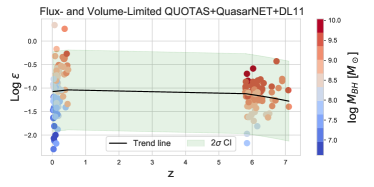
Figure 5: This graph illustrates the relationship between accretion efficiency, redshift, and SMBH mass using the flux- and volume-limited samples from the QUOTAS+QuasarNET+DL11 datasets, along with a trend line indicating the peak of accretion efficiency. A regression fit has been applied to the flux- and volume-limited datasets, clearly showing the peaks of the data, with observed values around $z\sim 2.675$.

What can be understood from the said graphs is that in low redshifts, the mass of the central SMBHs of quasars in the local universe tends to decrease as $z\sim 0.025$. Therefore, SMBHs with closer distance have less mass compared to farther SMBHs.

The situation for the high redshift data is inversely correlated. Therefore, investigating the two datasets of DL11 and QUOTAS+QuasarNET together, the QUOTAS+QuasarNET+DL11 datasets can anticipate a peak where the two trends meet, as can be seen in Fig. 5.

To understand how accretion efficiency behaves over time, it is necessary to compare new and corrected data that have been subjected to flux- and volume-limitations. These restrictions are prominent to ensure that the data is as precise and reliable as possible. In Sec. 6, a deeper delve is made into why these limitations are deemed essential in the context of this study. Despite a more than 50% reduction in the abundance of the data, accretion efficiency shows growth as a function of growing mass. Therefore, the correlation between SMBHs accretion efficiency and SMBHs mass is shown independent of flux- and volume-limitations.

It should be mentioned again that since flux- and volume-limit corrections have little to no effect on data with low redshifts, the plot of flux- and volume-limited for the DL11 dataset is identical to Fig. 3.

Visualizing the results is also essential to understand the data better. In Fig. 5, a regression fit has been applied to the flux- and volume-limited data. This results in a clear indication of the peaks of the data, with values of approximately $z\sim 2.675$ being observed. This peak can serve as a reminder for the redshift range, $z_{SFR}\sim 1-3$, in which the peak of SFR occurs.

As discussed before, SFR shows the amount of mass produced per year in a galaxy. Using the low-mass X-ray binaries (LMXBs) data, White & Ghosh (1998) has reported the SFR peak to be $z\sim 1.5$. Moreover, multiple works such as Atek et al. (2014), Zolotov et al. (2015), and Driver et al. (2018) show that the peak of SFR is at $z\sim 2$, about 3.5 billion years after the Big Bang. To go further into detail of the redshift range of the peak of SFR, Hopkins & Beacom (2006) produced an extensive collection of observations of luminosity density, covering a wide range of redshifts up to $z=6$. Their findings indicate a significant increase in the SFR at low redshifts, reaching its highest point at around $z\simeq 2$ and declining at higher redshifts (Vangioni et al., 2015). Cucciati et al. (2012) reports the Star Formation Rate Density (SFRD) peak to be $z\sim 2$, using the VIMOS-VLT Deep Survey (VVDS). In Jo et al. (2021), for the 1752 objects of the Spitzer COSMOS Legacy survey, the SFRD peak is approximated between $z\sim 2.2-2.4$. Moreso, in Schinnerer et al. (2016), Scoville et al. (2017), and Tacconi et al. (2018) using the data from Main Sequence (MS) galaxies, the peak of SFR is located in $z\sim 1.5-3$. Additionally, according to Reddy et al. (2007), Madau & Dickinson (2014), and Hodge & da Cunha (2020), the redshift in which SFR is at its maximum is thought to be around $z\sim 1-3$. If the target data is increased and more accurate surveys are used, with the condition that they will include all the necessary parameters for calculating the accretion efficiency, the final result will be more precisely finalized. By analyzing this data, a better understanding of how accretion efficiency behaves over time can be obtained, and more accurate predictions about future trends can be made.

By fitting a trend line to the corrected flux- and volume-limited QUOTAS+QuasarNET+DL11 dataset, a new equation is attained,

$$log(\epsilon_{2\sigma})=-0.01621z^{2}+0.08671z-1.07704\pm 0.8505,$$ (11)

As mentioned before, the peak nears the SFR peak much more closely. Note that the $4\sigma$ error bar for the accretion efficiency of the mentioned data is $\epsilon_{4\sigma}\sim 1.7011$. Based on Fig. 5, and the observed peak, the accretion efficiency should be part of the parameters where the downsizing problem must be investigated for. Thus, future works could delve deeper into this concept, focusing on the downsizing process and considering accretion efficiency.

9 Conclusion

In this paper, we have employed datasets containing SMBHs in the center of quasars, using the information of QUOTAS+QuasarNET+DL11 datasets. The QUOTAS+QuasarNET datasets used by projects, such as the QUOTAS and QuasarNET datasets, encompass 37648 high redshift objects, and the DL11 dataset includes 80 PG low redshift quasars. These datasets include essential parameters, such as SMBH mass, bolometric luminosity, optical luminosity, and Eddington luminosity.

Using these parameters, numerous models have been developed to estimate the accretion efficiency for SMBHs, and various previous calculations and simulations have been conducted. However, whether we can accurately make a model to find the dependency of accretion efficiency on redshift and SMBH mass has been questioned. Different methods have been proposed for calculating this parameter, and in this work, we have opted for an approach based on optical luminosity because other methods yield values beyond the feasible range ($0.038<\epsilon<0.42$) for accretion efficiency.

Since there is a need for a comprehensive model to calculate the accretion efficiency in all redshifts, the DL11 low redshift ($z<0.5$) dataset has been used in addition to the QUOTAS+QuasarNET. By fitting the spectra of individual AGNs with the standard thin accretion disk model, it is possible to deduce the absolute accretion efficiency. This dataset provides a robust estimate of the bolometric luminosity as it includes a wide variety of bands, from optical to far-UV and X-rays. These luminosities allow one to ascertain the accretion efficiency of each source.

As a part of the data pre-processing, we have excluded AGNs with RIAF and slim disks. Additionally, in a subsequent data refinement step, we have applied the flux- and volume-limiting corrections to be able to work on the dataset through redshift. The primary focus has been on investigating the evolution of the accretion efficiency over redshift or cosmic time to determine if it follows a discernible pattern.

Given the research conducted by Tabasi et al. (2023) on SMBHs mass, we were intrigued by the possibility of modeling based on redshift. In the mentioned work, they found a peak for SMBH mass evolution through redshift; therefore, we were curious to see whether the accretion efficiency had the same peak or not.

In the QUOTAS+QuasarNET dataset, there is a visible pattern where accretion efficiency rises as the redshift decreases, along with an increase in mass growth. On the other hand, in the DL11 dataset, as redshift increased, both accretion efficiency and mass exhibited growth, leading us to identify a redshift peak between the trends of these two datasets. Subsequently, we have recognized the optimal fit for the flux- and volume-limited QUOTAS+QuasarNET+DL11 dataset. The calculations of this paper begin by examining the correlation between the mass of SMBHs and the accretion efficiency. It is evident from Fig. 2 that SMBHs with a higher mass also have higher accretion efficiency. Nonetheless, the fact that the central SMBHs of quasars are heavier at higher redshifts is evident. Then, an examination is conducted into the correlation between accretion efficiency and redshift. The peak of the accretion efficiency factor is observed with the information of 79 quasars from the DL11 dataset and 76 quasars from the QUOTAS+QuasarNET dataset, after flux- and volume-limiting corrections, as illustrated in Fig. 5.

The redshift peak for the flux- and volume-limited dataset occurred at approximately $z\sim 2.675$. This peak can be a recollection of the SFR peak, which is between $1<z<3$, prompting us to explore potential similarities between this peak and the SFR peak, as well as investigate whether the accretion efficiency could mirror the SFR in AGNs. The peak we have found is closely aligned with existing introduced values by different works, as mentioned in Sec. 8.

It is worth noting that Tabasi et al. (2023) have created a model for SMBHs mass in terms of redshift, and the observed peak has been approximately $z\sim 4.72$. They have also stated that they have not considered SFR in their work. In contrast, our work has used the calculations related to the accretion efficiency for the mentioned result, and it seems that the final peak has automatically considered the SFR, where it has been implemented internally.

Future works can investigate the relationship between the mass of central SMBHs of quasars, SFR, and accretion efficiency. Moreover, a comprehensive and complete model can be achieved by incorporating data from additional surveys, utilizing a larger dataset across all redshifts, and comparing the final models with the newly added data from the JWST dataset. In conclusion, it is critical to underscore the importance of priming any constructed model on empirical evidence; relying on simulation, given the present state of knowledge, would be impractical because an accretion model should be chosen between various models for simulations at the beginning. Meanwhile, none of the models are perfect for all quasars in different redshifts. Thus, more accurate observations are needed to estimate the accretion efficiency reliably. Therefore, the physics behind the accretion of SMBHs lacks a flawless model, which can be improved with a significant increase in data.

10 Data Availability

The code behind the data pre-processing of this article is publicly available on GitHub.

We have used the QUOTAS dataset (Natarajan et al., 2023) in this work, which supports the findings of this study and is publicly available on the Google Kaggle platform and can be found at https://www.kaggle.com/data sets/quotasplatform/quotas.

Table 1: This table represents the flux- and volume-limited QUOTAS+QuasarNET dataset, which has been used in this work.

Object	$z^{a}$	Log $M_{BH}^{b}$ [$M_{\odot}$]	Log $L_{bol}^{c}$ [erg/s]	Log $\lambda_{edd}^{d}$ [erg/s]	Log $L_{opt}^{e}$ [erg/s]	$\epsilon_{opt}^{f}$
SDSS J0005-0006	5.844	8.0	46.67	0.556	45.958	0.011
SDSS J1411+1217	5.854	8.954	47.182	0.114	46.47	0.041
SDSS J1411+1217	5.903	9.204	47.272	-0.046	46.56	0.062
SDSS J1306+0356	6.017	9.23	47.123	-0.222	46.411	0.078
SDSS J1306+0356	6.018	9.462	47.053	-0.523	46.342	0.135
SDSS J1630+4012	6.058	9.23	47.043	-0.301	46.332	0.085
SDSS J0303-0019	6.079	8.699	46.591	-0.222	45.879	0.049
SDSS J1623+3112	6.211	9.342	47.155	-0.301	46.444	0.094
SDSS J1030+0524	6.302	9.301	47.114	-0.301	46.402	0.091
SDSS J1030+0524	6.299	9.38	47.193	-0.301	46.481	0.097
SDSS J0842+1218	6.069	9.462	47.178	-0.398	46.467	0.117
SDSS J0005-0006	5.844	7.778	46.67	0.851	45.958	0.007
SDSS J1411+1217	5.854	8.699	47.182	0.342	46.47	0.024
SDSS J1411+1217	5.903	9.0	47.272	0.176	46.56	0.041
SDSS J1306+0356	6.018	9.23	47.053	-0.222	46.342	0.084
SDSS J1630+4012	6.058	8.954	47.043	-0.097	46.332	0.048
SDSS J0303-0019	6.079	8.477	46.591	0.114	45.879	0.031
SDSS J1623+3112	6.211	9.079	47.155	-0.097	46.444	0.055
SDSS J1030+0524	6.302	9.041	47.114	-0.046	46.402	0.053
SDSS J1030+0524	6.299	9.146	47.193	-0.097	46.481	0.06
SDSS J0842+1218	6.069	9.23	47.178	-0.155	46.467	0.073
SDSS J0002+2550	5.818	9.684	47.296	-0.502	46.584	0.079
SDSS J000825.77-062604.6	5.929	9.157	47.028	0.04	46.272	0.075
SDSS J002806.57+045725.3	5.982	9.59	47.004	-0.541	46.292	0.086
SDSS J003311.40-012524.9	5.978	8.452	46.5	-0.065	45.788	0.027
CFHQS J005006+344522	6.251	9.639	47.257	-0.639	46.494	0.153
CFHQS J022122-080251	6.161	9.207	46.663	-0.658	44.976	0.127
SDSS J0353+0104	6.057	9.066	47.107	-0.25	46.217	0.056
SDSS J0810+5105	5.805	9.537	47.226	-0.426	46.514	0.097
SDSS J083525.76+321752.6	5.902	8.948	46.481	-0.58	45.77	0.05
SDSS J0840+5624	5.816	9.223	46.707	-0.63	45.995	0.066
SDSS J0841+2905	5.954	9.468	47.036	-0.234	46.324	0.115
SDSS J0842+1218	6.069	9.595	47.238	-0.418	46.526	0.104
SDSS J1143+3808	5.8	9.654	47.103	-0.665	46.391	0.107
SDSS J114803.28+070208.3	6.344	9.499	47.136	-0.323	46.408	0.127
SDSS J120737.43+063010.1	6.028	10.038	46.964	-0.922	46.253	0.26
SDSS J124340.81+252923.9	5.842	9.757	47.23	-0.641	46.326	0.201
SDSS J1250+3130	6.138	9.159	47.117	-0.059	46.405	0.057
SDSS J1257+6349	5.992	9.521	46.808	-0.642	46.096	0.12
SDSS J1335+3533	5.87	9.777	47.194	-0.697	46.483	0.143
SDSS J142516.30+325409.0	5.862	9.433	46.981	-0.566	46.269	0.067
SDSS J142738.59+331242.0	6.118	8.838	47.056	-0.038	46.151	0.038
CFHQS J142952.17+554717.6W	6.119	9.282	46.926	-0.47	46.214	0.081
SDSS J1436+5007	5.809	9.665	47.133	-0.646	46.421	0.136
SDSS J1545+6028	5.794	9.213	46.677	-0.65	45.965	0.082
SDSS J1602+4228	6.083	9.553	47.269	-0.282	46.557	0.108
SDSS J160937.27+304147.7	6.146	9.623	46.784	-0.89	46.073	0.11
SDSS J1623+3112	6.254	9.39	47.12	-0.36	46.409	0.083
SDSS J1630+4012	6.066	9.349	46.85	-0.665	46.138	0.093
SDSS J2307+0031	5.9	8.479	46.808	-0.092	45.792	0.024
CFHQS J232914-040324	5.883	8.808	46.363	-0.559	45.637	0.08
PSO J060.5529+24.8567	6.17	9.324	47.149	-0.24	46.437	0.069
PSO J210.4472+27.8263	6.166	9.541	46.962	-0.638	46.25	0.145
PSO J228.6871+21.2388	5.893	9.081	46.732	-0.464	46.02	0.05
PSO J333.9859+26.1081	6.027	9.464	46.899	-0.288	46.187	0.135
SDSS J232908.28-030158.8	6.417	8.398	46.563	0.114	45.851	0.027
CFHQS J005006+344522	6.253	9.415	47.246	-0.208	46.534	0.098
CFHQS J022122-080251	6.161	8.845	46.411	-0.481	45.699	0.081
CFHQS J222901+145709	6.152	8.079	46.49	0.38	45.778	0.015
CFHQS J210054-171522	6.087	8.973	46.703	-0.31	45.991	0.075
SDSS J164121.64+375520.5	6.047	8.38	46.791	0.362	46.079	0.02
CFHQS J005502+014618	5.983	8.38	46.511	0.079	45.799	0.028
VIKING J010953.13-304726.3	6.791	9.124	46.708	-0.538	46.0	0.1
VIKING J030516.92-315056.0	6.614	8.954	46.875	-0.194	46.176	0.056
PSO J167.6415-13.4960	6.515	8.477	46.672	0.086	45.954	0.029
ULAS J1120+0641	7.084	9.393	47.262	-0.244	46.556	0.09
HSC J1205-0000	6.73	9.672	46.556	-1.222	45.845	0.372
PSO J231.6576-20.8335	6.586	9.484	47.276	-0.319	46.568	0.108
PSO J247.2970+24.1277	6.476	8.716	47.248	0.415	46.531	0.024
PSO J323.1382+12.2986	6.588	9.143	46.908	-0.357	46.204	0.081
VIKING J234833.34-305410.0	6.902	9.297	46.633	-0.77	45.954	0.141
ULAS J1120+0641	7.1	9.209	47.174	-0.319	46.462	0.04
VIKING J234833.34-305410.0	6.9	9.322	46.685	-0.745	45.973	0.156
VIKING J010953.13-304726.3	6.7	9.031	46.741	-0.62	46.029	0.055
VIKING J030516.92-315056.0	6.6	9.028	46.932	-0.167	46.22	0.041
Notes: We report accretion efficiency using optical luminosity, bolometric luminosity, and SMBH mass utilizing Eq. (7). a Redshift. b Mass of the SMBH in units of $M_{\odot}$. c Bolometric luminosity in units of erg $s^{-1}$. d Eddington ratio in units of erg $s^{-1}$. e Optical luminosity in units of erg $s^{-1}$. f Accretion efficiency.

Table 2: This table represents the flux- and volume-limited DL11 dataset for low redshift PG quasars.

Object	$z^{a}$	Log $M_{BH}^{b}$ [$M_{\odot}$]	Log $L_{bol}^{c}$ [erg/s]	Log $\lambda_{edd}^{d}$ [erg/s]	Log $L_{opt}^{e}$ [erg/s]	Log $\dot{M}^{f}$ [$M_{\odot}yr^{-1}$]	$\epsilon_{obs}^{g}$
0003 + 158	0.45	9.055	46.92	-0.358	45.87	0.79	0.302
0003 + 199	0.026	7.22	45.13	-0.342	43.91	-0.06	0.034
0007 + 106	0.089	8.561	45.52	-0.972	44.55	-0.42	0.191
0026 + 129	0.145	7.833	46.15	0.053	44.99	0.8	0.05
0043 + 039	0.386	8.952	45.98	-0.648	45.47	0.36	0.091
0050 + 124	0.059	7.238	45.12	0.162	44.41	0.58	0.008
0052 + 251	0.154	8.745	46.06	-0.822	45.0	-0.04	0.282
0157 + 001	0.163	8.006	45.93	-0.261	45.02	0.59	0.049
0804 + 761	0.1	8.352	45.82	-0.3	44.79	0.2	0.093
0838 + 770	0.132	7.992	45.22	-0.493	44.56	0.08	0.031
0844 + 349	0.064	7.759	45.4	-0.479	44.31	-0.01	0.058
0921 + 525	0.035	7.206	44.47	-0.802	43.56	-0.55	0.023
0923 + 129	0.029	7.233	44.53	-0.665	43.58	-0.49	0.023
0923 + 201	0.193	9.094	45.68	-1.134	44.81	-0.47	0.309
0947 + 396	0.206	8.53	46.2	-0.909	45.2	0.19	0.224
1001 + 054	0.161	7.645	45.36	-0.02	44.69	0.59	0.013
1011 - 040	0.058	7.19	45.02	-0.146	44.08	0.17	0.015
1012 + 008	0.186	8.0	45.53	0.0	44.95	0.46	0.026
1022 + 519	0.045	6.94	45.1	-0.6	43.56	-0.36	0.065
1048 - 090	0.346	9.022	46.57	-0.679	45.45	0.3	0.417
1048 + 342	0.167	8.241	45.7	-0.687	44.74	0.02	0.105
1049 - 006	0.36	8.989	46.29	-0.63	45.46	0.34	0.195
1100 + 772	0.312	9.112	46.61	-0.749	45.51	0.29	0.457
1103 - 006	0.423	9.132	46.19	-0.737	45.43	0.21	0.209
1114 + 445	0.144	8.415	45.92	-0.927	44.75	-0.16	0.263
1115 + 407	0.154	7.505	45.59	-0.139	44.58	0.49	0.028
1116 + 215	0.176	8.425	46.27	-0.139	45.31	0.69	0.083
1119 + 120	0.05	7.28	45.18	-0.462	44.01	-0.06	0.038
1121 + 422	0.225	7.856	45.87	-0.232	44.8	0.48	0.054
1126 - 041	0.06	7.598	45.16	-0.434	44.19	-0.02	0.034
1149 - 110	0.049	7.729	44.75	-0.916	43.79	-0.66	0.058
1151 + 117	0.176	8.435	45.43	-0.801	44.65	-0.2	0.095
1202 + 281	0.165	8.462	45.39	-1.053	44.58	-0.38	0.129
1211 + 143	0.081	7.831	46.41	0.051	44.85	0.68	0.117
1216 + 069	0.332	9.0	46.61	-1.0	45.62	0.51	0.282
1226 + 023	0.158	8.876	47.09	-0.012	46.03	1.18	0.182
1229 + 204	0.064	8.004	45.06	-0.804	44.24	-0.35	0.056
1244 + 026	0.048	6.614	44.74	0.235	43.7	0.15	0.009
1259 + 593	0.477	8.738	47.04	-0.085	45.79	0.99	0.245
1302 - 102	0.278	8.749	46.51	-0.08	45.71	0.92	0.087
1307 + 085	0.154	8.541	45.93	-0.651	44.92	0.05	0.166
1309 + 355	0.182	8.155	45.63	-0.421	44.95	0.37	0.04
1310 - 108	0.034	7.759	44.37	-1.183	43.56	-1.0	0.052
1322 + 659	0.168	8.076	45.92	-0.409	44.78	0.27	0.098
1341 + 258	0.086	7.878	44.94	-0.756	44.13	-0.37	0.045
1351 + 236	0.055	8.216	44.57	-1.748	43.93	-1.14	0.112
1351 + 640	0.088	8.656	45.31	-1.058	44.69	-0.38	0.107
1352 + 183	0.151	8.299	45.72	-0.629	44.65	-0.06	0.132
1402 + 261	0.164	7.845	46.07	0.018	44.82	0.63	0.06
1404 + 226	0.098	6.713	45.21	0.232	44.16	0.55	0.01
1411 + 442	0.09	7.874	45.06	-0.535	44.45	0.02	0.025
1415 + 451	0.113	7.797	45.6	-0.579	44.34	-0.06	0.1
1416 - 129	0.129	9.002	45.82	-0.845	44.94	-0.21	0.234
1425 + 267	0.364	9.317	46.35	-1.28	45.55	0.07	0.417
1426 + 015	0.086	8.921	45.84	-1.117	44.71	-0.49	0.479
1427 + 480	0.22	7.978	45.64	-0.344	44.69	0.27	0.051
1435 - 067	0.129	8.3	45.6	-0.412	44.9	0.26	0.048
1440 + 356	0.078	7.335	45.62	-0.013	44.37	0.43	0.034
1444 + 407	0.268	8.158	46.28	-0.122	45.11	0.66	0.091
1501 + 106	0.036	8.482	44.9	-1.172	44.18	-0.79	0.107
1512 + 370	0.371	9.168	47.11	-0.867	45.48	0.2	1.82
1519 + 226	0.136	7.777	45.98	-0.311	44.45	0.18	0.138
1534 + 580	0.03	8.047	44.49	-1.565	43.63	-1.24	0.12
1535 + 547	0.039	7.01	44.34	-0.373	43.9	-0.01	0.005
1543 + 489	0.401	7.844	46.43	0.369	45.27	1.18	0.039
1545 + 210	0.264	9.0	46.14	-1.0	45.29	0.01	0.295
1552 + 085	0.119	7.364	45.04	0.04	44.5	0.56	0.007
1612 + 261	0.131	7.913	45.38	-0.395	44.54	0.15	0.038
1613 + 658	0.129	8.953	45.89	-1.457	44.75	-0.59	0.676
1617 + 175	0.114	8.729	45.44	-0.88	44.63	-0.38	0.145
1626 + 554	0.132	8.371	45.53	-0.94	44.46	-0.4	0.186
1704 + 608	0.372	9.198	46.67	-0.772	45.65	0.38	0.437
2112 + 059	0.46	8.834	46.47	0.116	45.92	1.16	0.046
2130 + 099	0.063	7.805	45.52	-0.367	44.35	0.05	0.065
2209 + 184	0.07	8.601	46.02	-1.353	44.11	-0.98	2.188
2214 + 139	0.066	8.308	45.15	-1.027	44.36	-0.5	0.098
2251 + 113	0.326	8.816	46.13	-0.363	45.6	0.66	0.066
2304 + 042	0.043	8.32	44.49	-1.633	43.67	-1.35	0.155
2308 + 098	0.434	9.372	46.61	-0.936	45.62	0.22	0.537
Notes: We report accretion efficiency using optical luminosity, bolometric luminosity, and SMBH mass. a Redshift. b Mass of the SMBH in units of $M_{\odot}$. c Bolometric luminosity in units of erg $s^{-1}$. d Eddington ratio in units of erg $s^{-1}$. e Optical luminosity in units of erg $s^{-1}$. f Accretion rate, in units of $M_{\odot}yr^{-1}$. g Accretion efficiency.

References

- Abramowicz et al. (1988) Abramowicz, M., Czerny, B., Lasota, J., & Szuszkiewicz, E. 1988, Astrophysical Journal, Part 1 (ISSN 0004-637X), vol. 332, Sept. 15, 1988, p. 646-658. Research supported by Observatoire de Paris and NASA., 332, 646
- Aghamousa et al. (2016a) Aghamousa, A., Aguilar, J., Ahlen, S., et al. 2016a, arXiv preprint arXiv:1611.00036
- Aghamousa et al. (2016b) —. 2016b, arXiv preprint arXiv:1611.00037
- Aghanim et al. (2020) Aghanim, N., Akrami, Y., Ashdown, M., et al. 2020, Astronomy & Astrophysics, 641, A6
- Alam et al. (2015) Alam, S., Albareti, F. D., Prieto, C. A., et al. 2015, The Astrophysical Journal Supplement Series, 219, 12
- Alam et al. (2021) Alam, S., Aubert, M., Avila, S., et al. 2021, Physical Review D, 103, 083533
- Alonso et al. (2016) Alonso, D., Louis, T., Bull, P., & Ferreira, P. G. 2016, Physical Review D, 94, 043522
- Armijo (2012) Armijo, M. M. 2012, Accretion disk theory, Tech. rep.
- Atek et al. (2014) Atek, H., Kneib, J.-P., Pacifici, C., et al. 2014, The Astrophysical Journal, 789, 96
- Banados et al. (2018) Banados, E., Venemans, B. P., Mazzucchelli, C., et al. 2018, Nature, 553, 473
- Bardeen et al. (1972) Bardeen, J. M., Press, W. H., & Teukolsky, S. A. 1972, Astrophysical Journal, Vol. 178, pp. 347-370 (1972), 178, 347
- Begelman (1978) Begelman, M. C. 1978, Monthly Notices of the Royal Astronomical Society, 184, 53
- Begelman et al. (1984) Begelman, M. C., Blandford, R. D., & Rees, M. J. 1984, Reviews of Modern Physics, 56, 255
- Beloborodov (2001) Beloborodov, A. M. 2001, Advances in Space Research, 28, 411
- Best et al. (2024) Best, W. M., Sanghi, A., Liu, M. C., Magnier, E. A., & Dupuy, T. J. 2024, arXiv preprint arXiv:2401.09535
- Beutler et al. (2017) Beutler, F., Seo, H.-J., Saito, S., et al. 2017, Monthly Notices of the Royal Astronomical Society, 466, 2242
- Bian & Zhao (2003) Bian, W.-H., & Zhao, Y.-H. 2003, Publications of the Astronomical Society of Japan, 55, 599
- Blakely & Nikiforakis (2015) Blakely, P., & Nikiforakis, N. 2015, Astronomy & Astrophysics, 583, A90
- Blakeslee et al. (2002) Blakeslee, J. P., Lucey, J. R., Tonry, J. L., et al. 2002, Monthly Notices of the Royal Astronomical Society, 330, 443
- Bondi (1952) Bondi, H. 1952, Monthly Notices of the Royal Astronomical Society, 112, 195
- Bondi & Hoyle (1944) Bondi, H., & Hoyle, F. 1944, Monthly Notices of the Royal Astronomical Society, 104, 273
- Boyle et al. (2000) Boyle, B. J., Shanks, T., Croom, S., et al. 2000, Monthly Notices of the Royal Astronomical Society, 317, 1014
- Brandt et al. (2000) Brandt, W., Laor, A., & Wills, B. J. 2000, The Astrophysical Journal, 528, 637
- Bu & Yang (2019) Bu, D.-F., & Yang, X.-H. 2019, Monthly Notices of the Royal Astronomical Society, 484, 1724
- Bu & Zhang (2023) Bu, Q., & Zhang, S. 2023, arXiv preprint arXiv:2310.20637
- Burke et al. (2021) Burke, C. J., Shen, Y., Blaes, O., et al. 2021, Science, 373, 789
- Busca & Balland (2018) Busca, N., & Balland, C. 2018, arXiv preprint arXiv:1808.09955
- Calvet et al. (1999) Calvet, N., Hartmann, L., & Strom, S. E. 1999, arXiv preprint astro-ph/9902335
- Caroline & Terquem (2007) Caroline, E., & Terquem, L. 2007, in Jets from Young Stars: Models and Constraints (Springer), 103–115
- Chakrabarti (1996) Chakrabarti, S. K. 1996, Physics Reports, 266, 229
- Cheng et al. (2020) Cheng, Y.-T., Chang, T.-C., & Bock, J. J. 2020, The Astrophysical Journal, 901, 142
- Cole (2011) Cole, S. 2011, Monthly Notices of the Royal Astronomical Society, 416, 739
- Conselice et al. (2018) Conselice, C. J., Twite, J. W., Palamara, D. P., & Hartley, W. 2018, The Astrophysical Journal, 863, 42
- Cook et al. (2023) Cook, D., Mazzarella, J., Helou, G., et al. 2023, arXiv preprint arXiv:2306.06271
- Cowie et al. (1996) Cowie, L. L., Songaila, A., Hu, E. M., & Cohen, J. 1996, arXiv preprint astro-ph/9606079
- Croom et al. (2004) Croom, S. M., Smith, R., Boyle, B., et al. 2004, Monthly Notices of the Royal Astronomical Society, 349, 1397
- Cruz-Osorio et al. (2023) Cruz-Osorio, A., Rezzolla, L., Lora-Clavijo, F. D., et al. 2023, Journal of Cosmology and Astroparticle Physics, 2023, 057
- Cucciati et al. (2012) Cucciati, O., Tresse, L., Ilbert, O., et al. 2012, Astronomy & Astrophysics, 539, A31
- Cunningham et al. (2020) Cunningham, T., Tremblay, P.-E., Gentile Fusillo, N. P., Hollands, M., & Cukanovaite, E. 2020, Monthly Notices of the Royal Astronomical Society, 492, 3540
- Czerny (2019) Czerny, B. 2019, Universe, 5, 131
- Czerny et al. (2011) Czerny, B., Hryniewicz, K., Nikołajuk, M., & Sadowski, A. 2011, Monthly Notices of the Royal Astronomical Society, 415, 2942
- Davidson (1976) Davidson, K. 1976, Astrophysical Journal, vol. 207, Aug. 1, 1976, pt. 1, p. 710-712. Research supported by the Alfred P. Sloan Foundation, 207, 710
- Davis & Laor (2011) Davis, S. W., & Laor, A. 2011, The Astrophysical Journal, 728, 98
- Dawson et al. (2016) Dawson, K. S., Kneib, J.-P., Percival, W. J., et al. 2016, The Astronomical Journal, 151, 44
- de Jong et al. (2012) de Jong, R. S., Chiappini, C., & Schnurr, O. 2012, in EPJ Web of Conferences, Vol. 19, EDP Sciences, 09004
- De Lucia & Blaizot (2007) De Lucia, G., & Blaizot, J. 2007, Monthly Notices of the Royal Astronomical Society, 375, 2
- Driver et al. (2018) Driver, S. P., Andrews, S. K., Da Cunha, E., et al. 2018, Monthly Notices of the Royal Astronomical Society, 475, 2891
- Du et al. (2014) Du, P., Hu, C., Lu, K.-X., et al. 2014, The Astrophysical Journal, 782, 45
- Duarte & Mamon (2014) Duarte, M., & Mamon, G. A. 2014, Monthly Notices of the Royal Astronomical Society, 440, 1763
- Ebisawa et al. (1991) Ebisawa, K., Mitsuda, K., & Hanawa, T. 1991, Astrophysical Journal, Part 1 (ISSN 0004-637X), vol. 367, Jan. 20, 1991, p. 213-220., 367, 213
- Eddington (1988) Eddington, A. S. 1988, The internal constitution of the stars (Cambridge University Press)
- Edgar (2004) Edgar, R. 2004, New Astronomy Reviews, 48, 843
- Etherington & Thomas (2015) Etherington, J., & Thomas, D. 2015, Monthly Notices of the Royal Astronomical Society, 451, 660
- Fan (1999) Fan, X. 1999, The Astronomical Journal, 117, 2528
- Fan et al. (2003) Fan, X., Strauss, M. A., Schneider, D. P., et al. 2003, The Astronomical Journal, 125, 1649
- Firmani & Avila-Reese (2010) Firmani, C., & Avila-Reese, V. 2010, The Astrophysical Journal, 723, 755
- Firmani et al. (2010) Firmani, C., Avila-Reese, V., & Rodríguez-Puebla, A. 2010, Monthly Notices of the Royal Astronomical Society, 404, 1100
- Font et al. (1999) Font, J. A., Ibáñez, J. M., & Papadopoulos, P. 1999, Monthly Notices of the Royal Astronomical Society, 305, 920
- Fontanot et al. (2009) Fontanot, F., De Lucia, G., Monaco, P., Somerville, R. S., & Santini, P. 2009, Monthly Notices of the Royal Astronomical Society, 397, 1776
- Fronenberg et al. (2023) Fronenberg, H., Maniyar, A. S., Liu, A., & Pullen, A. R. 2023, arXiv preprint arXiv:2309.07215
- Gaskell & Goosmann (2013) Gaskell, C. M., & Goosmann, R. W. 2013, The Astrophysical Journal, 769, 30
- Gezari (2014) Gezari, S. 2014, Physics Today, 67, 37
- Ghirlanda et al. (2012) Ghirlanda, G., Ghisellini, G., Nava, L., et al. 2012, Monthly Notices of the Royal Astronomical Society, 422, 2553
- Green et al. (1986) Green, R. F., Schmidt, M., & Liebert, J. 1986, Astrophysical Journal Supplement Series (ISSN 0067-0049), vol. 61, June 1986, p. 305-352. Research supported by the California Institute of Technology., 61, 305
- Gregoris (2023) Gregoris, D. 2023, General Relativity and Gravitation, 55, 97
- Hanawa (1989) Hanawa, T. 1989, Astrophysical Journal, Part 1 (ISSN 0004-637X), vol. 341, June 15, 1989, p. 948-954., 341, 948
- He et al. (2022) He, T.-Y., Cai, Z., & Yang, R.-J. 2022, The European Physical Journal C, 82, 1067
- Heinzeller & Duschl (2007) Heinzeller, D., & Duschl, W. 2007, Monthly Notices of the Royal Astronomical Society, 374, 1146
- Hewett et al. (1995) Hewett, P. C., Foltz, C. B., & Chaffee, F. H. 1995, Astronomical Journal (ISSN 0004-6256), vol. 109, no. 4, p. 1498-1521, 109, 1498
- Hodge & da Cunha (2020) Hodge, J. A., & da Cunha, E. 2020, Royal Society Open Science, 7, 200556
- Hopkins & Beacom (2006) Hopkins, A. M., & Beacom, J. F. 2006, The Astrophysical Journal, 651, 142
- Howlett et al. (2012) Howlett, C., Lewis, A., Hall, A., & Challinor, A. 2012, Journal of Cosmology and Astroparticle Physics, 2012, 027
- Ichimaru (1977) Ichimaru, S. 1977, The Astrophysical Journal, 214, 840
- Ilbert et al. (2004) Ilbert, O., Tresse, L., Arnouts, S., et al. 2004, Monthly Notices of the Royal Astronomical Society, 351, 541
- Inoue (2010) Inoue, A. K. 2010, Monthly Notices of the Royal Astronomical Society, 401, 1325
- Izumi (2018) Izumi, T. 2018, Publications of the Astronomical Society of Japan, 70, L2
- Jo et al. (2021) Jo, J. U., Youn, S., Kim, S., et al. 2021, Astrophysics and Space Science, 366, 18
- Katz (1977) Katz, J. 1977, Astrophysical Journal, Part 1, vol. 215, July 1, 1977, p. 265-275., 215, 265
- Kawaguchi et al. (2004) Kawaguchi, T., Aoki, K., Ohta, K., & Collin, S. 2004, Astronomy & Astrophysics, 420, L23
- Kawasaki et al. (2012) Kawasaki, M., Kusenko, A., & Yanagida, T. T. 2012, Physics Letters B, 711, 1
- Khangulyan et al. (2023) Khangulyan, D., Aharonian, F., & Taylor, A. M. 2023, The Astrophysical Journal, 954, 186
- Khesali & Khosravi (2013) Khesali, A., & Khosravi, A. 2013, Astrophysics and Space Science, 348, 143
- Kollmeier et al. (2006) Kollmeier, J. A., Onken, C. A., Kochanek, C. S., et al. 2006, The Astrophysical Journal, 648, 128
- Komossa & Zensus (2014) Komossa, S., & Zensus, J. 2014, Proceedings of the International Astronomical Union, 10, 13
- Kozłowski et al. (2009) Kozłowski, S., Kochanek, C. S., Udalski, A., et al. 2009, The Astrophysical Journal, 708, 927
- Kroupa et al. (2020) Kroupa, P., Subr, L., Jerabkova, T., & Wang, L. 2020, Monthly Notices of the Royal Astronomical Society, 498, 5652
- Lawther et al. (2017) Lawther, D., Vestergaard, M., Raimundo, S., & Grupe, D. 2017, Monthly Notices of the Royal Astronomical Society, 467, 4674
- Li et al. (2005) Li, L.-X., Zimmerman, E. R., Narayan, R., & McClintock, J. E. 2005, The Astrophysical Journal Supplement Series, 157, 335
- Li et al. (2023) Li, P., Liu, Y.-q., & Zhai, X.-h. 2023, Physical Review D, 108, 124022
- Li et al. (2012) Li, Y.-R., Wang, J.-M., & Ho, L. C. 2012, The Astrophysical Journal, 749, 187
- Lipunova et al. (2018) Lipunova, G., Malanchev, K., & Shakura, N. 2018, Accretion Flows in Astrophysics, 1
- Liu & Qiao (2022) Liu, B., & Qiao, E. 2022, Iscience, 25
- Liu et al. (2008) Liu, H., Bai, J., Zhao, X., & Ma, L. 2008, The Astrophysical Journal, 677, 884
- Lora-Clavijo et al. (2015) Lora-Clavijo, F., Cruz-Osorio, A., & Méndez, E. M. 2015, The Astrophysical Journal Supplement Series, 219, 30
- Lora-Clavijo & Guzmán (2013) Lora-Clavijo, F., & Guzmán, F. 2013, Monthly Notices of the Royal Astronomical Society, 429, 3144
- Lorenzin & Zampieri (2009) Lorenzin, A., & Zampieri, L. 2009, Monthly Notices of the Royal Astronomical Society, 394, 1588
- Lyke et al. (2020) Lyke, B. W., Higley, A. N., McLane, J., et al. 2020, The Astrophysical Journal Supplement Series, 250, 8
- Lynden-Bell & Pringle (1974) Lynden-Bell, D., & Pringle, J. E. 1974, Monthly Notices of the Royal Astronomical Society, 168, 603
- Madau & Dickinson (2014) Madau, P., & Dickinson, M. 2014, Annual Review of Astronomy and Astrophysics, 52, 415
- Massara et al. (2021) Massara, E., Ho, S., Hirata, C. M., et al. 2021, Monthly Notices of the Royal Astronomical Society, 508, 4193
- Melia (2019) Melia, F. 2019, Monthly Notices of the Royal Astronomical Society, 489, 517
- Morganson et al. (2012) Morganson, E., De Rosa, G., Decarli, R., et al. 2012, The Astronomical Journal, 143, 142
- Mutch et al. (2013) Mutch, S. J., Croton, D. J., & Poole, G. B. 2013, Monthly Notices of the Royal Astronomical Society, 435, 2445
- Narayan & McClintock (2008) Narayan, R., & McClintock, J. E. 2008, New Astronomy Reviews, 51, 733
- Narayan & Yi (1994) Narayan, R., & Yi, I. 1994, arXiv preprint astro-ph/9403052
- Narayan et al. (1995) Narayan, R., Yi, I., & Mahadevan, R. 1995, Nature, 374, 623
- Natarajan et al. (2023) Natarajan, P., Tang, K. S., McGibbon, R., et al. 2023, The Astrophysical Journal, 952, 146
- Neistein et al. (2006) Neistein, E., Van Den Bosch, F. C., & Dekel, A. 2006, Monthly Notices of the Royal Astronomical Society, 372, 933
- Neri-Larios et al. (2011) Neri-Larios, D., Coziol, R., Torres-Papaqui, J., et al. 2011, arXiv preprint arXiv:1106.1561
- Netzer (2015) Netzer, H. 2015, Annual Review of Astronomy and Astrophysics, 53, 365
- Neugebauer et al. (1987) Neugebauer, G., Green, R., Matthews, K., et al. 1987, Astrophysical Journal Supplement Series (ISSN 0067-0049), vol. 63, March 1987, p. 615-644. NSF-supported research., 63, 615
- Novikov & Thorne (1973) Novikov, I. D., & Thorne, K. S. 1973, Black holes (Les astres occlus), 1, 343
- Pâris et al. (2017) Pâris, I., Petitjean, P., Ross, N. P., et al. 2017, Astronomy & Astrophysics, 597, A79
- Pejcha (2020) Pejcha, O. 2020, Proceedings of the International Astronomical Union, 16, 159
- Pereyra et al. (2006) Pereyra, N. A., Berk, D. E. V., Turnshek, D. A., et al. 2006, The Astrophysical Journal, 642, 87
- Pflamm-Altenburg et al. (2007) Pflamm-Altenburg, J., Weidner, C., & Kroupa, P. 2007, The Astrophysical Journal, 671, 1550
- Piotrovich et al. (2023a) Piotrovich, M., Buliga, S., & Natsvlishvili, T. 2023a, Universe, 9, 175
- Piotrovich et al. (2023b) Piotrovich, M. Y., Shablovinskaya, E., Malygin, E., Buliga, S., & Natsvlishvili, T. 2023b, Monthly Notices of the Royal Astronomical Society, stad2934
- Plotkin et al. (2016) Plotkin, R. M., Gallo, E., Haardt, F., et al. 2016, The Astrophysical Journal, 825, 139
- Quataert (2003) Quataert, E. 2003, Astronomische Nachrichten: Astronomical Notes, 324, 435
- Raimundo et al. (2012) Raimundo, S., Fabian, A., Vasudevan, R., Gandhi, P., & Wu, J. 2012, Monthly Notices of the Royal Astronomical Society, 419, 2529
- Reddy et al. (2007) Reddy, N. A., Steidel, C. C., Pettini, M., et al. 2007, arXiv preprint arXiv:0706.4091
- Redmon & Farhadi (2017) Redmon, J., & Farhadi, A. 2017, in Proceedings of the IEEE conference on computer vision and pattern recognition, 7263–7271
- Rees et al. (1982) Rees, M., Begelman, M., Blandford, R., & Phinney, E. 1982, Nature, 295, 17
- Regan et al. (2019) Regan, J. A., Downes, T. P., Volonteri, M., et al. 2019, Monthly Notices of the Royal Astronomical Society, 486, 3892
- Robson (1996) Robson, I. 1996, Wiley-Praxis series in astronomy and astrophysics
- Rosell et al. (2022) Rosell, A. C., Rodriguez-Monroy, M., Crocce, M., et al. 2022, Monthly Notices of the Royal Astronomical Society, 509, 778
- Ross et al. (2012) Ross, N. P., Myers, A. D., Sheldon, E. S., et al. 2012, The Astrophysical Journal Supplement Series, 199, 3
- Ross et al. (2013) Ross, N. P., McGreer, I. D., White, M., et al. 2013, The Astrophysical Journal, 773, 14
- Rybicki & Lightman (1991) Rybicki, G. B., & Lightman, A. P. 1991, Radiative processes in astrophysics (John Wiley & Sons)
- Schinnerer et al. (2016) Schinnerer, E., Groves, B., Sargent, M., et al. 2016, The Astrophysical Journal, 833, 112
- Schlegel et al. (2009) Schlegel, D., White, M., & Eisenstein, D. 2009, arXiv preprint arXiv:0902.4680
- Schmidt & Green (1983) Schmidt, M., & Green, R. F. 1983, Astrophysical Journal, Part 1 (ISSN 0004-637X), vol. 269, June 15, 1983, p. 352-374., 269, 352
- Schneider et al. (2010) Schneider, D. P., Richards, G. T., Hall, P. B., et al. 2010, The Astronomical Journal, 139, 2360
- Scott et al. (2004) Scott, J. E., Kriss, G. A., Brotherton, M., et al. 2004, The Astrophysical Journal, 615, 135
- Scoville et al. (2017) Scoville, N., Lee, N., Bout, P. V., et al. 2017, The Astrophysical Journal, 837, 150
- Sellwood & Masters (2022) Sellwood, J. A., & Masters, K. L. 2022, Annual Review of Astronomy and Astrophysics, 60, 73
- Shakura & Sunyaev (1973) Shakura, N. I., & Sunyaev, R. A. 1973, Astronomy and Astrophysics, Vol. 24, p. 337-355, 24, 337
- Shang et al. (2005) Shang, Z., Brotherton, M. S., Green, R. F., et al. 2005, The Astrophysical Journal, 619, 41
- Shapiro et al. (1976) Shapiro, S. L., Lightman, A. P., & Eardley, D. M. 1976, Astrophysical Journal, vol. 204, Feb. 15, 1976, pt. 1, p. 187-199., 204, 187
- Shen et al. (2019) Shen, Y., Wu, J., Jiang, L., et al. 2019, The Astrophysical Journal, 873, 35
- Shields (1978) Shields, G. 1978, Nature, 272, 706
- Shukla et al. (2016) Shukla, H., Mellema, G., Iliev, I. T., & Shapiro, P. R. 2016, Monthly Notices of the Royal Astronomical Society, 458, 135
- Skrutskie et al. (2006) Skrutskie, M., Cutri, R., Stiening, R., et al. 2006, The Astronomical Journal, 131, 1163
- Smith (2021) Smith, E. A. 2021
- Somerville et al. (2018) Somerville, R. S., Behroozi, P., Pandya, V., et al. 2018, Monthly Notices of the Royal Astronomical Society, 473, 2714
- Tabasi et al. (2023) Tabasi, S. S., Salmani, R. V., Khaliliyan, P., & Firouzjaee, J. T. 2023, arXiv preprint arXiv:2301.01459
- Tacconi et al. (2018) Tacconi, L. J., Genzel, R., Saintonge, A., et al. 2018, The Astrophysical Journal, 853, 179
- Tago et al. (2010) Tago, E., Saar, E., Tempel, E., et al. 2010, Astronomy & Astrophysics, 514, A102
- Tejeda & Aguayo-Ortiz (2019) Tejeda, E., & Aguayo-Ortiz, A. 2019, Monthly Notices of the Royal Astronomical Society, 487, 3607
- Tempel et al. (2014) Tempel, E., Tamm, A., Gramann, M., et al. 2014, Astronomy & Astrophysics, 566, A1
- Torres (2010) Torres, G. 2010, The Astronomical Journal, 140, 1158
- Trakhtenbrot (2014) Trakhtenbrot, B. 2014, The Astrophysical Journal Letters, 789, L9
- Trump et al. (2009) Trump, J. R., Impey, C. D., Kelly, B. C., et al. 2009, The Astrophysical Journal, 700, 49
- Trump et al. (2011) —. 2011, Astrophysical Journal, 733, 60
- Turner & Gott III (1976) Turner, E. L., & Gott III, J. R. 1976, Astrophysical Journal, Suppl. Ser., Vol. 32, p. 409-427, 32, 409
- Vangioni et al. (2015) Vangioni, E., Olive, K. A., Prestegard, T., et al. 2015, Monthly Notices of the Royal Astronomical Society, 447, 2575
- Villar et al. (2011) Villar, V., Gallego, J., Pérez-González, P. G., et al. 2011, The Astrophysical Journal, 740, 47
- Wang et al. (2017) Wang, Y., Xu, L., & Zhao, G.-B. 2017, The Astrophysical Journal, 849, 84
- White & Ghosh (1998) White, N. E., & Ghosh, P. 1998, The Astrophysical Journal, 504, L31
- Wielgus et al. (2015) Wielgus, M., Kluźniak, W., Sadowski, A., Narayan, R., & Abramowicz, M. 2015, Monthly Notices of the Royal Astronomical Society, 454, 3766
- Xu et al. (2023) Xu, K., Jing, Y., Zhao, G.-B., & Cuesta, A. J. 2023, Nature Astronomy, 7, 1259
- Xu & Stone (2019) Xu, W., & Stone, J. M. 2019, Monthly Notices of the Royal Astronomical Society, 488, 5162
- York et al. (2000) York, D. G., Adelman, J., Anderson Jr, J. E., et al. 2000, The Astronomical Journal, 120, 1579
- Yuan & Narayan (2004) Yuan, F., & Narayan, R. 2004, The Astrophysical Journal, 612, 724
- Yuan & Narayan (2014) —. 2014, Annual Review of Astronomy and Astrophysics, 52, 529
- Zhang & Lu (2020) Zhang, F., & Lu, Y. 2020, The Astrophysical Journal, 902, 52
- Zhang & Lu (2017) Zhang, X., & Lu, Y. 2017, Science China Physics, Mechanics & Astronomy, 60, 1
- Zhao et al. (2019) Zhao, G.-B., Wang, Y., Saito, S., et al. 2019, Monthly Notices of the Royal Astronomical Society, 482, 3497
- Zhou et al. (2017) Zhou, H., Wang, T., Yuan, W., et al. 2017, VizieR Online Data Catalog, J
- Zimmerman et al. (2005) Zimmerman, E., Narayan, R., McClintock, J., & Miller, J. 2005, The Astrophysical Journal, 618, 832
- Zolotov et al. (2015) Zolotov, A., Dekel, A., Mandelker, N., et al. 2015, Monthly Notices of the Royal Astronomical Society, 450, 2327