Interface Modes in Honeycomb Topological Photonic Structures with Broken Reflection Symmetry††thanks: J. Lin was partially supported by the NSF grant DMS-2011148, and H. Zhang was partially supported by Hong Kong RGC grant GRF 16304621 and NSFC grant 12371425
Abstract
In this work, we present a mathematical theory for Dirac points and interface modes in honeycomb topological photonic structures consisting of impenetrable obstacles. Starting from a honeycomb lattice of obstacles attaining -rotation symmetry and horizontal reflection symmetry, we apply the boundary integral equation method to show the existence of Dirac points for the first two bands at the vertices of the Brillouin zone. We then study interface modes in a joint honeycomb photonic structure, which consists of two periodic lattices obtained by perturbing the honeycomb one with Dirac points differently. The perturbations break the reflection symmetry of the system, as a result, they annihilate the Dirac points and generate two structures with different topological phases, which mimics the quantum valley Hall effect in topological insulators. We investigate the interface modes that decay exponentially away from the interface of the joint structure in several configurations with different interface geometries, including the zigzag interface, the armchair interface, and the rational interfaces. Using the layer potential technique and asymptotic analysis, we first characterize the band-gap opening for the two perturbed periodic structures and derive the asymptotic expansions of the Bloch modes near the band gap surfaces. By formulating the eigenvalue problem for each joint honeycomb structure using boundary integral equations over the interface and analyzing the characteristic values of the associated boundary integral operators, we prove the existence of interface modes when the perturbation is small.
Keywords: Interface modes, Honeycomb structure, Helmholtz equations, Dirac points, Topological photonics
MSC:35P15, 35Q60, 35J05, 45M05
1 Introduction and outline
1.1 Background and motivation
Photonic and phononic materials with band gaps can be used to localize and confine waves, which have wide applications in the transportation and manipulation of wave energy [45, 50]. In a gapped photonic or phononic crystal, a localized wave mode with frequency in the band gap can be created by introducing a local perturbation in the periodic structure, such as a point or line defect [45]. Such a wave mode is called a defect mode and it is confined near the defect. Mathematically, a defect mode and its frequency correspond to an eigenpair of a locally perturbed periodic operator for the acoustic wave equation or Maxwell’s equations. The existence of point defect modes and line defect modes was proved in [4, 5, 13, 14, 37, 36, 46, 69] for several different configurations of periodic acoustic and electromagnetic media, including the periodic dielectric media, high contrast media, and bubbly media, etc. Besides the deterministic approaches, random media also allows for wave localization. One well-known strategy is the Anderson localization, wherein a periodic medium is randomly perturbed in the whole spatial domain [31, 32, 35, 67].
The recent development in topological insulators (cf. [42, 12, 63]) opens up new avenues for wave localization and confinement in photonic and phononic materials. The concept of topological phases for classical waves was proposed in the seminal work [23], when it was realized that topological band structures are a ubiquitous property of waves for periodic media, regardless of the classical or quantum nature of the waves. Therefore, the concepts in topological insulators can be parallelly extended to periodic wave media, and remarkably, extensive research work has been sparked in pursuit of topological acoustic, electromagnetic, and mechanical insulators to manipulate the classical wave in the same way as solids modulating electrons [48, 57, 59, 61, 75]. Briefly speaking, there are mainly two strategies to realize topological structures for classical waves. The first strategy mimics the quantum Hall effect in topological insulators using active components to break the time-reversal symmetry of the system [49, 73]. The second strategy relies on an analog of the quantum spin Hall effect or quantum valley Hall effect, and it uses passive components to break the spatial symmetry of the system [58, 74].
Wave localization in topological structures is achieved by gluing together two periodic media with distinct topological invariants. The topological phase transition at the interface of two media gives rise to the so-called interface modes, which propagate parallel to the interface but localize in the direction transverse to the interface. Recently there has been intensive mathematical research investigating the interface modes in topological insulators from different perspectives. In particular, the existence of interface modes was proved in [20, 26, 27, 54] for the Schrödinger operator and several other elliptic operators, wherein the interfaces are modeled by smooth domain walls. In addition, the spectra of interface modes are closely related to the topological nature of the bulk media. In general, the net number of interface modes is equal to the difference of the bulk topological invariants across the interface, which is known as the bulk-edge correspondence [42, 61]. We refer to [9, 10, 22, 21, 43] for the studies of the bulk-edge correspondence in discrete electron models and [17, 19] for the bulk-edge correspondence in several elliptic PDE models.
In this work, we study the interface modes in a joint honeycomb photonic structure, where two periodic lattices separated by an interface are obtained by perturbing a honeycomb lattice with Dirac points differently. Such perturbations break the reflection symmetry of the system, as a result, they annihilate the Dirac points and generate two structures with different topological phases. This mimics the quantum valley Hall effect in topological insulators [58, 74]. A one-dimensional joint structure with a similar setup was investigated [56, 70] using the transfer matrix method and the oscillatory theory for Sturm-Liouville operators. In contrast to the studies of interface modes in [20, 26, 27, 54], where two bulk media are “connected” adiabatically over a length scale that is much larger than the period of the structure to form a joint photonic structure and the interface is modeled by a smooth domain wall extending to the whole spatial domain, we consider more realistic models where two periodic media are connected directly such that the medium coefficient attains a jump across the interface. Therefore, we have to address the new challenges in the spectral analysis brought by the discontinuities of coefficients in the PDE model. Beyond that, we consider the model with more general shapes of the interface that separates two bulk media. The goal of this work is to develop a mathematical framework based on a combination of layer potential theory, asymptotic analysis, and the generalized Rouché theorem to examine the existence of the interface modes in such settings. The mathematical framework can be extended to study localized modes in other contexts.
1.2 Outline
1.2.1 The honeycomb lattice and Dirac points
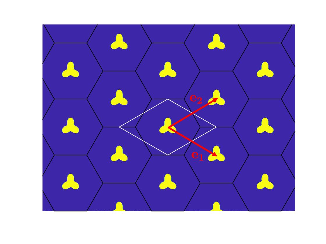
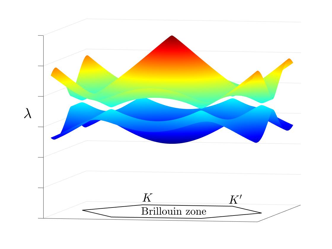
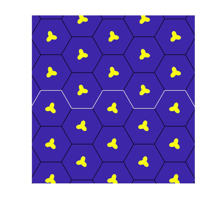
We start from a honeycomb lattice consisting of a two-dimensional array of impenetrable obstacles and examine the existence of Dirac points in the band structure of the lattice. A schematic plot of the periodic structure and its band structure is shown in Figure 1.1. The honeycomb lattice is a natural choice for the photonic structure, as it attains the desired symmetry to create Dirac points over the vertices of the Brillouin zone [11, 24].
Dirac points refer to conical intersections of two dispersion surfaces in the band structure. They are the degenerate points in the spectrum where the topological phases of the material may change. More specifically, at a Dirac point , the eigenspace of the associated partial differential operator spans a two-dimensional space. In addition, the two dispersion surfaces forming the Dirac point attain the following expansion
| (1.1) |
wherein denotes the slope of the linear dispersion relation near the Dirac point. Due to the surging interest in topological insulators, Dirac points were investigated for a broad class of PDE operators recently, especially for the Schrödinger operator over the honeycomb lattice, the Helmholtz operator with high-contrast medium and resonant bubbles, etc [3, 15, 24, 11, 29, 53, 54]. In general, Dirac points exist at the vertices of the Brillouin zone when the medium coefficients in the honeycomb lattice attain suitable symmetry, such as inversion and -rotation symmetry, horizontal reflection and -rotation symmetry, etc. The degeneracy at a Dirac point can be deduced from the representation of the relevant symmetry group, and the conical shape of the dispersion relation is obtained from its invariance under the rotation symmetry [11].
In this work, we apply the boundary integral equation method to show the existence of Dirac points for the first two bands at the vertices of the Brillouin zone, assuming that the shape of each obstacle in the lattice attains -rotation symmetry and horizontal reflection symmetry as shown in Figure 1.1. The existence of Dirac points for obstacles with other symmetries can be examined similarly using this method.
1.2.2 The perturbed honeycomb lattices: spectral gap and topological phase
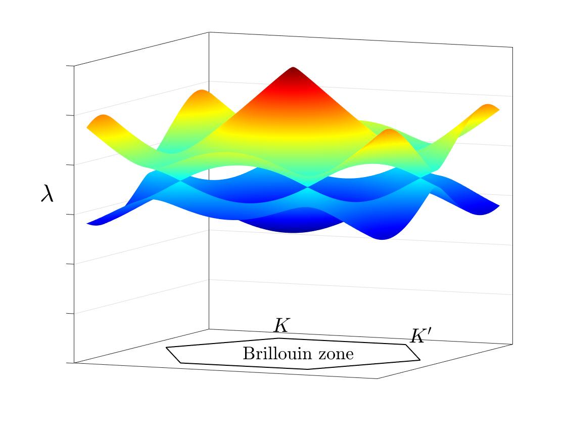
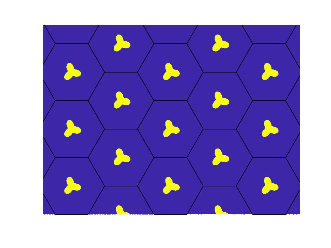
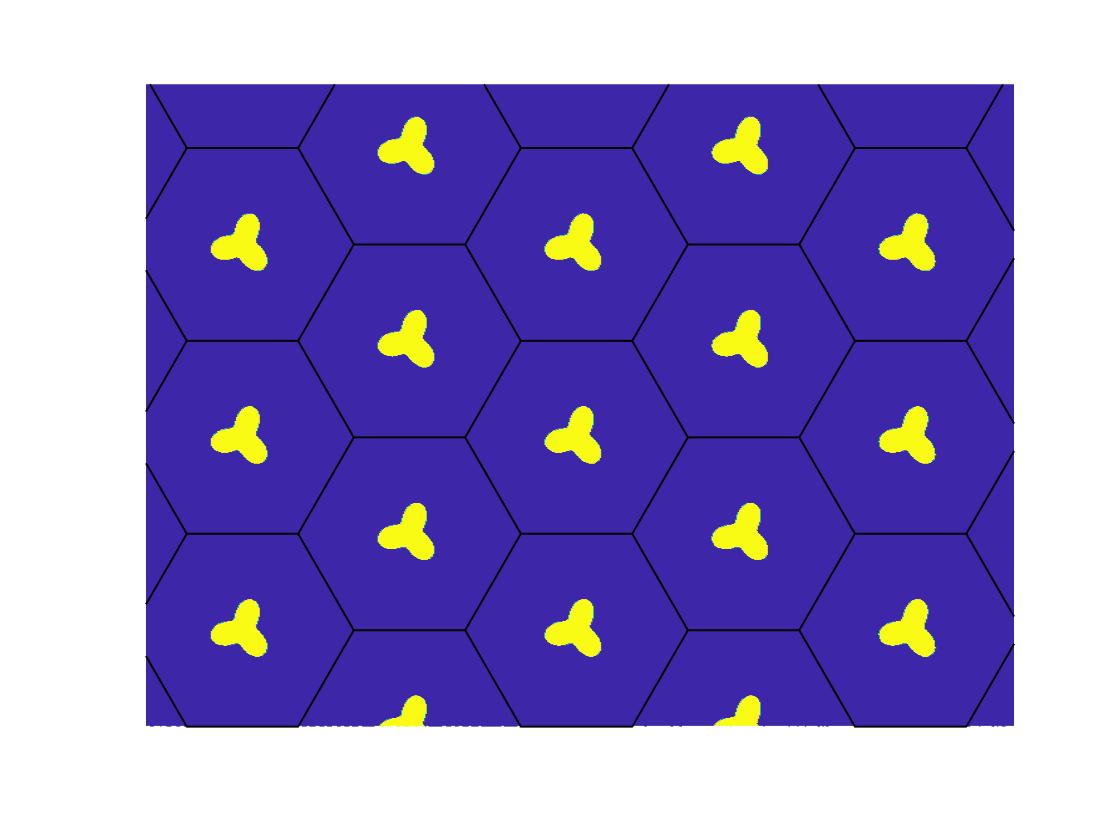
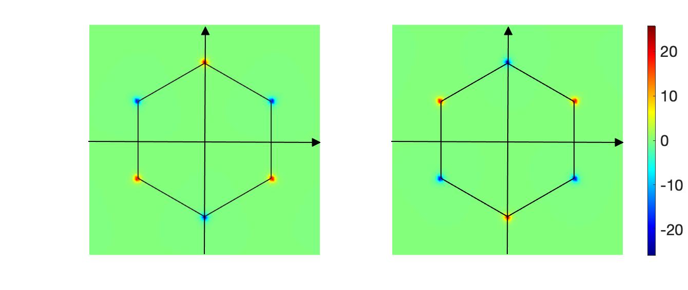
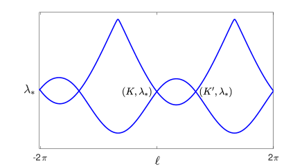
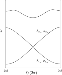
We then break the spatial reflection symmetry of the honeycomb lattice by rotating the obstacles in opposite directions to obtain two photonic structures in Figure 1.2, which will create spectral gaps at the Dirac point as shown in Figure 1.3 so that wave propagation is prohibited for frequencies located in the gap interval. We carry out the asymptotic analysis for the spectrum of each perturbed periodic operator using the layer potential technique and prove that a spectral gap is opened at the Dirac point when the perturbation is small. Furthermore, we prove that the eigenspaces at the band edges are swapped for the two perturbed periodic operators, which demonstrates the topological phase transition of the medium at the Dirac point. The topological phase difference between the two lattices can also be manifested through the Berry phase, which describes the phase evolution of eigenfunctions in the momentum space [8]. As demonstrated in Figure 1.4, the Berry curvatures associated with the first bands of the two perturbed lattices attain opposite values.

1.2.3 Interface modes in the joint honeycomb lattice
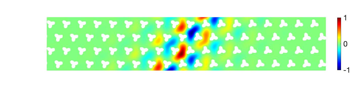
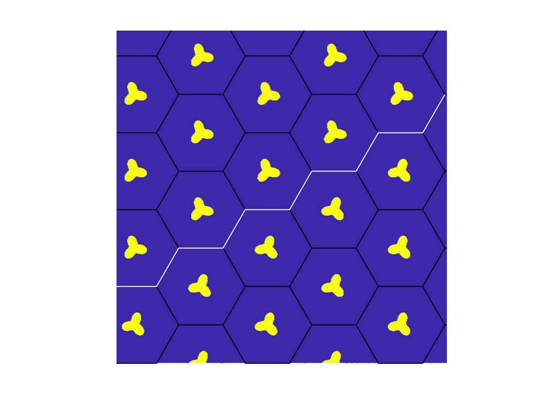
Finally, we investigate the interface modes for the joint photonic structure formed by gluing the two perturbed honeycomb lattices together. The interface modes propagate parallel to the interface of the two media but decay along the direction perpendicular to the interface (cf. Figure 1.5). We consider the PDE operators for several configurations of joint photonic structures attaining different interface geometries, including the zigzag interface, the armchair interface, and the rational interfaces. The configurations of the joint structure with the zigzag and armchair interface are shown in Figure 1.6. We prove the existence of interface modes for the joint structures for each scenario, with the corresponding eigenfrequencies located in the common band gap of the two perturbed media enclosing the Dirac point. To address the sharp discontinuity of the medium coefficient across the interface, we set up a matching condition for the wave field at the interface using integral equations and investigate the characteristic values using the generalized Rouché Theorem in Gohberg-Sigal theory [40, 2]. The method was applied to study the interface modes bifurcated from Dirac points in the topological waveguide structure recently [64] and can be employed to study interface modes in photonic structures with piecewise constant media in a general context.
1.3 Notations
Honeycomb lattice
, : the honeycomb lattice and its dual lattice.
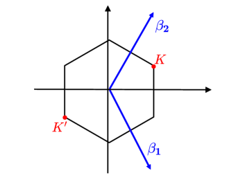
, : high symmetry points in the Brillouin zone.
.
: the fundamental cell of the honeycomb lattice for the zigzag interface.
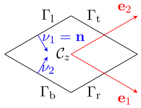
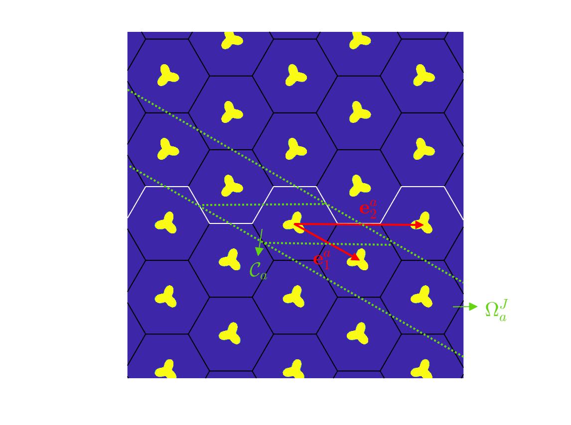
, : generating vectors of the honeycomb lattice with the fundamental cell .
, , , , the left, right, top and bottom sides of . See Figure 2.1.
, : unit normal to and . See Figure 2.1.
, : generating vectors of the dual lattice with .
: the fundamental cell of the honeycomb lattice for the armchair interface.
, : generating vectors of the honeycomb lattice with the fundamental cell .
, : generating vectors of the dual lattice with .
: the reference inclusion with required symmetries.
.
with a sufficiently small .
: the domain obtained by rotating by an angle of counterclockwise.
Layer potentials defined over the inclusion boundary
: single layer potential with Green function for free space Laplacian on , see (3.19).
: single layer potential with quasiperiodic Green function for Helmholtz equation on , see (3.4).
: single layer potential with quasiperiodic Green function for Helmholtz equation on , where represents the orientation, see (4.1).
Infinite strips for joint honeycomb structures
: the infinite strip for the joint honeycomb structure with a zigzag interface.
: the domain of inclusions located in for the joint honeycomb with the zigzag interface.
.
: the zigzag interface for the joint honeycomb structure.
: the top and bottom boundaries of the domain .
: the infinite strip for the joint honeycomb structure with an armchair interface.
: the domain of inclusions located in for the joint honeycomb with the armchair interface.
.
: the armchair interface restricted on .
: the top and bottom boundaries of .
, , .
Energies and modes
, : Bloch modes with quasimomentum at the Dirac point energy . See Theorem 2.1.
: dispersion energies that are numbered from small to large.
: Bloch modes at energy .
: dispersion energies that are smooth along .
: Bloch modes at energy that are smooth along .
, , and : abbreviations of , , and . See
Section 5.1.
, see (7.2)
,
.
Green functions
: quasi-periodic Green function for the Helmholtz equation in ; see (3.1).
:
Green function for the Helmholtz equation in that is quasiperiodic in , see (5.25).
Layer potentials over the interface of the joint honeycomb lattice
, , , , : layer potentials over interface , with the kernel .
, , , : matrix operators with layer potentials over with the kernel .
,
, , , and : layer potentials over , with kernel .
: matrix operator with layer potentials over with kernel .
2 Main results
The first main result of this work is the existence and asymptotic analysis of Dirac points for a family of honeycomb lattices of impenetrable obstacles with Dirichlet boundary conditions. We assume that the shape of each obstacle in the honeycomb lattice attains -rotation symmetry and horizontal reflection symmetry. The second main result is the existence and the number of interface modes for a joint photonic structure formed by gluing two lattices perturbed from the honeycomb lattice attaining Dirac points along an interface. Our results cover the case of a zigzag interface, an armchair interface, and a rational interface. These interface modes are quasi-periodic along the direction of the interface but decay in the direction transverse the interface direction. We also derive the dispersion relation of the interface modes with respect to the quasi-momentum along the interface.
2.1 The honeycomb lattice of impenetrable obstacles
As illustrated in Figure 1.1, an infinite array of impenetrable obstacles are arranged periodically over the honeycomb lattice
wherein the lattice vectors
In what follows, without loss of generality, we assume that the lattice constant . Let
| (2.1) |
be the fundamental cell of the lattice. Let be a connected smooth domain that is invariant under the -rotation transform and the horizontal reflection transform given by
| (2.2) |
Denote the scaled inclusion for .
Let
be the reciprocal lattice, where the reciprocal lattice vectors
| (2.3) |
satisfy , . The hexagon-shaped fundamental cell in , or the Brillouin zone, is denoted by as shown in Figure 2.1 (right). The high symmetry points located at the vertices of the Brillouin zone are given by
2.2 Dirac points for the honeycomb lattice
Following the Floquet-Bloch theory [51], for each , we consider the following eigenvalue problem:
| (2.4) | |||||
For each , the eigenvalues can be ordered by . As varies in the Brillouin zone , one obtains the band structure of the honeycomb lattice.
We define the -vicinity of :
| (2.5) |
where is a complex number defined by (3.22). The main results regarding the Dirac points at and are stated below.
Theorem 2.1.
If Assumption 3.2 holds, then for sufficiently small but nonzero, there exists a Dirac point at in the band structure of the honeycomb lattice with . The dispersion surface near takes the form
| (2.6) |
where the slope of the Dirac cone is
| (2.7) |
In addition, the basis of the eigenspace at the Dirac point can be chosen as and that satisfy
| (2.8) |
in which .
Remark 2.2.
Recall that and defined in (2.2) denote the -rotation operation and the horizontal reflection operation acting on vectors in . Here and henceforth, for convenience of notation, we also use and to denote the rotation and reflection operators acting on functions. The meaning of the notations should be clear in the context, depending on whether they are applied to vectors or functions.
Remark 2.3.
In this work, we only prove the existence of Dirac points for the first two bands and when . It can be shown that Dirac points also exist for higher bands and for not small. This is not the focus of this work and will be reported separately elsewhere.
Corollary 2.4.
For , is also a Dirac point with the corresponding eigenspace spanned by
| (2.9) |
which attain the following symmetry relations:
| (2.10) |
2.3 Band-gap opening at Dirac points
The existence of Dirac points as established in the previous subsection is due to the -rotation symmetry and the horizontal reflection symmetry of the lattice structure. Under suitable perturbations that break one of these symmetries, the Dirac points will disappear and a bandgap can be opened therein. We show that this is indeed the case when the obstacles in the honeycomb lattice are rotated to their centers with an angle of (cf. Figure 1.2) so that the horizontal reflection symmetry of the lattice structure is broken.
In subsequent analysis, we fix by fixing a small enough such that Theorem 2.1 holds for . Denote by the domain obtained by rotating by an angle of counterclockwise. We consider the following eigenvalue problem for each :
| (2.11) |
Theorem 2.5.
Theorem (2.5) can be concluded from Proposition 4.3 with . From the symmetry of the lattice, similar expansions hold for near and near . In view of (2.12), when , there holds for near , thus a spectral gap is opened. The expansion (2.13) demonstrates the swap of the eigenspace at when the obstacles are rotated with the opposite rotation parameter .
Remark 2.6.
The assumption that can be verified numerically for the structure considered in this work.
2.4 Interface modes for the joint photonic structure along a zigzag interface
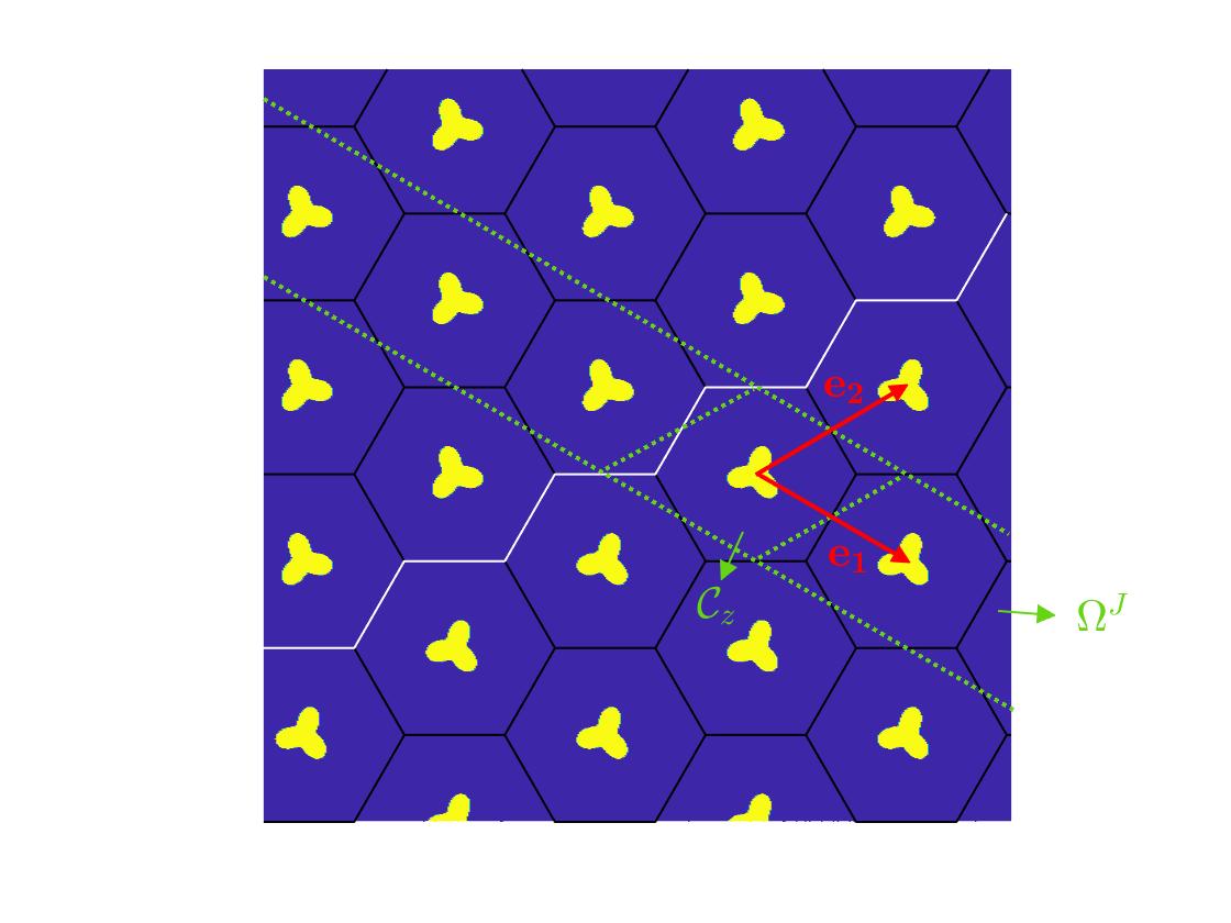
We investigate interface modes for the joint photonic structure with the zigzag interface shown in Figure 2.2. The obstacles are rotated with an angle of and about the origin respectively for the semi-infinite honeycomb lattice on the left and right side of the interface.
Note that the direction of the interface is parallel to . Employing the Floquet theory along , we can restrict our studies to the infinite strip , which is a fundamental period of the joint photonic structure along the interface direction. Inside the strip , the region occupied by the inclusions is denoted by
and the region exterior to the inclusions is denoted by . We also denote the lower boundary of the infinite strip by , then the upper boundary of the strip is . The normal direction on is .
An interface mode for the joint photonic structure solves the following spectral problem:
| (2.14) | |||||
In the above, is the quasi-momentum of the interface modes along the interface, and is normal derivative to .
We first focus on interface modes with the quasi-momentum by projecting the Bloch wave vector onto the direction of the interface . Namely, we investigate the interface modes bifurcated from the Dirac point . The interface modes with other quasi-momenta will be discussed in Section 2.6. To this end, we introduce the following function space
| (2.15) | ||||
Then an interface mode satisfies
| (2.16) |
Assumption 2.7 (The no-fold condition along the direction ).
Remark 2.8.
The above no-fold condition holds for the configuration of the periodic structures considered in this work. Indeed, the first two bands of the spectral problem (2.4) touch at the Dirac point . Moreover, the energy is the maximum of the eigenvalues for the first band and the minimum of the eigenvalues for the second band. This can be rigorously proved when the inclusion size is small by using the layer potential technique and asymptotic analysis. The general case, when is not necessarily small, is beyond the scope of this work. Instead, we demonstrate numerically the no-fold conditions in Figure 2.3 that are used in Theorems 2.9 and 2.12, wherein and respectively.
Theorem 2.9.
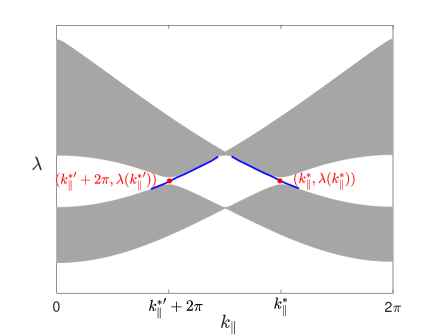
Let Assumption 2.7 hold along the reciprocal lattice vector . Let and be the two constants defined in (4.8) and assume that . Let be an arbitrary constant in . For sufficiently small positive , there exists a unique interface mode satisfying (2.16) with the corresponding eigenvalue . In addition, the interface mode decays exponentially as .
Define the quasi-momentum . By the time-reversal symmetry of the differential operator, the following corollary is a direct consequence of Theorem 2.9.
Corollary 2.10.
Remark 2.11.
Numerical experiment demonstrates that the interface mode persists for not small. This will be analyzed rigorously in the future work.
2.5 Interface modes along an armchair interface
We consider interface modes for the joint photonic structure with an armchair interface as shown in Figure 2.4. The inclusions above the interface are rotated to their centers with an angle of , while the ones below are roated with an angle of . Note that the direction of the interface is along the axis, we rewrite the honeycomb lattice equivalently as
in which the lattice vectors are given by
| (2.17) |
Correspondingly, the fundamental periodic cell is
| (2.18) |
and the reciprocal lattice vectors are
We assume that the inclusions and are strictly included in the cell . Similar to the zigzag interface, we introduce the infinite-strip domain as the fundamental period for the joint photonic structure, which consists of the inclusions and their complement .
We now investigate the interface modes bifurcated from the Dirac point that propagate along the interface direction with the quasi-momentum . Correspondingly, we define the function space
| (2.19) | ||||
Here is the lower boundary of the strip . Then an interface mode with the quasimomentum and energy solves
| (2.20) |
Note that the quasi-momenta satisfying lies on the line for . We have the following results similar to Theorem 2.9 for the spectral problem (2.20).
Theorem 2.12.
Let Assumption 2.7 hold along the reciprocal lattice vector . Let and be the two constants defined in (4.8) and assume that . Let be an arbitrary constant in . For sufficiently small positive , there exist exactly two interface modes with , with the corresponding eigenvalues . In addition, both interface modes decay exponentially as .
2.6 Dispersion relations of the interface modes
We consider interface modes with quasi-momentum near or . In particular, we derive the leading order of the dispersion relation for the interface modes along a zigzag or armchair interface for near or . The dispersion curve over the whole Bloch interval for both configurations are shown in Figure 2.5.
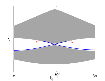
Theorem 2.13.
Theorem 2.14.
Let the assumptions in Theorem 2.12 hold and be an arbitrary constant in . If is sufficiently small and , the eigenvalues of the two interface modes along the armchair interface are .
2.7 Interface modes along rational interfaces
We extend the previous studies to interface modes along a rational interface separating two honeycomb photonic structures. A rational interface is a line with a direction
| (2.21) |
where and are relatively prime integers. When and are relatively prime, there exist , such that and
Therefore, the vectors
| (2.22) |
generate the honeycomb lattice. Correspondingly, the reciprocal vectors
| (2.23) |
generate the dual lattice.
We call an interface direction of the zigzag type if the dual slice intersects with but not with , and is of armchair if the slice intersects with both and . A straightforward calculation shows that if and only if for some .
Definition 2.15.
The direction is called a rational if and are relatively prime integers. The rational interface is of zigzag type if for all , and is of armchair type if for some .
Let the inclusion and all of its rotations be compactly supported in the cell . We prove that the analog of Theorem 2.9 - Theorem 2.14 holds in the case of rational interfaces for the zigzag and armchair types. More specifically,
Denote
| (2.24) |
wherein
| (2.25) |
Then if the rational interface is of zigzag type, we have the following theorem.
Theorem 2.16.
Let be a rational edge of zigzag type and let Assumption 2.7 hold along the reciprocal lattice vector . Let and be the two constants defined in (4.8) and assume that . Let be an arbitrary constant in . If is sufficiently small, then
-
(i)
There exists a unique interface mode along the interface, with the quasi-momentum and the eigenvalue ).
-
(ii)
For , the dispersion relation for the interface mode adopts the expansion .
If the rational interface is of armchair type, we have the following theorem.
Theorem 2.17.
Let be a rational edge of armchair type and let Assumption 2.7 hold along the reciprocal lattice vector . Let and be the two constants defined in (4.8) and assume that . Let be an arbitrary constant in . If is sufficiently small, then
-
(i)
There exist exactly two interface modes along the interface, with the quasi-momentum and the eigenvalues .
-
(ii)
For , the dispersion relations for the interface modes adopt the expansions .
2.8 Extension of results to other settings
We note that the method and framework developed in this paper can be extended to other settings:
-
(1)
There are multiple inclusions in one periodic cell;
-
(2)
The inclusions are penetrable such that the medium coefficient is piecewise constant;
-
(3)
The topological phase transition is induced by perturbations that break either the inversion symmetry or the time-reversal symmetry.
3 Dirac points for the honeycomb lattice
In this section, we prove Theorem 2.1 regarding the Dirac points by the layer potential technique.
3.1 Integral equation formulation
In this subsection, we formulate the spectral problem for the honeycomb structure by using boundary integral equations. For each , let be the quasi-periodic Green function over the honeycomb lattice that solves
| (3.1) |
Define the single-layer potential
wherein the density function . Then it can be shown that solves the eigenvalue problem (2.4) if and only if solves the following boundary integral equation:
| (3.2) |
Define . Then a point belongs to the dispersion surface of the honeycomb lattice if and only if the triple solves the integral equation
| (3.3) |
where the single-layer integral operator
| (3.4) |
In the rest of this section, we investigate the characteristic values of the integral operator when .
3.2 Symmetry of the integral operator
In this subsection, we establish symmetry properties of the integral operator . Note that the Green function satisfying (3.1) can be represented by the lattice sum (cf. [2])
| (3.5) |
where is the zero-order Hankel function of the first kind. More precisely,
| (3.6) |
where
and is the Euler constant. The Green function also attains the following spectral decomposition (cf. [2]):
| (3.7) |
wherein represents the area of the fundamental cell .
Recall that is the Sobolev space of order defined on . Note that the transformation is unitary and it attains three eigenvalues , and , where . Define
| (3.8) |
These subspaces are pairwise orthogonal under the inner product and there holds
In addition, using the relation , we have .
Define
| (3.9) |
A straightforward calculation shows that
| (3.10) |
Here we have used
| (3.11) |
and
| (3.12) |
Lemma 3.1.
Proof.
and
In the above, we have used , and . The relation
can be shown similarly using the relation .
Statement (ii) follows from the standard layer potential theory; see for instance [2].
Statement (iii) is a consequence of the relation , which implies if and only if . ∎
3.3 Dirac points in the lowest two bands
In this subsection, we establish the existence of Dirac points in the lowest two bands. In view of (3.5) and (3.7), when , the Green function attains singularities around and for each . The singularity for the former arises naturally when the source point and the target point overlap, while the latter occurs at special frequencies when the spectral decomposition (3.7) is not well-defined.
As to be shown below, the Dirac point at with the lowest energy appears when , where attains the smallest norm among all lattice points in . A straightforward calculation shows that
in which
We now perform asymptotic expansion of the operator for . To this end, we derive the expansion for Green’s function when is small. For simplicity we consider instead, since . From the above discussions, the Green function attains singularities when or for some , and those terms contributing to the singularities are the leading-order terms in the expansion of .
From the lattice sum (3.5), the singularity at arises from the term with . Using the expansion
we define the leading-order term by and the remainder by as follows:
| (3.13) | ||||
From the spectral decompostion (3.7), the singularity at arises from the terms
We consider in the -neighborhood of , namely, where is defined in (2.5). Correspondingly, we define the leading-order term by and the remainder by as follows:
| (3.14) | ||||
Finally, the smooth term in the Green’s function is denoted by
| (3.15) |
Using the above expansions for the Green’s function, we obtain the decomposition for the integral operator :
| (3.16) |
where the leading-order integral operator is
| (3.17) |
and the remainder operator is
| (3.18) |
Let be the single layer potential associated with the Laplace operator in free space defined by
| (3.19) |
Assumption 3.2.
The operator is invertible.
Remark 3.3.
Remark 3.4.
The operator defined in (3.19), and the operators and commute with and .
Lemma 3.5.
When ,
| (3.20a) | ||||
| (3.20b) | ||||
| (3.20c) | ||||
and
| (3.21) |
Proof.
Lemma 3.6.
There exists a unique function such that . Moreover, for some .
Proof.
Noting that , we deduce that exists and is unique. Combining with Lemma 3.5, we have
| (3.22) |
To show , we notice that
| (3.23) |
where . The inequality follows since is an equivalent inner product on . ∎
Lemma 3.7.
When is sufficiently small, the following statements hold for the operator :
-
(i)
is analytic in in a neighborhood of .
-
(ii)
is a Fredholm operator of index zero for .
- (iii)
-
(iv)
The multiplicity of is .
-
(v)
For , exists and the norm is bounded by a constant indepent of .
Proof.
(ii) From Lemma 3.5, is the sum of , which is Fredholm of index zero [60], and a finite-rank operator whose range is in .
(iii). Using Lemma 3.5, we see that implies , thus . In addition, a straightforward calculation shows that
Since , if and only if
| (3.24) |
(iv). Following the definitions in Appendix A, we assume that satisfies
It can be shown that . Using , we obtain ,
which implies that . On the other hand, it follows from (iii) that . Hence does not exist, is of rank , and the multiplicity of is .
(v). For , exists because is Fredholm and has no characteristic values on . When , there holds
| (3.25) |
where . When , there holds
| (3.26) |
where . The operators above do not depend on . Thus the norm of for is bounded by a constant that does not depend on . ∎
Lemma 3.8.
When is sufficiently small, the following statements hold for the operator :
-
(i)
is analytic in in a neighborhood of .
-
(ii)
For , exists and the norm is bounded by a positive constant independent of .
-
(iii)
is a Fredholm operator of index zero for .
Proof.
(i) follows similar lines as in Lemma 3.7. For (ii), let be the unique function that satisfies . Since is equivalent to , we know
| (3.27) |
where is a constant. Thus for every , we have the decomposition
| (3.28) |
where , and .
Since is symmetric and is equivalent to , we calculate
| (3.29) |
Thus when is sufficiently small, for . This finishes the proof of (ii).
(iii) is a direct corollary of (ii). ∎
Lemma 3.9.
There exists such that for all and ,
| (3.30) |
for some constant independent of .
Proof.
There exists and a constant such that for all and , the following holds
| (3.31a) | |||
| (3.31b) | |||
| (3.31c) | |||
for all multi-indices , and . The relations (3.31a) and (3.31b) can be shown by a direct calculation, and (3.31c) was shown in [55]. An elementary calculation on the Fourier coefficients concludes the proof. ∎
Theorem 3.10.
When is sufficiently small, the following statements hold:
-
(i)
The operator , , attains exactly one characteristic value of multiplicity . More precisely, there exists exactly one pair such that , . In addition, and .
-
(ii)
The operator has no characteristic value in .
-
(iii)
The function can be chosen such that
(3.32) In addition, the function spans the one-dimensional kernel space for restricted to the subspace .
Proof.
For (i), we first find the multiplicity of the characteristic values for , . To this end, we apply Theorem A.1 by setting , , , , and . Recall from Lemma 3.7 and Lemma 3.9 that and are analytic on a neighborhood of , is Fredholm of index zero on a neighborhood of , and the multiplicity of in is . When is sufficiently small, it follows that is small on by the uniform boundedness of in over and the smallness of in as . Thus the characteristic value of attains multiplicity in for . Since the null multiplicity corresponds to exactly one eigenpair, we deduce that there exists exactly one pair such that , . The statement for and follows from solves if and only if solves . Finally are real because , as can be seen from (3.7).
For (ii), the argument is similar to that in (i), except that we identify , . By Lemma 3.8 and Lemma 3.9 and Theorem A.1, we verify the statement.
For (iii), the correspondence between and follows similarly from Lemma 3.1. Finally, we show that (3.32) holds. Let be defined by
| (3.33) |
where we have used Lemma 3.5. Note that . We define , then it follows that
The inequality follows from the choice of the size of the inclusion stated after (3.19), which implies that the pairing on is an inner product [62]. Since is a Fredholm operator, the range of is perpendicular to given by
Define
| (3.34) |
Then is a projection and
Let the density be a solution to , where for some . Applying to the following equation
we obtain
| (3.35) |
In the above, we have used the fact that
Thus (3.35) implies that
| (3.36) |
Let be the inverse of , where the function space is perpendicular with respect to the inner product. We obtain
Using the boundedness of and , which do not depend on , and (3.30), we obtain
Therefore, . ∎
3.4 Slope of the Dirac cone
In this subsection, we establish the conical singularity of the dispersion surfaces near the point for the band structure. In particular, we derive the slope value for the Dirac cone.
Theorem 3.11.
When is sufficiently small, the two dispersion surfaces around takes the form
| (3.37) |
The coefficient represents the slope of the Dirac cone, and is given by
| (3.38) |
Proof.
To prove (3.37), we apply directly Proposition 4.3 that will be proved in Section 9, instead of presenting a similar proof here. Proposition 4.3 covers more general scenarios and can be applied to derive (3.37). In more details, we set in Proposition 4.3 and notice that the Bloch wave vector near can be expanded as , then the conical shape of the dispersion relation (3.37) follows by observing that . Thus , where and are defined in (4.8).
Next we compute the slope . Note that the ratio is independent of a scaling of ’s. We can thus use ’s defined in Theorem 3.10(iii) for the calculation. Since
we have
| (3.39) | ||||
In addition,
Therefore,
| (3.40) | ||||
Here we have used the fact that and in Theorem 3.10. Applying Proposition 4.3 with again, we obtain . ∎
4 Band-gap opening at the Dirac point for the perturbed lattices
In this section, we consider the bandgap opening near the Dirac points for the perturbed honeycomb lattices. More precisely, we consider the spectral problem (2.11), in which the obstacle in each period is rotated by an angle of for . Here and henceforth, we denote for a fixed for the ease of notation. We define the operator as
| (4.1) |
Note that the in represents the rotation angle, while the in defined in (3.3) represents the size of the obstacle. The dependence of on is suppressed since is fixed at . Similar to the discussion in Section 3.1, belongs to the dispersion surface of the honeycomb lattice if and only if the triple solves the integral equation
| (4.2) |
The corresponding eigenmode is given by
| (4.3) |
We extend to by letting
| (4.4) |
It is clear that and . In what follows, for convenience we will abuse the notations and denote both and by .
4.1 Band structure and Bloch modes for the perturbed honeycomb structures
In this subsection, we compute the band structure of the perturbed honeycombs around by a perturbation argument. Recall that at the Dirac point , there holds (see Proposition 3.10)
| (4.5) |
where , , and . From now on, we normalize such that
| (4.6) |
where is the single-layer potential defined as
| (4.7) |
We first characterize the partial derivatives of the integral operator with respect to , , and respectively.
Proposition 4.1.
Let , where are normalized such that (4.6) holds. Then the partial derivatives of at , and take the following forms:
| (4.8) | ||||
where , .
In the above, for and , we denote
where the symbol on the right hand side represents the regular - pairing. The proof of Proposition 4.1 is given in Appendix B.
Remark 4.2.
Proposition 4.3.
Assume that and parameterize the quasimomenta near by . Let , and be sufficiently small.
-
(i)
The dispersion relations for the spectral problem (2.11) attain the following expansions:
(4.9) -
(ii)
The corresponding density functions for the integral equation (4.2) attain the expansions
(4.10) (4.11) In the above,
(4.12) -
(iii)
The corresponding Bloch modes with unit norm take the form
(4.13) (4.14)
Note that for all , and , the eigenvalues above satisfy . Hence, a band gap is opened near the Dirac point for the spectral problem (2.11). Another observation is that
Proof.
Let be a sufficiently small neighborhood of . We first show that for and sufficiently small, the characteristic value of in has multiplicity two.
Note that for and being sufficiently small, is an analytic family of operators in the variable . When is sufficiently small, from Section 3.3, it is known that is the only characteristic value of within . Indeed, the multiplicity of the characteristic of is two. This follows from (4.5) and (4.8). That is, and
| (4.15) |
Thus . We conclude, is of rank one and the multiplicity of is two. Since is a Fredholm operator [60] and it is continuous with respect to and , by Theorem A.1, we deduce that has multiplicity two in .
Next, we use the perturbation argument to show that for and being sufficiently small, attains two characteristic values in , with multiplicity one each. This argument also gives rise to the asymptotic expansion of the characteristic values and the density functions.
Let . We solve for pairs in such that . Let us express
| (4.16) |
Here , , , , , and , where the perpendicular sign is with respect to the inner product of . Using , the integral equation boils down to
| (4.17) |
Note that is a Fredholm operator and the range of is the space perpendicular to in the dual sense. That is,
| (4.18) |
Define
| (4.19) |
where . It is straightforward to check that and is a projection. Thus (4.17) is equivalent to
| (4.20) |
and
| (4.21) |
Here we have used .
Let be the inverse of . It follows from (4.21) and that
Here we have used the fact that since . Since , when , and are sufficiently small, is invertible with an inverse norm bounded by . Thus, there holds
| (4.22) |
where is the inverse of . We obtain
Using the expansions
| (4.23) |
and
and applying Proposition 4.1, (4.20) becomes
| (4.24) |
where
| (4.25) |
With the ansatz
| (4.26) |
the inverse function theorem implies that when , , and are sufficiently small, there exist and such that satisfies . For each of these two values of , by solving (4.23), we obtain from (4.22) and (4.23).
The expansion of normalized eigenmodes follows from Lemma 4.5 below. ∎
Before presenting Lemma 4.5, we introduce the following auxiliary lemma whose proof is elementary.
Lemma 4.4.
Let and be two Banach spaces. Consider two operators and two functions . Suppose and exist. Then
| (4.27) |
Proof.
The function attains the quasi-momentum and it solves the differential equation
| (4.30) |
The function attains the quasi-momentum and it solves
| (4.31) |
5 Floquet theory and the Green functions in a periodic strip with a zigzag cross section
In this section and the subsequent two sections, we investigate the existence of interface modes for the joint photonic structure along a zigzag interface that solve (2.14) for . The purpose of this section is to introduce the Floquet theory and Green functions in the following infinite strip
We note that when , represents the unperturbed strip. We define the following function spaces that are quasi-periodic along :
| (5.1) | ||||
Then the analysis boils down to the spectrum of the operator in , that is, eigenpairs satisfying
| (5.2) | |||||
5.1 Floquet theory in a periodic strip with a zigzag cross section
In this subsection, we decompose the operator on using the Floquet theory along the direction . Let . For each , we denote the restriction of on the space with the quasi-momentum along the direction , i.e.
| (5.3) | ||||
Here and are the bottom and left boundaries of shown in Figure 2.1, the directional derivative is normal to and in the direction and the directional derivative is normal to and in the direction . Equivalently, we solve for the pair for each that satisfies
| (5.4) |
For each fixed , is a self-adjoint positive operator with compact resolvent, thus its spectrum is real, discrete, and accumulates at . The eigenvalues of are labeled as in an increasing order
| (5.5) |
Note that are -periodic, continuous and piecewise differentiable functions in . The corresponding eigenmodes are chosen to be orthonormal with respect to the inner product in . may not be differentiable at points where is not a simple eigenvalue, which only occurs at a finite number of values within a period for each .
The spectrum of can alternatively be labeled as smooth branches as follows. The smooth labeling enables a representation of the Green function using the Bloch modes to be introduced in Section 5.2. To be more precise, there exists a sequence of complex neighborhoods of , a sequence of analytic functions , and a sequence of analytic functions such that
| (5.6) | ||||
In the above,
| (5.7) | ||||
Moreover,
| (5.8) |
and the eigenmodes are chosen such that
| (5.9) |
where is an -dependent phase factor. We extended the eigenmodes and to the whole strip as quasi-periodic functions by letting
| (5.10) | |||
When , for convenience we will abbreviate , , , and as , , , and , respectively.
5.2 The band structure for the periodic strip with a zigzag cross section near
In this subsection, we derive the band structure for the periodic strip with a zigzag cross section near . Note that the eigenvalues that solve (5.4) near the Dirac point can be obtained from Proposition 4.3 by letting . Denoting , where is defined in (4.12), we have
Lemma 5.1.
Assume . For sufficiently small and , the eigenvalues for (5.4) are given by
| (5.11) | ||||
The -normalized Bloch modes for the first two bands on the -strips take the following forms
| (5.12) | ||||
| (5.13) | |||
Remark 5.2.
Remark 5.3.
When in Lemma 5.1, observe that , , are smooth in . Thus and .
Setting in Lemma 5.1, we observe that , , are not smooth at . Thus are obtained by matching different branches of as shown in the following lemma and illustrated in Figure 5.1.
Lemma 5.4.
For sufficiently small ,
| (5.14) | ||||
The corresponding Bloch modes can be chosen as
| (5.15) | ||||


Let . It follows that
| (5.16) |
Remark 5.5.
For , there exist -dependent phase factors such that uniformly for that are sufficiently small; and there exist -dependent phase factors such that uniformly for that are sufficiently small. The same holds when is replaced by .
5.3 The -sesquilinear form
Define the quasi-periodic Sobolev space on , , for by
| (5.17) |
Here is the lower left corner of .
Define the -sesquilinear form on for functions in some neighborhood of with traces in and normal derivatives in :
| (5.18) |
where represents the normal derivative on in the direction , represents the - pairing (basically ). The -sesquilinear form orthogonalized the modes with the same quasimomentum and same energy. That is, if , then
| (5.19) |
| (5.20) |
On the unperturbed strip , by Lemma 5.4, and , we know
| (5.21) |
| (5.22) |
In addition, . We denote
| (5.23) |
5.4 The Green functions in the periodic strip with a zigzag cross section
In this subsection, we introduce the Green functions in with the quasi-periodic conditions using the limiting absorption principle and spectral representation in Section 5.1. This result extends that in [38].
Consider solving the following problem in :
| (5.24) |
where , and is a positive constant that converges to . The corresponding Green function satisfies
| (5.25) |
In addition, the radiation conditions are imposed using the limiting absorption principle.
We will need the Green functions on at the energy . Recall that is only an eigenvalue of (5.4) when and , where is an eigenvalue of (5.4) of multiplicity two. We have
| (5.26) | ||||
where and are the eigenvalues and eigenfunctions that are analytic in as introduced in (5.6). For convenience, we denote the integral portion of the Green function by
| (5.27) |
When , the terms in can be regrouped as
| (5.28) |
where decays exponentially as , and is given by
| (5.29) |
When , the terms in can be regrouped as
| (5.30) |
where decays exponentially as , and is given by
| (5.31) |
Denote the Green functions in by . For , by [38], there holds
| (5.32) |
Moreover, decays exponentially as .
Remark 5.7.
Note that the -sesquilinear form and the Green functions are independent of phase factors of the Floquet modes , , and .
6 Integral equations for the interface modes along a zigzag interface
In this section, we establish the integral equations for the interface modes at a zigzag interface separating two honeycomb lattices using the layer potentials [16, 60]. This is achieved by matching the Dirichlet and Neumann traces of the wave fields along the interface. Let be the interface two lattices as shown in Figure 2.2 and be the unit normal vector of pointing to the right. Let and , for , we define the single and double layer potentials:
| (6.1) | ||||
where are the Green functions on the -strip defined in (5.32). The single layer potential can be continuously extended to and it defines an bounded integer operator from to , which we still denote by . Given , we also define the integral operators
| (6.2) | ||||
It can be shown that and are bounded.
By taking the limit of the layer potentials as , the following jump relationship holds [16]:
| ± | (6.3) | |||
In the above, the subscript and represent the limit of the layer potentials as from the left and right side respectively. represents the normal derivative, and are well-defined bounded operators. In addition, it is clear that the jump relations (6.3) hold when is replaced by .
Assume that is an interface mode of (2.14) with the eigenvalue . Let and be the traces of and the normal derivatives of on . Then by the Green’s formula, it can be shown that attains the following representation in the infinite strip :
| (6.4) |
Here we used the fact that , especially the decay of when when applying the Green’s formula. Taking the limit from either side of , we obtain the following two systems of integral equations:
| (6.5) |
and
| (6.6) |
The above is equivalent to the following two systems
| (6.7) | ||||
| and | ||||
It is obvious that is nontrivial only when is nontrivial.
Conversely, assume . Let , which is not necessarily the Cauchy data of an interface mode on the interface . We define in the infinite strip as a combination of single and double layer potentials:
| (6.8) |
Since the Green functions decay as for located in the gap, defined above is an interface mode if and only if it is nontrivial and its value and normal derivatives are continuous across the interface . Using (6.3), taking the limit of the layer potentials and their normal derivatives as , we obtain the system of integral equations:
| (6.9) |
This is equivalent to
| (6.10) |
and
| (6.11) |
Define the integral operators on
| (6.12) |
and
| (6.13) |
where is the identity operator. Based on the above discussion, we obtain the following lemma for the characterization of interface modes.
Lemma 6.1.
Let .
Remark 6.2.
First, suppose that satisfy (6.14) for some positive integer . Let be defined by (6.8) correspondingly. When are linearly independent, may be linearly dependent.
Second, the converse of Lemma 6.1 part (ii) does not hold. That is, a triple satisfying (6.15) may not produce an interface mode through (6.8).
Third, the subscript for represents “sufficient”, that for represents “nontrivial”, and that for represents “necessary”.
We introduce some notations similar to (6.1)-(6.3) and (6.12). Specifically, for , in the infinite strip , we define , , , and parallel to (6.1)-(6.3) where the Green functions are replaced by defined in (5.26), and , , , and , where the Green functions are replaced by defined in (5.27). We also define , , , and , where the Green functions are replaced by defined in (5.29) and (5.31). These layer potentials have the jump relations when is replaced by and is replaced by in (6.3).
Finally, define the integral operators on
| (6.16) |
7 The proof of Theorem 2.9
In this section, we investigate interface modes along a zigzag interface using the integral equation formulation in Lemma 6.1. We will first derive the limit of the integral operators, and then apply the generalized Rouché theorem in Gohberg-Sigal theory to investigate the characteristic values of the integral operators.
7.1 The limiting operators for , , , and
We derive asymptotic expansions for the integral operators , , , and in this subsection. To this end, we first introduce several notations. For , let
| (7.1) |
where are defined in Remark 5.5. We also denote
| (7.2) |
and define the operators
| (7.3) |
| (7.4) |
Let and be two functions given by
| (7.5) | ||||
where is defined in Remark 5.6 and . We have the following lemma for the limit of the integral operator as .
Proposition 7.1.
Let Assumption 2.7 holds along and . Let be a constant. Then the following limit holds uniformly for that satisfy as :
| (7.6) |
where the convergence is understood with the operator norm from to .
The proof of the proposition is presented in Appendix C. It is based on the representation of the Green functions in the infinite strip in terms of the band modes [38]:
| (7.7) |
| (7.8) |
| (7.9) |
| (7.10) |
and
| (7.11) |
| (7.12) |
| (7.13) |
| (7.14) |
Corollary 7.2.
Let Assumption 2.7 hold along and . Let be a constant. The following limits hold under the operator norm from to uniformly for that satisfy as :
| (7.15) |
| (7.16) |
| (7.17) |
Here the limiting operators are
| (7.18) |
and the remainder terms have the estimate as uniformly for , .
7.2 Properties of the limiting operators , and
Using the definition of in (7.1), the definition of the q-sesquilinear form (5.18), and the relations (5.21) and (5.22), we obtain
| (7.19) | ||||
where are defined in (7.2). Define the function spaces
| (7.20) |
Then is the orthogonal complement of in the sense of dual spaces. We let
| (7.21) |
Since , , we obtain the following direct sum decomposition:
| (7.22) |
The following fact will be used repeatedly in the sequel. (7.19) implies that and are linearly independent. For the operators defined in (7.3) and (7.4), there holds
| (7.23) |
and
| (7.24) |
Lemma 7.3.
The kernel and range of the operator are
| (7.25) |
Proof.
We first show . To this end, we establish the following relations:
| (7.26) |
We see that
| (7.27) | ||||
Using (7.19), we obtain
| (7.28) | ||||
Hence, the first relation in (7.26) holds, and the other relation can be shown similarly.
Next we show that
| (7.29) |
For each constant , define . Integrating by parts, we obtain when and is between and ,
| (7.30) |
and when and is between and ,
| (7.31) |
Here and represents the single and double layer potentials with kernel as defined in (5.26) and normal derivative in the direction . Set in (7.30). By the relation (5.28), the decay of and (7.19), the limit of (7.30) when gives
| (7.32) |
Taking the trace and normal derivative of from the right of , we obtain the first relation in (7.29). The second equation can be similarly obtained by setting in (7.31). Combining (7.26) and (7.29), we obtain .
The relation follows from Lemma 7.4 and the fact that does not have eigenvalues in the unperturbed strip.
For the range of , we observe
| (7.33) |
It is straightfoward to verify that
| (7.34) |
Thus
| (7.35) |
∎
Lemma 7.4.
Suppose satisfies
| (7.36) |
Define
| (7.37) |
Then is an eigenfunction of in with eigenvalue .
Proof.
We only need to show that and are continuous across , is nonzero, and it decays as .
We first verify the continuity of and its normal derivatives across . Observe that
| (7.38) |
Using the relations
| (7.39) |
we obtain that the jumps in and are both across and is nonzero.
Proposition 7.5.
The following holds for that satisfy :
-
(i)
The operator defined in (7.15) is analytic in and it is a Fredholm operator with index zero.
-
(ii)
The only characteristic value of is , and the kernel of is given by
(7.42) The multiplicity of the characteristic is .
Proof.
(i) The operator is a Fredholm operator with index zero because and are Fredholm operators with index zero [60, 66] and the operators and are compact. Therefore, in view of the relation between and in (7.38) and the fact that the operator is compact, we conclude that is a Fredholm operator with index zero.
(ii) Note that , we see that is a characteristic value of , with by Lemma 7.3. Now we assume is a characteristics of . Then there exists a nontrivial that satisfies
| (7.43) |
Since , and , it follows that , which in turn implies . Thus is the only characteristic.
The multiplicity of is at least two, since is two dimensional. We next show that every is an eigenfunction of of rank (see Appendix A for the definition of rank used here). Let be a family of functions in that are analytic in a neighborhood of , and . We obtain
| (7.44) |
where we used (7.18) in the last equality above. Since , and , we deduce that (7.44) is nonzero unless , which in turn implies . That is, every has rank , thus the multiplicity is exactly two. ∎
Proposition 7.6.
Proof.
Since the structures of and are similar, we only give the proof of the claims for .
It is obvious that the operator is a Fredholm operator since is a finite-rank operator. Observe that for all , , thus . Under the basis of , using (7.23), we obtain if and only if
| (7.46) |
It is easy to verify that the determinant of the matrix is zero if and only if by (7.5). When , spans the kernel since .
For the multiplicity of , we observe
| (7.47) |
Let be a family of operators that is analytic in a neighborhood of , and . Then
| (7.48) |
can be satisfied by the choice . The second derivative is given by
| (7.49) |
To make the second derivative zero, must be in . Let . Then (7.49) is zero if and only if
| (7.50) |
This equation has no solution (not even trivial) because the right-hand side is not in the range of the matrix on the left-hand side. Thus is a characteristic of multiplicity two. ∎
7.3 The characteristic values for the operators , and
Lemma 7.7.
Proof.
The invertibility of (7.51) follows from the observation that is invertible and is of order uniformly for as . In addition, the norm for its inverse uniformly for as .
If , by (7.22) and Corollary 7.2, we have the decomposition
| (7.55) |
and
| (7.56) |
As such
| (7.57) |
Projecting into by , we obtain
| (7.58) |
Thus , and the proof is complete.
∎
Lemma 7.8.
Let Assumption 2.7 holds along and . Let be a constant. For sufficiently small positive , and for , every nontrivial is of rank .
Proof.
The goal is to prove that for all , analytic in with , there holds
| (7.59) |
To this end, we only need to show that there is no , such that
| (7.60) |
Taking the - innerproduct with , we obtain
| (7.61) |
where we have used (7.34). Using the Cauchy integral representation of the partial derivative
| (7.62) |
Thus
| (7.63) |
uniformly for as , since is of uniformly for when is sufficiently small. Writing in the form of (7.53) with for , we obtain
| (7.64) |
Since for , the above equation never holds when is sufficiently small unless . By (7.53), , which contradicts that is nontrivial. The proof is complete. ∎
To study the operators and , we decompose the space further using the basis
| (7.65) |
Define
| (7.66) |
Then
| (7.67) |
It follows that
| (7.68) |
Similar to Lemma 7.7, we have the following characterization of the root functions of and . We will only give the proof of Lemma 7.9 as that of Lemma 7.10 is the same.
Lemma 7.9.
Let Assumption 2.7 holds along and . Let be a constant. The following holds for sufficiently small and ,
-
(i)
The operator
(7.69) is invertible, where is the remainder defined in Corollary 7.2. Denote the inverse by .
-
(ii)
Define
(7.70) Then is analytic in and
(7.71) Moreover, if , then up to a constant factor
(7.72)
Proof of Lemma 7.9.
Lemma 7.10.
Proposition 7.11.
Let Assumption 2.7 holds along and . Let be a constant. For sufficiently small , the system
| (7.79) |
attains at most one pair of solution , with and . The same holds for the system
| (7.80) |
Proof.
We only display the proof on the system (7.79). Suppose solves both equations in (7.79). By Lemma 7.9, the solution to the second equation necessarily takes the form where is defined in (7.70). Substituting into the first equation in (7.79), we obtain
| (7.81) |
Projecting into using , we obtain
| (7.82) |
Since is a one-dimensional space, (7.82) becomes
| (7.83) |
Note that for each , is analytic in , and as uniformly in . Thus the Rouché Theorem for single-variable complex functions implies that there is exactly one that solves (7.83) in the region . There is also at most one root function at , since is determined by (7.72) when . ∎
7.4 Proof of Theorem 2.9
Proof of Theorem 2.9.
We claim that is of multiplicity in when is sufficiently small. In Theorem A.1, we identify , , , and . In Proposition 7.5, we have shown that is analytic and Fredholm of index zero on a neighborhood of , and the multiplicity of in is . On , we know is invertible and is independent of , and converges uniformly to as by Corollary 7.2. Since is analytic on a neighborhood of , by Theorem A.1 and the relation , we conclude the claim.
By Lemma 7.8, there are two pairs solving , . We first show that there is at least one interface mode. Assume generated by through the expression (6.8) are both equal to zero. Then , are both solutions to the system (7.80). This contradicts the uniqueness of simultaneous solutions to (7.80) established in Proposition 7.11. Next, we show that there is at most one interface mode. Suppose there are two linearly independent interface modes at respectively, . Denote . Then , are the solutions to the system (7.79). This contradicts the uniqueness of solutions to the system (7.79) established in Proposition 7.11.
∎
8 The interface modes along an armchair interface
In this section, we study interface modes along the armchair interface as stated in the eigenvalue problem (2.20) and prove Theorem 2.12. To this end, we extend in parallel the mathematical framework developed in the previous sections for the zigzag interface.
For ease of notation, we will abuse notations , , , , , , , that are introduced in Sections 4, 5, 6, and 7 to represent the quantities relevant to the zigzag interface. In this section, these notations represent the quantities relevant to the armchair interface.
For the eigenvalue problem (2.20), the Floquet theory on the strip corresponds to the slice of quasimomenta . This slice intersects with both and , as , and . We have the following proposition whose proof is given in Appendix B.
Proposition 8.1.
Let , where are the functions defined in Proposition 3.10 with the normalization such that (4.6) holds. Let and be the constants defined in Proposition 4.1. There holds
| (8.1) |
Let , where
| (8.2) |
In particular,
| (8.3) |
The partial derivatives of at , and take the forms
| (8.4) | ||||
In particular,
| (8.5) |
Here represents the - pairing.
Define
| (8.6) |
8.1 Band structure of the periodic strip near the Dirac points
We start with the following strip region
| (8.7) |
When , represents the region when the rotation angle . For , define
| (8.8) | ||||
We consider the dispersion relation of the operator on , that is, we find , such that
| (8.9) | |||||
At and , comparing (8.1) and the second equation in (4.8), is in the place of . At and , comparing (8.5) the second equation in (4.8), is in the place of . Thus we obtain the following remark and lemma parallel to Remark 5.2 and Lemma 5.4, respectively.
Remark 8.2.
If the Assumption 2.7 holds along , then for an arbitrary fixed constant , when is sufficiently small, the operator on have a common band gap .
Lemma 8.3.
Let . For ,
| (8.10) | ||||
The corresponding Bloch modes can be chosen as
| (8.11) | ||||
For ,
| (8.12) | ||||
The corresponding Bloch modes can be chosen as
| (8.13) | ||||
Here , , are two phase factors.
8.2 Green’s function in the infinite strip and the integral equation formulation
Compared to the Green function (5.26) for the infinite strip considered in Section 5, the Green function in the strip contains four propagating modes: and (), due to the fact that intersects with both and . As a result, it attains the following spectral representation:
| (8.15) | ||||
where its integral part takes the form
| (8.16) |
The Green function in attains the following spectral representation:
| (8.17) |
We now investigate the interface modes along the armchair interface. For , we define the following quasi-periodic Sobolev space on :
| (8.18) |
Here .
We define the layer potentials , , , and parallel to (6.1), where the Green functions are replaced by , the integral region is replaced by , the integral operators on are defined by
| (8.19) |
and
| (8.20) |
We characterize the interface modes by using boundary integral operators as follows.
8.3 Limiting operators
Define
| (8.23) |
Here represents the - pairing on the armchair interface . Define and . Similar to the argument for (7.19), we have
| (8.24) | |||||
Define
| (8.25) |
and
| (8.26) |
Let
| (8.27) |
where is defined in (8.6).
Proposition 8.5.
Let Assumption 2.7 hold along and . Let be a constant. The following limit holds uniformly for satisfying as under the operator norm on :
| (8.28) |
where
| (8.29) |
and
| (8.30) |
Here the layer potentials , , , and are defined parallel to (6.1), where the Green functions are replaced by as defined in (8.16), and the integral region is replaced by .
Corollary 8.6.
Let Assumption 2.7 hold along and . Let be a constant. We have
| (8.31) |
| (8.32) |
| (8.33) |
where
| (8.34) |
and as uniformly for , .
Define the function spaces
| (8.35) |
| (8.36) |
Since , , we obtain the direct sum decomposition:
| (8.37) |
The following fact will be used repeatedly in the proofs. The relations in (8.24) imply that , , and are linearly independent. For the operators defined in (7.3) and (7.4),
| (8.38) | |||
and
| (8.39) |
Proposition 8.7.
The following holds for satisfying . The operators , , and are analytic in and are Fredholm operators with index zero. The only characteristic value of each operator is and the multiplicity of the characeteric value is 4. In addition, the kernels are , and are given by
8.4 The characteristic values of the integral operators
Define
| (8.40) |
and
| (8.41) |
Then
| (8.42) |
We have
| (8.43) | ||||
Lemma 8.8.
Let Assumption 2.7 hold along and . Let be a constant. Suppose and . When , the rank of is .
Lemma 8.9.
Let Assumption 2.7 hold along and . Let be a constant. For sufficiently small positive and , the operator below is invertible
| (8.44) |
Here is the projection onto associated to the direct sum (8.42), and is the remainder defined in Corollary 8.6. Denote the inverse by , and define
| (8.45) |
for each given . We have is analytic in and
| (8.46) |
Moreover, if , then
| (8.47) |
for some .
Lemma 8.10.
Let Assumption 2.7 hold along and . Let be a constant. For sufficiently small positive and , the operator below is invertible
| (8.48) |
Here is the projection onto associated to the direct sum (8.42), and is the remainder defined in Corollary 8.6. Denote the inverse by , and define
| (8.49) |
for each given . We have is analytic in and
| (8.50) |
Moreover, if , then
| (8.51) |
for some .
Proposition 8.11.
Let Assumption 2.7 hold along and . Let be a constant. For sufficiently small , the system
| (8.52) |
attains at most two pairs of solutions , with and . Moreover, if , then and are linearly independent. The same holds for the system
| (8.53) |
Proof.
Suppose solves both equations in (8.52). By Lemma 8.10, the solution to the second equation necessarily takes the form , where as defined in (8.49), with for some . Substituting into the first equation, we obtain
Projecting the above onto the space using , we obtain
The projections onto and give
| (8.54) |
where is defined by
| (8.55) |
and is of higher order in .
It is obvious that is analytic in in a neighborhood of }. Furthermore, is the unique characteristic of in , and the multiplicity of is two. Note that is analytic and its matrix norm is of order uniformly in as . Thus the generalized Rouché Theorem implies that there are two pairs of solving (8.54). When , and are linearly independent. By the independence of and , we complete the proof. ∎
8.5 Proof of Theorem 2.12
Proof of Theorem 2.12.
Using the same argument as that in the proof of Theorem 2.9, by Propositions 8.7 and Theorem A.1, we conclude that is of multiplicity four in when is sufficiently small. By Lemma 8.8, there are four pairs solving , . Moreover, if any of the ’s coincide, the corresponding ’s form a linearly independent set.
We first show that there are at least two interface modes. Let be generated by (6.8), where the Green function is replaced by as defined in (8.17), and the integral domain is replaced by . Assume , represents fewer than two interface modes. Then we have the following two cases:
- (i)
-
(ii)
After rearranging, for some , are nonzero and span a one-dimensional space, and the rest of ’s are zero. Then it follows that . Also, using , , we can construct densities , , which are linearly independent and generates zero modes. Thus we have simultaneous solutions to (8.53), which contradicts with Proposition 8.11.
Next, we show that there are at most two interface modes. Suppose there are more than two linearly independent interface modes at respectively for . Denote . Then with are solutions to the system (8.52), and if , for some , then and are linearly independent. This contradicts with Proposition 8.11.
∎
9 Dispersion relations of interface modes
In this section, we investigate the dispersion relation along the zigzag interface as stated in Theorem 2.13. The dispersion relations along the armchair interface and arbitrary rational interfaces as stated in Theorems 2.14, 2.16 and 2.17 are proved in Appendix D.
For in a neighborhood of , define the Green function on the periodic zigzag strips with quasimomentum by
| (9.1) |
Similar to (5.17) and (8.18), we define the following quasi-periodic Sobolev space on for
| (9.2) |
The functions in attain the quasimomentum along the zigzag edge . In particular, in (5.17).
Define the layer potentials , , , and in parallel to (6.1), where the Green functions are replaced by above. We also define the integral operators on as in (6.12) and (6.13) by
| (9.3) |
and
| (9.4) |
Let be the operator of multiplication by the factor . Since if and only if , we have the following characterization of edge states with quasimomentum .
Lemma 9.1.
Let . There exists an interface mode of quasimomentum along if and only if there exists , such that
| (9.5) |
Moreover, if is an interface mode with quasimomentum along , then satisfies
| (9.6) |
Proposition 9.2.
Let Assumption 2.7 hold along and . Let be a constant. For each constant , the following limit holds uniformly for as in the operator norm from to :
| (9.8) |
where
| (9.9) |
In addition, there hold the uniform convergences
| (9.10) |
| (9.11) |
| (9.12) |
The proof is in Appendix D.
Now we are ready to prove Theorem 2.13.
Proof of Theorem 2.13.
Assume . We fix an and let . First, yields
| (9.13) |
Solving (9.13), we obtain two characteristic values for . More specifically, gives that , ; and gives that , .
Next, yields
| (9.14) |
Solving (9.15), we obtain two characteristic values for . Indeed, the condition is achieved if and only if , which is equivalent to . For both , .
Similarly, yields that
| (9.15) |
which also gives two characteristic values for . For both , .
Thus for a fixed , has one characteristic value , with root function . This generates a nonzero interface mode since . The theorem for follows by noting the following relation , and .
When , doing the parallel calculations, we obtain the theorem when . ∎
Appendix A Gohberg and Sigal theory
We briefly introduce the Gohberg and Sigal theory. We refer to Chapter 1.5 of [2] for a thorough exposition of the topic.
Let and be two Banach spaces. Let be the set of all operator-valued functions with values in , which are holomorphic in some neighborhood of , except possibly at . Then the point is called a characteristic value of if there exists a vector-valued function with values in such that
-
1.
is holomorphic at and ,
-
2.
is holomorphic at and vanishes at this point.
Here is called a root function of associated with the characteristic value , and is called an eigenvector. By this definition, there exists an integer and a vector-valued function , holomorphic at , such that
The number is called the multiplicity of the root function . For , the rank of , which is denoted by , is defined as the maximum of the multiplicities of all root functions with .
Suppose that and the ranks of all vectors in are finite. A system of eigenvectors () is called a canonical system of eigenvectors of associated to if for , is the maximum of the ranks of all eigenvectors in the direct complement in of the linear span of the vectors . We call
the null multiplicity of the characteristic value of . Suppose that exists and is holomorphic in some neighborhood of , except possibly at . Then the number
is called the multiplicity of . Note if is bounded in a neighborhood of , then .
Now, let be a simply connected bounded domain with a rectifiable boundary . Let be an operator-valued function that is analytic in a neighborhood of , is Fredholm of index zero in and is invertible in except at possibly a finite number of points. For such a function , the full multiplicity counts the number of characteristic values of in (computed with their multiplicities). Namely,
where () are all characteristic values of lying in . The generalized Rouché theorem for analytic operator-valued functions is stated as follows. This is a special case of the generalized Roucheé theorem for finitely meromorphic operator-valued functions [2, Theorem 1.5].
Theorem A.1.
The operator-valued function is analytic and Fredholm of index zero in a neighborhood of , exists except at a finite number of points in . The operator-valued function is analytic in a neighborhood of . Suppose
Then the multiplicity of in equals the multiplicity of in . That is,
In addition the multiplicities of and do not involve their inverses. That is,
where , are all characteristic values of in , and , are all characteristic values of in .
Appendix B Proof of Propositions 4.1 and 8.1
We first display a set of facts that can be easily checked for the readers’ convenience. Define
| (B.1) |
Acting on vectors in , it holds
| (B.2) | ||||
For all vectors ,
| (B.3) |
The set is invariant under and as shown in (3.10). The invariance of under guarantees a partition
| (B.4) |
We also have the relations
| (B.5) |
and
| (B.6) | ||||
Since , it is straightforward to verify
| (B.7) | ||||
Recall
| (B.8) |
where represents the - pairing.
Lemma B.1.
For all , all quasimomenta with , , and ,
| (B.9) |
Proof.
Now we are ready to prove Proposition 4.1.
Proposition 4.1.
Since the derivatives in Proposition 4.1 are all with respect to real variables, by Lemma B.1, the four matrices in Proposition 4.1 all take the form
| (B.11) |
For the first equation, consider the derivative when and . We have
| (B.12) |
We observe that
| (B.13) | ||||
and
| (B.14) | ||||
Here we have used (3.10) and . The diagonal terms are equal because
| (B.15) | ||||
Here the first equality follows from (B.6) and (B.7), and the second equaltiy follows from (B.14). The off-diagonal terms are zero follows from the relation below and the fact :
| (B.16) | ||||
For the second equation, consider the derivative when around
| (B.17) |
We only need to show that the diagonal terms are zero. Decompose the integral domain into
| (B.18) | ||||
Define the vectors
| (B.19) |
We have
| (B.20) | ||||
Similarly we have and thus by on vectors as stated in (B.2). Similarly, . Thus . The same method gives .
Appendix C Proof of Proposition 7.1
In this subsection, all pairings represent the - pairing. We prove Proposition 7.1 in this appendix. Recall the definitions of in (6.12) and in (7.1) to (8.29). We are claiming that
| (C.1) | ||||
| (C.2) | ||||
| (C.3) | ||||
| (C.4) | ||||
In subsections C.1-C.3, we focus on in (C.1). Using the representations of in (7.7) and in (7.11), we will break the integral in into three parts: (a) near the Dirac point given by (C.5), (b) the first two bands away from the Dirac point given by (C.25), and (c) higher bands given by (C.33). The convergence of the other three operators are verified similarly, and are given by Lemma C.4, Lemma C.6, Corollary C.11 and Subsection C.4.
C.1 Near the Dirac point
Lemma C.1.
The following convergence holds in the operator norm from to uniformly for that satisfy , as :
| (C.5) | ||||
We prove this lemma by proving the next two lemmas.
Lemma C.2.
Proof.
Define
| (C.9) |
Using (5.11), (5.12), Remark 5.5 and
| (C.10) | ||||
we obtain
| (C.11) | ||||
The fact that is odd in implies that
| (C.12) | ||||
Using
| (C.13) |
we see that and emerge as the coefficients of and as . A similar argument for gives that
| (C.14) |
where
| (C.15) |
Thus to establish the identity in (C.6), we only need to show
| (C.16) |
This is true because within the integral domain, the integral domain is of size , and
| (C.17) |
Here we have used .
The identity in (C.6) can be shown similarly. ∎
Lemma C.3.
Proof.
Using the same method, we obtain the convergence of the first two bands close to the Dirac point in the other operators.
Lemma C.4.
The following convergences hold in the operator norm from to , from to and from to respectively uniformly for that satisfy , as :
| (C.22) | ||||
| (C.23) | ||||
| (C.24) | ||||
C.2 The first two bands away from the Dirac point
Lemma C.5.
The following convergence holds in the operator norm from to uniformly for that satisfy , as :
| (C.25) |
Proof.
We show that among the following five quantities, the difference between each adjacent pair converges to zero in operator norm as . The five quantities are
| (C.26) | ||||
For , we define . From the analyticity of in in a neighborhood of as functions as stated above (5.6), we know is bounded on , thus
| (C.27) | ||||
Thus
| (C.28) | ||||
From Fig. 5.1, we observe and are the same, and and are the same. Finally, on the integral domain,
| (C.29) | |||
Here is a phase factor that depends on , and as remarked on Remark 5.5. Thus by elementary insertion and grouping, . ∎
Using the same method, we obtain the convergence of the first two bands away from the Dirac point in the other operators.
Lemma C.6.
The following convergences hold in the operator norm from to , from to and from to respectively uniformly for that satisfy , as :
| (C.30) | ||||
| (C.31) | ||||
| (C.32) | ||||
C.3 Higher bands
Lemma C.7.
Remark C.8.
The limits in Lemma C.7 do not depend on the sign of . Thus we will work with with sufficiently small absolute values. We also use and when convenient.
Notice that are supported on different domains as vaires. Instead of extending them by into as done in (4.4), we convert them to the same support through diffeomorphisms, where results in [47, p.423] and [52] can be applied. Let and be the Euclidean coordinates of and . Fix an open set compactly supported in and containing for all . There is a smooth bijective map from to that is analytic in , denoted by . Moreover, we may require that satisfy the following conditions:(i) for , (ii) uniformly in as , and (iii) the Jacobian uniformly in as . Every function on can be treated as a function on .
Since in a neighborhood of , Lemma C.7 follows from the following lemma and taking trace to .
Lemma C.9.
As , the following convergence holds uniformly for that satisfy
| (C.35) |
where
| (C.36) | ||||
We will prove Lemma C.9 using the dominant convergence theorem and the following results.
Lemma C.10.
Let and be operators from to that are defined by
| (C.37) | ||||
There is a constant , such that the following three statements hold uniformly for that satisfy .
-
1.
For each , are continuous in in the operator norm.
-
2.
are uniformly bounded in the operator norm over and over .
-
3.
For each , converge to in the operator norm as .
To prepare for the proof of Lemma C.10, we introduce the following functions for each fixed :
| (C.38) |
and
| (C.39) |
We introduce the following function spaces, whose more detailed properties can be found in [60, 66]. Let be the Sobolev space on of order that is quasiperiodic with quasimomenta in , . Let be functions that are supported on , be functions that are supported on , and distributions on who can be extended to distributions in . The dual space of is .
The pairings on these spaces are defined through their quasiperiodic Fourier expansions. Denote the - pairing by , and the - pairing by . The innerproduct on is given by .
Define the operators by
| (C.40) |
Notice that when restricted on , the operator is bounded, selfadjoint, compact and positive. Thus there exists an orthogonal eigensystem of that is complete in . This eigensystem coinsides with and that are defined in Section 5.1. We have
| (C.41) | |||
We have the expansion
| (C.42) |
By the density of in and , we also have
| (C.43) |
and
| (C.44) |
For , define the projection operator by
| (C.45) |
It is straightforward to verify that the function in (C.38) solves the following problem
| (C.46) | ||||
This can be equivalently represented as
| (C.47) |
Here we have used and
| (C.48) |
The diffeomorphism converts (C.38) to (C.39). We have the following change of variables formulas
| (C.49) | ||||
Thus
| (C.50) |
Define by
| (C.51) | ||||
Then we have
| (C.52) |
Combining with (C.47), we obtain that (C.39) solves
| (C.53) |
We are ready to prove Lemma C.10.
Proof of Lemma C.10.
We know that there are constants , and a family of constants depending on such that
| (C.54) | ||||
For statement 2, before the diffeomorphism, treated as functions on , (C.46) gives
| (C.55) |
We have
| (C.56) | ||||
Since the operator norms are related by a factor of uniformly when treated as maps between functions on through the diffeomorphisms, the proof of Statement 2 is complete.
For Statement 3, for each fixed , we apply Lemma 4.4 to
| (C.57) | ||||
The forms defined in (C.51) are analytic in . Thus by [47], each pair of eigenvalue and eigeneigenfunction , converges to , in at a rate of . Thus it is straight forward to verify that when is sufficiently small, , , for each , there exists a constant , such that
| (C.58) | ||||
Thus we obtain Statement 3. ∎
Since we showed convergence in , taking the normal derivatives and using the jump relations, we obtain the following corollary.
Corollary C.11.
The following convergence holds in the operator norm from to uniformly for that satisfy , as :
| (C.59) |
C.4 Double layer potential and the convergence of higher bands
Let . Denote the part of to the left of by and that to the right of by . Using (C.41), we know that when or , for all ,
| (C.60) |
is the unique function that satisfies
| (C.61) | ||||
Here represents the jump of the quantity across . The uniqueness follows from that the difference between two such functions is a Floquet mode of quasimomentum and energy on .
We next decompose as the sum of two functions and which are introduced below. Let be an extension operator which is a right inverse of the trace operator, for which functions in its image are supported in a neighborhood of that does not intersect . Thus this extension operator stays the same for all . Define
| (C.62) |
where is the characteristic function of . Then satisfies
| (C.63) | ||||
We have that there exists a constant , such that for all , , and ,
| (C.64) |
Next we shift along , , to make sure the source for the rest of does not have components in these two directions. Define
| (C.65) |
Then satisfies
| (C.66) | ||||
Let be the solution to
| (C.67) | ||||
Then is the solution to the PDE below on the entire
| (C.68) | |||
It can be checked that the right hand side of (C.68) is orthogonal to , , thus can be treated using the procedure shown in Section C.3.
Integration by parts gives
| (C.69) |
Thus we see
Treating using the procedures in Section C.3, we conclude the convergence of
| (C.70) |
in on the right of in the proper sense through diffeomorphism. Taking the traces and the normal derivatives, we obtain the following convergences.
Lemma C.12.
The following convergences hold in the operator norm from to and from to respectively uniformly for that satisfy , as :
| (C.71) |
| (C.72) |
Appendix D Proof of Propositions 9.2, and Theorems 2.16, 2.17 and 2.14.
Proof of Proposition 9.2.
The proof is similar to that of Proposition 7.1. The leading order term in the limit comes from the integrals close to the Dirac points. We only display this calculation below.
Using (4.9), (4.13) and (4.14),
| (D.1) | ||||
Here
| (D.2) | ||||
| (D.3) |
is defined in (4.12) and
| (D.4) |
Note it turns out that the functions are independent of . This is because
| (D.5) | ||||
Observing
| (D.6) |
We set . Using
| (D.7) |
we obtain
| (D.8) |
Here , and are defined in (9.7). A coincidence is that , which implies .
Finally using
| (D.9) | ||||
we finish the proof.
∎
Proof of Theorem 2.16.
Along the rational edge, we need to consider the quasimomenta
| (D.10) |
The leading order term in the counter part of matrix (4.25) is
| (D.11) |
Thus in the counter parts of defined in (4.12) and defined in (D.4), we have the replacement
| (D.12) |
where and . Since
| (D.13) |
we rewrite
| (D.14) |
where is defined in (2.24). So we set when . It can be shown that . Define
| (D.15) |
We use the superscript to denote operators corresponding to defined in (9.8). The limits are
| (D.16) |
where
| (D.17) | ||||
A calculation similar to the proof of Proposition 2.13 produces the result. ∎
Proof of Theorem 2.17.
References
- [1] M. Ablowitz and Y. Zhu, Nonlinear waves in shallow honeycomb lattices, SIAM J. Appl. Math., 72 (2012), 240–260.
- [2] H. Ammari, B. Fitzpatrick, H. Kang, M. Ruiz, S. Yu, and H. Zhang, Mathematical and Computational Methods in Photonics and Phononics, Mathematical Surveys and Monographs, Vol. 235, Amer. Math. Soc., Rhode Island, 2018.
- [3] H. Ammari, B Fitzpatrick, E. Hiltunen, H. Lee, and S. Yu, Honeycomb-lattice Minnaert bubbles, SIAM J. on Math. Anal., 52 (2020), 5441–5466.
- [4] H. Ammari, B. Fitzpatrick, E. O. Hiltunen,, S. Yu.Subwavelength localized modes for acoustic waves in bubbly crystals with a defect, SIAM J. Appl. Math. 78 (2018), 3316–3335.
- [5] H. Ammari, E.O. Hiltunen, S. Yu, Subwavelength guided modes for acoustic waves in bubbly crystals with a line defect, J. Eur. Math. Soc. 24 (2022), 2279–2313.
- [6] H. Ammari, B. Davies, E. Hiltunen, and S. Yu, Topologically protected interface modes in one-dimensional chains of subwavelength resonators, J. Math. Pure. Appl., 144 (2020), 17–49.
- [7] H. Ammari, H. Kang, and H. Lee, Layer Potential Techniques in Spectral Analysis, Mathematical Surveys and Monographs, Vol. 153, Amer. Math. Soc., Rhode Island, 2009.
- [8] J. Asbóth, L. Oroszlány, and A. Pályi, A short course on topological insulators, Lecture notes in physics 919 (2016), 166.
- [9] G. Bal, Topological protection of perturbed edge states, arXiv preprint arXiv:1709.00605 (2017).
- [10] G. Bal, Continuous bulk and interface description of topological insulators, J. Math. Phys., 60 (2019), 081506.
- [11] G. Berkolaiko, A. Comech, Symmetry and Dirac points in graphene spectrum, J. Spectr. Theor., 8 (2018), 1099–1147.
- [12] B. A. Bernevig and T. L. Hughes, Topological Insulators and Topological Superconductors, Princeton University Press, 2013.
- [13] B. M. Brown, V. Hoang, M. Plum, M. Radosz and I. Wood, Gap localization of TE-modes by arbitrarily weak defects, J. London Math. Soc. 95 (2017) 942–962.
- [14] B. M. Brown, V. Hoang, M. Plum, M. Radosz and I. Wood, Gap localization of multiple TE-Modes by arbitrarily weak defects, J. London Math. Soc. 102 (2020) 1-23.
- [15] M. Cassier and M. Weinstein, High contrast elliptic operators in honeycomb structures, Multiscale Model. Sim., 19 (2021), 1784–1856.
- [16] D. Colton and R. Kress, Integral Equation Methods in Scattering Theory, SIAM, 2013.
- [17] A. Drouot, Microlocal analysis of the bulk-edge correspondence, Commun. Math. Phys., 383 (2020), 1–44.
- [18] A. Drouot, The bulk-edge correspondence for continuous dislocated systems, arXiv, 1810.10603, 2018.
- [19] A. Drouot, The bulk-edge correspondence for continuous honeycomb lattices, Commun. Part. Diff. Eq., 44 (2019), 1406–1430.
- [20] A. Drouot and M. Weinstein, Edge states and the valley Hall effect, Adv. Math., 368 (2020), 107142.
- [21] P. Elbau and G. Graf, Equality of bulk and edge Hall conductance revisited, Commun. Math. Phy., 229 (2002), 415–432.
- [22] A. Elgart, G. M. Graf and J. H. Schenker, Equality of the bulk and edge Hall conductances in a mobility gap, Commun. Math. Phys., 259 (2005), 185–221.
- [23] S. Raghu and F. D. M. Haldane, Analogs of quantum-Hall-effect edge states in photonic crystals, Phys. Rev. A, 78 (2008), 033834.
- [24] C. Fefferman and M. Weinstein, Honeycomb lattice potentials and Dirac points, J. Amer. Math. Soc., 25, (2012), 1169–1220.
- [25] C. Fefferman and M. Weinstein, S. Fliss, Discrete honeycombs, rational edges and edge states, to appear in Commun. Pur. Appl. Math..
- [26] C. Fefferman, J. Lee-Thorp, and M. Weinstein, Topologically protected states in one-dimensional continuous systems and Dirac points, P. Natl. Acad. Sci., 111 (2014), 8759–8763.
- [27] C. Fefferman, J. Lee-Thorp, and M. Weinstein, Interface states in honeycomb structures, Annals of PDE, 2 (2016), 12.
- [28] C. Fefferman, J. Lee-Thorp, and M. Weinstein, Topologically protected states in one-dimensional systems, 247, Memoirs of American Mathematical Society, 2017.
- [29] C. Fefferman, J. Lee-Thorp, and M. Weinstein, Honeycomb Schrödinger operators in the strong binding regime, Commun. Pur. Appl. Math., 6 (2018), 1178–1270.
- [30] S. Fliss and P. Joly, Solutions of the time harmonic wave equation in periodic waveguides : asymptotic behaviour and radiation condition, Archive for rational mechanics and analysis, 219, 2016, 349–386.
- [31] A. Figotin and A. Klein, Localization of electromagnetic and acoustic waves in random media. lattice models, Journal of statistical physics, 76 :985–1003, 1994
- [32] A. Figotin, P. Kuchment, Band-gap structure of spectra of periodic dielectric and acoustic media. I. Scalar model, SIAM Journal on Applied Mathematics 56 (1996), 68-88.
- [33] A. Figotin, P. Kuchment, Band-gap structure of spectra of periodic dielectric and acoustic media. II. Two-dimensional photonic crystals, SIAM Journal on Applied Mathematics 56 (1996), 1561–1620.
- [34] A. Figotin and A. Klein, Localization of classical waves I: Acoustic waves, Communications in Mathematical Physics, 180 (1996), 439–482.
- [35] A. Figotin and A. Klein. Localization of classical waves II: Electromagnetic waves. Communications in Mathematical Physics, 184 (1997), 411–441.
- [36] A. Figotin and A. Klein. Localized classical waves created by defects. J Stat. Phys., 86 (1997), 165–177.
- [37] A. Figotin and A. Klein. Midgap defect modes in dielectric and acoustic media, SIAM J. Appl. Math, 58 (1998), 1748–1773.
- [38] S. Fliss and P. Joly, Solutions of the time-harmonic wave equation in periodic waveguides: asymptotic behaviour and radiation condition, Arch. Ration. Mech. An., 219 (2016), 349–386.
- [39] G. B. Folland, Introduction to partial differential equations, vol. 102, Princeton University Press, 1995.
- [40] T. GOHBERG I, Operator extension of the logarithmic residue theorem and rouche’s theorem, Math. USSR Sbornik, 84 (1971), 607–642.
- [41] V. Grushin. Multiparameter perturbation theory of Fredholm operators applied to Bloch functions. Math. Notes, 86 (2009):767-774.
- [42] M. Hasan and C. Kane, Colloquium: topological insulators, Rev. Mod. Phys., 82 (2010): 3045.
- [43] Y. Hatsugai, Chern number and edge states in the integer quantum Hall effect, Phys. Rev. Lett., 71 (1993), 3697.
- [44] R. Hempel and K. Lienau, Spectral properties of periodic media in the large coupling limit, Comm. Part. Diff. Eq., 25 (2000), 1445–1470.
- [45] J. D. Joannopoulos, S. G. Johnson, J. N. Winn and R. D. Meade, Photonic Crystals: Molding the Flow of Light, Second Edition, Princeton University Press, 2011.
- [46] I.V. Kamotski and V.P. Smyshlyaev, Localised modes due to defects in high contrast periodic media via two-scale homogenization, Journal of Mathematical Sciences, 232 (2018), 349–377.
- [47] T. Kato, Perturbation theory for linear operators, vol. 132, Springer Science & Business Media, 2013.
- [48] A. Khanikaev, S. Mousavi, W. Tse, M. Kargarian, A. MacDonald, and G. Shvets, Photonic topological insulators, Nature materials, 12 (2013), 233-239.
- [49] A. Khanikaev, R. Fleury, S. Mousavi, and A. Alu, Topologically robust sound propagation in an angular-momentum-biased graphene-like resonator lattice, Nat. Commun., 6 (2015), 8260.
- [50] A. Khelif and A. Adibi, Phononic Crystals: Fundamentals and Applications, Springer, Berlin, 2015.
- [51] P. Kuchment, Floquet theory for partial differential equations, 60, Birkhäuser, 2012.
- [52] P. Kuchment and J. Taskinen, Solutions of the time-harmonic wave equation in periodic waveguides: asymptotic behaviour and radiation condition, Pure and Applied Functional Analysis, 7 (2022), 721-731.
- [53] M. Lee, Dirac cones for point scatterers on a honeycomb lattice, SIAM J. Math. Anal., 48 (2016), 1459–1488.
- [54] J. Lee-Thorp, M. Weinstein, and Y. Zhu, Elliptic operators with honeycomb symmetry: Dirac points, interface states and applications to photonic graphene, Arch. Rat. Mech. Anal., 232 (2019), 1–63.
- [55] W. Li, J. Lin, and H. Zhang, Dirac points for the honeycomb lattice with impenetrable obstacles, SIAM Journal on Applied Mathematics, 83, (2023), pp. 1546–1571.
- [56] J. Lin and H. Zhang, Mathematical theory for topological photonic materials in one dimension, J. Phy. A, 55 (2022), 495203.
- [57] L. Lu, J. Joannopoulos, and M. Soljačić, Topological photonics, Nat. Photonics, 8 (2014), 821–829.
- [58] T. Ma and G. Shvets, All-si valley-hall photonic topological insulator, New Journal of Physics, 18 (2016), 025012.
- [59] G. Ma, M. Xiao, and C-T Chan, Topological phases in acoustic and mechanical systems, Nat. Rev. Phys. 1 (2019), 281–294.
- [60] W. C. H. McLean, Strongly elliptic systems and boundary integral equations, Cambridge University Press, 2000.
- [61] T. Ozawa, et al. Topological photonics, Rev. Mod. Phys., 91 (2019): 015006.
- [62] K.-M. Perfekt and M. Putinar, Spectral bounds for the neumann-poincaré operator on planar domains with corners, Journal d’Analyse Mathématique, 124 (2014), 39–57.
- [63] X-L. Qi and S.-C. Zhang, Topological insulators and superconductors, Rev. Modern Phys., 83 (2011), 1057.
- [64] J. Qiu, J. Lin, P. Xie, and H. Zhang, Mathematical theory for the interface mode in a waveguide bifurcated from a Dirac point, arXiv:2304.10843v1, 2023.
- [65] L. Rayleigh, XXVI. Phenomenon of crystalline reflection described by Prof. Stokes. Proc. Roy. So.,(1888).
- [66] J. Saranen and G. Vainikko, Periodic integral and pseudodifferential equations with numerical approximation, Springer Science & Business Media, 2001.
- [67] P. Sheng, Scattering and localization of classical waves in random media. Vol. 8. World Scientific, 1990.
- [68] J. C. Slonczewski and P. R. Weiss. Band structure of graphite. Phys. Rev., 109 (1958), 272–279.
- [69] F. Santosa and H. Ammari, Guided waves in a photonic bandgap structure with a line defect, SIAM J. on Appl. Math., 64 (2004), 2018–2033.
- [70] G. C. Thiang and H. Zhang, Bulk-interface correspondences for one dimensional topological materials with inversion symmetry, Proceedings of the Royal Society A, 479 (2023), 20220675.
- [71] G. Verchota, Layer potentials and regularity for the dirichlet problem for laplace’s equation in lipschitz domains, Journal of functional analysis, 59 (1984), pp. 572–611.
- [72] P. R. Wallace. The band theory of graphite. Phys. Rev., 71 (1947) 622-634.
- [73] C. Wang, J. Joannopoulos, and M. Soljačić , Observation of unidirectional backscattering-immune topological electromagnetic states. Nature, 461 (2009), 772–775.
- [74] L. Wu and X. Hu, Scheme for achieving a topological photonic crystal by using dielectric material, Physical review letters,114 (2015), 223901.
- [75] Z. Yang, et al., Topological acoustics, Phys. Rev. Lett., 114 (2015), 114301.
- [76] V.V. Zhikov, Gaps in the spectrum of some elliptic operators in divergent form with periodic coefficients, (Russian) Algebra i Analiz, 16 (2004), 34-58; translation in St. Petersburg Math. J., 16 (2005), 773–790.