ADMM for Nonconvex Optimization under Minimal Continuity Assumption

Abstract

This paper introduces a novel approach to solving multi-block nonconvex composite optimization problems through a proximal linearized Alternating Direction Method of Multipliers (ADMM). This method incorporates an Increasing Penalization and Decreasing Smoothing (IPDS) strategy. Distinguishing itself from existing ADMM-style algorithms, our approach (denoted IPDS-ADMM) imposes a less stringent condition, specifically requiring continuity in just one block of the objective function. IPDS-ADMM requires that the penalty increases and the smoothing parameter decreases, both at a controlled pace. When the associated linear operator is bijective, IPDS-ADMM uses an over-relaxation stepsize for faster convergence; however, when the linear operator is surjective, IPDS-ADMM uses an under-relaxation stepsize for global convergence. We devise a novel potential function to facilitate our convergence analysis and prove an oracle complexity $\mathcal{O}(\epsilon^{-3})$ to achieve an $\epsilon$-approximate critical point. To the best of our knowledge, this is the first complexity result for using ADMM to solve this class of nonsmooth nonconvex problems. Finally, some experiments on the sparse PCA problem are conducted to demonstrate the effectiveness of our approach.

1 Introduction

We consider the following multi-block nonconvex nonsmooth composite optimization problem:

$$\min_{{\mathbf{x}}_{1},{\mathbf{x}}_{2},\ldots,{\mathbf{x}}_{n}}\,\sum_{i=1}^{n}[f_{i}({\mathbf{x}}_{i})+h_{i}({\mathbf{x}}_{i})],\,s.t.\,[\sum_{i=1}^{n}{\mathbf{A}}_{i}{\mathbf{x}}_{i}]={\mathbf{b}},$$ (1)

where ${\mathbf{b}}\in\mathbb{R}^{m\times 1}$, ${\mathbf{A}}_{i}\in\mathbb{R}^{m\times\mathbf{d}_{i}}$, ${\mathbf{x}}_{i}\in\mathbb{R}^{\mathbf{d}_{i}\times 1}$, and $i\in[n]\triangleq\{1,2,\ldots,n\}$. We do not assume convexity of $f_{i}(\cdot)$ for all $i\in[n]$ and $h_{i}(\cdot)$ for all $i\in[n-1]$. Furthermore, we require that the function $f_{i}(\cdot):\mathbb{R}^{{\mathbf{d}}_{i}\times 1}\mapsto(-\infty,\infty)$ is differentiable, while $h_{i}(\cdot):\mathbb{R}^{{\mathbf{d}}_{i}\times 1}\mapsto(-\infty,\infty]$ is potentially nonsmooth. However, its associated nonconvex operator is simple to compute for all $i\in[n]$.

Problem (1) has a wide range of applications in machine learning. The function $f_{i}(\cdot)$ plays a crucial role in handling empirical loss, including neural network activation functions [29, 50, 44, 18]. Incorporating multiple nonsmooth regularization terms $h_{i}(\cdot)$ enables diverse prior information integration, including structured sparsity, low-rank, binary, orthogonality, and non-negativity constraints, enhancing regularization model accuracy. These capabilities extend to various applications such as sparse PCA, overlapping group Lasso, graph-guided fused Lasso, and phase retrieval.

$\blacktriangleright$ ADMM Literature. The Alternating Direction Method of Multipliers (ADMM) is a versatile optimization tool suitable for solving composite constrained problems as in Problem (1), which pose challenges for other standard optimization methods, such as the accelerated proximal gradient method [35] and the augmented Lagrangian method [51, 31, 54, 26]. The standard ADMM was initially introduced in [12], and its complexity analysis for the convex settings was first conducted in [15, 33]. Since then, numerous papers have explored the iteration complexity of ADMM in diverse settings. These settings include acceleration through multi-step updates [39, 24, 37, 41, 43], asynchronous updates [53], Jacobi updates [11], non-Euclidean proximal updates [14], and extensions to handle more specific or general functions such as strongly convex functions [36, 27, 37], nonlinear constrained functions [26], and multi-block composite functions [28, 46].

$\blacktriangleright$ Nonconvex ADMM. The convergence analysis of the nonconvex ADMM is challenging due to the absence of Fejér monotonicity in iterations. In the past decade, significant research has focused on exploring various nonconvex ADMM variants [22, 17, 47]. [22] establishes the convergence of a class of nonconvex problems when a specific potential function associated with the augmented Lagrangian satisfies the Kurdyka-Łojasiewicz inequality. [47] analyzes ADMM variants for solving low-rank and sparse optimization problems. [17] investigates ADMM variants for nonconvex consensus and sharing problems. Some researchers have examined ADMM variants under weaker conditions, such as restricted weak convexity [45], restricted strong convexity [1], and the Hoffman error bound [52]. However, existing methods all assume the smoothness of at least one block. In contrast, our approach imposes the fewest conditions on the objective function by employing an Increasing Penalization and Decreasing Smoothing (IPDS) strategy.

$\blacktriangleright$ Over-Relaxed and Under-Relaxed ADMM. Prior studies have analyzed ADMM using either under-relaxation stepsizes $\sigma\in(0,1)$, or over-relaxation stepsizes $\sigma\in(1,2)$, for updating the dual variable. This contrasts with earlier approaches that employed fixed values such as 1 or the golden ratio $(\sqrt{5}+1)/2$. In nonconvex settings, most existing works require that the associated matrix of the problem be bijective [13, 47, 49, 48, 6]. However, the work of [5] demonstrates that ADMM can still be applied when the associated matrix is surjective, provided that an under-relaxation stepsize is employed. Inspired by these findings, our work shows that when the associated linear operator is bijective, IPDS-ADMM uses an over-relaxation stepsize for faster convergence. In contrast, when the linear operator is surjective, we employ under-relaxation stepsizes to achieve global convergence.

Table 1: Comparison of existing nonconvex ADMM approaches. CVX: convex. NC: nonconvex. LCONT: Lipschitz continuous. WC: weakly convex. RWC: restricted weakly convex. $\mathbb{I}$: ${\mathbf{A}}_{n}$ is identity. $\mathbb{SU}$: ${\mathbf{A}}_{n}$ is surjective with $\bm{\lambda}_{\min}({\mathbf{A}}_{n}{\mathbf{A}}_{n}^{\mathsf{T}})>0$. $\mathbb{IN}$: ${\mathbf{A}}_{n}$ is injective with $\bm{\lambda}_{\min}({\mathbf{A}}_{n}^{\mathsf{T}}{\mathbf{A}}_{n})>0$. $\mathbb{BI}$: ${\mathbf{A}}_{n}$ is bijective (both surjective and injective). $\mathbb{IM}$: $\rm{Im}([{\mathbf{A}}_{1},{\mathbf{A}}_{2},\ldots,{\mathbf{A}}_{n-1}])\subseteq\rm{Im}({\mathbf{A}}_{n})$ with Im being the image of the matrix.

Reference	Optimization Problems and Main Assumptions			Complexity	Parameter $\sigma$
	Blocks	Functions $f_{i}(\cdot)$ and $h_{i}(\cdot)$a	Matrices ${\mathbf{A}}_{i}$
[15]	$n=2$	CVX: $f_{i},h_{i},\forall i\in[2]$	feasible	$\mathcal{O}(\epsilon^{-2})$ b	$\sigma=1$
[22]	$n=2$	NC: $h_{1},f_{2}$; $f_{1}=h_{2}=0$	$\mathbb{SU}$	$\mathcal{O}(\epsilon^{-2})$	$\sigma=1$
[47] c	$n=3$	CVX: $h_{1},f_{3}$; NC: $h_{2}$; $f_{1}=f_{2}=h_{3}=0$	$\mathbb{I}$	$\mathcal{O}(\epsilon^{-2})$	$\sigma\in[1,2)$
[49]	$n=2$	NC: $f_{[1,2]},h_{[1,2]}$; $h_{2}=0$	$\mathbb{BI}$	$\mathcal{O}(\epsilon^{-2})$	$\sigma\in(0,1)$
[48]	$n\geq 2$	WC: $f_{[1,n-1]}$; $h_{[1,n]}=0$	$\mathbb{BI}$, $\mathbb{IM}$	$\mathcal{O}(\epsilon^{-2})$	$\sigma\in(0,1)$
[45]	$n\geq 2$	RWC: $h_{[1,n-1]}$; $h_{n}=0$	$\mathbb{IN}$, $\mathbb{IM}$	$\mathcal{O}(\epsilon^{-2})$	$\sigma=1$
[6]	$n=2$	NC: $h_{[1,n]},f_{[1,n]}$; $f_{1}=h_{2}=0$	$\mathbb{I}$	$\mathcal{O}(\epsilon^{-2})$	$\sigma\in[1,2)$
[5]	$n=2$	NC: $h_{[1,n]},f_{[1,n]}$; $f_{1}=h_{2}=0$	$\mathbb{SU}$	$\mathcal{O}(\epsilon^{-2})$	$\sigma\in(0,1)$
[18]	$n\geq 2$	CVX: $h_{[1,n]}$; $h_{n}=0$	$\mathbb{BI}$d	$\mathcal{O}(\epsilon^{-2})$	$\sigma=1$
[23]e	$n=2$	NC: $h_{1},f_{1}$; CVX: $h_{2}$; LCONT: $h_{2}$; $f_{2}=0$	$\mathbb{I}$	$\mathcal{O}(\epsilon^{-4})$	$\sigma=1$
Ours	$n\geq 2$	NC: $h_{[1,n-1]},f_{[1,n]}$; CVX: $h_{n}$; LCONT: $h_{n}$, $f_{n}$	$\mathbb{BI}$	$\mathcal{O}(\epsilon^{-3})$	$\sigma\in[1,2)$
Ours	$n\geq 2$	NC: $h_{[1,n-1]},f_{[1,n]}$; CVX: $h_{n}$; LCONT: $h_{n}$, $f_{n}$	$\mathbb{SU}$	$\mathcal{O}(\epsilon^{-3})$	$\sigma\in(0,1)$

Note $a$: The notation $h_{n}=0$ indicates that, for the $n$-th block, the non-smooth part is absent and the objective function is smooth.

Note $b$: The iteration complexity relies on the variational inequality of the convex problem.

Note $c$: We adapt their application model into our optimization framework in Equation (1) with $(L,S,Z)=({\mathbf{x}}_{1},{\mathbf{x}}_{2},{\mathbf{x}}_{3})$, as their model additionally requires the linear operator for the other two blocks to be injective.

Note $d$: Assumption 4 in [18] claims that the matrix can exhibit either full row rank or full column rank. However, Equation (20) in their analysis relies on the matrix’s surjectiveness, while Lemma 7 depends on its injectiveness.

Note $e$: This paper focuses manifold optimization problem with a fixed large penalty and a fixed small stepsize.

$\blacktriangleright$ Other Works on Accelerating ADMM. Significant research interest has focused on accelerating ADMM for nonconvex problems. The work by [16] explore the use of an inertial force, an approach further investigated in studies by [39, 20, 8, 38], to enhance the performance of nonconvex ADMM. Additionally, studies by [18, 4, 30] have employed variance-reduced stochastic gradient descent to decrease the incremental first-order oracle complexity in addressing composite problems characterized by finite-sum structures.

We make a comparison of existing nonconvex ADMM approaches in Table 1.

$\blacktriangleright$ Contributions. Our main contributions are summarized as follows. (i) We introduce IPDS-ADMM to solve the nonconvex nonsmooth optimization problem as in Problem (1). This approach imposes the least stringent condition, specifically requiring continuity in only one block of the objective function. It employs an Increasing Penalization and Decreasing Smoothing (IPDS) strategy to ensure convergence (See Section 2). (ii) IPDS-ADMM achieves global convergence when the associated matrix is either bijective or surjective. We establish that IPDS-ADMM converges to an $\epsilon$-critical point with a time complexity of $\mathcal{O}(1/\epsilon^{3})$ (See Section 3). (iii) We have conducted experiments on the sparse PCA problem to demonstrate the effectiveness of our approach. (See Section 4).

$\blacktriangleright$ Assumptions. Through this paper, we impose the following assumptions on Problem (1).

Assumption 1.1.

Each function $f_{i}(\cdot)$ is $L_{i}$-smooth for all $i\in[n]$ such that $\|\nabla f_{i}({\mathbf{x}}_{i})-\nabla f_{i}(\grave{{\mathbf{x}}}_{i})\|\leq L_{i}\|{\mathbf{x}}_{i}-\grave{{\mathbf{x}}}_{i}\|$ holds for all ${\mathbf{x}}_{i}\in\mathbb{R}^{\mathbf{d}_{i}\times 1}$ and $\grave{{\mathbf{x}}}_{i}\in\mathbb{R}^{\mathbf{d}_{i}\times 1}$. This implies that $|f_{i}({\mathbf{x}}_{i})-f_{i}(\grave{{\mathbf{x}}}_{i})-\langle\nabla f_{i}(\grave{{\mathbf{x}}}_{i}),{\mathbf{x}}_{i}-\grave{{\mathbf{x}}}_{i}\rangle|\leq\tfrac{L_{i}}{2}\|{\mathbf{x}}_{i}-\grave{{\mathbf{x}}}_{i}\|_{2}^{2}$ (cf. Lemma 1.2.3 in [35]).

Assumption 1.2.

The functions $f_{n}(\cdot)$ and $h_{n}(\cdot)$ are Lipschitz continuous with some constants $C_{f}$ and $C_{h}$, satisfying $\|\nabla f_{n}({\mathbf{x}}_{n})\|\leq C_{f}$ and $\|\partial h_{n}({\mathbf{x}}_{n})\|\leq C_{h}$ for all ${\mathbf{x}}_{n}$.

Assumption 1.3.

We define $\overline{\lambda}\triangleq\lambda_{\text{max}}({\mathbf{A}}_{n}{\mathbf{A}}_{n}^{\mathsf{T}})$, $\underline{\lambda}\triangleq\lambda_{\text{min}}({\mathbf{A}}_{n}{\mathbf{A}}_{n}^{\mathsf{T}})$, $\underline{\lambda}^{\prime}=\lambda_{\text{min}}({\mathbf{A}}_{n}^{\mathsf{T}}{\mathbf{A}}_{n})$. Either of these two conditions holds for matrix ${\mathbf{A}}_{n}$:

1. Condition $\mathbb{BI}$: ${\mathbf{A}}_{n}$ is bijective (i.e., $\underline{\lambda}=\underline{\lambda}^{\prime}>0$), and it holds that $\kappa\triangleq\overline{\lambda}/\underline{\lambda}<2$.

2. Condition $\mathbb{SU}$: ${\mathbf{A}}_{n}$ is surjective (i.e., $\underline{\lambda}>0$, and $\underline{\lambda}^{\prime}$ could be zero).

Assumption 1.4.

Given any constant $\bar{\beta}\geq 0$, we let $\underline{\Theta}^{\prime}\triangleq\inf_{{\mathbf{x}}_{1},{\mathbf{x}}_{2},\ldots,{\mathbf{x}}_{n}}\,\sum_{i=1}^{n}[f_{i}({\mathbf{x}}_{i})+h_{i}({\mathbf{x}}_{i})]+\tfrac{\bar{\beta}}{2}\|[\sum_{i=1}^{n}{\mathbf{A}}_{i}{\mathbf{x}}_{i}]-{\mathbf{b}}\|_{2}^{2}$. We assert that $\underline{\Theta}^{\prime}>-\infty$.

Assumption 1.5.

If $\sum_{i=1}^{n}[f_{i}({\mathbf{x}}_{i})+h_{i}({\mathbf{x}}_{i})]<+\infty$, it follows that $\|{\mathbf{x}}_{i}\|<+\infty$ for all $i\in[n]$.

Assumption 1.6.

Let $i\in[n]$. Assume the vector ${\mathbf{x}}^{\prime}_{i}\in\mathbb{R}^{\mathbf{d}_{i}\times 1}$ is bounded. Then, for any $\mu\in(0,\infty)$, the set of minimizers of the problem $\min_{{\mathbf{x}}_{i}}\,\tfrac{\mu}{2}\|{\mathbf{x}}_{i}-{\mathbf{x}}^{\prime}_{i}\|_{2}^{2}+h_{i}({\mathbf{x}}_{i})$ is also bounded.

Remarks. (i) Assumption 1.1 is commonly used in the convergence analysis of nonconvex algorithms. (ii) Assumption 1.2 imposes a continuity assumption only for the last block, allowing other blocks of the function ${h_{i}({\mathbf{x}}_{i})}_{i=1}^{n-1}$ to be nonsmooth and non-Lipschitz, such as indicator functions of constraint sets. It ensures bounded (sub-)gradients for $f_{n}(\cdot)$ and $h_{n}(\cdot)$, a relatively mild requirement that has found use in nonsmooth optimization [23, 25, 18, 7]. (iii) Assumption 1.3 demands a condition on the linear matrix ${\mathbf{A}}_{i}$ for the last block ($i=n$), while leaving ${\mathbf{A}}_{i}$ unrestricted for $i\in[n-1]$. (iv) Assumption 1.4 ensures the well-defined nature of the penalty function associated with the problem, as has been used in [13]. (v) Assumptions 1.5 and 1.6 are used to guarantee the boundedness of the solution.

$\blacktriangleright$ Notations. We define $[n]\triangleq\{1,2,\ldots,n\}$ and ${\mathbf{x}}\triangleq{\mathbf{x}}_{[n]}\triangleq\{{\mathbf{x}}_{1},{\mathbf{x}}_{2},\ldots,{\mathbf{x}}_{n}\}$. For any $j\geq i$, we denote ${\mathbf{x}}_{[i,j]}\triangleq\{{\mathbf{x}}_{i},{\mathbf{x}}_{i+1},\ldots.,{\mathbf{x}}_{j}\}$. We define $\lambda_{\text{min}}(\mathbf{M})$ and $\lambda_{\text{max}}(\mathbf{M})$ as the smallest and largest eigenvalue of the given matrix $\mathbf{M}$, respectively. We denote $\|{\mathbf{A}}_{i}\|$ as the spectral norm of the matrix ${\mathbf{A}}_{i}$. We denote ${\mathbf{A}}{\mathbf{x}}\triangleq\sum_{j=1}^{n}{\mathbf{A}}_{j}{\mathbf{x}}_{j}$, and $\|{\mathbf{x}}^{+}-{\mathbf{x}}\|_{2}^{2}=\sum_{i=1}^{n}\|{\mathbf{x}}_{i}^{+}-{\mathbf{x}}_{i}\|_{2}^{2}$. Further notations and technical preliminaries are provided in Appendix A.

2 The Proposed IPDS-ADMM Algorithm

This section describes the proposed IPDS-ADMM algorithm for solving Problem (1), featuring with using a new Increasing Penalization and Decreasing Smoothing (IPDS) strategy.

2.1 Increasing Penalty Update Strategy

We consider an increasing penalty update strategy, which plays a significant role in our algorithm. A natural choice for the penalty update rule is the $\ell_{p}$ family.

Throughout this paper, we consider the following penalty update rule $\{\beta^{t}\}_{t=0}^{\infty}$ for any given parameter ($\xi,\delta,p$), with $\xi\in(0,1)$, $\delta\in(0,1)$, and $p\in(0,1)$:

$$\beta^{t}=\beta^{0}(1+\xi t^{p}),~{}\beta^{0}\geq L_{n}/(\delta\overline{\lambda}).$$ (2)

Here, $L_{n}$ and $\overline{\lambda}$ are defined in Assumption 1.1 and Assumption 1.3, respectively.

Lemma 2.1.

(Proof in Appendix B.1) Given any parameters ($\xi,\delta,p$) where $\xi\in(0,1)$, $\delta\in(0,1)$, and $p\in(0,1)$, assume Formulation (2) is used to choose $\{\beta^{t}\}_{t=0}^{\infty}$. We have: (a) $\beta^{t+1}\leq(1+\xi)\beta^{t}$, (b) $L_{n}\leq\delta\beta^{t}\overline{\lambda}$.

Remarks (i) Increasing penalty updates are commonly used in smoothing gradient methods [42, 21, 7], and penalty decomposition methods [32], but are less prevalent in ADMM. We examine this approach within ADMM but limit our discussion to specific form and condition as in Formulation (2). (ii) The condition $\beta^{0}\geq L_{n}/(\delta\overline{\lambda})$ in Formulation (2) essentially mandates that the initial penalty value be sufficiently large. This condition can be automatically satisfied since an increasing penalty update is used. (iii) The result $\beta^{t+1}\leq(1+\xi)\beta^{t}$ in Lemma 2.1 implies that the penalty parameter grows, but not excessively fast, with a constant $\xi$ to prevent rapid escalation.

2.2 Decreasing Mereau Envelope Smoothing Approach

IPDS-ADMM is built upon the Moreau envelope smoothing technique [23, 51, 42, 7]. Initially, we provide the following useful definition.

Definition 2.2.

The Moreau envelope of a proper convex and Lipschitz continuous function $h({\mathbf{u}}):\mathbb{R}^{d\times 1}\mapsto\mathbb{R}$ with parameter $\mu\in(0,\infty)$ is defined as $h({\mathbf{u}};\mu)\triangleq\min_{{\mathbf{v}}\in\mathbb{R}^{d\times 1}}h({\mathbf{v}})+\tfrac{1}{2\mu}\|{\mathbf{v}}-{\mathbf{u}}\|_{2}^{2}$.

We offer some useful properties of Moreau envelop functions.

Lemma 2.3.

([2] Chapter 6) Suppose the function $h({\mathbf{u}})$ is $C_{h}$-Lipschitz continuous and convex w.r.t. ${\mathbf{u}}$. We have: (a) The function $h({\mathbf{u}};\mu)$ is $C_{h}$-Lipschitz continuous w.r.t. ${\mathbf{u}}$. (b) The function $h({\mathbf{u}};\mu)$ is $(1/\mu)$-smooth w.r.t. ${\mathbf{u}}$, and its gradient can be computed as: $\nabla\,h({\mathbf{u}};\mu)=\tfrac{1}{\mu}({\mathbf{u}}-\mathbb{P}_{h}({\mathbf{u}};\mu))$, where $\mathbb{P}_{h}({\mathbf{u}};\mu)=\arg\min_{{\mathbf{v}}}h({\mathbf{v}})+\tfrac{1}{2\mu}\|{\mathbf{v}}-{\mathbf{u}}\|_{2}^{2}$. (c) $0\leq h({\mathbf{u}})-h({\mathbf{u}};\mu)\leq\tfrac{1}{2}\mu C_{h}^{2}$.

Lemma 2.4.

(Proof in Appendix B.2) Assuming $0<\mu_{2}<\mu_{1}$ and fixing ${\mathbf{u}}\in\mathbb{R}^{d\times 1}$, we have: $0\leq\tfrac{h({\mathbf{u}};\mu_{2})-h({\mathbf{u}};\mu_{1})}{\mu_{1}-\mu_{2}}\leq\tfrac{1}{2}C_{h}^{2}$.

Lemma 2.5.

(Proof in Appendix B.3) Assuming $0<\mu_{2}<\mu_{1}$ and fixing ${\mathbf{u}}\in\mathbb{R}^{d\times 1}$, we have: $\|\nabla\,h({\mathbf{u}};\mu_{1})-\nabla\,h({\mathbf{u}};\mu_{2})\|\leq(\tfrac{\mu_{1}}{\mu_{2}}-1)\cdot C_{h}$.

Remarks. We highlight that Lemmas 2.4 and 2.5 play a crucial role in the analysis of the proposed IPDS-ADMM algorithm.

2.3 The Proposed IPDS-ADMM Algorithm

Algorithm 1 IPDS-ADMM: The Proposed Proximal Linearized ADMM using Increasing Penalization and Decreasing Smoothing for Solving Problem (1).

1:  Choose suitable parameters $\{p,\xi,\delta\}$ and $\{\sigma,\theta_{1},\theta_{2}\}$ using Formula (6) or Formula (7).

2:  Initialize $\{{\mathbf{x}}^{0},\mathbf{z}^{0}\}$. Choose $\beta^{0}\geq L_{n}/(\delta\overline{\lambda})$.

3:  for $t=0$ to $T$ do

4:     Increasing Penalization and Decreasing Smoothing: set $\beta^{t}=\beta^{0}(1+\xi t^{p})$, $\mu^{t}=1/(\overline{\lambda}\delta\beta^{t})$.

5:     ${\mathbf{x}}_{1}^{t+1}\in\arg\min_{{\mathbf{x}}_{1}}h_{1}({\mathbf{x}}_{1})+\langle{\mathbf{x}}_{1}-{\mathbf{x}}_{1}^{t},\nabla_{{\mathbf{x}}_{1}}G({\mathbf{x}}_{[1,n]}^{t},{\mathbf{z}}^{t};\beta^{t})\rangle+\tfrac{\theta_{1}{\sf L}_{1}^{t}}{2}\|{\mathbf{x}}_{1}-{\mathbf{x}}_{1}^{t}\|_{2}^{2}$

6:     ${\mathbf{x}}_{2}^{t+1}\in\arg\min_{{\mathbf{x}}_{2}}h_{2}({\mathbf{x}}_{2})+\langle{\mathbf{x}}_{2}-{\mathbf{x}}_{2}^{t},\nabla_{{\mathbf{x}}_{2}}G({\mathbf{x}}^{t+1}_{1},{\mathbf{x}}_{[2,n]}^{t},{\mathbf{z}}^{t};\beta^{t})\rangle+\tfrac{\theta_{1}{\sf L}_{2}^{t}}{2}\|{\mathbf{x}}_{2}-{\mathbf{x}}_{2}^{t}\|_{2}^{2}$  $\ldots$

7:     ${\mathbf{x}}_{n-1}^{t+1}\in\arg\min_{{\mathbf{x}}_{n-1}}h_{n-1}({\mathbf{x}}_{n-1})+\langle{\mathbf{x}}_{n-1}-{\mathbf{x}}_{n-1}^{t},\nabla_{{\mathbf{x}}_{n-1}}G({\mathbf{x}}^{t+1}_{[1,n-2]},{\mathbf{x}}_{[n-1,n]}^{t},{\mathbf{z}}^{t};\beta^{t})\rangle+\tfrac{\theta_{1}{\sf L}_{n-1}^{t}}{2}\|{\mathbf{x}}_{n-1}-{\mathbf{x}}_{n-1}^{t}\|_{2}^{2}$

8:     Let $\mu=\mu^{t}$, $\rho\triangleq\theta_{2}{\sf L}_{n}^{t}$, and ${\mathbf{c}}\triangleq{\mathbf{x}}_{n}^{t}-{\mathbf{g}}/\rho$, where ${\mathbf{g}}\triangleq\nabla_{{\mathbf{x}}_{n}}G({\mathbf{x}}^{t+1}_{[1,n-1]},{\mathbf{x}}_{n}^{t},{\mathbf{z}}^{t};\beta^{t})$.

9:     Set ${\mathbf{x}}_{n}^{t+1}=\arg\min_{{\mathbf{x}}_{n}}h_{n}({\mathbf{x}}_{n};\mu)+\tfrac{\rho}{2}\|{\mathbf{x}}_{n}-{\mathbf{c}}\|_{2}^{2}$. This is equivalent to:

$$({\mathbf{x}}_{n}^{t+1},\breve{{\mathbf{x}}}^{t+1}_{n})=\arg\min_{{\mathbf{x}}_{n},\breve{{\mathbf{x}}}_{n}}~{}h_{n}(\breve{{\mathbf{x}}}_{n})+\tfrac{1}{2\mu}\|{\mathbf{x}}_{n}-\breve{{\mathbf{x}}}_{n}\|_{2}^{2}+\tfrac{\rho}{2}\|{\mathbf{x}}_{n}-{\mathbf{c}}\|_{2}^{2}$$ (3)

10:     $\mathbf{z}^{t+1}=\mathbf{z}^{t}+\sigma\beta^{t}([\sum_{j=1}^{n}{\mathbf{A}}_{j}{\mathbf{x}}^{t+1}_{j}]-{\mathbf{b}})$

11:  end for

This subsection provides the proposed IPDS-ADMM algorithm. Initially, we consider the following alternative optimization problem:

$$\textstyle\min_{{\mathbf{x}}_{1},{\mathbf{x}}_{2},\ldots,{\mathbf{x}}_{n}}\,h_{n}({\mathbf{x}}_{i};\mu)+[\sum_{i=1}^{n-1}h_{i}({\mathbf{x}}_{i})]+[\sum_{i=1}^{n}f_{i}({\mathbf{x}}_{i})],\,s.t.\,[\sum_{i=1}^{n}{\mathbf{A}}_{i}{\mathbf{x}}_{i}]={\mathbf{b}},$$ (4)

where $\mu\rightarrow 0$, and $h_{n}({\mathbf{x}}_{n};\mu)\triangleq\min_{{\mathbf{v}}\in\mathbb{R}^{{\mathbf{d}}_{n}\times 1}}h({\mathbf{v}})+\tfrac{1}{2\mu}\|{\mathbf{v}}-{\mathbf{x}}_{n}\|_{2}^{2}$ is the Moreau envelope of $h_{n}({\mathbf{x}}_{n})$ with parameter $\mu$. Lemma 2.3 confirms that $h_{n}({\mathbf{x}}_{n},\mu)$ is a $(1/\mu)$-smooth function assuming $h_{n}(\cdot)$ is convex. Notably, Moreau envelope smoothing has been used in the design of augmented Lagrangian methods [51] and ADMM [23]. However, these algorithms typically utilize constant penalties, which contrasts with the increasing penalty update strategy of IPDS-ADMM.

We begin by presenting the augmented Lagrangian function for Problem (4), as follows:

$$\textstyle\mathcal{L}({\mathbf{x}},\mathbf{z};\beta,\mu)\triangleq h_{n}({\mathbf{x}}_{n};\mu)+\{\sum_{i=1}^{n-1}h_{i}({\mathbf{x}}_{i})\}+G({\mathbf{x}},\mathbf{z};\beta),$$ (5)

where $G({\mathbf{x}},\mathbf{z};\beta)$ is differential and defined as:

$$\textstyle G({\mathbf{x}},\mathbf{z};\beta)\triangleq\sum_{i=1}^{n}f_{i}({\mathbf{x}}_{i})+\langle[\sum_{i=1}^{n}{\mathbf{A}}_{i}{\mathbf{x}}_{i}]-{\mathbf{b}},\mathbf{z}\rangle+\tfrac{\beta}{2}\|[\sum_{i=1}^{n}{\mathbf{A}}_{i}{\mathbf{x}}_{i}]-{\mathbf{b}}\|_{2}^{2}.~{}~{}~{}~{}~{}~{}~{}~{}~{}~{}\,\,\,$$

Here, $\mu\in(0,\infty)$, $\beta\in(0,\infty)$, and $\mathbf{z}\in\mathbb{R}^{m\times 1}$ are the smoothing parameter, the penalty parameter, and the dual variable, respectively. We employ an increasing penalty and decreasing smoothing update scheme throughout all iterations $t=\{0,1,\ldots,\infty\}$ with $\beta^{t}\rightarrow+\infty$ and $\mu^{t}\propto\tfrac{1}{\beta^{t}}\rightarrow 0$. Notably, the function $G({\mathbf{x}}^{t},\mathbf{z}^{t};\beta^{t})$ is ${\sf L}_{i}^{t}$-smooth w.r.t. ${\mathbf{x}}_{i}$ for all $i\in[m]$, where ${\sf L}_{i}^{t}=L_{i}+\beta^{t}\|{\mathbf{A}}_{i}\|_{2}^{2}$.

In each iteration, we select suitable parameters $\{\beta^{t},\mu^{t}\}$ and sequentially update the variables $({\mathbf{x}}_{1},{\mathbf{x}}_{2},\ldots,{\mathbf{x}}_{n},{\mathbf{z}})$. We employ the proximal linearized method to cyclically update the variables $\{{\mathbf{x}}_{1},{\mathbf{x}}_{2},\ldots,{\mathbf{x}}_{n}\}$. Specifically, we update each variable ${\mathbf{x}}_{i}$ by solving the following subproblem for all $i\in[n]$: ${\mathbf{x}}_{i}^{t+1}\thickapprox\arg\min_{{\mathbf{x}}_{i}\in\mathbb{R}^{{\mathbf{d}}_{i}\times 1}}\mathcal{L}({\mathbf{x}}_{[1,i-1]}^{t},{\mathbf{x}}_{i},{\mathbf{x}}^{t}_{[i+1,n]},{\mathbf{z}}^{t};\beta^{t},\mu^{t})$. To address the ${\mathbf{x}}_{i}$-subproblem, we employ a proximal linearized minimization strategy for all $i\in[n-1]$:

$${\mathbf{x}}_{i}^{t+1}\in\arg\min_{{\mathbf{x}}_{i}}h_{i}({\mathbf{x}}_{i})+\tfrac{\theta_{1}{\sf L}_{i}^{t}}{2}\|{\mathbf{x}}_{i}-{\mathbf{x}}_{i}^{t}\|_{2}^{2}+\langle{\mathbf{x}}_{i}-{\mathbf{x}}_{i}^{t},\nabla_{{\mathbf{x}}_{i}}G({\mathbf{x}}^{t+1}_{[1,i-1]},{\mathbf{x}}_{i},{\mathbf{x}}^{t}_{[i+1,n]},\mathbf{z}^{t};\beta^{t})\rangle.$$

However, for the final block of the problem, we consider a subtly different proximal linearized minimization strategy:

$${\mathbf{x}}_{n}^{t+1}=\arg\min_{{\mathbf{x}}_{n}}h_{n}({\mathbf{x}}_{n};\mu^{t})+\tfrac{\theta_{2}{\sf L}_{n}^{t}}{2}\|{\mathbf{x}}_{n}-{\mathbf{x}}_{n}^{t}\|_{2}^{2}+\langle{\mathbf{x}}_{n}-{\mathbf{x}}_{n}^{t},\nabla_{{\mathbf{x}}_{n}}G({\mathbf{x}}^{t+1}_{[1,n-1]},{\mathbf{x}}_{n},\mathbf{z}^{t};\beta^{t})\rangle.$$

If we let $\mu=\mu^{t}$, $\rho\triangleq\theta_{2}{\sf L}_{n}^{t}$, ${\mathbf{c}}\triangleq{\mathbf{x}}_{n}^{t}-{\mathbf{g}}/\rho$, and ${\mathbf{g}}\triangleq\nabla_{{\mathbf{x}}_{n}}G({\mathbf{x}}^{t+1}_{[1,n-1]},{\mathbf{x}}_{n}^{t},{\mathbf{z}}^{t};\beta^{t})$, then we have: ${\mathbf{x}}_{n}^{t+1}=\arg\min_{{\mathbf{x}}_{n}}h_{n}({\mathbf{x}}_{n};\mu^{t})+\tfrac{\rho}{2}\|{\mathbf{x}}_{n}-{\mathbf{c}}\|_{2}^{2}$, which is equivalent to Problem (3). Importantly, we assign $\theta_{1}$ to blocks $[1,n-1]$ and $\theta_{2}$ to block $n$. Our algorithm updates the dual variable ${\mathbf{z}}^{t}$ using either an under-relaxation stepsize $\sigma\in(0,1)$ or an over-relaxation stepsize $\sigma\in(1,2)$.

We present IPDS-ADMM in Algorithm 1, which is a generalization of cyclic coordinate descent.

2.4 Solving the ${\mathbf{x}}_{n}$-Subproblem

We elaborate on the solution for the ${\mathbf{x}}_{n}$-subproblem by presenting the following lemma.

Lemma 2.6.

(Proof in Appendix B.4) Given constants $\{{\mathbf{c}},\mu,\rho\}$, we consider the convex problem in Problem (3). We have: (a) ${\mathbf{x}}_{n}^{t+1}=\tfrac{\mu}{1+\mu\rho}(\tfrac{1}{\mu}\breve{{\mathbf{x}}}_{n}^{t+1}+\rho{\mathbf{c}})$, where $\breve{{\mathbf{x}}}_{n}^{t+1}=\arg\min_{\breve{{\mathbf{x}}}_{n}}~{}h_{n}(\breve{{\mathbf{x}}}_{n})+\tfrac{1}{2}\cdot\tfrac{\rho}{1+\mu\rho}\|\breve{{\mathbf{x}}}_{n}-{\mathbf{c}}\|_{\mathsf{F}}^{2}$. (b) $\rho({\mathbf{c}}-{\mathbf{x}}_{n}^{t+1})\in\partial h(\breve{{\mathbf{x}}}_{n}^{t+1})$. (c) $\|{\mathbf{x}}_{n}^{t+1}-\breve{{\mathbf{x}}}_{n}^{t+1}\|\leq\mu C_{h}$.

Remarks. Lemma 2.6 is crucial for establishing the iteration complexity of Algorithm 1 to a critical point. The results of Lemma 2.6 are analogous to those of Lemma 1 in [23]. As will be seen later in Theorem 3.17, the point $({\mathbf{x}}^{t}_{1},{\mathbf{x}}^{t}_{2},\ldots,{\mathbf{x}}^{t}_{n-1},\breve{{\mathbf{x}}}^{t}_{n},{\mathbf{z}}^{t})$, rather than the point $({\mathbf{x}}^{t}_{1},{\mathbf{x}}^{t}_{2},\ldots,{\mathbf{x}}^{t}_{n-1},{\mathbf{x}}^{t}_{n},{\mathbf{z}}^{t})$, will serve as an approximate critical point of Problem (1) in our complexity results.

2.5 Choosing Suitable Parameters $\{p,\xi,\delta\}$ and $\{\sigma,\theta_{1},\theta_{2}\}$ for Guaranteed Convergence

Selecting appropriate parameters $\{p,\xi,\delta\}$ and $\{\sigma,\theta_{1},\theta_{2}\}$ is essential to ensuring the global convergence of Algorithm 1. In our theoretical analysis and empirical experiments, we suggest the following choices for $\{p,\xi,\delta\}$ and $\{\sigma,\theta_{1},\theta_{2}\}$:

$$\mathbb{BI}: ~{}p=\tfrac{1}{3},~{}\xi\in(0,\infty),~{}\delta\in(0,\tfrac{1}{3}(\tfrac{2}{\kappa}-1)),\sigma\in[1,2),\theta_{1}=1.01,\theta_{2}=\tfrac{1/\kappa-\delta}{1+\delta}+\tfrac{1}{2\chi_{0}(1+\delta)^{2}}.$$ (6)

$$\mathbb{SU}: ~{}p=\tfrac{1}{3},~{}\xi=\delta=\sigma=\tfrac{0.01}{\kappa},~{}\theta_{1}=1.01,\theta_{2}=1.5.$$ (7)

Here, $\chi_{0}\triangleq 6\omega\sigma_{1}\kappa$, and $\omega\triangleq 1+\tfrac{\xi}{2\sigma}+\sigma\xi$. Notably, the parameter $\theta_{2}$ in (6) depends on $(\xi,\delta,\sigma)$.

Remarks. (i) From (6), we find that $\tfrac{1/\kappa-\delta}{1+\delta}\geq\{1/\kappa-\tfrac{2}{3\kappa}+\tfrac{1}{3}\}/\{1+\tfrac{2}{3\kappa}-\tfrac{1}{3}\}=1/2$, leading to $\theta_{2}>1/2$. (ii) From (7), we obverse that the parameters $\{\xi,\delta,\sigma\}$ is inversely proportional to the condition number $\kappa$. Such settings are partly consistent with those in [5] (refer to Lemma 5 in [5]).

3 Global Convergence

This section establishes the global convergence of Algorithm 1.

We first provide the following three useful lemmas.

Lemma 3.1.

(Proof in Appendix C.1, A Sufficient Decrease Property) Fix $\varepsilon_{3}\triangleq\xi$ and $\varepsilon_{1}\triangleq\tfrac{1}{2}\theta_{1}-\tfrac{1}{2}$. Let $\varepsilon_{2}\in\mathbb{R}$. For all $t\geq 1$, we have:

$$\mathcal{E}^{t+1}+\Theta^{t+1}_{L}-\Theta^{t}_{L}\leq\textstyle(\tfrac{1}{2}-\theta_{2}+\varepsilon_{2})\cdot{\sf L}_{n}^{t}\|{\mathbf{x}}_{n}^{t+1}-{\mathbf{x}}_{n}^{t}\|_{2}^{2}+\tfrac{\omega}{\sigma\beta^{t}}\|{\mathbf{z}}^{t+1}-{\mathbf{z}}^{t}\|_{2}^{2},$$ (8)

where $\mathcal{E}^{t+1}\triangleq\textstyle[\varepsilon_{1}\sum_{i=1}^{n-1}{\sf L}_{i}^{t}\|{\mathbf{x}}_{i}^{t+1}-{\mathbf{x}}_{i}^{t}\|_{2}^{2}]+\varepsilon_{2}{\sf L}_{n}^{t}\|{\mathbf{x}}_{n}^{t+1}-{\mathbf{x}}_{n}^{t}\|_{2}^{2}+\tfrac{\varepsilon_{3}}{\beta^{t}}\|{\mathbf{z}}^{t+1}-{\mathbf{z}}^{t}\|_{2}^{2}$.
Furthermore, $\Theta^{t}_{L}\triangleq\mathcal{L}({\mathbf{x}}^{t},\mathbf{z}^{t};\beta^{t},\mu^{t})+\tfrac{1}{2}C_{h}\mu^{t}$, ${\sf L}_{i}^{t}=L_{i}+\beta^{t}\|{\mathbf{A}}_{i}\|_{2}^{2}$, and $\omega\triangleq 1+\tfrac{\xi}{2\sigma}+\sigma\xi$.

Lemma 3.2.

(Proof in Appendix C.2, First-Order Optimality Condition) Assume $\sigma\in(0,2)$. For all $t\geq 1$ and $i\in[n-1]$, we have the following results.

1. Let $\mathbbm{w}_{i}^{t+1}\in\partial h_{i}({\mathbf{x}}_{i}^{t+1})+\nabla f_{i}({\mathbf{x}}_{i}^{t})$, and ${\mathbbm{u}}_{i}^{t+1}\triangleq\theta_{1}{\sf L}_{i}^{t}({\mathbf{x}}_{i}^{t+1}-{\mathbf{x}}_{i}^{t})-\beta^{t}{\mathbf{A}}_{i}^{\mathsf{T}}[\sum_{j=i}^{n}{\mathbf{A}}_{j}({\mathbf{x}}_{j}^{t+1}-{\mathbf{x}}_{j}^{t})]$. It holds that: $\mathbf{0}=\sigma{\mathbf{A}}_{i}^{\mathsf{T}}\mathbf{z}^{t}+{\mathbf{A}}_{i}^{\mathsf{T}}(\mathbf{z}^{t+1}-\mathbf{z}^{t})+\sigma\mathbbm{w}_{i}^{t+1}+\sigma{\mathbbm{u}}_{i}^{t+1}$.

2. Let $\mathbbm{w}_{n}^{t+1}\triangleq\nabla h_{n}({\mathbf{x}}_{n}^{t+1},\mu^{t})+\nabla f_{n}({\mathbf{x}}_{n}^{t})$, and ${\mathbbm{u}}_{n}^{t+1}\triangleq{\mathbf{Q}}^{t}({\mathbf{x}}_{n}^{t+1}-{\mathbf{x}}_{n}^{t})$, where ${\mathbf{Q}}^{t}\triangleq\theta_{2}{\sf L}_{n}^{t}\mathbf{I}-\beta^{t}{\mathbf{A}}_{n}^{\mathsf{T}}{\mathbf{A}}_{n}$. It holds that: $\mathbf{0}=\sigma{\mathbf{A}}_{n}^{\mathsf{T}}\mathbf{z}^{t}+{\mathbf{A}}_{n}^{\mathsf{T}}(\mathbf{z}^{t+1}-\mathbf{z}^{t})+\sigma\mathbbm{w}_{n}^{t+1}+\sigma{\mathbbm{u}}_{n}^{t+1}$.

3. We have the following two different identities:

   $$\mathbb{BI}: \left\{\begin{aligned} &~{}~{}~{}~{}~{}~{}~{}~{}~{}~{}~{}~{}~{}~{}~{}~{}~{}~{}~{}~{}~{}\mathbbm{a}^{t+1}=(1-\sigma)\mathbbm{a}^{t}+\sigma\mathbbm{c}^{t},\\ &\text{where}~{}\mathbbm{a}^{t+1}\triangleq{\mathbf{A}}_{n}^{\mathsf{T}}({\mathbf{z}}^{t+1}-{\mathbf{z}}^{t}),\text{and}~{}\mathbbm{c}^{t}\triangleq{\mathbbm{u}}_{n}^{t}-{\mathbbm{u}}_{n}^{t+1}+\mathbbm{w}_{n}^{t}-\mathbbm{w}_{n}^{t+1}.\end{aligned}\right.$$ (9)

   $$\mathbb{SU}: \left\{\begin{aligned} &~{}~{}~{}~{}~{}~{}~{}~{}~{}~{}~{}~{}~{}~{}~{}~{}~{}~{}~{}~{}~{}\mathbbm{a}^{t+1}=(1-\sigma)\mathbbm{a}^{t}+\sigma\mathbbm{c}^{t},\\ &\text{where}~{}\mathbbm{a}^{t+1}\triangleq{\mathbf{A}}_{n}^{\mathsf{T}}(\mathbf{z}^{t+1}-\mathbf{z}^{t})+\sigma{\mathbbm{u}}_{n}^{t+1},\text{and}~{}\mathbbm{c}^{t}\triangleq\sigma{\mathbbm{u}}_{n}^{t}+\mathbbm{w}_{n}^{t}-\mathbbm{w}_{n}^{t+1}.\end{aligned}\right.$$ (10)

Lemma 3.3.

(Proof in Appendix C.3) For all $t\geq 0$, we have: (a) ${\sf L}_{n}^{t}\leq\beta^{t}\overline{\lambda}(1+\delta)$; (b) $\|{\mathbf{Q}}^{t}\|\leq\beta^{t}\overline{\lambda}q$, where $q\triangleq\theta_{2}(1+\delta)-\underline{\lambda}^{\prime}/\overline{\lambda}$; (c) $\|{\mathbbm{u}}_{n}^{t+1}\|\leq q\overline{\lambda}\beta^{t}\|{\mathbf{x}}_{n}^{t+1}-{\mathbf{x}}_{n}^{t}\|$.

We provide convergence analysis of Algorithm 1 under two conditions: Condition $\mathbb{BI}$ using Formulation (9), and Condition $\mathbb{SU}$ using Formulation (10).

We first define the following parameters for different Conditions $\mathbb{BI}$ and $\mathbb{SU}$:

$$\mathbb{BI}: \left\{\begin{aligned} &K_{a}\triangleq\tfrac{\omega\sigma_{2}}{\underline{\lambda}},K_{u}\triangleq\tfrac{3\omega\sigma_{1}}{\underline{\lambda}},\Theta^{t}_{a}\triangleq\tfrac{K_{a}}{\beta^{t}}\|\mathbbm{a}^{t}\|_{2}^{2},\Theta^{t}_{u}=\tfrac{K_{u}}{\beta^{t}}(L_{n}\|{\mathbf{x}}_{n}^{t}-{\mathbf{x}}_{n}^{t-1}\|+\|{\mathbbm{u}}_{n}^{t}\|)^{2}.\end{aligned}\right.$$ (11)

$$\mathbb{SU}: \left\{\begin{aligned} &K_{a}\triangleq\tfrac{2\omega\sigma_{2}}{\underline{\lambda}},K_{u}\triangleq\tfrac{6\omega\sigma_{1}}{\underline{\lambda}},\Theta^{t}_{a}\triangleq\tfrac{K_{a}}{\beta^{t}}\|\mathbbm{a}^{t}\|_{2}^{2},\Theta^{t}_{u}=\tfrac{K_{u}}{\beta^{t}}(L_{n}\|{\mathbf{x}}_{n}^{t}-{\mathbf{x}}_{n}^{t-1}\|+\sigma\|{\mathbbm{u}}_{n}^{t}\|)^{2}.\end{aligned}\right.$$ (12)

Here, $\sigma\in(0,2)$, and $\{\sigma_{1},\sigma_{2}\}$ are defined as: $\sigma_{1}\triangleq\tfrac{\sigma}{(1-|1-\sigma|)^{2}},\,\sigma_{2}\triangleq\tfrac{|1-\sigma|}{\sigma(1-|1-\sigma|)}$. Using the parameters $\{K_{a},K_{u}\}$, we construct a sequence associated with the potential (or Lyapunov) function as follows:

$$\textstyle\Theta^{t}=\Theta^{t}_{L}+\Theta^{t}_{a}+\Theta^{t}_{u}.$$ (13)

3.1 Analysis for Condition $\mathbb{BI}$

We provide a convergence analysis of Algorithm 1 under Condition $\mathbb{BI}$, where ${\mathbf{A}}_{n}$ is a bijective matrix. We assume an over-relaxation stepsize is used with $\sigma\in[1,2)$.

The subsequent lemma uses Equation (9) to establish an upper bound for the term $\tfrac{\omega}{\sigma\beta^{t}}\|\mathbf{z}^{t+1}-\mathbf{z}^{t}\|_{2}^{2}$.

Lemma 3.4.

(Proof in Appendix C.4, Bounding Dual Using Primal) We define $\omega$ as in Lemma 3.1. For all $t\geq 1$, we have:

$$\tfrac{\omega}{\sigma\beta^{t}}\|\mathbf{z}^{t+1}-\mathbf{z}^{t}\|_{2}^{2}\leq\Theta^{t}_{au}-\Theta^{t+1}_{au}+\chi_{1}{\sf L}_{n}^{t}\|{\mathbf{x}}_{n}^{t+1}-{\mathbf{x}}_{n}^{t}\|_{2}^{2}+\Gamma_{\mu}^{t},$$ (14)

where $\chi_{1}\triangleq\chi_{0}(\delta+\theta_{2}+\theta_{2}\delta-1/\kappa)^{2}$, $\chi_{0}\triangleq 6\omega\sigma_{1}\kappa$, $\Theta^{t}_{au}\triangleq\Theta^{t}_{a}+\Theta^{t}_{u}$, and $\{K_{a},K_{u}\}$ are defined in Equation (11), and $\Gamma_{\mu}^{t}\triangleq C_{h}^{2}\tfrac{K_{u}}{\beta^{t}}\cdot(\tfrac{\mu^{t-1}}{\mu^{t}}-1)^{2}$.

Assume Equation (6) is used to choose $\{p,\xi,\delta,\sigma,\theta_{1},\theta_{2}\}$. We have the following two lemmas.

Lemma 3.5.

(Proof in Appendix C.5) We have: $\varepsilon_{1}\triangleq\tfrac{1}{2}\theta_{1}-\tfrac{1}{2}>0$, and $\varepsilon_{2}\triangleq\theta_{2}-\tfrac{1}{2}-\chi_{1}\geq\tfrac{1}{8\chi_{0}}>0$. Here, $\{\chi_{1},\chi_{0}\}$ are defined in Lemma 3.4.

Lemma 3.6.

(Proof in Appendix C.6, Decrease on a Potential Function) For all $t\geq 1$, we have:

$$\mathcal{E}^{t+1}\leq\Theta^{t}-\Theta^{t+1}+\Gamma_{\mu}^{t}.$$

3.2 Analysis for Condition $\mathbb{SU}$

We provide a convergence analysis of Algorithm 1 under Condition $\mathbb{SU}$, where ${\mathbf{A}}_{n}$ is a surjective matrix. We assume an under-relaxation stepsize is used with $\sigma\in(0,1)$.

The following lemma utilizes Equation (10) to establish an upper bound for the term $\tfrac{\omega}{\sigma\beta^{t}}\|\mathbf{z}^{t+1}-\mathbf{z}^{t}\|_{2}^{2}$.

Lemma 3.7.

(Proof in Appendix C.7, Bounding Dual Using Primal) We define $\omega$ as in Lemma 3.1. For all $t\geq 1$, we have:

$$\textstyle\tfrac{\omega}{\sigma\beta^{t}}\|\mathbf{z}^{t+1}-\mathbf{z}^{t}\|_{2}^{2}\leq\Theta^{t}_{au}-\Theta^{t+1}_{au}+\chi_{2}\cdot{\sf L}_{n}^{t}\|{\mathbf{x}}_{n}^{t+1}-{\mathbf{x}}_{n}^{t}\|_{2}^{2}+\Gamma_{\mu}^{t},$$ (15)

where $\chi_{2}\triangleq\tfrac{2\omega\kappa}{\sigma}\cdot\{\sigma^{2}q^{2}+3\delta^{2}+3(\delta+\sigma q)^{2}\}$, $q\triangleq\theta_{2}+\theta_{2}\delta$, $\Theta^{t}_{au}\triangleq\Theta^{t}_{a}+\Theta^{t}_{u}$, and $\{K_{a},K_{u}\}$ are defined in Equation (12), and $\Gamma_{\mu}^{t}\triangleq C_{h}^{2}\tfrac{K_{u}}{\beta^{t}}\cdot(\tfrac{\mu^{t-1}}{\mu^{t}}-1)^{2}$.

Assume Equation (7) is used to choose $\{p,\xi,\delta,\sigma,\theta_{1},\theta_{2}\}$. We have the following two lemmas.

Lemma 3.8.

(Proof in Appendix C.8) We have: $\varepsilon_{1}\triangleq\tfrac{1}{2}\theta_{1}-\tfrac{1}{2}>0$, and $\varepsilon_{2}\triangleq\theta_{2}-\tfrac{1}{2}-\chi_{2}\geq 0.02>0$.

Lemma 3.9.

(Proof in Appendix C.9, Decrease on a Potential Function). For all $t\geq 1$, we have:

$$\mathcal{E}^{t+1}\leq\Theta^{t}-\Theta^{t+1}+\Gamma_{\mu}^{t}.$$

3.3 Continuing Analysis for Conditions $\mathbb{BI}$ and $\mathbb{SU}$

The following lemma demonstrates that $\Theta^{t}$ is consistently lower bounded.

Lemma 3.10.

(Proof in Appendix C.10) For all $t\geq 1$, we have $\Theta^{t}\geq\underline{\Theta}\triangleq\underline{\Theta}^{\prime}-\mu^{0}C_{h}^{2}$, where $\underline{\Theta}^{\prime}$ is defined in Assumption 1.4.

The following lemma shows that $\sum_{t=1}^{\infty}\Gamma_{\mu}^{t}$ is always upper bounded.

Lemma 3.11.

(Proof in Appendix C.11) We define $\Gamma_{\mu}^{t}$ as in Lemma 3.4 amd Lemma 3.7. We have: $\sum_{t=1}^{\infty}\Gamma_{\mu}^{t}\leq C_{\mu}$, where $C_{\mu}\triangleq\tfrac{3}{\beta^{0}}C_{h}^{2}K_{u}$.

We present the following theorem concerning a summable property of the sequence $\{\mathcal{E}^{t+1}\}_{t=1}^{\infty}$.

Theorem 3.12.

(Proof in Appendix C.12) Letting $K_{e}\triangleq\Theta^{1}-\underline{\Theta}+C_{\mu}$, we have:

$$\textstyle\sum_{t=1}^{\infty}\mathcal{E}^{t+1}\leq K_{e}.$$

The following lemmas are useful to provide upper bounds for the dual and primal variables.

Lemma 3.13.

(Proof in Appendix C.13) It holds that: $\forall t\geq 1,\tfrac{1}{\beta^{t}}\|{\mathbf{z}}^{t}\|_{2}^{2}\leq K_{z}$, and $\sum_{t=1}^{\infty}\tfrac{1}{\beta^{t}}\|{\mathbf{z}}^{t+1}-{\mathbf{z}}^{t}\|_{2}^{2}\leq K_{zz}$. Here, $\{K_{z},K_{zz}\}$ are some certain bounded constants with $K_{z}\triangleq\tfrac{3}{\underline{\lambda}}(\tfrac{1}{\beta^{0}}\overline{\lambda}\|{\mathbf{z}}^{1}\|_{2}^{2}+2\sigma_{3}C_{h}^{2}+2\sigma_{3}C_{f}^{2}+\sigma_{3}q^{2}\overline{\lambda}\tfrac{K_{e}}{\varepsilon_{2}})$, $\sigma_{3}\triangleq\tfrac{\sigma}{1-|1-\sigma|}$, and $K_{zz}=K_{e}/\varepsilon_{3}$.

Lemma 3.14.

(Proof in Appendix C.14) We have $\|{\mathbf{x}}^{t+1}_{i}\|<+\infty$ for all $i\in[n]$.

Finally, we have the following theorem regrading to the global convergence of IPDS-ADMM.

Theorem 3.15.

(Proof in Appendix C.15) We define $K_{{\sf c}}\triangleq K_{e}/\min\{\epsilon_{3},\min(\varepsilon_{1},\varepsilon_{2})\underline{\textup{A}}\}$, where $\underline{\textup{A}}\triangleq\min_{i=1}^{n}\|{\mathbf{A}}_{i}\|_{2}^{2}$. We have the following results:

1. $\sum_{t=1}^{T}\|{\mathbf{z}}^{t+1}-{\mathbf{z}}^{t}\|_{2}^{2}+\|\beta^{t}({\mathbf{x}}^{t+1}-{\mathbf{x}}^{t})\|_{2}^{2}\leq K_{{\sf c}}\beta^{T}$.

2. There exists an index $\bar{t}$ with $\bar{t}\leq T$ such that $\|{\mathbf{z}}^{\bar{t}+1}-{\mathbf{z}}^{\bar{t}}\|_{2}^{2}+\|\beta^{\bar{t}}({\mathbf{x}}^{\bar{t}+1}-{\mathbf{x}}^{\bar{t}})\|_{2}^{2}\leq\textstyle\tfrac{K_{{\sf c}}\beta^{T}}{T}$.

Remarks. With the choice $\beta^{T}=\mathcal{O}(T^{p})$ with $p\in(0,1)$, we observe $\ddot{e}^{\bar{t}}\triangleq\|{\mathbf{z}}^{\bar{t}+1}-{\mathbf{z}}^{\bar{t}}\|_{2}^{2}+\|\beta^{\bar{t}}({\mathbf{x}}^{\bar{t}+1}-{\mathbf{x}}^{\bar{t}})\|_{2}^{2}=\mathcal{O}(T^{p-1})$, indicating convergence of $\ddot{e}^{\bar{t}}$ towards 0.

3.4 Iteration Complexity

We now establish the iteration complexity of Algorithm 1. We first restate the following standard definition of approximated critical points.

Definition 3.16.

($\epsilon$-Critical Point) A solution $(\check{{\mathbf{x}}},\check{\mathbf{z}})$ is an $\epsilon$-critical point if it holds that: ${\rm{Crit}}(\check{{\mathbf{x}}},\check{\mathbf{z}})\leq\epsilon^{2}$, where ${\rm{Crit}}(\check{{\mathbf{x}}},\check{\mathbf{z}})\triangleq\|{\mathbf{A}}\check{{\mathbf{x}}}-{\mathbf{b}}\|_{2}^{2}+\sum_{i=1}^{n}{\rm{dist}}^{2}(\mathbf{0},\nabla f_{i}(\check{{\mathbf{x}}}_{i})+\partial h_{i}(\check{{\mathbf{x}}}_{i})+{\mathbf{A}}_{i}^{\mathsf{T}}\check{\mathbf{z}})$, and ${\rm{dist}}^{2}(\Omega,\Omega^{\prime})\triangleq\inf_{\mathbf{w}\in\Omega,\mathbf{w}^{\prime}\in\Omega^{\prime}}\|\mathbf{w}-\mathbf{w}^{\prime}\|_{2}^{2}$ is the squared distance between two sets.

We obtain the following iteration complexity results.

Theorem 3.17.

(Proof in Appendix C.16) We define $\mathbf{q}^{t}\triangleq\{{\mathbf{x}}^{t}_{1},{\mathbf{x}}^{t}_{2},\ldots,{\mathbf{x}}^{t}_{n-1},\breve{{\mathbf{x}}}^{t}_{n}\}$. Let the sequence $\{\mathbf{q}^{t},{\mathbf{z}}^{t}\}_{t=0}^{T}$ be generated by Algorithm 1. If $p\in(0,\tfrac{1}{2})$, we have: $\textstyle\tfrac{1}{T}\sum_{t=1}^{T}{\rm{Crit}}(\mathbf{q}^{t+1},\mathbf{z}^{t+1})\leq\textstyle\mathcal{O}(T^{p-1})+\mathcal{O}(T^{-1})+\mathcal{O}(T^{-2p})$. In particular, with the choice $p=1/3$, we have $\tfrac{1}{T}\sum_{t=1}^{T}{\rm{Crit}}(\mathbf{q}^{t+1},\mathbf{z}^{t+1})\leq\mathcal{O}(T^{-2/3})$. In other words, there exists $\bar{t}\leq T$ such that: ${\rm{Crit}}(\mathbf{q}^{\bar{t}+1},\mathbf{z}^{\bar{t}+1})\leq\epsilon^{2}$, provided that $T\geq\mathcal{O}(1/\epsilon^{3})$.

Remarks. To the best of our knowledge, this represents the first complexity result for using ADMM to solve this class of nonsmooth and nonconvex problems. Remarkably, we observe that it aligns with the iteration bound found in smoothing proximal gradient methods [7].

3.5 On the Boundedness and Convergence of the Multipliers

Questions may arise regarding whether the multipliers ${\mathbf{z}}^{t}$ in Algorithm 1 are bounded, given that $\|{\mathbf{z}}^{t}\|_{2}^{2}\leq K_{z}\beta^{t}$, as stated in Lemma 3.13. We argue that the bounedness of the multipliers is not an issue. We propose the following variable substitution: $\tfrac{{\mathbf{z}}^{t}}{\sqrt{\beta^{t}}}\triangleq\hat{{\mathbf{z}}}^{t}$ for all $t$. Consequently, we can implement the following update rule to replace the dual variable update rule of Algorithm 1: $\textstyle\hat{{\mathbf{z}}}^{t+1}=\hat{{\mathbf{z}}}^{t}\tfrac{\sqrt{\beta^{t}}}{\sqrt{\beta^{t+1}}}+\tfrac{\beta^{t}}{\sqrt{\beta^{t+1}}}\cdot\sigma({\mathbf{A}}{\mathbf{x}}^{t+1}-{\mathbf{b}})$. Additionally, ${\mathbf{z}}^{t}$ should be replaced with $\sqrt{\beta^{t}}\cdot\hat{{\mathbf{z}}}^{t}$ in the remaining steps of Algorithm 1. Importantly, such a substitution does not essentially alter the algorithm or our analysis throughout this paper.

We have the following results for the new multipliers $\hat{{\mathbf{z}}}^{t}$:

Lemma 3.18.

(Proof in Appendix C.17) We have: (a) $\forall t\geq 0,~{}\|\hat{{\mathbf{z}}}^{t}\|_{2}^{2}\leq K_{z}$; (b) $\sum_{t=1}^{\infty}\|\hat{{\mathbf{z}}}^{t+1}-\hat{{\mathbf{z}}}^{t}\|_{2}^{2}\leq 2K_{zz}+K_{z}$. Here, $K_{zz}$ and $K_{z}$ are bounded constants defined in Lemma 3.13.

Remarks. Thanks to the variable substitution, the new multiplier $\|\hat{{\mathbf{z}}}^{t}\|$ is bounded and convergent with $\left(\min_{t=1}^{T}\|\hat{{\mathbf{z}}}^{t+1}-\hat{{\mathbf{z}}}^{t}\|_{2}^{2}\right)\leq\tfrac{1}{T}\sum_{t=1}^{T}\|\hat{{\mathbf{z}}}^{t+1}-\hat{{\mathbf{z}}}^{t}\|_{2}^{2}\leq\mathcal{O}(1/T)$.

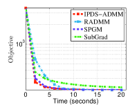
(a) w1a-2477-300

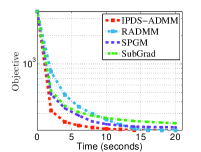
(b) TDT2-500-1000

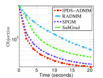
(c) 20News-8000-1000

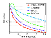
(d) sector-6412-100

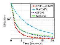
(e) w1a-2477-300

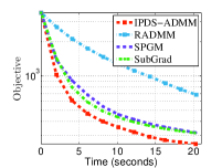
(f) TDT2-500-1000

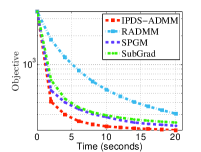
(g) 20News-8000-1000

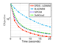
(h) sector-6412-100

Figure 1: The convergence curve of the compared methods for solving sparse PCA with $\rho^{\prime}=10$.

4 Experiments

This section assesses the performance of IPDS-ADMM in solving the sparse PCA problem.

$\blacktriangleright$ Application Model. Sparse PCA enhances traditional PCA by focusing on a subset of informative variables with sparse loadings, thereby reducing model complexity and improving interpretability. It is formulated as follows [9, 31, 23, 19]:

$$\textstyle\min_{{\mathbf{V}}\in\mathbb{R}^{d^{\prime}\times r^{\prime}}}\tfrac{1}{2m^{\prime}}\|{\mathbf{D}}-{\mathbf{D}}{\mathbf{V}}{\mathbf{V}}^{\mathsf{T}}\|_{\mathsf{F}}^{2}+\rho^{\prime}\|{\mathbf{V}}\|_{1},\,s.t.\,{\mathbf{V}}\in\mathcal{M},$$

where $\mathcal{M}\triangleq\{{\mathbf{V}}\,|\,{\mathbf{V}}^{\mathsf{T}}{\mathbf{V}}=\mathbf{I}\}$, ${\mathbf{D}}\in\mathbb{R}^{m^{\prime}\times d^{\prime}}$ is the data matrix. Introducing extra parameter $\mathbf{Y}$, this problem can be formulated as: $\min_{{\mathbf{V}},\mathbf{Y}}\tfrac{1}{2m^{\prime}}\|{\mathbf{D}}-{\mathbf{D}}{\mathbf{V}}{\mathbf{V}}^{\mathsf{T}}\|_{\mathsf{F}}^{2}+\rho^{\prime}\|{\mathbf{V}}\|_{1},\,s.t.\,{\mathbf{V}}=\mathbf{Y},\,\mathbf{Y}\in\mathcal{M}$. It coincides with Problem (1) with ${\mathbf{x}}_{1}={\rm{vec}}(\mathbf{Y})$, ${\mathbf{x}}_{2}={\rm{vec}}({\mathbf{V}})$, $f_{2}({\mathbf{x}}_{2})=\tfrac{1}{2m^{\prime}}\|{\mathbf{D}}-{\mathbf{D}}{\mathbf{V}}{\mathbf{V}}^{\mathsf{T}}\|_{\mathsf{F}}^{2}$, $h_{2}({\mathbf{x}}_{2})=\rho\|{\mathbf{V}}\|_{1}$, $f_{1}({\mathbf{x}}_{1})=0$, $h_{1}({\mathbf{x}}_{1})=\mathcal{I}_{\mathcal{M}}(\mathbf{Y})$, and ${\mathbf{A}}_{1}={\mathbf{A}}_{2}={\mathbf{I}}$ with Condition $\mathbb{BI}$.

$\blacktriangleright$ Compared Methods. We compare IPDS-ADMM against three state-of-the-art general-purpose algorithms that solve Problem (1) (i) the Subgradient method (SubGrad) [25, 10], (ii) the Smoothing Proximal Gradient Method (SPGM) [7], (iii) the Riemannian ADMM with fixed and large penalty (RADMM) [23].

$\blacktriangleright$ Experimental Settings. All methods are implemented in MATLAB on an Intel 2.6 GHz CPU with 64 GB RAM. We incorporate a set of 8 datasets into our experiments, comprising both randomly generated and publicly available real-world data. Appendix Section D describes how to generate the data used in the experiments. For for IPDS-ADMM, we set $(\beta^{0},p,\xi,\delta,\sigma,\theta)=(50\rho^{\prime},1/3,0.9,1/4,1.5,1.01)$ . The penalty parameter for RADMM is set to a reasonably large constant $\beta=500\rho^{\prime}$. We fix $r^{\prime}=20$ and compare objective values for all methods after running $t$ seconds with $t=20$. We provide our code in the supplemental material.

$\blacktriangleright$ Experiment Results. The experimental results depicted in Figure 1 offer the following insights: (i) Sub-Grad tends to be less efficient in comparison to other methods. (ii) SPGM, utilizing a variable smoothing strategy, generally demonstrates slower performance than the multiplier-based variable splitting method. This observation corroborates the widely accepted notion that primal-dual methods are typically more robust and quicker than primal-only methods. (iii) The proposed IPDS-ADMM generally attains the lowest objective function values among all methods examined.

5 Conclusions

In this paper, we introduce IPDS-ADMM, a proximal linearized ADMM that uses an Increasing Penalization and Decreasing Smoothing (IPDS) strategy for solving general multi-block nonconvex composite optimization problems. IPDS-ADMM operates under a relatively relaxed condition, requiring continuity in just one block of the objective function. It incorporates relaxed strategies for dual variable updates when the associated linear operator is either bijective or surjective. We increase the penalty parameter and decrease the smoothing parameter at a controlled pace, and introduce a Lyapunov function for convergence analysis. We also derive the iteration complexity of IPDS-ADMM. Finally, we conduct experiments to demonstrate the effectiveness of our approaches.

Appendix

The organization of the appendix is as follows:

Appendix A covers notations, technical preliminaries, and relevant lemmas.

Appendix B contains proofs related to Section 2.

Appendix C offers proofs related to Section 3.

Appendix D includes additional experiments details and results.

Appendix A Notations, Technical Preliminaries, and Relevant Lemmas

A.1 Notations

We use the following notations in this paper.

• $[n]$: $\{1,2,...,n\}$.

• ${\mathbf{x}}$: ${\mathbf{x}}\triangleq\{{\mathbf{x}}_{1},{\mathbf{x}}_{2},\ldots,{\mathbf{x}}_{n}\}={\mathbf{x}}_{[n]}$.

• ${\mathbf{x}}_{[i,j]}$: ${\mathbf{x}}_{[i,j]}\triangleq\{{\mathbf{x}}_{i},{\mathbf{x}}_{i+1},{\mathbf{x}}_{i+2},\ldots.,{\mathbf{x}}_{j}\}$, where $j\geq i$.

• ${\sf L}_{i}^{t}$: ${\sf L}_{i}^{t}=L_{i}+\beta^{t}\|{\mathbf{A}}_{i}\|_{2}^{2}$. Note that the function $G({\mathbf{x}}^{t},\mathbf{z}^{t};\beta^{t})$ is ${\sf L}_{i}^{t}$-smooth.

• $\sigma_{1}$: $\sigma_{1}\triangleq\tfrac{\sigma}{(1-|1-\sigma|)^{2}}\in\mathbb{R}$, where $\sigma\in(0,2)$. Refer to Lemma A.2.

• $\sigma_{2}$: $\sigma_{2}\triangleq\tfrac{|1-\sigma|}{\sigma(1-|1-\sigma|)}\in\mathbb{R}$, where $\sigma\in(0,2)$. Refer to Lemma A.2.

• $\|\mathbf{x}\|$: Euclidean norm: $\|\mathbf{x}\|=\|\mathbf{x}\|_{2}=\sqrt{\langle\mathbf{x},\mathbf{x}\rangle}$.

• $\langle\mathbf{a},\mathbf{b}\rangle$ : Euclidean inner product, i.e., $\langle\mathbf{a},\mathbf{b}\rangle=\sum_{i}{\mathbf{a}_{i}\mathbf{b}_{i}}$.

• ${\mathbf{A}}^{\mathsf{T}}$ : the transpose of the matrix ${\mathbf{A}}$.

• ${\mathbf{x}}_{i}$: the $i$-th block of the vector ${\mathbf{x}}\in\mathbb{R}^{({\mathbf{d}}_{1}+{\mathbf{d}}_{2}+\ldots+{\mathbf{d}}_{n})\times 1}$ with ${\mathbf{x}}_{i}\in\mathbb{R}^{{\mathbf{d}}_{i}\times 1}$.

• $\overline{\lambda}$: the largest eigenvalue of the matrix $\mathbf{A}_{n}\mathbf{A}_{n}^{\mathsf{T}}$.

• $\underline{\lambda}$: the smallest eigenvalue of the matrix $\mathbf{A}_{n}\mathbf{A}_{n}^{\mathsf{T}}$.

• $\underline{\lambda}^{\prime}$: the smallest eigenvalue of the matrix $\mathbf{A}_{n}^{\mathsf{T}}\mathbf{A}_{n}$.

• $\|{\mathbf{A}}\|$: the spectral norm of the matrix ${\mathbf{A}}$: the largest singular value of ${\mathbf{A}}$.

• ${\mathbf{I}}_{r}$ : ${\mathbf{I}}_{r}\in\mathbb{R}^{r\times r}$, Identity matrix; the subscript is omitted sometimes.

• $\mathcal{I}_{\Xi}(\mathbf{{\mathbf{x}}})$ : the indicator function of a set $\Xi$ with $\mathcal{I}_{\Xi}(\mathbf{{\mathbf{x}}})=0$ if $\mathbf{{\mathbf{x}}}\in\Xi$ and otherwise $+\infty$.

• ${\rm{vec}}(\mathbf{V})$ : ${\rm{vec}}(\mathbf{V})\in\mathbb{R}^{d^{\prime}\times r^{\prime}}$, the vector formed by stacking the column vectors of $\mathbf{V}$.

• ${\rm{mat}}(\mathbf{x})$ : ${\rm{mat}}(\mathbf{x})\in\mathbb{R}^{d^{\prime}\times r^{\prime}}$, Convert $\mathbf{x}\in\mathbb{R}^{(d^{\prime}\cdot r^{\prime})\times 1}$ into a matrix with ${\rm{mat}}({\rm{vec}}(\mathbf{V}))={\mathbf{V}}$.

• $\mathcal{M}$: Orthogonality constraint set: $\mathcal{M}=\{{\mathbf{V}}\,|\,{\mathbf{V}}^{\mathsf{T}}{\mathbf{V}}=\mathbf{I}\}$.

• ${\rm{dist}}^{2}(\Omega,\Omega^{\prime})$ : squared distance between two sets with ${\rm{dist}}^{2}(\Omega,\Omega^{\prime})\triangleq\inf_{\mathbf{w}\in\Omega,\mathbf{w}^{\prime}\in\Omega^{\prime}}\|\mathbf{w}-\mathbf{w}^{\prime}\|_{2}^{2}$.

A.2 Technical Preliminaries

We present some tools in non-smooth analysis including Fréchet subdifferential, limiting (Fréchet) subdifferential, and directional derivative [34, 40, 3]. For any extended real-valued (not necessarily convex) function $F:\mathbb{R}^{n}\rightarrow(-\infty,+\infty]$, its domain is defined by $\text{dom}(F)\triangleq\{{\mathbf{x}}\in\mathbb{R}^{n}:|F({\mathbf{x}})|<+\infty\}$. The Fréchet subdifferential of $F$ at ${\mathbf{x}}\in\text{dom}(F)$, denoted as $\hat{\partial}F({\mathbf{x}})$, is defined as $\hat{\partial}{F}({\mathbf{x}})\triangleq\{\mathbf{v}\in\mathbb{R}^{n}:\lim_{\mathbf{z}\rightarrow{\mathbf{x}}}\inf_{\mathbf{z}\neq{\mathbf{x}}}\tfrac{{F}(\mathbf{z})-{F}({\mathbf{x}})-\langle\mathbf{v},\mathbf{z}-{\mathbf{x}}\rangle}{\|\mathbf{z}-{\mathbf{x}}\|}\geq 0\}$. The limiting subdifferential of ${F}({\mathbf{x}})$ at ${\mathbf{x}}\in\text{dom}({F})$ is defined as: $\partial{F}({\mathbf{x}})\triangleq\{\mathbf{v}\in\mathbb{R}^{n}:\exists{\mathbf{x}}^{k}\rightarrow{\mathbf{x}},{F}({\mathbf{x}}^{k})\rightarrow{F}({\mathbf{x}}),\mathbf{v}^{k}\in\hat{\partial}{F}({\mathbf{x}}^{k})\rightarrow\mathbf{v},\forall k\}$. Note that $\hat{\partial}{F}({\mathbf{x}})\subseteq\partial{F}({\mathbf{x}})$. If $F(\cdot)$ is differentiable at ${\mathbf{x}}$, then $\hat{\partial}{F}({\mathbf{x}})=\partial{F}({\mathbf{x}})=\{\nabla F({\mathbf{x}})\}$ with $\nabla F({\mathbf{x}})$ being the gradient of $F(\cdot)$ at ${\mathbf{x}}$. When $F(\cdot)$ is convex, $\hat{\partial}{F}({\mathbf{x}})$ and $\partial{F}({\mathbf{x}})$ reduce to the classical subdifferential for convex functions, i.e., $\hat{\partial}{F}({\mathbf{x}})=\partial{F}({\mathbf{x}})=\{\mathbf{v}\in\mathbf{R}^{n}:F(\mathbf{z})-F({\mathbf{x}})-\langle\mathbf{v},\mathbf{z}-{\mathbf{x}}\rangle\geq 0,\forall\mathbf{z}\in\mathbb{R}^{n}\}$. The directional derivative of $F(\cdot)$ at ${\mathbf{x}}$ in the direction $\mathbf{v}$ is defined (if it exists) by $F^{\prime}({\mathbf{x}};\mathbf{v})\triangleq\lim_{t\rightarrow 0^{+}}\tfrac{1}{t}(F({\mathbf{x}}+t\mathbf{v})-F({{\mathbf{x}}}))$.

A.3 Relevant Lemmas

We introduce several useful lemmas that will be utilized in this paper.

Lemma A.1.

(Pythagoras Relation) For any vectors $\mathbf{a}\in\mathbb{R}^{n}$, ${\mathbf{b}}\in\mathbb{R}^{n}$, $\mathbf{c}\in\mathbb{R}^{n}$, we have:

$$\tfrac{1}{2}\|\mathbf{a}-{\mathbf{b}}\|_{2}^{2}-\tfrac{1}{2}\|\mathbf{c}-{\mathbf{b}}\|_{2}^{2} = \tfrac{1}{2}\|\mathbf{a}-\mathbf{c}\|_{2}^{2}+\langle{\mathbf{b}}-\mathbf{c},\mathbf{c}-\mathbf{a}\rangle.$$

$$\tfrac{1}{2}\|{\mathbf{b}}\|_{2}^{2}-\tfrac{1}{2}\|\mathbf{c}-{\mathbf{b}}\|_{2}^{2} = \tfrac{1}{2}\|\mathbf{c}\|_{2}^{2}+\langle{\mathbf{b}}-\mathbf{c},\mathbf{c}\rangle.$$

Lemma A.2.

Assume $\sigma\in(0,2)$. Let ${\mathbf{b}}^{+}=\sigma\mathbf{a}+(1-\sigma){\mathbf{b}}$, where ${\mathbf{b}}^{+}\in\mathbb{R}^{n}$, ${\mathbf{b}}\in\mathbb{R}^{n}$, and $\mathbf{a}\in\mathbb{R}^{n}$. We have:

$$\textstyle\tfrac{1}{\sigma}\|{\mathbf{b}}^{+}\|_{2}^{2}\leq\sigma_{1}\|\mathbf{a}\|_{2}^{2}+\sigma_{2}(\|{\mathbf{b}}\|_{2}^{2}-\|{\mathbf{b}}^{+}\|_{2}^{2}),$$

where $\sigma_{1}\triangleq\tfrac{\sigma}{(1-|1-\sigma|)^{2}}$, and $\sigma_{2}\triangleq\tfrac{|1-\sigma|}{\sigma(1-|1-\sigma|)}$.

Proof.

(a) When $\sigma=1$, we have $\sigma_{1}=1$, $\sigma_{2}=0$, and ${\mathbf{b}}^{+}=\mathbf{a}$. The conclusion of this lemma clearly holds.

(b) We now focus on the case when $\sigma\neq 1$. Noticing $|1-\sigma|\neq 0$ and $1-|1-\sigma|\neq 0$, we rewrite ${\mathbf{b}}^{+}=(1-\sigma){\mathbf{b}}+\sigma\mathbf{a}$ into the following equivalent equality

$$\textstyle{\mathbf{b}}^{+}=(1-|1-\sigma|)\cdot\tfrac{\sigma\mathbf{a}}{1-|1-\sigma|}+|1-\sigma|\cdot\tfrac{(1-\sigma){\mathbf{b}}}{|1-\sigma|}.$$

Using the fact that the function $\|\cdot\|_{2}^{2}$ is convex and $|1-\sigma|\in(0,1)$, we derive the following results:

$$\textstyle\|{\mathbf{b}}^{+}\|_{2}^{2} \leq \textstyle(1-|1-\sigma|)\cdot\|\tfrac{\sigma\mathbf{a}}{1-|1-\sigma|}\|_{2}^{2}+|1-\sigma|\cdot\|\tfrac{(1-\sigma){\mathbf{b}}}{|1-\sigma|}\|_{2}^{2}$$

$$\leq \textstyle\tfrac{\sigma^{2}}{1-|1-\sigma|}\cdot\|\mathbf{a}\|_{2}^{2}+|1-\sigma|\cdot\|{\mathbf{b}}\|_{2}^{2}.$$

Subtracting $(|1-\sigma|\cdot\|{\mathbf{b}}^{+}\|_{2}^{2})$ from both sides of the above inequality, we have:

$$\textstyle(1-|1-\sigma|)\|{\mathbf{b}}^{+}\|_{2}^{2}\leq\tfrac{\sigma^{2}}{1-|1-\sigma|}\cdot\|\mathbf{a}\|_{2}^{2}+|1-\sigma|(\|{\mathbf{b}}\|_{2}^{2}-\|{\mathbf{b}}^{+}\|_{2}^{2}).$$

Dividing both sides by $\sigma(1-|1-\sigma|)$, we have:

$$\textstyle\tfrac{1}{\sigma}\|{\mathbf{b}}^{+}\|_{2}^{2}\leq\tfrac{\sigma}{(1-|1-\sigma|)^{2}}\|\mathbf{a}\|_{2}^{2}+\tfrac{|1-\sigma|}{\sigma(1-|1-\sigma|)}(\|{\mathbf{b}}\|_{2}^{2}-\|{\mathbf{b}}^{+}\|_{2}^{2}).$$

Using the definition of $\sigma_{1}$ and $\sigma_{2}$, we finish the proof of this lemma.

∎

Lemma A.3.

We let $t\geq 1$, and $q\in(0,1)$. We have: $\tfrac{1}{q}(t+1)^{q}-\tfrac{1}{q}\geq\tfrac{1}{2}t^{q}$.

Proof.

We let $h(t)\triangleq(t+1)^{q}-1-\tfrac{q}{2}t^{q}$.

Initially, we prove that $f(q)\triangleq 2^{q}-\tfrac{q}{2}-1\geq 0$ for all $q\geq 0$. Given $\nabla f(q)=2^{q}\log(2)-\tfrac{1}{2}\geq 2^{0}\log(2)-\tfrac{1}{2}=0.1931>0$, the function $f(q)$ is increasing for all $q\geq 0$. Combining with the fact that $f(0)=0$, we have: $f(q)\geq 0$ for all $q\geq 0$.

We derive the following inequalities:

$$\nabla h(t)=qt^{q-1}\cdot\{(\tfrac{t+1}{t})^{q-1}-\tfrac{q}{2}\}\overset{\text{\char 172}}{\geq}qt^{p-1}\cdot\{2^{q-1}-\tfrac{q}{2}\}\overset{\text{\char 173}}{\geq}qt^{q-1}\cdot\{\tfrac{q/2+1}{2}-\tfrac{q}{2}\}\overset{\text{\char 174}}{\geq}0,$$

where step ① uses $\tfrac{t+1}{t}\leq 2$ and $q-1\leq 0$; step ② uses $2^{q}\geq\tfrac{q}{2}+1$ for all $q\geq 0$; step ③ uses $1-q\geq 0$. Therefore, $h(t)$ is an increasing function.

Finally, noticing that $h(1)=2^{q}-1-\tfrac{q}{2}\geq 0$, we conclude that $h(t)\geq 0$ for all $t\geq 1$.

∎

Lemma A.4.

We let $p\in(0,1)$. We have: $\tfrac{1}{2}T^{1-p}\leq\sum_{t=1}^{T}t^{-p}\leq\tfrac{T^{(1-p)}}{1-p}$.

Proof.

We define $h(x)=x^{-p}$ and $g(x)=\tfrac{1}{1-p}x^{1-p}$. Clearly, we have: $\nabla g(x)=h(x)$.

By employing the integral test for convergence , we obtain:

$$\textstyle\int_{1}^{T+1}h(x)dx\leq\sum_{t=1}^{T}h(t)\leq h(1)+\int_{1}^{T}h(x)dx.$$ (16)

(a) We have:

$$\textstyle\sum_{t=1}^{T}t^{-p} \overset{\text{\char 172}}{\geq} \textstyle\int_{1}^{T+1}x^{-p}dx$$

$$\overset{\text{\char 173}}{=} \textstyle g(T+1)-g(1)=\tfrac{1}{1-p}(T+1)^{1-p}-\tfrac{1}{1-p}$$

$$\overset{\text{\char 174}}{\geq} \tfrac{1}{2}T^{1-p},$$

where step ① uses the first inequality in (16); step ② uses $\nabla g(x)=h(x)=x^{-p}$; step ③ uses Lemma A.3 with $q=1-p$ and $t=T$.

(b) We have:

$$\textstyle\sum_{t=1}^{T}t^{-p} \overset{\text{\char 172}}{\leq} \textstyle h(1)+\int_{1}^{T}x^{-p}dx$$

$$\overset{\text{\char 173}}{=} \textstyle 1+g(T)-g(1)=1+\tfrac{1}{1-p}(T)^{1-p}-\tfrac{1}{1-p}$$

$$\overset{}{=} \tfrac{T^{(1-p)}-p}{1-p}<\tfrac{T^{(1-p)}}{1-p},$$

where step ① uses the second inequality in (16); step ② uses $h(1)=1$, and $\nabla g(x)=h(x)=x^{-p}$.

∎

Lemma A.5.

We let $p\in(0,1)$ and $t\geq 1$. We have: $(t+1)^{p}-t^{p}\leq pt^{p-1}$.

Proof.

We notice that $h(t)\triangleq t^{p}$ is concave for all $t\geq 1$ and $p\in(0,1)$ since $\nabla h(t)=pt^{p-1}$ and $\nabla^{2}h(t)=p(p-1)t^{p-2}<0$. It follows that: $\forall x,y\geq 1,h(y)-h(x)\leq\langle y-x,\nabla h(x)\rangle$. Letting $x=t$ and $y=t+1$, for all $t\geq 1$ and $p\in(0,1)$, we have: $(t+1)^{p}-t^{p}\leq pt^{p-1}$.

∎

Lemma A.6.

We let $p\in(0,1)$. We have: $\sum_{t=1}^{\infty}(\tfrac{(t+1)^{p}-t^{p}}{t^{p}})^{2}\leq 2$.

Proof.

We have:

$$\textstyle\sum_{t=1}^{\infty}(\tfrac{(t+1)^{p}-t^{p}}{t^{p}})^{2}\overset{\text{\char 172}}{\leq}\textstyle\sum_{t=1}^{\infty}\tfrac{1}{t^{2p}}t^{2p-2}=\sum_{t=1}^{\infty}t^{-2}\overset{\text{\char 173}}{\leq}\textstyle 2,$$

where step ① uses Lemma A.5 and $p\leq 1$; step ② uses $\sum_{t=1}^{\infty}\tfrac{1}{t^{2}}\leq\sum_{t=1}^{\infty}\tfrac{1}{t^{2}}=\tfrac{\pi^{2}}{6}<2$. ∎

Lemma A.7.

Let $\sigma\in(0,2)$, and $e^{t+1}-|1-\sigma|e^{t}\leq\sigma\Psi^{t}$ for all $t\geq 1$. We have: $e^{t}\leq e^{1}+\sigma_{3}\max_{i=1}^{t-1}\Psi^{i}$, where $\sigma_{3}=\tfrac{\sigma}{1-|1-\sigma|}\in[1,\infty)$.

Proof.

Given $\sigma\in(0,2)$, we define $\sigma_{\star}\triangleq|1-\sigma|\in[0,1)$.

We derive the following results:

$$t=1,~{}~{}~{}e^{2} \leq \sigma_{\star}e^{1}+\sigma\Psi^{1}$$

$$t=2,~{}~{}~{}e^{3} \leq \sigma_{\star}e^{2}+\sigma\Psi^{2}\leq\sigma_{\star}^{2}e^{1}+\sigma_{\star}\sigma\Psi^{1}+\sigma\Psi^{2}$$

$$t=3,~{}~{}~{}e^{4} \leq \sigma_{\star}e^{3}+\sigma\Psi^{3}\leq\sigma_{\star}^{3}e^{1}+\sigma_{\star}^{2}\sigma\Psi^{1}+\sigma_{\star}\sigma\Psi^{2}+\sigma\Psi^{3}$$

$$\ldots$$

$$t=T,~{}~{}~{}\textstyle e^{T+1} \leq \textstyle\sigma_{\star}e^{T}+\sigma\Psi^{T}\leq\sigma_{\star}^{T}e^{1}+\sigma\sum_{i=1}^{T}\sigma_{\star}^{T-i}\Psi^{i}.$$

Therefore, we have:

$$\textstyle e^{T+1} \leq \textstyle\sigma_{\star}^{T}e^{1}+\sigma\sum_{i=1}^{T}\sigma_{\star}^{T-i}\Psi^{i}$$

$$\overset{\text{\char 172}}{\leq} \textstyle e^{1}+\sigma\{\max_{i=1}^{T}\Psi^{i}\}\{\sum_{i=1}^{T}\sigma_{\star}^{T-i}\}$$

$$\overset{\text{\char 173}}{\leq} \textstyle e^{1}+\sigma\{\max_{i=1}^{T}\Psi^{i}\}\tfrac{1}{1-\sigma_{\star}},$$

where step ① uses $\sigma_{\star}^{T}\leq 1$; step ② uses the fact that:

$$\textstyle\sum_{i=1}^{T}\sigma_{\star}^{T-i}=\sigma_{\star}^{T-1}+\ldots+\sigma_{\star}^{1}+\sigma_{\star}^{0}=\tfrac{1-\sigma_{\star}^{T}}{1-\sigma_{\star}}\leq\tfrac{1}{1-\sigma_{\star}}.$$

∎

Appendix B Proofs for Section 2

B.1 Proof of Lemma 2.1

Proof.

Consider the update rule $\beta^{t}=\beta^{0}+\beta^{0}\xi t^{p}$, where $p\in(0,1)$.

(a) We have:

$$\textstyle\beta^{t+1}-\beta^{t}-\xi\beta^{t}\overset{\text{\char 172}}{=}\textstyle\beta^{0}\xi((t+1)^{p}-t^{p})-\xi\beta^{0}\overset{\text{\char 173}}{\leq}\beta^{0}\xi-\beta^{0}\xi=0,$$

where step ① uses the update rule $\beta^{t}=\beta^{0}+\beta^{0}\xi t^{p}$; step ② uses the fact that the function $h(t)\triangleq(t+1)^{p}-t^{p}$ is monotonically decreasing w.r.t. $t$ that: $h(t)\leq h(0)=1$.

(b) We derive: $L_{n}\leq\beta^{0}\delta\overline{\lambda}\overset{\text{\char 172}}{\leq}\beta^{t}\delta\overline{\lambda}$, where step ① uses $\beta^{t}\geq\beta^{0}$.

∎

B.2 Proof of Lemma 2.4

Proof.

We let ${\mathbf{u}}$ be a fixed constant vector. We assume $0<\mu_{2}<\mu_{1}$.

We define: $h({\mathbf{u}};\mu)\triangleq\min_{{\mathbf{v}}\in\mathbb{R}^{d\times 1}}h({\mathbf{v}})+\tfrac{1}{2\mu}\|{\mathbf{v}}-{\mathbf{u}}\|_{2}^{2}$.

We define $\mathbb{P}_{h}({\mathbf{u}};\mu)\triangleq\arg\min_{{\mathbf{v}}\in\mathbb{R}^{d\times 1}}h({\mathbf{v}})+\tfrac{1}{2\mu}\|{\mathbf{v}}-{\mathbf{u}}\|_{2}^{2}$.

Initially, by the optimality of $\mathbb{P}_{h}({\mathbf{u}};\mu_{1})$ and $\mathbb{P}_{h}({\mathbf{u}};\mu_{2})$, we obtain:

$${\mathbf{u}}-\mathbb{P}_{h}({\mathbf{u}};\mu_{1})\in\mu_{1}\partial h(\mathbb{P}_{h}({\mathbf{u}};\mu_{1})),$$ (17)

$${\mathbf{u}}-\mathbb{P}_{h}({\mathbf{u}};\mu_{2})\in\mu_{2}\partial h(\mathbb{P}_{h}({\mathbf{u}};\mu_{2})).$$ (18)

For notation simplicity, we define:

$${\mathbf{p}}_{1}\triangleq\mathbb{P}_{h}({\mathbf{u}};\mu_{1}),~{}{\mathbf{g}}_{1}\in\partial h(\mathbb{P}_{h}({\mathbf{u}};\mu_{1}))$$

$${\mathbf{p}}_{2}\triangleq\mathbb{P}_{h}({\mathbf{u}};\mu_{2}),~{}{\mathbf{g}}_{2}\in\partial h(\mathbb{P}_{h}({\mathbf{u}};\mu_{2})).$$

Equations (17) and (18) can be rewritten as:

$${\mathbf{u}}-{\mathbf{p}}_{1}=\mu_{1}{\mathbf{g}}_{1},$$ (19)

$${\mathbf{u}}-{\mathbf{p}}_{2}=\mu_{2}{\mathbf{g}}_{2}.$$ (20)

(a) We now prove that $0\leq\tfrac{h({\mathbf{u}};\mu_{2})-h({\mathbf{u}};\mu_{1})}{\mu_{1}-\mu_{2}}$. We have:

$$h({\mathbf{u}};\mu_{1})-h({\mathbf{u}};\mu_{2}) \overset{\text{\char 172}}{=} \tfrac{1}{2\mu_{1}}\|{\mathbf{u}}-{\mathbf{p}}_{1}\|_{2}^{2}-\tfrac{1}{2\mu_{2}}\|{\mathbf{u}}-{\mathbf{p}}_{2}\|_{2}^{2}+h({\mathbf{p}}_{1})-h({\mathbf{p}}_{2})$$

$$\overset{\text{\char 173}}{\leq} \tfrac{1}{2\mu_{1}}\|{\mathbf{u}}-{\mathbf{p}}_{1}\|_{2}^{2}-\tfrac{1}{2\mu_{2}}\|{\mathbf{u}}-{\mathbf{p}}_{2}\|_{2}^{2}+\langle{\mathbf{p}}_{1}-{\mathbf{p}}_{2},{\mathbf{g}}_{1}\rangle$$

$$\overset{\text{\char 174}}{=} \tfrac{\mu_{1}}{2}\|{\mathbf{g}}_{1}\|_{2}^{2}-\tfrac{\mu_{2}}{2}\|{\mathbf{g}}_{2}\|_{2}^{2}+\langle\mu_{2}{\mathbf{g}}_{2}-\mu_{1}{\mathbf{g}}_{1},{\mathbf{g}}_{1}\rangle$$

$$= -\tfrac{\mu_{1}}{2}\|{\mathbf{g}}_{1}\|_{2}^{2}-\tfrac{\mu_{2}}{2}\|{\mathbf{g}}_{2}\|_{2}^{2}+\mu_{2}\langle{\mathbf{g}}_{2},{\mathbf{g}}_{1}\rangle$$

$$\overset{\text{\char 175}}{\leq} -\tfrac{\mu_{2}}{2}\|{\mathbf{g}}_{1}\|_{2}^{2}-\tfrac{\mu_{2}}{2}\|{\mathbf{g}}_{2}\|_{2}^{2}+\mu_{2}\langle{\mathbf{g}}_{2},{\mathbf{g}}_{1}\rangle$$

$$\overset{}{=} -\tfrac{\mu_{2}}{2}\|{\mathbf{g}}_{2}-{\mathbf{g}}_{1}\|_{2}^{2}\leq 0,$$

where step ① uses the definition of $h({\mathbf{u}};\mu)$; step ② uses the convexity of $h(\cdot)$; step ③ uses the optimality of ${\mathbf{p}}_{1}\triangleq\mathbb{P}_{h}({\mathbf{u}};\mu_{1})$ and ${\mathbf{p}}_{2}\triangleq\mathbb{P}_{h}({\mathbf{u}};\mu_{2})$ as in (19) and (20); step ④ uses $\mu_{2}<\mu_{1}$.

(b) We now prove that $\tfrac{h({\mathbf{u}};\mu_{2})-h({\mathbf{u}};\mu_{1})}{\mu_{1}-\mu_{2}}\leq\tfrac{1}{2}C_{g}^{2}$. We have:

$$h({\mathbf{u}};\mu_{2})-h({\mathbf{u}};\mu_{1}) \overset{\text{\char 172}}{=} \tfrac{1}{2\mu_{2}}\|{\mathbf{u}}-{\mathbf{p}}_{2}\|_{2}^{2}-\tfrac{1}{2\mu_{1}}\|{\mathbf{u}}-{\mathbf{p}}_{1}\|_{2}^{2}+h({\mathbf{p}}_{2})-h({\mathbf{p}}_{1})$$

$$\overset{\text{\char 173}}{\leq} \tfrac{1}{2\mu_{2}}\|{\mathbf{u}}-{\mathbf{p}}_{2}\|_{2}^{2}-\tfrac{1}{2\mu_{1}}\|{\mathbf{u}}-{\mathbf{p}}_{1}\|_{2}^{2}+\langle{\mathbf{p}}_{2}-{\mathbf{p}}_{1},{\mathbf{g}}_{2}\rangle$$

$$\overset{\text{\char 174}}{=} \tfrac{\mu_{2}}{2}\|{\mathbf{g}}_{2}\|_{2}^{2}-\tfrac{\mu_{1}}{2}\|{\mathbf{g}}_{1}\|_{2}^{2}+\langle\mu_{1}{\mathbf{g}}_{1}-\mu_{2}{\mathbf{g}}_{2},{\mathbf{g}}_{2}\rangle$$

$$= -\tfrac{\mu_{2}}{2}\|{\mathbf{g}}_{2}\|_{2}^{2}-\tfrac{\mu_{1}}{2}\|{\mathbf{g}}_{1}\|_{2}^{2}+\mu_{1}\langle{\mathbf{g}}_{2},{\mathbf{g}}_{1}\rangle$$

$$\overset{\text{\char 175}}{\leq} \tfrac{\mu_{1}}{2}\|{\mathbf{g}}_{2}\|_{2}^{2}-\tfrac{\mu_{2}}{2}\|{\mathbf{g}}_{2}\|_{2}^{2}$$

$$\overset{\text{\char 176}}{\leq} \tfrac{\mu_{1}-\mu_{2}}{2}\cdot C_{h}^{2},$$

where step ① uses the definition of $h({\mathbf{u}};\mu)$; step ② uses the convexity of $h(\cdot)$; step ③ uses the optimality of ${\mathbf{p}}_{1}\triangleq\mathbb{P}_{h}({\mathbf{u}};\mu_{1})$ and ${\mathbf{p}}_{2}\triangleq\mathbb{P}_{h}({\mathbf{u}};\mu_{2})$ as in (19) and (20); step ④ uses the inequality that: $-\tfrac{1}{2}\|{\mathbf{g}}_{1}\|_{2}^{2}+\langle{\mathbf{g}}_{1},{\mathbf{g}}_{2}\rangle\leq\tfrac{1}{2}\|{\mathbf{g}}_{2}\|_{2}^{2}$ for all ${\mathbf{g}}_{1}\in\mathbb{R}^{d\times 1}$ and ${\mathbf{g}}_{2}\in\mathbb{R}^{d\times 1}$; step ⑤ uses $\|{\mathbf{g}}_{2}\|\leq C_{h}$. ∎

B.3 Proof of Lemma 2.5

Proof.

We let ${\mathbf{u}}$ be a fixed constant vector. We assume $0<\mu_{2}<\mu_{1}$.

We define: $h({\mathbf{u}};\mu)\triangleq\min_{{\mathbf{v}}\in\mathbb{R}^{d\times 1}}h({\mathbf{v}})+\tfrac{1}{2\mu}\|{\mathbf{v}}-{\mathbf{u}}\|_{2}^{2}$.

We define: $\mathbb{P}_{h}({\mathbf{u}};\mu)\triangleq\arg\min_{{\mathbf{v}}\in\mathbb{R}^{d\times 1}}h({\mathbf{v}})+\tfrac{1}{2\mu}\|{\mathbf{v}}-{\mathbf{u}}\|_{2}^{2}$.

Using Claim (b) of Lemma 2.3, we establish that $h({\mathbf{u}};\mu)$ is smooth w.r.t. ${\mathbf{u}}$, and its gradient can be computed as:

$$\nabla h({\mathbf{u}};\mu)=\mu^{-1}({\mathbf{u}}-\mathbb{P}_{h}({\mathbf{u}};\mu)).$$

We examine the following mapping $\mathcal{H}(\upsilon)\triangleq\upsilon({\mathbf{u}}-\mathbb{P}_{h}({\mathbf{u}};\tfrac{1}{\upsilon}))$ with $\mathcal{H}(\upsilon):\mathbb{R}\mapsto\mathbb{R}^{n}$. We derive:

$$\textstyle\lim_{\delta\rightarrow 0}\tfrac{\mathcal{H}(\upsilon+\delta)-\mathcal{H}(\upsilon)}{\delta} = \textstyle\tfrac{(\upsilon+\delta)({\mathbf{u}}-\mathbb{P}_{h}({\mathbf{u}};\tfrac{1}{\upsilon+\delta}))-\upsilon({\mathbf{u}}-\mathbb{P}_{h}({\mathbf{u}};\tfrac{1}{\upsilon}))}{\delta}$$

$$= \textstyle\tfrac{\delta{\mathbf{u}}-(\upsilon+\delta)\mathbb{P}_{h}({\mathbf{u}};\tfrac{1}{\upsilon})+\upsilon\mathbb{P}_{h}({\mathbf{u}};\tfrac{1}{\upsilon})}{\delta}={\mathbf{u}}-\mathbb{P}_{h}({\mathbf{u}};\tfrac{1}{\upsilon}).$$

Therefore, the first-order derivative of the mapping $\mathcal{H}(\upsilon)$ w.r.t. $\upsilon$ always exists and can be computed as $\nabla_{\upsilon}\mathcal{H}(\upsilon)={\mathbf{u}}-\mathbb{P}_{h}({\mathbf{u}};\tfrac{1}{\upsilon})$, leading to:

$$\forall\upsilon,\upsilon^{\prime}>0,\,\tfrac{\|\mathcal{H}(\upsilon)-\mathcal{H}(\upsilon^{\prime})\|}{|\upsilon-\upsilon^{\prime}|}\leq\|{\mathbf{u}}-\mathbb{P}_{h}({\mathbf{u}};\tfrac{1}{\upsilon})\|.$$

Letting $\upsilon=1/\mu_{1}$ and $\upsilon^{\prime}=1/\mu_{2}$, we derive:

$$\tfrac{\|\nabla h({\mathbf{u}};\mu_{1})-\nabla h({\mathbf{u}};\mu_{2})\|}{|1/\mu_{1}-1/\mu_{2}|}\overset{}{\leq}\|{\mathbf{u}}-\mathbb{P}_{h}({\mathbf{u}};\mu_{1})\|\overset{\text{\char 172}}{=}\mu_{1}\|\partial h(\mathbb{P}_{h}({\mathbf{u}};\mu_{1}))\|\overset{\text{\char 173}}{\leq}\mu_{1}C_{h},$$

where step ① uses the optimality of $\mathbb{P}_{h}({\mathbf{u}};\mu)$ that $\mathbf{0}\in\partial h(\mathbb{P}_{h}({\mathbf{u}};\mu))+\tfrac{1}{\mu}(\mathbb{P}_{h}({\mathbf{u}};\mu)-{\mathbf{u}})$ for all $\mu$; step ② uses the Lipschitz continuity of $h(\cdot)$. We further obtain:

$$\|\nabla\,h({\mathbf{u}};\mu_{1})-\nabla\,h({\mathbf{u}};\mu_{2})\|\leq|1/\mu_{1}-1/\mu_{2}|\mu_{1}C_{h}=(\mu_{1}/\mu_{2}-1)\cdot C_{h}.$$

∎

B.4 Proof of Lemma 2.6

Proof.

The proof of this lemma is similar to that of Lemma 1 in [23]. For completeness, we include the proof here.

We consider the following strongly convex problems:

$${\mathbf{x}}_{n}^{t+1} = \arg\min_{{\mathbf{x}}_{n}}h_{n}({\mathbf{x}}_{n};\mu)+\tfrac{\rho}{2}\|{\mathbf{x}}_{n}-{\mathbf{c}}\|_{2}^{2}$$

$$\Leftrightarrow~{}({\mathbf{x}}_{n}^{t+1},\breve{{\mathbf{x}}}_{n}^{t+1}) = \arg\min_{{\mathbf{x}}_{n},\breve{{\mathbf{x}}}_{n}}h_{n}(\breve{{\mathbf{x}}}_{n})+\tfrac{1}{2\mu}\|{\mathbf{x}}_{n}-\breve{{\mathbf{x}}}_{n}\|_{2}^{2}+\tfrac{\rho}{2}\|{\mathbf{x}}_{n}-{\mathbf{c}}\|_{2}^{2}.$$

We have the following first-order optimality conditions:

$$\mathbf{0} = \tfrac{1}{\mu}({\mathbf{x}}_{n}^{t+1}-\breve{{\mathbf{x}}}_{n}^{t+1})+\rho({\mathbf{x}}_{n}^{t+1}-{\mathbf{c}})$$ (21)

$$\mathbf{0} \in \partial h_{n}(\breve{{\mathbf{x}}}_{n}^{t+1})+\tfrac{1}{\mu}(\breve{{\mathbf{x}}}_{n}^{t+1}-{\mathbf{x}}_{n}^{t+1}).$$ (22)

(a) Using (21), we obtain: ${\mathbf{x}}_{n}^{t+1}=\tfrac{1}{1/\mu+\rho}(\tfrac{1}{\mu}\breve{{\mathbf{x}}}_{n}^{t+1}+\rho{\mathbf{c}})$. Plugging this equation into (22) yields:

$$\mathbf{0} \in \partial h_{n}(\breve{{\mathbf{x}}}_{n}^{t+1})+\tfrac{1}{\mu}(\breve{{\mathbf{x}}}_{n}^{t+1}-\tfrac{1}{1/\mu+\rho}(\tfrac{1}{\mu}\breve{{\mathbf{x}}}_{n}^{t+1}+\rho{\mathbf{c}}))$$

$$= \partial h_{n}(\breve{{\mathbf{x}}}_{n}^{t+1})+\tfrac{\rho}{1+\mu\rho}(\breve{{\mathbf{x}}}_{n}^{t+1}-{\mathbf{c}}).$$

The inclusion above implies that:

$$\breve{{\mathbf{x}}}_{n}^{t+1}=\arg\min_{\breve{{\mathbf{x}}}_{n}}h_{n}(\breve{{\mathbf{x}}}_{n})+\tfrac{1}{2}\cdot\tfrac{\rho}{1+\mu\rho}\|\breve{{\mathbf{x}}}_{n}-{\mathbf{c}}\|_{\mathsf{F}}^{2}.$$

(b) We derive:

$$-\rho({\mathbf{x}}_{n}^{t+1}-{\mathbf{c}})\overset{\text{\char 172}}{=}\tfrac{1}{\mu}({\mathbf{x}}_{n}^{t+1}-\breve{{\mathbf{x}}}_{n}^{t+1})\overset{\text{\char 173}}{\in}\partial h_{n}(\breve{{\mathbf{x}}}_{n}^{t+1}),$$

where step ① uses (21); step ② uses (22).

(c) Using (22), we have: $\breve{{\mathbf{x}}}_{n}^{t+1}-{\mathbf{x}}_{n}^{t+1}=-\mu\partial h_{n}(\breve{{\mathbf{x}}}_{n}^{t+1})$. This leads to $\|\breve{{\mathbf{x}}}_{n}^{t+1}-{\mathbf{x}}_{n}^{t+1}\|\leq\mu C_{h}$.

∎

Appendix C Proofs for Section 3

C.1 Proof of Lemma 3.1

Proof.

(a) We now focus on sufficient decrease for variables $\{{\mathbf{x}}_{1},{\mathbf{x}}_{2},\ldots,{\mathbf{x}}_{n-1}\}$. We define $\Phi_{i}^{t}=G({\mathbf{x}}^{t+1}_{[1,i-1]},{\mathbf{x}}^{t+1}_{i},{\mathbf{x}}^{t}_{[i+1,n]},\mathbf{z}^{t};\beta^{t})-G({\mathbf{x}}^{t+1}_{[1,i-1]},{\mathbf{x}}^{t}_{i},{\mathbf{x}}^{t}_{[i+1,n]},\mathbf{z}^{t};\beta^{t})+h_{i}({\mathbf{x}}_{i}^{t+1})-h_{i}({\mathbf{x}}_{i}^{t})$, where $i\in[n-1]$.

Noticing the function $G({\mathbf{x}}^{t+1}_{[1,i-1]},{\mathbf{x}}_{i},{\mathbf{x}}^{t}_{[i+1,n]},\mathbf{z}^{t};\beta^{t})$ is ${\sf L}_{i}^{t}$-smooth w.r.t. ${\mathbf{x}}_{i}$ for the $t$-th iteration, we have:

$$G({\mathbf{x}}^{t+1}_{[1,i-1]},{\mathbf{x}}^{t+1}_{i},{\mathbf{x}}^{t}_{[i+1,n]},\mathbf{z}^{t};\beta^{t})-G({\mathbf{x}}^{t+1}_{[1,i-1]},{\mathbf{x}}^{t}_{i},{\mathbf{x}}^{t}_{[i+1,n]},\mathbf{z}^{t};\beta^{t})$$ (23)

$$\leq \langle{\mathbf{x}}_{i}^{t+1}-{\mathbf{x}}_{i}^{t},\nabla_{{\mathbf{x}}_{i}}G({\mathbf{x}}^{t+1}_{[1,n-1]},{\mathbf{x}}_{i}^{t},{\mathbf{x}}_{[i+1,n]}^{t},\mathbf{z}^{t};\beta^{t})\rangle+\tfrac{{\sf L}_{i}^{t}}{2}\|{\mathbf{x}}_{i}^{t+1}-{\mathbf{x}}_{i}^{t}\|_{2}^{2}.$$

Given ${\mathbf{x}}_{i}^{t+1}$ is the minimizer of the following optimization problem:

$$\textstyle{\mathbf{x}}_{i}^{t+1}\in\arg\min_{{\mathbf{x}}_{i}}\,h_{i}({\mathbf{x}}_{i})+\langle{\mathbf{x}}_{i}-{\mathbf{x}}_{i}^{t},\nabla_{{\mathbf{x}}_{i}}G({\mathbf{x}}^{t+1}_{[1,n-1]},{\mathbf{x}}_{i}^{t},{\mathbf{x}}_{[i+1,n]}^{t},\mathbf{z}^{t};\beta^{t})\rangle+\tfrac{\theta_{1}{\sf L}_{i}^{t}}{2}\|{\mathbf{x}}_{i}-{\mathbf{x}}_{i}^{t}\|_{2}^{2}.$$

The optimality of ${\mathbf{x}}_{i}^{t+1}$ leads to:

$$\textstyle h_{i}({\mathbf{x}}_{i}^{t+1})-h_{i}({\mathbf{x}}_{i}^{t})+\langle{\mathbf{x}}_{i}^{t+1}-{\mathbf{x}}_{i}^{t},\nabla_{{\mathbf{x}}_{i}}G({\mathbf{x}}^{t+1}_{[1,n-1]},{\mathbf{x}}_{i}^{t},{\mathbf{x}}_{[i+1,n]}^{t},\mathbf{z}^{t};\beta^{t})\rangle\overset{\text{}}{\leq}\textstyle-\tfrac{\theta_{1}{\sf L}_{i}^{t}}{2}\|{\mathbf{x}}_{i}^{t+1}-{\mathbf{x}}_{i}^{t}\|_{2}^{2}.$$ (24)

Combining equations (23) and (24), we derive the following expressions:

$$\Phi_{i}^{t}\leq(\tfrac{1}{2}-\tfrac{\theta_{1}}{2})\cdot{\sf L}_{i}^{t}\|{\mathbf{x}}_{i}^{t+1}-{\mathbf{x}}_{i}^{t}\|_{2}^{2}.$$

Telescoping the above inequality over $i$ from $1$ to $(n-1)$ leads to:

$$\textstyle\sum_{i=1}^{n-1}\Phi_{i}^{t}\leq\sum_{i=1}^{n-1}\{(\tfrac{1}{2}-\tfrac{\theta_{1}}{2})\cdot{\sf L}_{i}^{t}\|{\mathbf{x}}_{i}^{t+1}-{\mathbf{x}}_{i}^{t}\|_{2}^{2}\}.$$

Therefore, we obtain:

$$\textstyle\mathcal{L}({\mathbf{x}}_{[1,n-1]}^{t+1},{\mathbf{x}}_{n}^{t},\mathbf{z}^{t};\beta^{t},\mu^{t})-\mathcal{L}({\mathbf{x}}^{t},\mathbf{z}^{t};\beta^{t},\mu^{t})\leq\sum_{i=1}^{n-1}\{(\tfrac{1}{2}-\tfrac{\theta_{1}}{2})\cdot{\sf L}_{i}^{t}\|{\mathbf{x}}_{i}^{t+1}-{\mathbf{x}}_{i}^{t}\|_{2}^{2}\}.$$ (25)

(b) We now focus on sufficient decrease for variable $\{{\mathbf{x}}_{n}\}$. Noticing the function $G({\mathbf{x}}^{t+1}_{[1,n-1]},{\mathbf{x}}_{n},\mathbf{z}^{t};\beta^{t})$ is ${\sf L}_{n}^{t}$-smooth w.r.t. ${\mathbf{x}}_{n}$ for the $t$-th iteration, we have:

$$G({\mathbf{x}}^{t+1}_{[1,n-1]},{\mathbf{x}}^{t+1}_{n},\mathbf{z}^{t};\beta^{t})-G({\mathbf{x}}^{t+1}_{[1,n-1]},{\mathbf{x}}^{t}_{n},\mathbf{z}^{t};\beta^{t})$$ (26)

$$\leq \langle{\mathbf{x}}_{n}^{t+1}-{\mathbf{x}}_{n}^{t},\nabla_{{\mathbf{x}}_{n}}G({\mathbf{x}}^{t+1}_{[1,n-1]},{\mathbf{x}}_{n}^{t},\mathbf{z}^{t};\beta^{t})\rangle+\tfrac{{\sf L}_{n}^{t}}{2}\|{\mathbf{x}}_{n}^{t+1}-{\mathbf{x}}_{n}^{t}\|_{2}^{2}.$$

Since $h_{n}({\mathbf{x}}_{n};\mu^{t})$ is convex, we have:

$$h_{n}({\mathbf{x}}_{n}^{t+1};\mu^{t})-h_{n}({\mathbf{x}}_{n}^{t};\mu^{t})$$ (27)

$$\leq \langle{\mathbf{x}}_{n}^{t+1}-{\mathbf{x}}_{n}^{t+1},\nabla h_{n}({\mathbf{x}}_{i}^{t+1};\mu^{t})\rangle$$

$$\overset{\text{\char 172}}{=} \langle{\mathbf{x}}_{n}^{t+1}-{\mathbf{x}}_{n}^{t+1},-\nabla_{{\mathbf{x}}_{n}}G({\mathbf{x}}^{t+1}_{[1,n-1]},{\mathbf{x}}_{n}^{t},\mathbf{z}^{t};\beta^{t})\rangle-\theta_{2}{\sf L}_{n}^{t}({\mathbf{x}}_{n}^{t+1}-{\mathbf{x}}_{n}^{t})\rangle,$$

where step ① uses the the first-order optimality condition of ${\mathbf{x}}_{n}^{t+1}$ that:

$$\textstyle\mathbf{0}=\nabla h_{n}({\mathbf{x}}_{n}^{t+1};\mu^{t})+\nabla_{{\mathbf{x}}_{n}}G({\mathbf{x}}^{t+1}_{[1,n-1]},{\mathbf{x}}_{n}^{t},\mathbf{z}^{t};\beta^{t})\rangle+\theta_{2}{\sf L}_{n}^{t}({\mathbf{x}}_{n}^{t+1}-{\mathbf{x}}_{n}^{t}).$$

Adding Inequalities (26) and (27) together, we have:

$$h_{n}({\mathbf{x}}_{n}^{t+1};\mu^{t})-h_{n}({\mathbf{x}}_{n}^{t};\mu^{t})+G({\mathbf{x}}^{t+1}_{[1,n-1]},{\mathbf{x}}^{t+1}_{n},\mathbf{z}^{t};\beta^{t})-G({\mathbf{x}}^{t+1}_{[1,n-1]},{\mathbf{x}}^{t}_{n},\mathbf{z}^{t};\beta^{t})$$

$$\leq \tfrac{{\sf L}_{n}^{t}}{2}\|{\mathbf{x}}_{n}^{t+1}-{\mathbf{x}}_{n}^{t}\|_{2}^{2}-\theta_{2}{\sf L}_{n}^{t}\|{\mathbf{x}}_{n}^{t+1}-{\mathbf{x}}_{n}^{t}\|_{2}^{2}$$

$$= (\tfrac{1}{2}-\theta_{2})\cdot{\sf L}_{n}^{t}\|{\mathbf{x}}_{n}^{t+1}-{\mathbf{x}}_{n}^{t}\|_{2}^{2}.$$

This results in the following inequality:

$$\mathcal{L}({\mathbf{x}}^{t+1},\mathbf{z}^{t};\beta^{t},\mu^{t})-\mathcal{L}({\mathbf{x}}_{[1,n-1]}^{t+1},{\mathbf{x}}_{n}^{t},\mathbf{z}^{t};\beta^{t},\mu^{t})\leq(\tfrac{1}{2}-\theta_{2})\cdot{\sf L}_{n}^{t}\|{\mathbf{x}}_{n}^{t+1}-{\mathbf{x}}_{n}^{t}\|_{2}^{2}.$$ (28)

(c) We now focus on sufficient decrease for variable $\{{\mathbf{z}}\}$. We have:

$$\mathcal{L}({\mathbf{x}}^{t+1},\mathbf{z}^{t+1};\beta^{t},\mu^{t})-\mathcal{L}({\mathbf{x}}^{t+1},\mathbf{z}^{t};\beta^{t},\mu^{t})$$ (29)

$$= \langle{\mathbf{A}}{\mathbf{x}}^{t+1}-{\mathbf{b}},{\mathbf{z}}^{t+1}-{\mathbf{z}}^{t}\rangle$$

$$\overset{\text{\char 172}}{=} \langle\tfrac{1}{\sigma\beta^{t}}({\mathbf{z}}^{t+1}-{\mathbf{z}}^{t}),{\mathbf{z}}^{t+1}-{\mathbf{z}}^{t}\rangle$$

$$= \tfrac{1}{\sigma\beta^{t}}\|{\mathbf{z}}^{t+1}-{\mathbf{z}}^{t}\|_{2}^{2},$$

where step ① uses ${\mathbf{z}}^{t+1}={\mathbf{z}}^{t}+\sigma\beta^{t}({\mathbf{A}}{\mathbf{x}}^{t+1}-{\mathbf{b}})$ with ${\mathbf{A}}{\mathbf{x}}^{t+1}\triangleq\sum_{j=1}^{n}{\mathbf{A}}_{j}{\mathbf{x}}_{j}^{t+1}$.

(d) We now focus on sufficient decrease for variable $\{\beta\}$. We have:

$$\textstyle\mathcal{L}({\mathbf{x}}^{t+1},\mathbf{z}^{t+1};\beta^{t+1},\mu^{t})-\mathcal{L}({\mathbf{x}}^{t+1},\mathbf{z}^{t+1};\beta^{t},\mu^{t})$$ (30)

$$= \textstyle(\tfrac{\beta^{t+1}}{2}-\tfrac{\beta^{t}}{2})\|{\mathbf{A}}{\mathbf{x}}^{t+1}-{\mathbf{b}}\|_{2}^{2}$$

$$\overset{\text{\char 172}}{=} (\tfrac{\beta^{t+1}}{2}-\tfrac{\beta^{t}}{2})\|\tfrac{1}{\sigma\beta^{t}}({\mathbf{z}}^{t+1}-{\mathbf{z}}^{t})\|_{2}^{2}$$

$$\overset{\text{\char 173}}{\leq} \textstyle(\tfrac{(1+\xi)\beta^{t}}{2}-\tfrac{\beta^{t}}{2})\|\tfrac{1}{\sigma\beta^{t}}({\mathbf{z}}^{t+1}-{\mathbf{z}}^{t})\|_{2}^{2}$$

$$= \textstyle\tfrac{\xi}{2\sigma}\cdot\tfrac{1}{\sigma\beta^{t}}\|{\mathbf{z}}^{t+1}-{\mathbf{z}}^{t}\|_{2}^{2},$$

where step ① uses ${\mathbf{z}}^{t+1}={\mathbf{z}}^{t}+\sigma\beta^{t}({\mathbf{A}}{\mathbf{x}}^{t+1}-{\mathbf{b}})$; step ② uses Lemma 2.1 that $\beta^{t+1}\leq\beta^{t}(1+\xi)$.

(e) We now focus on sufficient decrease for variable $\{\mu\}$. We have:

$$\mathcal{L}({\mathbf{x}}^{t+1},\mathbf{z}^{t+1};\beta^{t+1},\mu^{t+1})-\mathcal{L}({\mathbf{x}}^{t+1},\mathbf{z}^{t+1};\beta^{t+1},\mu^{t})$$ (31)

$$= h_{n}({\mathbf{x}}^{t+1}_{n};\mu^{t+1})-h_{n}({\mathbf{x}}^{t+1}_{n};\mu^{t})$$

$$\overset{\text{\char 172}}{\leq} \tfrac{1}{2}C_{h}(\mu^{t}-\mu^{t+1}),$$

where step ① uses Lemma 2.4.

Combining Inequalities (25), (28), (29), (30), and (31), we have:

$$\mathcal{L}({\mathbf{x}}^{t+1},\mathbf{z}^{t+1};\beta^{t+1},\mu^{t+1})-\mathcal{L}({\mathbf{x}}^{t},\mathbf{z}^{t};\beta^{t},\mu^{t})$$ (32)

$$\leq \textstyle[\sum_{i=1}^{n-1}\{(\tfrac{1}{2}-\tfrac{\theta_{1}}{2})\cdot{\sf L}_{i}^{t}\|{\mathbf{x}}_{i}^{t+1}-{\mathbf{x}}_{i}^{t}\|_{2}^{2}\}]+(\tfrac{1}{2}-\theta_{2})\cdot{\sf L}_{n}^{t}\|{\mathbf{x}}_{n}^{t+1}-{\mathbf{x}}_{n}^{t}\|_{2}^{2}$$

$$(1+\tfrac{\xi}{2\sigma})\cdot\tfrac{1}{\sigma\beta^{t}}\|{\mathbf{z}}^{t+1}-{\mathbf{z}}^{t}\|_{2}^{2}+\tfrac{1}{2}C_{h}(\mu^{t}-\mu^{t+1})$$

We define $\Theta^{t}_{L}\triangleq\mathcal{L}({\mathbf{x}}^{t},\mathbf{z}^{t};\beta^{t},\mu^{t})+\tfrac{1}{2}C_{h}\mu^{t}$, $\varepsilon_{3}\triangleq\xi$, $\varepsilon_{1}\triangleq\tfrac{1}{2}\theta_{1}-\tfrac{1}{2}$, and $\mathcal{E}^{t+1}\triangleq\textstyle\tfrac{\varepsilon_{3}}{\beta^{t}}\|{\mathbf{z}}^{t+1}-{\mathbf{z}}^{t}\|_{2}^{2}+\varepsilon_{2}{\sf L}_{n}^{t}\|{\mathbf{x}}_{n}^{t+1}-{\mathbf{x}}_{n}^{t}\|_{2}^{2}+\varepsilon_{1}\sum_{i=1}^{n-1}{\sf L}_{i}^{t}\|{\mathbf{x}}_{i}^{t+1}-{\mathbf{x}}_{i}^{t}\|_{2}^{2}$. We have:

$$\mathcal{E}^{t+1}+\Theta^{t+1}_{L}-\Theta^{t}_{L}$$

$$\leq \textstyle(\tfrac{1}{2}-\theta_{2}+\varepsilon_{2})\cdot{\sf L}_{n}^{t}\|{\mathbf{x}}_{n}^{t+1}-{\mathbf{x}}_{n}^{t}\|_{2}^{2}+(1+\tfrac{\xi}{2\sigma}+\sigma\xi)\cdot\tfrac{1}{\sigma\beta^{t}}\|{\mathbf{z}}^{t+1}-{\mathbf{z}}^{t}\|_{2}^{2}.$$

∎

C.2 Proof of Lemma 3.2

Proof.

For any $i\in[n]$, we define ${\mathbbm{u}}_{i}^{t+1}\triangleq\bm{\theta}_{i}{\sf L}_{i}^{t}[{\mathbf{x}}_{i}^{t+1}-{\mathbf{x}}_{i}^{t}]-\beta^{t}{\mathbf{A}}_{i}^{\mathsf{T}}[\sum_{j=i}^{n}{\mathbf{A}}_{j}({\mathbf{x}}_{j}^{t+1}-{\mathbf{x}}_{j}^{t})]$, and let $\mathbbm{w}_{i}^{t+1}\in\partial h_{i}({\mathbf{x}}_{i}^{t+1})+\nabla f_{i}({\mathbf{x}}_{i}^{t})$.

We notice that ${\mathbf{x}}_{i}^{t+1}$ is the minimizer of the following problem:

$$\textstyle{\mathbf{x}}_{i}^{t+1}\in\arg\min_{{\mathbf{x}}_{i}}\,\tfrac{\theta{\sf L}_{i}^{t}}{2}\|{\mathbf{x}}_{i}-{\mathbf{x}}_{i}^{t}\|_{2}^{2}+h_{i}({\mathbf{x}}_{i})+\langle{\mathbf{x}}_{i}-{\mathbf{x}}_{i}^{t},\nabla_{{\mathbf{x}}_{i}}G({\mathbf{x}}_{[1,i-1]}^{t+1},{\mathbf{x}}_{[i,n]}^{t},\mathbf{z}^{t};\beta^{t})\rangle.$$

Using the necessary first-order optimality condition of the solution ${\mathbf{x}}_{i}^{t+1}$, we have:

$$\nabla_{{\mathbf{x}}_{i}}G({\mathbf{x}}_{[1,i-1]}^{t+1},{\mathbf{x}}_{[i,n]}^{t},\mathbf{z}^{t};\beta^{t})\in-\partial h_{i}({\mathbf{x}}_{i}^{t+1})-\theta{\sf L}_{i}^{t}({\mathbf{x}}_{i}^{t+1}-{\mathbf{x}}_{i}^{t}).$$ (33)

Using the definition of the function $G({\mathbf{x}},\mathbf{z};\beta)\triangleq\langle[\sum_{j=1}^{n}{\mathbf{A}}_{j}{\mathbf{x}}_{j}]-{\mathbf{b}},\mathbf{z}\rangle+\tfrac{\beta}{2}\|[\sum_{j=1}^{n}{\mathbf{A}}_{j}{\mathbf{x}}_{j}]-{\mathbf{b}}\|_{2}^{2}+\sum_{j=1}^{n}f_{j}({\mathbf{x}}_{j})$, we have:

$$\nabla_{{\mathbf{x}}_{i}}G({\mathbf{x}}_{[1,i-1]}^{t+1},{\mathbf{x}}_{[i,n]}^{t},\mathbf{z}^{t};\beta^{t})$$ (34)

$$= \textstyle\nabla f_{i}({\mathbf{x}}_{i}^{t})+{\mathbf{A}}_{i}^{\mathsf{T}}\mathbf{z}^{t}+\beta^{t}{\mathbf{A}}_{i}^{\mathsf{T}}\{[\sum_{j=1}^{i-1}{\mathbf{A}}_{j}{\mathbf{x}}_{j}^{t+1}]+[\sum_{j=i}^{n}{\mathbf{A}}_{j}{\mathbf{x}}_{j}^{t}]-{\mathbf{b}}\}$$

$$= \textstyle\nabla f_{i}({\mathbf{x}}_{i}^{t})+{\mathbf{A}}_{i}^{\mathsf{T}}\mathbf{z}^{t}+\beta^{t}{\mathbf{A}}_{i}^{\mathsf{T}}\{{\mathbf{A}}{\mathbf{x}}^{t+1}-{\mathbf{b}}+[\sum_{j=i}^{n}{\mathbf{A}}_{j}({\mathbf{x}}_{j}^{t}-{\mathbf{x}}_{j}^{t+1})]\}$$

$$\overset{\text{\char 172}}{=} \textstyle\nabla f_{i}({\mathbf{x}}_{i}^{t})+{\mathbf{A}}_{i}^{\mathsf{T}}\mathbf{z}^{t}+\tfrac{1}{\sigma}{\mathbf{A}}_{i}^{\mathsf{T}}(\mathbf{z}^{t+1}-\mathbf{z}^{t})+\beta^{t}{\mathbf{A}}_{i}^{\mathsf{T}}\{\sum_{j=i}^{n}{\mathbf{A}}_{j}({\mathbf{x}}_{j}^{t}-{\mathbf{x}}_{j}^{t+1})\},$$

where step ① uses the update rule of $\mathbf{z}^{t+1}$ that $\mathbf{z}^{t+1}-\mathbf{z}^{t}=\sigma\beta^{t}(\sum_{i=1}^{n}{\mathbf{A}}_{i}{\mathbf{x}}_{i}^{t+1}-{\mathbf{b}})$. Combining the Equalities (33) and (34), we obtain the following result:

$$\textstyle\mathbf{0} \in \partial h_{i}({\mathbf{x}}_{i}^{t+1})+\bm{\theta}_{i}{\sf L}_{i}^{t}[{\mathbf{x}}_{i}^{t+1}-{\mathbf{x}}_{i}^{t}]+\nabla f_{i}({\mathbf{x}}_{i}^{t})$$

$$\textstyle+{\mathbf{A}}_{i}^{\mathsf{T}}\mathbf{z}^{t}+\beta^{t}{\mathbf{A}}_{i}^{\mathsf{T}}[\sum_{j=i}^{n}{\mathbf{A}}_{j}({\mathbf{x}}_{j}^{t}-{\mathbf{x}}_{j}^{t+1})]+\tfrac{1}{\sigma}{\mathbf{A}}_{i}^{\mathsf{T}}(\mathbf{z}^{t+1}-\mathbf{z}^{t})$$

Using the definition of $\mathbbm{w}_{i}^{t+1}$ and ${\mathbbm{u}}_{i}^{t+1}$ for all $i\in[n]$, we have: $\mathbf{0}=\mathbbm{w}_{i}^{t+1}+{\mathbbm{u}}_{i}^{t+1}+{\mathbf{A}}_{i}^{\mathsf{T}}\mathbf{z}^{t}+\tfrac{1}{\sigma}{\mathbf{A}}_{i}^{\mathsf{T}}(\mathbf{z}^{t+1}-\mathbf{z}^{t})$. Multiplying both sides by $\sigma\in(0,2)$, for all $t\geq 0$, we have:

$$\textstyle\mathbf{0}=\sigma\mathbbm{w}_{i}^{t+1}+\sigma{\mathbf{A}}_{i}^{\mathsf{T}}\mathbf{z}^{t}+{\mathbf{A}}_{i}^{\mathsf{T}}(\mathbf{z}^{t+1}-\mathbf{z}^{t})+\sigma{\mathbbm{u}}_{i}^{t+1}.$$ (35)

Given that $t$ can take on any integer value, for all $t\geq 1$, we derive:

$$\textstyle\mathbf{0}=\sigma\mathbbm{w}_{i}^{t}+\sigma{\mathbf{A}}_{i}^{\mathsf{T}}\mathbf{z}^{t-1}+{\mathbf{A}}_{i}^{\mathsf{T}}(\mathbf{z}^{t}-\mathbf{z}^{t-1})+\sigma{\mathbbm{u}}_{i}^{t}.$$ (36)

Combining Equality (35) and Equality (36), for all $t\geq 1$, we have:

$${\mathbf{A}}_{i}^{\mathsf{T}}(\mathbf{z}^{t+1}-\mathbf{z}^{t})=(1-\sigma){\mathbf{A}}_{i}^{\mathsf{T}}(\mathbf{z}^{t}-\mathbf{z}^{t-1})-\sigma(\mathbbm{w}_{i}^{t+1}-\mathbbm{w}_{i}^{t})-\sigma({\mathbbm{u}}_{i}^{t+1}-{\mathbbm{u}}_{i}^{t})$$ (37)

In view of (37), we let $i=n$ and arrive at the following three distinct identities:

$$\mathbb{BI}: \underbrace{{\mathbf{A}}_{n}^{\mathsf{T}}(\mathbf{z}^{t+1}-\mathbf{z}^{t})}_{\triangleq\mathbbm{a}^{t+1}}=(1-\sigma)\underbrace{({\mathbf{A}}_{n}^{\mathsf{T}}(\mathbf{z}^{t}-\mathbf{z}^{t-1}))}_{\triangleq\mathbbm{a}^{t}}+\sigma\underbrace{({\mathbbm{u}}_{n}^{t}-{\mathbbm{u}}_{n}^{t+1}+\mathbbm{w}_{n}^{t}-\mathbbm{w}_{n}^{t+1})}_{\mathbbm{c}^{t}}.$$

$$\mathbb{SU}: \underbrace{{\mathbf{A}}_{n}^{\mathsf{T}}(\mathbf{z}^{t+1}-\mathbf{z}^{t})+\sigma{\mathbbm{u}}_{n}^{t+1}}_{\triangleq\mathbbm{a}^{t+1}}=(1-\sigma)(\underbrace{{\mathbf{A}}_{n}^{\mathsf{T}}(\mathbf{z}^{t}-\mathbf{z}^{t-1})+\sigma{\mathbbm{u}}_{n}^{t}}_{\triangleq\mathbbm{a}^{t}})+\sigma(\underbrace{\sigma{\mathbbm{u}}_{n}^{t}+\mathbbm{w}_{n}^{t}-\mathbbm{w}_{n}^{t+1}}_{\triangleq\mathbbm{c}^{t}}).$$

$${\mathbf{A}}_{n}^{\mathsf{T}}(\mathbf{z}^{t+1}-\mathbf{z}^{t})+\sigma\mathbbm{w}_{n}^{t+1}=(1-\sigma)({\mathbf{A}}_{n}^{\mathsf{T}}(\mathbf{z}^{t}-\mathbf{z}^{t-1})+\sigma\mathbbm{w}_{n}^{t})+\sigma(\sigma\mathbbm{w}_{n}^{t}+{\mathbbm{u}}_{n}^{t}-{\mathbbm{u}}_{n}^{t+1}).$$

Notably, our attention is specifically directed towards the first two formulations.

∎

C.3 Proof of Lemma 3.3

Proof.

We denote ${\mathbf{Q}}^{t}\triangleq\theta_{2}{\sf L}_{n}^{t}\mathbf{I}-\beta^{t}{\mathbf{A}}_{n}^{\mathsf{T}}{\mathbf{A}}_{n}\in\mathbb{R}^{\mathbf{d}_{i}\times\mathbf{d}_{i}}$.

We assume ${\mathbf{A}}_{n}^{\mathsf{T}}{\mathbf{A}}_{n}$ has the singular value decomposition ${\mathbf{A}}_{n}^{\mathsf{T}}{\mathbf{A}}_{n}=\tilde{\mathbf{U}}^{\mathsf{T}}{\rm{diag}}(\bm{\lambda})\tilde{\mathbf{U}}$, where $\tilde{\mathbf{U}}\in\mathbb{R}^{\mathbf{d}_{i}\times\mathbf{d}_{i}}$, $\bm{\lambda}\in\mathbb{R}^{\mathbf{d}_{i}\times 1}$, and $\tilde{\mathbf{U}}^{\mathsf{T}}\tilde{\mathbf{U}}=\tilde{\mathbf{U}}\tilde{\mathbf{U}}^{\mathsf{T}}=\mathbf{I}_{\mathbf{d}_{i}}$. Here, ${\rm{diag}}(\bm{\lambda})$ denotes a diagonal matrix with $\bm{\lambda}$ as the main diagonal entries.

(a) We derive:

$$\textstyle{\sf L}_{n}^{t}\triangleq L_{n}+\beta^{t}\overline{\lambda}\overset{\text{\char 172}}{\leq}\beta^{t}\overline{\lambda}(\delta+1),$$ (38)

where step ① uses Lemma 2.1 that $L_{n}\leq\delta\beta^{t}\overline{\lambda}$.

(b) We have:

$$\|{\mathbf{Q}}^{t}\|\overset{\text{\char 172}}{=}\|\theta_{2}{\sf L}_{n}^{t}-\beta^{t}\bm{\lambda}\|_{\infty}\overset{\text{\char 173}}{=}\theta_{2}{\sf L}_{n}^{t}-\min(\beta^{t}\bm{\lambda})\overset{\text{\char 174}}{\leq}\overline{\lambda}\beta^{t}\cdot(\underbrace{{\theta_{2}(1+\delta)}-\underline{\lambda}^{\prime}/\overline{\lambda}}_{\triangleq q}),$$

where step ① uses $\|\theta_{2}{\sf L}_{n}^{t}\mathbf{I}-\beta^{t}{\mathbf{A}}_{n}^{\mathsf{T}}{\mathbf{A}}_{n}\|=\|\tilde{\mathbf{U}}^{\mathsf{T}}{\rm{diag}}(\theta_{2}{\sf L}_{n}^{t}-\beta^{t}\bm{\lambda})\tilde{\mathbf{U}}\|=\|\theta_{2}{\sf L}_{n}^{t}-\beta^{t}\bm{\lambda}\|_{\infty}$; step ② uses the fact that $\|\rho-{\mathbf{x}}\|_{\infty}=\max(\rho-{\mathbf{x}})=\rho-\min({\mathbf{x}})$ whenever $\rho\geq\max({\mathbf{x}})$ for all $\rho$ and ${\mathbf{x}}$; step ③ uses Inequality (38).

(c) Given ${\mathbbm{u}}_{n}^{t+1}\triangleq{\mathbf{Q}}^{t}({\mathbf{x}}_{n}^{t+1}-{\mathbf{x}}_{n}^{t})$ as presented in Lemma 3.2, we have: $\|{\mathbbm{u}}_{n}^{t+1}\|\leq\|{\mathbf{Q}}^{t}\|\cdot\|{\mathbf{x}}_{n}^{t+1}-{\mathbf{x}}_{n}^{t}\|\leq q\overline{\lambda}\beta^{t}\|{\mathbf{x}}_{n}^{t+1}-{\mathbf{x}}_{n}^{t}\|$.

∎

C.4 Proof of Lemma 3.4

Proof.

For any $\sigma\in[1,2)$, we define $\sigma_{1}\triangleq\tfrac{\sigma}{(1-|1-\sigma|)^{2}}$, and $\sigma_{2}\triangleq\tfrac{|1-\sigma|}{\sigma(1-|1-\sigma|)}$.

We define $\mathbbm{w}_{n}^{t+1}=\nabla h_{n}({\mathbf{x}}_{n}^{t+1};\mu^{t})+\nabla f_{n}({\mathbf{x}}_{n}^{t})$.

We define $\mathbbm{a}^{t+1}\triangleq{\mathbf{A}}_{n}^{\mathsf{T}}({\mathbf{z}}^{t+1}-{\mathbf{z}}^{t})$, and $\mathbbm{c}^{t}\triangleq{\mathbbm{u}}_{n}^{t}-{\mathbbm{u}}_{n}^{t+1}+\mathbbm{w}_{n}^{t}-\mathbbm{w}_{n}^{t+1}$.

We define $\Theta^{t}_{a}\triangleq\tfrac{K_{a}}{\beta^{t}}\|\mathbbm{a}^{t}\|_{2}^{2}$, where $K_{a}=\tfrac{\omega\sigma_{2}}{\underline{\lambda}}$.

We define $\Theta^{t}_{u}\triangleq\tfrac{K_{u}}{\beta^{t}}(L_{n}\|{\mathbf{x}}_{n}^{t}-{\mathbf{x}}_{n}^{t-1}\|+\|{\mathbbm{u}}_{n}^{t}\|)^{2}$, where $K_{u}=\tfrac{3\omega\sigma_{1}}{\underline{\lambda}}$.

We define $\Gamma_{\mu}^{t}\triangleq\tfrac{C_{h}^{2}K_{u}}{\beta^{t}}\cdot(\tfrac{\mu^{t-1}}{\mu^{t}}-1)^{2}$.

First, we bound the term $\|\mathbbm{c}^{t}\|$. For all $t\geq 1$, we have:

$$\textstyle\|\mathbbm{c}^{t}\|=\|\mathbbm{w}_{n}^{t}-\mathbbm{w}_{n}^{t+1}+{\mathbbm{u}}_{n}^{t}-{\mathbbm{u}}_{n}^{t+1}\|$$ (39)

$$\overset{\text{\char 172}}{\leq} \textstyle\|\nabla h_{n}({\mathbf{x}}_{n}^{t+1};\mu^{t})-\nabla h_{n}({\mathbf{x}}_{n}^{t};\mu^{t-1})\|+\|\nabla f_{n}({\mathbf{x}}_{n}^{t})-\nabla f_{n}({\mathbf{x}}_{n}^{t-1})\|+\|{\mathbbm{u}}_{n}^{t}-{\mathbbm{u}}_{n}^{t+1}\|$$

$$\overset{\text{\char 173}}{\leq} \textstyle\|\nabla h_{n}({\mathbf{x}}_{n}^{t+1};\mu^{t})-\nabla h_{n}({\mathbf{x}}_{n}^{t};\mu^{t-1})\|+L_{n}\|{\mathbf{x}}_{n}^{t}-{\mathbf{x}}_{n}^{t-1}\|+\|{\mathbbm{u}}_{n}^{t}-{\mathbbm{u}}_{n}^{t+1}\|$$

$$\overset{}{=} \textstyle\|\nabla h_{n}({\mathbf{x}}_{n}^{t+1};\mu^{t})-\nabla h_{n}({\mathbf{x}}_{n}^{t};\mu^{t})+\nabla h_{n}({\mathbf{x}}_{n}^{t};\mu^{t})-\nabla h_{n}({\mathbf{x}}_{n}^{t};\mu^{t-1})\|$$

$$\textstyle+L_{n}\|{\mathbf{x}}_{n}^{t}-{\mathbf{x}}_{n}^{t-1}\|+\|{\mathbbm{u}}_{n}^{t}-{\mathbbm{u}}_{n}^{t+1}\|$$

$$\overset{\text{\char 174}}{\leq} \textstyle\tfrac{1}{\mu^{t}}\|{\mathbf{x}}_{n}^{t+1}-{\mathbf{x}}_{n}^{t}\|+(\tfrac{\mu^{t-1}}{\mu^{t}}-1)C_{h}+L_{n}\|{\mathbf{x}}_{n}^{t}-{\mathbf{x}}_{n}^{t-1}\|+\|{\mathbbm{u}}_{n}^{t}\|+\|{\mathbbm{u}}_{n}^{t+1}\|,$$

where step ① uses the triangle inequality; step ② uses the fact that $f_{n}({\mathbf{x}})$ is $L_{n}$-smooth; step ③ uses Lemma 2.5 and Lemma 2.3.

Second, we bound the term $\tfrac{\omega\sigma_{1}}{\underline{\lambda}\beta^{t}}\|\mathbbm{c}^{t}\|_{2}^{2}$. For all $t\geq 1$, we have:

$$\tfrac{\omega\sigma_{1}}{\underline{\lambda}\beta^{t}}\|\mathbbm{c}^{t}\|_{2}^{2}$$ (40)

$$\overset{\text{\char 172}}{\leq} \tfrac{3\omega\sigma_{1}}{\underline{\lambda}\beta^{t}}(\tfrac{1}{\mu^{t}}\|{\mathbf{x}}_{n}^{t+1}-{\mathbf{x}}_{n}^{t}\|+\|{\mathbbm{u}}_{n}^{t+1}\|)^{2}+\underbrace{\tfrac{3\omega\sigma_{1}}{\underline{\lambda}\beta^{t}}C_{h}^{2}(\tfrac{\mu^{t-1}}{\mu^{t}}-1)^{2}}_{\triangleq\Gamma_{\mu}^{t}}+\underbrace{\tfrac{3\omega\sigma_{1}}{\underline{\lambda}\beta^{t}}(L_{n}\|{\mathbf{x}}_{n}^{t}-{\mathbf{x}}_{n}^{t-1}\|+\|{\mathbbm{u}}_{n}^{t}\|)^{2}}_{\triangleq\Theta_{u}^{t}}$$

$$\overset{\text{\char 173}}{=} \tfrac{3\omega\sigma_{1}}{\underline{\lambda}\beta^{t}}\{(\tfrac{1}{\mu^{t}}\|{\mathbf{x}}_{n}^{t+1}-{\mathbf{x}}_{n}^{t}\|+\|{\mathbbm{u}}_{n}^{t+1}\|)^{2}+(L_{n}\|{\mathbf{x}}_{n}^{t+1}-{\mathbf{x}}_{n}^{t}\|+\|{\mathbbm{u}}_{n}^{t+1}\|)^{2}\}+\Gamma_{\mu}^{t}+\Theta^{t}_{u}-\Theta^{t+1}_{u}$$

$$\overset{\text{\char 174}}{\leq} \tfrac{3\omega\sigma_{1}}{\underline{\lambda}\beta^{t}}\cdot 2((\delta+q)\overline{\lambda}\beta^{t}\|{\mathbf{x}}_{n}^{t+1}-{\mathbf{x}}_{n}^{t}\|)^{2}+\Gamma_{\mu}^{t}+\Theta^{t}_{u}-\Theta^{t+1}_{u}$$

$$\overset{}{=} \underbrace{6\omega\sigma_{1}\kappa(\delta+q)^{2}}_{\triangleq\chi_{1}}\cdot\overline{\lambda}\beta^{t}\cdot\|{\mathbf{x}}_{n}^{t+1}-{\mathbf{x}}_{n}^{t}\|_{2}^{2}+\Gamma_{\mu}^{t}+\Theta^{t}_{u}-\Theta^{t+1}_{u}$$

$$\overset{\text{\char 175}}{\leq} \chi_{1}{\sf L}_{n}^{t}\|{\mathbf{x}}_{n}^{t+1}-{\mathbf{x}}_{n}^{t}\|_{2}^{2}+\Gamma_{\mu}^{t}+\Theta^{t}_{u}-\Theta^{t+1}_{u},$$

where step ① uses Inequality 43 and the fact that $(a+b+c)^{2}\leq 3a^{2}+3b^{2}+3c^{2}$ for all $a\in\mathbb{R}$, $b\in\mathbb{R}$, and $c\in\mathbb{R}$; step ② uses the definitions of $\{K_{u},\Theta^{t}_{u},\Gamma_{\mu}^{t}\}$; step ③ uses Lemma 3.3 that: $\tfrac{1}{\mu^{t}}\leq\delta\overline{\lambda}\beta^{t}$, $L_{n}\leq\delta\overline{\lambda}\beta^{t}$, and $\|{\mathbbm{u}}_{n}^{t+1}\|\leq\|{\mathbf{Q}}^{t}\|\cdot\|{\mathbf{x}}_{n}^{t+1}-{\mathbf{x}}_{n}^{t}\|\leq q\overline{\lambda}\beta^{t}\|{\mathbf{x}}_{n}^{t+1}-{\mathbf{x}}_{n}^{t}\|$; step ④ uses $\beta^{t}\overline{\lambda}\leq{\sf L}_{n}^{t}\triangleq\beta^{t}\overline{\lambda}+L_{n}$.

Finally, we derive the following inequalities for all $t\geq 1$:

$$\tfrac{\omega}{\sigma\beta^{t}}\|\mathbf{z}^{t+1}-\mathbf{z}^{t}\|_{2}^{2} \overset{\text{\char 172}}{\leq} \tfrac{\omega}{\underline{\lambda}\sigma\beta^{t}}\|{\mathbf{A}}_{n}^{\mathsf{T}}(\mathbf{z}^{t+1}-\mathbf{z}^{t})\|_{2}^{2}=\tfrac{\omega}{\sigma\underline{\lambda}\beta^{t}}\|\mathbbm{a}^{t}\|_{2}^{2}$$

$$\overset{\text{\char 173}}{\leq} \tfrac{\sigma_{2}\omega}{\underline{\lambda}}(\tfrac{1}{\beta^{t}}\|\mathbbm{a}^{t}\|_{2}^{2}-\tfrac{1}{\beta^{t}}\|\mathbbm{a}^{t+1}\|_{2}^{2})+\tfrac{\omega\sigma_{1}}{\underline{\lambda}\beta^{t}}\|\mathbbm{c}^{t}\|_{2}^{2}$$

$$\overset{\text{\char 174}}{\leq} \underbrace{\tfrac{\sigma_{2}\omega}{\underline{\lambda}}\cdot\tfrac{1}{\beta^{t}}\|\mathbbm{a}^{t}\|_{2}^{2}}_{\triangleq\Theta^{t}_{a}}-\tfrac{\sigma_{2}\omega}{\underline{\lambda}}\cdot\tfrac{1}{\beta^{t+1}}\|\mathbbm{a}^{t+1}\|_{2}^{2}+\tfrac{\omega\sigma_{1}}{\underline{\lambda}}\cdot\tfrac{1}{\beta^{t}}\|\mathbbm{c}^{t}\|_{2}^{2}$$

$$\overset{\text{\char 175}}{\leq} \Theta^{t}_{a}-\Theta^{t+1}_{a}+\chi_{1}{\sf L}_{n}^{t}\|{\mathbf{x}}_{n}^{t+1}-{\mathbf{x}}_{n}^{t}\|_{2}^{2}+\Gamma_{\mu}^{t}+\Theta^{t}_{u}-\Theta^{t+1}_{u},$$

where step ① uses $\underline{\lambda}\|{\mathbf{z}}\|_{2}^{2}\leq\|{\mathbf{A}}_{n}^{\mathsf{T}}{\mathbf{z}}\|_{2}^{2}$ for all ${\mathbf{z}}$; step ② uses Lemma A.2 with ${\mathbf{b}}=\mathbbm{a}^{t}$, ${\mathbf{b}}^{+}=\mathbbm{a}^{t+1}$, and $\mathbf{a}=\mathbbm{c}^{t}$ that:

$$\tfrac{1}{\sigma\beta^{t}}\|\mathbbm{a}^{t+1}\|_{2}^{2}\leq\tfrac{\sigma_{2}}{\beta^{t}}(\|\mathbbm{a}^{t}\|_{2}^{2}-\|\mathbbm{a}^{t+1}\|_{2}^{2})+\tfrac{\sigma_{1}}{\beta^{t}}\|\mathbbm{c}^{t}\|_{2}^{2};$$

step ③ uses $-\tfrac{1}{\beta^{t}}\leq-\tfrac{1}{\beta^{t+1}}$; step ④ uses Inequality (40).

∎

C.5 Proof of Lemma 3.5

Proof.

(a) With the choice $\theta_{1}=1.01$, it clearly holds that $\varepsilon_{1}\triangleq\tfrac{1}{2}\theta_{1}-\tfrac{1}{2}>0$.

(b) We define $\chi_{1}\triangleq\chi_{0}(\delta+\theta_{2}+\theta_{2}\delta-1/\kappa)^{2}$, where $\chi_{0}\triangleq 6\omega\sigma_{1}\kappa$.

With the choice $\theta_{2}=\tfrac{1}{2\chi_{0}(1+\delta)^{2}}+\tfrac{1/\kappa-\delta}{1+\delta}$, we now prove that $\varepsilon_{2}\triangleq\theta_{2}-\tfrac{1}{2}-\chi_{1}>0$.

We consider the following concave auxiliary function

$$f(\theta_{2})\triangleq\theta_{2}-\tfrac{1}{2}-\chi_{0}(\delta+\theta_{2}+\delta\theta_{2}-1/\kappa)^{2}.$$

Setting the gradient of $f(\theta_{2})$ w.r.t. $\theta_{2}$ yields: $1-2\chi_{0}(\delta+\theta_{2}+\delta\theta_{2}-1/\kappa)(1+\delta)=0$. It follows that the solution $\bar{\theta}_{2}=\tfrac{1}{2(1+\delta)^{2}\chi_{0}}+\tfrac{1/\kappa-\delta}{\delta+1}$ is the maximizer of the concave auxiliary function. We have:

$$f(\bar{\theta}_{2}) \overset{\text{\char 172}}{=} \bar{\theta}_{2}-\tfrac{1}{2}-\chi_{0}(\delta+\theta_{2}+\delta\theta_{2}-1/\kappa)^{2}$$

$$\overset{}{=} \tfrac{1}{4(1+\delta)^{2}\chi_{0}}+\tfrac{1/\kappa-\delta}{\delta+1}-\tfrac{1}{2}$$

$$\overset{\text{\char 173}}{\geq} \tfrac{1}{4(1+\delta)^{2}\chi_{0}}+0$$

$$\overset{\text{\char 174}}{\geq} \tfrac{1}{4(1+1/3)^{2}\chi_{0}}$$

$$\overset{\text{\char 175}}{\geq} \tfrac{1}{8\chi_{0}},$$

where step ① uses the definitions of $f(\theta_{2})$ and $\bar{\theta}_{2}$; step ② uses the following derivations: $(\delta\leq\tfrac{2/\kappa-1}{3})\Rightarrow(2/\kappa-1\geq 3\delta)\Rightarrow(2/\kappa-2\delta\geq 1+\delta)\Rightarrow(\tfrac{1/\kappa-\delta}{1+\delta}\geq\tfrac{1}{2})$; step ③ uses the fact that $\delta\leq\tfrac{1}{3}$; step ④ uses $4\times(1+1/3)^{2}<8$.

∎

C.6 Proof of Lemma 3.6

Proof.

We define $\mathcal{E}^{t+1}\triangleq\textstyle[\varepsilon_{1}\sum_{i=1}^{n-1}{\sf L}_{i}^{t}\|{\mathbf{x}}_{i}^{t+1}-{\mathbf{x}}_{i}^{t}\|_{2}^{2}]+\varepsilon_{2}{\sf L}_{n}^{t}\|{\mathbf{x}}_{n}^{t+1}-{\mathbf{x}}_{n}^{t}\|_{2}^{2}+\tfrac{\varepsilon_{3}}{\beta^{t}}\|{\mathbf{z}}^{t+1}-{\mathbf{z}}^{t}\|_{2}^{2}$.

We define $\Theta^{t}\triangleq\Theta^{t}_{L}+\Theta^{t}_{au}$, where $\Theta^{t}_{au}\triangleq\Theta^{t}_{a}+\Theta^{t}_{u}$.

Using the results from Lemma 3.1 and Lemma 3.4, we derive the following two respective inequalities:

$$\textstyle\mathcal{E}^{t+1}+\Theta^{t+1}_{L}-\Theta^{t}_{L} \leq \textstyle(\tfrac{1}{2}-\theta_{2}+\varepsilon_{2})\cdot{\sf L}_{n}^{t}\|{\mathbf{x}}_{n}^{t+1}-{\mathbf{x}}_{n}^{t}\|_{2}^{2}+\tfrac{\omega}{\sigma\beta^{t}}\|{\mathbf{z}}^{t+1}-{\mathbf{z}}^{t}\|_{2}^{2}$$ (41)

$$\textstyle\tfrac{\omega}{\sigma\beta^{t}}\|\mathbf{z}^{t+1}-\mathbf{z}^{t}\|_{2}^{2} \leq \Theta^{t}_{au}-\Theta^{t+1}_{au}+\chi_{1}{\sf L}_{n}^{t}\|{\mathbf{x}}_{n}^{t+1}-{\mathbf{x}}_{n}^{t}\|_{2}^{2}+\Gamma_{\mu}^{t}.$$ (42)

Adding Inequalities (41) and (42) together, we have:

$$\textstyle\mathcal{E}^{t+1}+\Theta^{t+1}-\Theta^{t}-\Gamma_{\mu}^{t}\leq\textstyle{\sf L}_{n}^{t}\|{\mathbf{x}}_{n}^{t+1}-{\mathbf{x}}_{n}^{t}\|_{2}^{2}\cdot\{\tfrac{1}{2}-\theta_{2}+\varepsilon_{2}+\chi_{1}\}\overset{\text{\char 172}}{=}0,$$

where step ① uses the definition of $\varepsilon_{2}\triangleq\theta_{2}-\tfrac{1}{2}-\chi_{1}$ as in Lemma (3.5).

∎

C.7 Proof of Lemma 3.7

Proof.

For any $\sigma\in(0,1)$, we define $\sigma_{1}\triangleq\tfrac{\sigma}{(1-|1-\sigma|)^{2}}$, and $\sigma_{2}\triangleq\tfrac{|1-\sigma|}{\sigma(1-|1-\sigma|)}$.

We define $\mathbbm{w}_{n}^{t+1}=\nabla h_{n}({\mathbf{x}}_{n}^{t+1};\mu^{t})+\nabla f_{n}({\mathbf{x}}_{n}^{t})$.

We define $\mathbbm{a}^{t+1}\triangleq{\mathbf{A}}_{n}^{\mathsf{T}}({\mathbf{z}}^{t+1}-{\mathbf{z}}^{t})+\sigma{\mathbbm{u}}_{n}^{t}$, and $\mathbbm{c}^{t}\triangleq\sigma{\mathbbm{u}}_{n}^{t}+\mathbbm{w}_{n}^{t}-\mathbbm{w}_{n}^{t+1}$.

We define $\Theta^{t}_{a}\triangleq\tfrac{K_{a}}{\beta^{t}}\|\mathbbm{a}^{t}\|_{2}^{2}$, where $K_{a}\triangleq\tfrac{2\omega\sigma_{2}}{\underline{\lambda}}$.

We define $\Theta^{t}_{u}\triangleq\tfrac{K_{u}}{\beta^{t}}(L_{n}\|{\mathbf{x}}_{n}^{t}-{\mathbf{x}}_{n}^{t-1}\|+\sigma\|{\mathbbm{u}}_{n}^{t}\|)^{2}$, where $K_{u}=\tfrac{6\omega\sigma_{1}}{\underline{\lambda}}$.

We define $\Gamma_{\mu}^{t}\triangleq\tfrac{C_{h}^{2}6\omega\sigma_{1}}{\underline{\lambda}\beta^{t}}\cdot(\tfrac{\mu^{t-1}}{\mu^{t}}-1)^{2}$.

First, we bound the term $\|\mathbbm{c}^{t}\|$. For all $t\geq 1$, we have:

$$\|\mathbbm{c}^{t}\|=\|\mathbbm{w}_{n}^{t}-\mathbbm{w}_{n}^{t+1}+\sigma{\mathbbm{u}}_{n}^{t}\|$$ (43)

$$\overset{\text{\char 172}}{\leq} \|\nabla h_{n}({\mathbf{x}}_{n}^{t+1};\mu^{t})-\nabla h_{n}({\mathbf{x}}_{n}^{t};\mu^{t-1})\|+\|\nabla f_{n}({\mathbf{x}}_{n}^{t})-\nabla f_{n}({\mathbf{x}}_{n}^{t-1})\|+\sigma\|{\mathbbm{u}}_{n}^{t}\|$$

$$\overset{\text{\char 173}}{\leq} \|\nabla h_{n}({\mathbf{x}}_{n}^{t+1};\mu^{t})-\nabla h_{n}({\mathbf{x}}_{n}^{t};\mu^{t-1})\|+L_{n}\|{\mathbf{x}}_{n}^{t}-{\mathbf{x}}_{n}^{t-1}\|+\sigma\|{\mathbbm{u}}_{n}^{t}\|$$

$$\overset{}{=} \|\nabla h_{n}({\mathbf{x}}_{n}^{t+1};\mu^{t})-\nabla h_{n}({\mathbf{x}}_{n}^{t};\mu^{t})+\nabla h_{n}({\mathbf{x}}_{n}^{t};\mu^{t})-\nabla h_{n}({\mathbf{x}}_{n}^{t};\mu^{t-1})\|+L_{n}\|{\mathbf{x}}_{n}^{t}-{\mathbf{x}}_{n}^{t-1}\|+\sigma\|{\mathbbm{u}}_{n}^{t}\|$$

$$\overset{\text{\char 174}}{\leq} \tfrac{1}{\mu^{t}}\|{\mathbf{x}}_{n}^{t+1}-{\mathbf{x}}_{n}^{t}\|+(\tfrac{\mu^{t-1}}{\mu^{t}}-1)C_{h}+L_{n}\|{\mathbf{x}}_{n}^{t}-{\mathbf{x}}_{n}^{t-1}\|+\sigma\|{\mathbbm{u}}_{n}^{t}\|,$$

where step ① uses the triangle inequality; step ② uses the fact that $f_{n}({\mathbf{x}})$ is $L_{n}$-smooth; step ③ uses Lemma 2.3 and Lemma 2.5.

Second, we bound the term $\tfrac{2\omega\sigma}{\underline{\lambda}\beta^{t}}\|{\mathbbm{u}}_{n}^{t}\|_{2}^{2}+\tfrac{2\omega}{\sigma\underline{\lambda}\beta^{t}}\|\mathbbm{c}^{t}\|_{2}^{2}$. For all $t\geq 1$, we have:

$$\tfrac{2\omega\sigma}{\underline{\lambda}\beta^{t}}\|{\mathbbm{u}}_{n}^{t+1}\|_{2}^{2}+\tfrac{2\omega\sigma_{1}}{\underline{\lambda}\beta^{t}}\|\mathbbm{c}^{t}\|_{2}^{2}$$ (44)

$$\overset{\text{\char 172}}{\leq} \tfrac{2\omega\sigma}{\underline{\lambda}\beta^{t}}\|{\mathbbm{u}}_{n}^{t+1}\|_{2}^{2}+\tfrac{6\omega\sigma_{1}}{\underline{\lambda}\beta^{t}}(\tfrac{1}{\mu^{t}}\|{\mathbf{x}}_{n}^{t+1}-{\mathbf{x}}_{n}^{t}\|)^{2}+\underbrace{\tfrac{6\omega\sigma_{1}}{\underline{\lambda}\beta^{t}}(\tfrac{\mu^{t-1}}{\mu^{t}}-1)^{2}C_{h}^{2}}_{\Gamma_{\mu}^{t}}+\underbrace{\tfrac{6\omega\sigma_{1}}{\underline{\lambda}\beta^{t}}(L_{n}\|{\mathbf{x}}_{n}^{t}-{\mathbf{x}}_{n}^{t-1}\|+\sigma\|{\mathbbm{u}}_{n}^{t}\|)^{2}}_{\triangleq\Theta_{u}^{t}}$$

$$\overset{\text{\char 173}}{=} \tfrac{2\omega\sigma_{1}}{\beta^{t}\underline{\lambda}}\cdot\{\tfrac{\sigma}{\sigma_{1}}\|{\mathbbm{u}}_{n}^{t+1}\|_{2}^{2}+3(\tfrac{1}{\mu^{t}}\|{\mathbf{x}}_{n}^{t+1}-{\mathbf{x}}_{n}^{t}\|)^{2}+3(L_{n}\|{\mathbf{x}}_{n}^{t+1}-{\mathbf{x}}_{n}^{t}\|+\sigma\|{\mathbbm{u}}_{n}^{t+1}\|)^{2}\}+\Gamma_{\mu}^{t}+\Theta_{u}^{t}-\Theta_{u}^{t+1}$$

$$\overset{\text{\char 174}}{\leq} \tfrac{2\omega\sigma_{1}}{\beta^{t}\underline{\lambda}}\cdot\overline{\lambda}^{2}(\beta^{t})^{2}\cdot\{\tfrac{\sigma}{\sigma_{1}}q^{2}+3\delta^{2}+3(\delta+\sigma q)^{2}\}\|{\mathbf{x}}_{n}^{t+1}-{\mathbf{x}}_{n}^{t}\|_{2}^{2}+\Gamma_{\mu}^{t}+\Theta_{u}^{t}-\Theta_{u}^{t+1}$$

$$\overset{\text{\char 175}}{\leq} \underbrace{\tfrac{2\omega\kappa}{\sigma}\cdot\{\sigma^{2}q^{2}+3\delta^{2}+3(\delta+\sigma q)^{2}\}}_{\triangleq\chi_{2}}\cdot\overline{\lambda}\beta^{t}\|{\mathbf{x}}_{n}^{t+1}-{\mathbf{x}}_{n}^{t}\|_{2}^{2}+\Gamma_{\mu}^{t}+\Theta_{u}^{t}-\Theta_{u}^{t+1}$$

$$\overset{\text{\char 176}}{\leq} \chi_{2}\cdot{\sf L}_{n}^{t}\|{\mathbf{x}}_{n}^{t+1}-{\mathbf{x}}_{n}^{t}\|_{2}^{2}+\Gamma_{\mu}^{t}+\Theta_{u}^{t}-\Theta_{u}^{t+1},$$

where step ① uses Inequality 43 and the fact that $(a+b+c)^{2}\leq 3a^{2}+3b^{2}+3c^{2}$ for all $a\in\mathbb{R}$, $b\in\mathbb{R}$, and $c\in\mathbb{R}$; step ② uses the definitions of $\{K_{u},\Theta^{t}_{u},\Gamma_{\mu}^{t}\}$; step ③ uses $\|{\mathbbm{u}}_{n}^{t+1}\|\leq\|{\mathbf{Q}}^{t}\|\|{\mathbf{x}}_{n}^{t+1}-{\mathbf{x}}_{n}^{t}\|\leq\beta^{t}\overline{\lambda}q\|{\mathbf{x}}_{n}^{t+1}-{\mathbf{x}}_{n}^{t}\|$ and $L_{n}\leq\overline{\lambda}\beta^{t}\delta$, as has been shown respectively in Lemma 3.3 and Lemma 2.1, as well as the fact that $\tfrac{1}{\mu^{t}}=\beta^{t}\overline{\lambda}\delta$; step ④ uses $\kappa=\overline{\lambda}/\underline{\lambda}$, and the fact that $\sigma_{1}=\tfrac{1}{\sigma}$ when $\sigma\in(0,1)$; step ⑤ uses $\beta^{t}\overline{\lambda}\leq{\sf L}_{n}^{t}\triangleq\beta^{t}\overline{\lambda}+L_{n}$.

Finally, for all $t\geq 1$, we derive:

$$\tfrac{\omega}{\sigma\beta^{t}}\|\mathbf{z}^{t+1}-\mathbf{z}^{t}\|_{2}^{2}$$

$$\overset{\text{\char 172}}{\leq} \tfrac{\omega}{\sigma\beta^{t}\cdot\underline{\lambda}}\|{\mathbf{A}}_{n}^{\mathsf{T}}(\mathbf{z}^{t+1}-\mathbf{z}^{t})\|_{2}^{2}$$

$$\overset{\text{\char 173}}{=} \tfrac{\omega}{\underline{\lambda}}\cdot\tfrac{1}{\sigma\beta^{t}}\|\mathbbm{a}^{t+1}-\sigma{\mathbbm{u}}_{n}^{t+1}\|_{2}^{2}$$

$$\overset{\text{\char 174}}{\leq} \tfrac{2\omega}{\underline{\lambda}}\cdot\{\tfrac{1}{\sigma\beta^{t}}\|\mathbbm{a}^{t+1}\|_{2}^{2}+\tfrac{\sigma}{\beta^{t}}\|{\mathbbm{u}}_{n}^{t+1}\|_{2}^{2}\}$$

$$\overset{\text{\char 175}}{\leq} \tfrac{2\omega}{\underline{\lambda}}\cdot\{\tfrac{\sigma_{2}}{\beta^{t}}\|\mathbbm{a}^{t}\|_{2}^{2}-\tfrac{\sigma_{2}}{\beta^{t}}\|\mathbbm{a}^{t+1}\|_{2}^{2}+\tfrac{\sigma_{1}}{\beta^{t}}\|\mathbbm{c}^{t}\|_{2}^{2}\}+\tfrac{2\omega\sigma}{\beta^{t}\underline{\lambda}}\|{\mathbbm{u}}_{n}^{t+1}\|_{2}^{2}$$

$$\overset{\text{\char 176}}{\leq} \underbrace{\tfrac{2\omega}{\underline{\lambda}}\tfrac{\sigma_{2}}{\beta^{t}}\|\mathbbm{a}^{t}\|_{2}^{2}}_{\triangleq\Theta^{t}_{a}}-\tfrac{2\omega}{\underline{\lambda}}\tfrac{\sigma_{2}}{\beta^{t+1}}\|\mathbbm{a}^{t+1}\|_{2}^{2}+\tfrac{2\omega}{\underline{\lambda}}\tfrac{\sigma_{1}}{\beta^{t}}\|\mathbbm{c}^{t}\|_{2}^{2}+\tfrac{2\omega\sigma}{\beta^{t}\underline{\lambda}}\|{\mathbbm{u}}_{n}^{t+1}\|_{2}^{2}$$

$$\overset{\text{\char 177}}{\leq} \Theta^{t}_{a}-\Theta^{t+1}_{a}+\chi_{2}{\sf L}_{n}^{t}\|{\mathbf{x}}_{n}^{t+1}-{\mathbf{x}}_{n}^{t}\|_{2}^{2}+\Gamma_{\mu}^{t}+\Theta_{u}^{t}-\Theta_{u}^{t+1},$$

where step ① uses the fact that $\underline{\lambda}\|{\mathbf{x}}\|_{2}^{2}\leq\|{\mathbf{A}}_{n}^{\mathsf{T}}{\mathbf{x}}\|_{2}^{2}$ for all ${\mathbf{x}}$; step ② uses the definition of $\mathbbm{a}^{t+1}$; step ③ uses the inequality $\|\mathbf{a}+{\mathbf{b}}\|_{2}^{2}\leq 2\|\mathbf{a}\|_{2}^{2}+2\|{\mathbf{b}}\|_{2}^{2}$ for all $\mathbf{a}$ and ${\mathbf{b}}$; step ④ uses Lemma A.2 with ${\mathbf{b}}=\mathbbm{a}^{t}$, ${\mathbf{b}}^{+}=\mathbbm{a}^{t+1}$, and $\mathbf{a}=\mathbbm{c}^{t}$ that

$$\tfrac{1}{\sigma\beta^{t}}\|\mathbbm{a}^{t+1}\|_{2}^{2} \leq \tfrac{\sigma_{1}}{\beta^{t}}\|\mathbbm{c}^{t}\|_{2}^{2}+\tfrac{\sigma_{2}}{\beta^{t}}(\|\mathbbm{a}^{t}\|_{2}^{2}-\|\mathbbm{a}^{t+1}\|_{2}^{2});$$

step ⑤ uses $-\tfrac{1}{\beta^{t}}\leq-\tfrac{1}{\beta^{t+1}}$ and $\sigma_{1}=\tfrac{1}{\sigma}$ when $\sigma\in(0,1)$; step ⑥ uses Inequality (44).

∎

C.8 Proof of Lemma 3.8

Proof.

We assume $\xi=\delta=\sigma=\tfrac{c}{\kappa}$, where $c\in(0,1)$.

We have:

$$\omega \triangleq 1+\tfrac{\xi}{\sigma}=2$$ (45)

$$q \triangleq \theta_{2}+\theta_{2}\delta\overset{\text{\char 172}}{\leq}\theta_{2}+\theta_{2}c.$$ (46)

where step ① uses $\delta=c/\kappa\leq c$ since $\kappa\geq 1$. We further obtain:

$$\varepsilon_{2} \triangleq \theta_{2}-\tfrac{1}{2}-\tfrac{6\omega\kappa}{\sigma}\{\tfrac{1}{3}\sigma^{2}q^{2}+(\delta+\sigma q)^{2}+\delta^{2}\}$$

$$\overset{\text{\char 172}}{\geq} \theta_{2}-\tfrac{1}{2}-\tfrac{12}{c}\{\tfrac{1}{3}c^{2}q^{2}+(c+cq)^{2}+c^{2}\}$$

$$\overset{}{=} \theta_{2}-\tfrac{1}{2}-12c\{\tfrac{1}{3}q^{2}+(1+q)^{2}+1\}$$

$$\overset{\text{\char 173}}{\geq} \theta_{2}-\tfrac{1}{2}-12c\{\tfrac{(\theta_{2}+\theta_{2}c)^{2}}{3}+(1+\theta_{2}+\theta_{2}c)^{2}+1\}$$

$$\overset{\text{\char 174}}{>} 0.02,$$

where step ① uses (45), $\sigma\leq c$, $\delta\leq c$; step ② uses (46); step ③ uses the choice $c=0.01$ and $\theta_{2}=1.5$.

∎

C.9 Proof of Lemma 3.9

Proof.

We define $\mathcal{E}^{t+1}\triangleq\textstyle[\varepsilon_{1}\sum_{i=1}^{n-1}{\sf L}_{i}^{t}\|{\mathbf{x}}_{i}^{t+1}-{\mathbf{x}}_{i}^{t}\|_{2}^{2}]+\varepsilon_{2}{\sf L}_{n}^{t}\|{\mathbf{x}}_{n}^{t+1}-{\mathbf{x}}_{n}^{t}\|_{2}^{2}+\tfrac{\varepsilon_{3}}{\beta^{t}}\|{\mathbf{z}}^{t+1}-{\mathbf{z}}^{t}\|_{2}^{2}$.

We define $\Theta^{t}\triangleq\Theta^{t}_{L}+\Theta^{t}_{au}$, where $\Theta^{t}_{au}\triangleq\Theta^{t}_{a}+\Theta^{t}_{u}$.

Using the results from Lemma 3.1 and Lemma 3.7, we derive the following two respective inequalities:

$$\textstyle\mathcal{E}^{t+1}+\Theta_{L}^{t+1}-\Theta_{L}^{t} \leq \textstyle(\tfrac{1}{2}-\theta_{2}+\varepsilon_{2})\cdot{\sf L}_{n}^{t}\|{\mathbf{x}}_{n}^{t+1}-{\mathbf{x}}_{n}^{t}\|_{2}^{2}+\tfrac{\omega}{\sigma\beta^{t}}\|{\mathbf{z}}^{t+1}-{\mathbf{z}}^{t}\|_{2}^{2},$$

$$\textstyle\tfrac{\omega}{\sigma\beta^{t}}\|\mathbf{z}^{t+1}-\mathbf{z}^{t}\|_{2}^{2}+\Theta^{t+1}_{au}-\Theta^{t}_{au} \leq \chi_{2}{\sf L}_{n}^{t}\|{\mathbf{x}}_{n}^{t+1}-{\mathbf{x}}_{n}^{t}\|_{2}^{2}+\Gamma_{\mu}^{t}.$$

Adding the two inequalities above together leads to:

$$\textstyle\mathcal{E}^{t+1}+\Theta^{t+1}-\Theta^{t}-\Gamma_{\mu}^{t}\leq\textstyle{\sf L}_{n}^{t}\|{\mathbf{x}}_{n}^{t+1}-{\mathbf{x}}_{n}^{t}\|_{2}^{2}\cdot\{\tfrac{1}{2}-\theta_{2}+\varepsilon_{2}+\chi_{2}\}\overset{\text{\char 172}}{=}0,$$

where step ① uses the definition of $\varepsilon_{2}\triangleq\theta_{2}-\tfrac{1}{2}-\chi_{2}$ as in Lemma (3.8).

∎

C.10 Proof of Lemma 3.10

Proof.

The proof of this lemma closely resembles that of Theorem 6 in [5].

We denote $\underline{\Theta}\triangleq\underline{\Theta}^{\prime}-\mu^{0}C_{h}^{2}$, where $\underline{\Theta}^{\prime}$ is defined in Assumption 1.4

Initially, for all $t\geq 1$, we have:

$$\Theta^{t} \overset{\text{\char 172}}{=} \textstyle\mathcal{L}({\mathbf{x}}^{t},\mathbf{z}^{t};\beta^{t},\mu^{t})+\tfrac{1}{2}C_{h}\mu^{t}+\Theta^{t}_{a}+\Theta^{t}_{u}$$ (47)

$$\overset{\text{\char 173}}{\geq} \textstyle\mathcal{L}({\mathbf{x}}^{t},\mathbf{z}^{t};\beta^{t},\mu^{t})$$

$$\overset{\text{\char 174}}{=} \textstyle h_{n}({\mathbf{x}}^{t}_{n};\mu^{t})+\{\sum_{i=1}^{n-1}h_{i}({\mathbf{x}}^{t}_{i})\}+\sum_{i=1}^{n}f_{i}({\mathbf{x}}^{t}_{i})+\langle{\mathbf{A}}{\mathbf{x}}^{t}-{\mathbf{b}},\mathbf{z}\rangle+\tfrac{\beta^{t}}{2}\|{\mathbf{A}}{\mathbf{x}}^{t}-{\mathbf{b}}\|_{2}^{2}$$

$$\overset{\text{\char 175}}{\geq} \textstyle-\mu^{0}C_{h}^{2}+\{\sum_{i=1}^{n}h_{i}({\mathbf{x}}^{t}_{i})\}+\{\sum_{i=1}^{n}f_{i}({\mathbf{x}}^{t}_{i})\}+\langle{\mathbf{A}}{\mathbf{x}}^{t}-{\mathbf{b}},\mathbf{z}\rangle+\tfrac{\beta^{t}}{2}\|{\mathbf{A}}{\mathbf{x}}^{t}-{\mathbf{b}}\|_{2}^{2}$$

$$\overset{\text{\char 176}}{\geq} \textstyle\langle{\mathbf{A}}{\mathbf{x}}^{t}-{\mathbf{b}},\mathbf{z}^{t}\rangle-\mu^{0}C_{h}^{2}+\underline{\Theta}^{\prime}$$

$$\overset{\text{\char 177}}{\geq} \textstyle\langle{\mathbf{A}}{\mathbf{x}}^{t}-{\mathbf{b}},\mathbf{z}^{t}\rangle+\underline{\Theta}$$

where step step1 uses the definition of $\Theta^{t}$ in Equation (13); step ② uses the nonnegativity of the terms $\{\tfrac{1}{2}C_{h}\mu^{t},\Theta^{t}_{a},\Theta^{t}_{u}\}$; step ③ uses the definition of $\mathcal{L}({\mathbf{x}}^{t},\mathbf{z}^{t};\beta^{t},\mu^{t})$ in Equation (5); step ④ uses $0\leq h_{n}({\mathbf{u}})-h_{n}({\mathbf{u}};\mu)\leq\mu C_{h}^{2}$ as shown in Lemma 2.3, and the fact that $\mu^{t}\leq\mu^{0}$; step ⑤ uses Assumption 1.4; step ⑥ uses $\underline{\Theta}\triangleq\underline{\Theta}^{\prime}-\mu^{0}C_{h}^{2}$.

We now conclude the proof of this lemma through contradiction. Suppose that there exists $t_{0}\geq 1$ such that $\Theta^{t_{0}}<\underline{\Theta}$. We derive the following inequalities:

$$\textstyle\sum_{t=1}^{T}(\Theta^{t}-\underline{\Theta}) = \textstyle[\sum_{t=1}^{t_{0}-1}(\Theta^{t}-\underline{\Theta})]+[\sum_{t=t_{0}}^{T}(\Theta^{t}-\underline{\Theta})]$$ (48)

$$\leq \textstyle[\sum_{t=1}^{t_{0}-1}(\Theta^{t}-\underline{\Theta})]+(T+1-t_{0})\cdot\max_{t=t_{0}}^{T}(\Theta^{t}-\underline{\Theta})$$

$$\overset{\text{\char 172}}{\leq} \textstyle[\sum_{t=1}^{t_{0}-1}(\Theta^{t}-\underline{\Theta})]+(T+1-t_{0})\cdot(\Theta^{t_{0}}-\underline{\Theta}),$$

where step ① uses $\Theta^{t}\leq\Theta^{t_{0}}$ for all $t\geq t_{0}$. We closely examine Inequality (48). As $t_{0}$ is finite, the sum $\sum_{t=1}^{t_{0}-1}(\Theta^{t}-\underline{\Theta})$ is upper bounded. Considering the negativity of the term $(\Theta^{t_{0}}-\underline{\Theta})$, we deduce from Inequality (48):

$$\textstyle\lim_{T\rightarrow\infty}\,\sum_{t=1}^{T}(\Theta^{t}-\underline{\Theta})=-\infty.$$ (49)

Meanwhile, for all $t\geq 1$, the following inequalities hold:

$$\textstyle\Theta^{t}-\underline{\Theta} \overset{\text{\char 172}}{\geq} \tfrac{1}{\sigma\beta^{t-1}}\langle\mathbf{z}^{t}-\mathbf{z}^{t-1},\mathbf{z}^{t}\rangle$$ (50)

$$\overset{\text{\char 173}}{=} \tfrac{1}{2\sigma}\{\tfrac{1}{\beta^{t-1}}\|\mathbf{z}^{t}\|_{2}^{2}-\tfrac{1}{\beta^{t-1}}\|\mathbf{z}^{t-1}\|_{2}^{2}+\tfrac{1}{\beta^{t-1}}\|\mathbf{z}^{t}-\mathbf{z}^{t-1}\|_{2}^{2}\}$$

$$\overset{\text{\char 174}}{\geq} \tfrac{1}{2\sigma}\{\tfrac{1}{\beta^{t}}\|\mathbf{z}^{t}\|_{2}^{2}-\tfrac{1}{\beta^{t-1}}\|\mathbf{z}^{t-1}\|_{2}^{2}+0\},$$

where step ① uses Inequality (47) and $\mathbf{z}^{t+1}=\mathbf{z}^{t}+\sigma\beta^{t}({\mathbf{A}}{\mathbf{x}}^{t+1}-{\mathbf{b}})$; step ② uses the Pythagoras relation in Lemma A.1; step ③ uses $\tfrac{1}{\beta^{t-1}}\geq\tfrac{1}{\beta^{t}}$.

Telescoping Inequality (50) over $t$ from $1$ to $T$, we have:

$$\textstyle\sum_{t=1}^{T}(\Theta^{t}-\underline{\Theta})\geq\tfrac{1}{2\sigma}\cdot\{\tfrac{1}{\beta^{T}}\|\mathbf{z}^{T}\|_{2}^{2}-\tfrac{1}{\beta^{0}}\|\mathbf{z}^{0}\|_{2}^{2}\}\geq-\tfrac{1}{2\sigma\beta^{0}}\|\mathbf{z}^{0}\|_{2}^{2}.$$ (51)

The finiteness of the right-hand-side in (51) contradicts with (49).

Therefore, we conclude that $\Theta^{t}\geq\underline{\Theta}$ for all $t\geq 1$.

∎

C.11 Proof of Lemma 3.11

Proof.

We denote $\Gamma_{\mu}^{t}\triangleq C_{h}^{2}\tfrac{K_{u}}{\beta^{t}}\cdot((\tfrac{\mu^{t-1}}{\mu^{t}}-1))^{2}$, where $\beta^{t}=\beta^{0}(1+\xi t^{p})$, $\mu^{t}\propto\tfrac{1}{\beta^{t}}$.

Letting $T\in[1,\infty)$, we obtain:

$$\textstyle\sum_{t=1}^{T}(\tfrac{\mu^{t-1}}{\mu^{t}}-1)^{2} \overset{\text{\char 172}}{=} \textstyle\sum_{t=1}^{T}(\tfrac{\beta^{t}}{\beta^{t-1}}-1)^{2}=\textstyle(\tfrac{\beta^{1}}{\beta^{0}}-1)^{2}+\sum_{t=2}^{T}(\tfrac{\beta^{t}}{\beta^{t-1}}-1)^{2}$$ (52)

$$\overset{\text{\char 173}}{=} \textstyle(1+\xi 1^{p}-1)^{2}+\sum_{t=1}^{T-1}(\tfrac{\beta^{t+1}}{\beta^{t}}-1)^{2}$$

$$\overset{\text{\char 174}}{\leq} \textstyle 1+\sum_{t=1}^{\infty}\tfrac{(\xi(t+1)^{p}-\xi t^{p})^{2}}{(1+\xi t^{p})^{2}}$$

$$\overset{\text{\char 175}}{\leq} \textstyle 1+\sum_{t=1}^{\infty}(\tfrac{(t+1)^{p}-t^{p}}{t^{p}})^{2}$$

$$\overset{\text{\char 176}}{\leq} \textstyle 1+2,$$

where step ① uses $\mu^{t}\propto\tfrac{1}{\beta^{t}}$; step ② uses $\beta^{1}=\beta^{0}(1+\xi 1^{p})$; step ③ uses the definition of $\beta^{t}=\beta^{0}+\beta^{0}\xi t^{p}$; step ④ uses $\tfrac{1}{(1+\xi t^{p})^{2}}\leq\tfrac{1}{(\xi t^{p})^{2}}$; step ⑤ uses Lemma A.6.

We further obtain:

$$\textstyle\sum_{t=1}^{\infty}\Gamma_{\mu}^{t}\overset{\text{\char 172}}{\leq}\textstyle C_{h}^{2}\tfrac{K_{u}}{\beta^{0}}\cdot\{\sum_{t=1}^{\infty}(\tfrac{\mu^{t-1}}{\mu^{t}}-1)^{2}\}\overset{\text{\char 173}}{\leq}\textstyle 3C_{h}^{2}\tfrac{K_{u}}{\beta^{0}}\triangleq C_{\mu},$$

where step ① uses $\beta^{t}\geq\beta^{0}$; step ② uses Inequality (52).

∎

C.12 Proof of Theorem 3.12

For both conditions $\mathbb{BI}$ and $\mathbb{SU}$, we have from Lemmas (3.6) and (3.9):

$$\mathcal{E}^{t+1}\leq\Theta^{t}-\Theta^{t+1}+\Gamma_{\mu}^{t}.$$

Telescoping this inequality over $t$ from $1$ to $T$, we have:

$$\textstyle\sum_{t=1}^{T}\mathcal{E}^{t+1}\overset{}{\leq}\textstyle\Theta^{1}-\Theta^{T+1}+\sum_{t=1}^{T}\Gamma_{\mu}^{t}\overset{\text{\char 172}}{\leq}\textstyle\Theta^{1}-\underline{\Theta}+C_{\mu}\triangleq K_{e},$$ (53)

where step ① uses Lemma 3.10 that $\Theta^{t}\geq\underline{\Theta}$ for all $t$, and Lemma 3.11.

C.13 Proof of Lemma 3.13

Proof.

Given $\sigma\in(0,2)$, we define $\sigma_{3}\triangleq\tfrac{\sigma}{1-|1-\sigma|}\in[1,\infty)$.

We define $\mathbbm{w}_{n}^{t+1}\triangleq\nabla h_{n}({\mathbf{x}}_{n}^{t+1},\mu^{t})+\nabla f_{n}({\mathbf{x}}_{n}^{t})$.

We define ${\mathbbm{u}}_{n}^{t+1}\triangleq{\mathbf{Q}}^{t}({\mathbf{x}}_{n}^{t+1}-{\mathbf{x}}_{n}^{t})$, where ${\mathbf{Q}}^{t}\triangleq\theta_{2}{\sf L}_{n}^{t}\mathbf{I}-\beta^{t}{\mathbf{A}}_{n}^{\mathsf{T}}{\mathbf{A}}_{n}$.

First, we have:

$$\textstyle\max_{i=1}^{\infty}\{\|{\mathbbm{w}}_{n}^{i+1}\|_{2}^{2}\} = \textstyle\max_{i=1}^{t-1}\{\|\nabla h_{n}({\mathbf{x}}_{n}^{i+1},\mu^{i})+\nabla f_{n}({\mathbf{x}}_{n}^{i})\|_{2}^{2}\}$$ (54)

$$\overset{\text{\char 172}}{\leq} 2\max_{i=1}^{t-1}\{\|\nabla h_{n}({\mathbf{x}}_{n}^{i+1},\mu^{i})\|_{2}^{2}+\|\nabla f_{n}({\mathbf{x}}_{n}^{i})\|_{2}^{2}\}$$

$$\overset{\text{\char 173}}{\leq} 2C^{2}_{h}+2C^{2}_{f}$$

where step ① uses $\|\mathbf{a}+\mathbf{b}\|_{2}^{2}\leq\|\mathbf{a}\|_{2}^{2}+\|\mathbf{b}\|_{2}^{2}$; step ② uses Assumption 1.2.

Second, we have:

$$\textstyle\max_{i=1}^{\infty}\{\tfrac{1}{\beta^{i}}\|{\mathbbm{u}}_{n}^{i+1}\|_{2}^{2}\} = \textstyle\max_{i=1}^{\infty}\{\tfrac{1}{\beta^{i}}\|{\mathbf{Q}}^{i}({\mathbf{x}}_{n}^{i+1}-{\mathbf{x}}_{n}^{i})\|_{2}^{2}\}$$ (55)

$$\overset{\text{\char 172}}{\leq} \textstyle\max_{i=1}^{\infty}\{\tfrac{1}{\beta^{i}}(q\overline{\lambda}\beta^{i})^{2}\|{\mathbf{x}}_{n}^{i+1}-{\mathbf{x}}_{n}^{i}\|_{2}^{2}\}$$

$$\overset{\text{\char 173}}{\leq} \textstyle q^{2}\overline{\lambda}\sum_{i=1}^{\infty}\{{\sf L}_{n}^{i}\|{\mathbf{x}}_{n}^{i+1}-{\mathbf{x}}_{n}^{i}\|_{2}^{2}\}$$

$$\overset{\text{\char 174}}{\leq} \textstyle q^{2}\overline{\lambda}\tfrac{K_{e}}{\varepsilon_{2}},$$

where step ① uses $\|{\mathbf{Q}}^{t}\|\leq\beta^{t}\overline{\lambda}q$ for all $t\geq 0$, as shown in Lemma 3.3; step ② uses $\beta^{i}\overline{\lambda}\leq{\sf L}_{n}^{i}\triangleq\beta^{i}\overline{\lambda}+L_{n}$; step ③ uses $K_{e}\geq\sum_{t=1}^{\infty}\mathcal{E}^{t+1}\geq\sum_{t=1}^{\infty}\mathcal{E}^{t+1}\geq\sum_{t=1}^{\infty}\varepsilon_{2}{\sf L}_{n}^{t}\|{\mathbf{x}}_{n}^{t+1}-{\mathbf{x}}_{n}^{t}\|_{2}^{2}$.

(a) Using Part (b) of Lemma 3.2, we have:

$${\mathbf{A}}_{n}^{\mathsf{T}}{\mathbf{z}}^{t+1}=|1-\sigma|\cdot{\mathbf{A}}_{n}^{\mathsf{T}}{\mathbf{z}}^{t}+\sigma\{{\mathbbm{w}}_{n}^{t+1}+{\mathbbm{u}}_{n}^{t+1}\}.$$

Since $\|\cdot\|_{2}^{2}$ is convex, for all $t\geq 1$, we have:

$$\|{\mathbf{A}}_{n}^{\mathsf{T}}{\mathbf{z}}^{t+1}\|-|1-\sigma|\cdot\|{\mathbf{A}}_{n}^{\mathsf{T}}{\mathbf{z}}^{t}\|\leq\sigma\{\|{\mathbbm{w}}_{n}^{t+1}\|+\|{\mathbbm{u}}_{n}^{t+1}\|\}.$$

Applying Lemma A.7 with $e^{t}\triangleq\|{\mathbf{A}}_{n}^{\mathsf{T}}{\mathbf{z}}^{t}\|$ and $\Psi^{t}\triangleq\|{\mathbbm{w}}_{n}^{t+1}\|+\|{\mathbbm{u}}_{n}^{t+1}\|$, for all $t\geq 1$, we obtain:

$$\textstyle\|{\mathbf{A}}_{n}^{\mathsf{T}}{\mathbf{z}}^{t}\|_{2}^{2} \leq \textstyle(\|{\mathbf{A}}_{n}^{\mathsf{T}}{\mathbf{z}}^{1}\|+\sigma_{3}\max_{i=1}^{t-1}\{\|{\mathbbm{w}}_{n}^{i+1}\|+\|{\mathbbm{u}}_{n}^{i+1}\|\})^{2}$$ (56)

$$\overset{\text{\char 172}}{\leq} \textstyle 3\{\overline{\lambda}\|{\mathbf{z}}^{1}\|_{2}^{2}+\sigma_{3}\max_{i=1}^{t-1}\|{\mathbbm{w}}_{n}^{i+1}\|_{2}^{2}+\sigma_{3}\max_{i=1}^{t-1}\|{\mathbbm{u}}_{n}^{i+1}\|_{2}^{2}\}$$

$$\overset{\text{\char 173}}{\leq} \textstyle 3\beta^{t}\{\tfrac{1}{\beta^{0}}\overline{\lambda}\|{\mathbf{z}}^{1}\|_{2}^{2}+\sigma_{3}\max_{i=1}^{\infty}\tfrac{1}{\beta^{i}}\|{\mathbbm{w}}_{n}^{i+1}\|_{2}^{2}+\sigma_{3}\max_{i=1}^{\infty}\tfrac{1}{\beta^{i}}\|{\mathbbm{u}}_{n}^{i+1}\|_{2}^{2}\}$$

$$\overset{\text{\char 174}}{\leq} \textstyle 3\beta^{t}\{\tfrac{1}{\beta^{0}}\overline{\lambda}\|{\mathbf{z}}^{1}\|_{2}^{2}+2\sigma_{3}C_{h}^{2}+2\sigma_{3}C_{f}^{2}+\sigma_{3}q^{2}\overline{\lambda}\tfrac{K_{e}}{\varepsilon_{2}}\}$$

$$\overset{\text{\char 175}}{=} \textstyle K_{z}\underline{\lambda}\beta^{t},$$

where step ① use $(a+b+c)^{2}\leq 3(a^{2}+b^{2}+c^{2})$, Assumption 1.3 that $\|{\mathbf{A}}_{n}\|_{2}^{2}\leq\overline{\lambda}$; step ② uses $\beta^{i}\leq\beta^{t}$ for all $i\leq t$; ③ uses Inequalities (54) and (55); step ④ uses the definition of $K_{z}$. This further leads to $\|{\mathbf{z}}^{t}\|_{2}^{2}\leq\tfrac{1}{\underline{\lambda}}\|{\mathbf{A}}_{n}^{\mathsf{T}}{\mathbf{z}}^{t}\|_{2}^{2}=K_{z}\underline{\lambda}\beta^{t}$.

(b) We have:

$$K_{e}\overset{\text{\char 172}}{\geq}\textstyle\sum_{t=1}^{\infty}\mathcal{E}^{t+1}\overset{\text{\char 173}}{\geq}\textstyle\sum_{t=1}^{\infty}\tfrac{\varepsilon_{3}}{\beta^{t}}\|{\mathbf{z}}^{t+1}-{\mathbf{z}}^{t}\|_{2}^{2},$$

where step ① uses Theorem 3.12; step ② uses the definition of $\mathcal{E}^{t+1}\triangleq\textstyle[\varepsilon_{1}\sum_{i=1}^{n-1}{\sf L}_{i}^{t}\|{\mathbf{x}}_{i}^{t+1}-{\mathbf{x}}_{i}^{t}\|_{2}^{2}]+\varepsilon_{2}{\sf L}_{n}^{t}\|{\mathbf{x}}_{n}^{t+1}-{\mathbf{x}}_{n}^{t}\|_{2}^{2}+\tfrac{\varepsilon_{3}}{\beta^{t}}\|{\mathbf{z}}^{t+1}-{\mathbf{z}}^{t}\|_{2}^{2}$ in Lemma 3.1.

∎

C.14 Proof of Lemma 3.14

Proof.

We let $\sigma\in(0,2)$.

First, we derive the following inequalities:

$$\textstyle\langle{\mathbf{A}}{\mathbf{x}}^{t+1}-{\mathbf{b}},\mathbf{z}^{t+1}\rangle \overset{}{=} \tfrac{1}{\sigma\beta^{t}}\langle\mathbf{z}^{t+1}-\mathbf{z}^{t},\mathbf{z}^{t+1}\rangle$$ (57)

$$\overset{\text{\char 172}}{=} \tfrac{1}{2\sigma}\{\tfrac{1}{\beta^{t}}\|\mathbf{z}^{t+1}\|_{2}^{2}-\tfrac{1}{\beta^{t}}\|\mathbf{z}^{t}\|_{2}^{2}+\tfrac{1}{\beta^{t}}\|\mathbf{z}^{t+1}-\mathbf{z}^{t}\|_{2}^{2}\}$$

$$\overset{}{\geq} -\tfrac{1}{2\sigma\beta^{t}}\|\mathbf{z}^{t}\|_{2}^{2},$$

where step ① uses the Pythagoras relation in Fact A.1.

We consider Lemma 3.6 and Lemma 3.9. We let $i\geq 1$. Given $\mathcal{E}^{i+1}\geq 0$, it follows that:

$$0\leq\Theta^{i}-\Theta^{i+1}+\Gamma_{\mu}^{i}.$$

Telescoping this inequality over $i$ from $1$ to $t$, we have:

$$0\leq\textstyle\Theta^{1}-\Theta^{t+1}+\sum_{i=1}^{t}\Gamma_{\mu}^{i}\overset{\text{\char 172}}{\leq}\textstyle\Theta^{1}-\Theta^{t+1}+C_{\mu},$$

where step ① uses Lemma 3.11. For all $t\geq 1$, we derive the following results:

$$\Theta^{1}+C_{\mu} \geq \Theta^{t+1}$$

$$\overset{\text{\char 172}}{=} \Theta^{t+1}_{L}+\Theta^{t+1}_{a}+\Theta^{t+1}_{u}$$

$$\overset{\text{\char 173}}{=} \textstyle\mathcal{L}({\mathbf{x}}^{t+1},\mathbf{z}^{t+1};\beta^{t+1},\mu^{t+1})+\tfrac{1}{2}C_{h}\mu^{t+1}+\Theta^{t+1}_{a}+\Theta^{t+1}_{u}$$

$$\overset{\text{\char 174}}{=} \textstyle\sum_{i=1}^{n}f_{i}({\mathbf{x}}^{t+1}_{i})+\langle{\mathbf{A}}{\mathbf{x}}^{t+1}-{\mathbf{b}},\mathbf{z}^{t+1}\rangle+\tfrac{\beta^{t+1}}{2}\|{\mathbf{A}}{\mathbf{x}}^{t+1}-{\mathbf{b}}\|_{2}^{2}$$

$$\textstyle+\{\sum_{i=1}^{n-1}h_{i}({\mathbf{x}}^{t+1}_{i})\}+h_{n}({\mathbf{x}}^{t+1}_{n};\mu^{t+1})+\tfrac{1}{2}C_{h}\mu^{t+1}+\Theta^{t+1}_{a}+\Theta^{t+1}_{u}$$

$$\overset{\text{\char 175}}{\geq} \textstyle\sum_{i=1}^{n}[f_{i}({\mathbf{x}}^{t+1}_{i})+h_{i}({\mathbf{x}}^{t+1}_{i})]+\langle{\mathbf{A}}{\mathbf{x}}^{t+1}-{\mathbf{b}},\mathbf{z}^{t+1}\rangle-\tfrac{1}{2}\mu^{t+1}C_{h}^{2}$$

$$\overset{\text{\char 176}}{\geq} \textstyle\sum_{i=1}^{n}[f_{i}({\mathbf{x}}^{t+1}_{i})+h_{i}({\mathbf{x}}^{t+1}_{i})]-\tfrac{1}{2\sigma\beta^{t}}\|\mathbf{z}^{t}\|_{2}^{2}-\tfrac{1}{2}\mu^{t+1}C_{h}^{2}$$

$$\overset{\text{\char 177}}{\geq} \textstyle\sum_{i=1}^{n}[f_{i}({\mathbf{x}}^{t+1}_{i})+h_{i}({\mathbf{x}}^{t+1}_{i})]-\tfrac{1}{2\sigma\beta^{t}}\|\mathbf{z}^{t}\|_{2}^{2}-\tfrac{1}{2}\mu^{0}C_{h}^{2},$$

where step ① uses the definition of $\Theta^{t+1}$ in (13); step ② uses uses the definition of $\Theta^{t+1}_{L}$ in Lemma 3.1; step ③ uses the definition of $\mathcal{L}({\mathbf{x}}^{t+1},\mathbf{z}^{t+1};\beta^{t+1},\mu^{t+1})$ in (5); step ④ uses $\tfrac{\beta^{t+1}}{2}\|{\mathbf{A}}{\mathbf{x}}^{t+1}-{\mathbf{b}}\|_{2}^{2}\geq 0$, $\tfrac{1}{2}C_{h}\mu^{t+1}\geq 0$, $\Theta^{t+1}_{a}\geq 0$, $\Theta^{t+1}_{u}\geq 0$, and the fact that $h_{n}({\mathbf{x}}^{t+1}_{n};\mu^{t+1})\geq h_{n}({\mathbf{x}}^{t+1}_{n})-\tfrac{1}{2}\mu^{t+1}C_{h}^{2}$; step ⑤ uses Inequality (57); step ⑥ uses $\mu^{t}\leq\mu^{0}$ for all $t$.

We further obtain:

$$\textstyle\sum_{i=1}^{n}[f_{i}({\mathbf{x}}^{t+1}_{i})+h_{i}({\mathbf{x}}^{t+1}_{i})] \leq \textstyle\Theta^{1}+C_{\mu}+\tfrac{1}{2\sigma\beta^{t}}\|\mathbf{z}^{t}\|_{2}^{2}+\tfrac{1}{2}\mu^{0}C_{h}^{2}$$

$$\overset{\text{\char 172}}{<} +\infty,$$

where step ① uses the boundedness of $\tfrac{1}{\beta^{t}}\|\mathbf{z}^{t}\|_{2}^{2}$ for all $t\geq 0$, as shown in Lemma 3.13. According to Assumption 1.4, we have $\|{\mathbf{x}}^{t+1}_{i}\|<+\infty$ for all $i\in[n]$.

∎

C.15 Proof of Theorem 3.15

Proof.

We define $K_{{\sf c}}\triangleq\tfrac{K_{e}}{K_{{\sf c}}^{\prime}}$, where $K_{{\sf c}}^{\prime}\triangleq\min\{\min(\varepsilon_{1},\varepsilon_{2})\underline{\textup{A}},\epsilon_{3}\}$, and $\underline{\textup{A}}\triangleq\min_{i=1}^{n}\|{\mathbf{A}}_{i}\|_{2}^{2}$.

We define $\mathcal{E}^{t+1}\triangleq\textstyle[\varepsilon_{1}\sum_{i=1}^{n-1}{\sf L}_{i}^{t}\|{\mathbf{x}}_{i}^{t+1}-{\mathbf{x}}_{i}^{t}\|_{2}^{2}]+\varepsilon_{2}{\sf L}_{n}^{t}\|{\mathbf{x}}_{n}^{t+1}-{\mathbf{x}}_{n}^{t}\|_{2}^{2}+\tfrac{\varepsilon_{3}}{\beta^{t}}\|{\mathbf{z}}^{t+1}-{\mathbf{z}}^{t}\|_{2}^{2}$.

(a) We have:

$$\textstyle K_{e} \overset{\text{\char 172}}{\geq} \textstyle\sum_{t=1}^{T}\mathcal{E}^{t+1}$$

$$\overset{\text{\char 173}}{=} \textstyle\sum_{t=1}^{T}\{\varepsilon_{1}\sum_{i=1}^{n-1}{\sf L}_{i}^{t}\|{\mathbf{x}}_{i}^{t+1}-{\mathbf{x}}_{i}^{t}\|_{2}^{2}]+\varepsilon_{2}{\sf L}_{n}^{t}\|{\mathbf{x}}_{n}^{t+1}-{\mathbf{x}}_{n}^{t}\|_{2}^{2}+\tfrac{\varepsilon_{3}}{\beta^{t}}\|{\mathbf{z}}^{t+1}-{\mathbf{z}}^{t}\|_{2}^{2}\}$$

$$\overset{\text{\char 174}}{\geq} \textstyle\tfrac{1}{\beta^{T}}\sum_{t=1}^{T}\{[\varepsilon_{1}\sum_{i=1}^{n-1}\tfrac{{\sf L}_{i}^{t}}{\beta^{t}}\|\beta^{t}({\mathbf{x}}_{i}^{t+1}-{\mathbf{x}}_{i}^{t})\|_{2}^{2}]+\varepsilon_{2}\tfrac{{\sf L}_{n}^{t}}{\beta^{t}}\|\beta^{t}({\mathbf{x}}_{n}^{t+1}-{\mathbf{x}}_{n}^{t})\|_{2}^{2}+\varepsilon_{3}\|{\mathbf{z}}^{t+1}-{\mathbf{z}}^{t}\|_{2}^{2}\}$$

$$\overset{\text{\char 175}}{\geq} \textstyle\tfrac{1}{\beta^{T}}\sum_{t=1}^{T}\{[\varepsilon_{1}\sum_{i=1}^{n-1}\underline{\textup{A}}\|\beta^{t}({\mathbf{x}}_{i}^{t+1}-{\mathbf{x}}_{i}^{t})\|_{2}^{2}]+\varepsilon_{2}\underline{\textup{A}}\|\beta^{t}({\mathbf{x}}_{n}^{t+1}-{\mathbf{x}}_{n}^{t})\|_{2}^{2}+\varepsilon_{3}\|{\mathbf{z}}^{t+1}-{\mathbf{z}}^{t}\|_{2}^{2}\}$$

$$\overset{\text{\char 176}}{\geq} \textstyle\tfrac{1}{\beta^{T}}\cdot K_{{\sf c}}^{\prime}\cdot\sum_{t=1}^{T}\{\sum_{i=1}^{n}\|\beta^{t}({\mathbf{x}}_{i}^{t+1}-{\mathbf{x}}_{i}^{t})\|_{2}^{2}+\|{\mathbf{z}}^{t+1}-{\mathbf{z}}^{t}\|_{2}^{2}\}$$

$$\overset{\text{\char 177}}{=} \textstyle\tfrac{1}{\beta^{T}}\cdot K_{{\sf c}}^{\prime}\cdot\sum_{t=1}^{T}\{\|\beta^{t}({\mathbf{x}}^{t+1}-{\mathbf{x}}^{t})\|_{2}^{2}+\|{\mathbf{z}}^{t+1}-{\mathbf{z}}^{t}\|_{2}^{2}\},$$

where step ① uses Theorem (3.12); step ② uses the definition of $\mathcal{E}^{t+1}$; step ③ uses $\beta^{T}\geq\beta^{t}$ for all $t\leq T$; step ④ uses $\tfrac{{\sf L}_{i}^{t}}{\beta^{t}}=\tfrac{L_{i}+\beta^{t}\|{\mathbf{A}}_{i}\|_{2}^{2}}{\beta^{t}}\geq\|{\mathbf{A}}_{i}\|_{2}^{2}\geq\underline{\textup{A}}$; step ⑤ uses the definition of $K_{{\sf c}}^{\prime}\triangleq\min\{\min(\varepsilon_{1},\varepsilon_{2})\underline{\textup{A}},\epsilon_{3}\}$; step ⑥ uses $\sum_{i=1}^{n}\|{\mathbf{x}}_{i}^{t+1}-{\mathbf{x}}_{i}^{t}\|_{2}^{2}=\|{\mathbf{x}}^{t+1}-{\mathbf{x}}^{t}\|_{2}^{2}$. Therefore, we obtain:

$$\textstyle\sum_{t=1}^{T}\{\|\beta^{t}({\mathbf{x}}^{t+1}-{\mathbf{x}}^{t})\|_{2}^{2}+\|{\mathbf{z}}^{t+1}-{\mathbf{z}}^{t}\|_{2}^{2}\}\leq\tfrac{K_{e}}{K_{{\sf c}}^{\prime}}\beta^{T}=K_{{\sf c}}\beta^{T}.$$

(c) By dividing both sides of the above inequality by $T$, we obtain:

$$\textstyle\tfrac{K_{{\sf c}}\beta^{T}}{T} \geq \textstyle\tfrac{1}{T}\sum_{t=1}^{T}\{\|\beta^{t}({\mathbf{x}}^{t+1}-{\mathbf{x}}^{t})\|_{2}^{2}+\|{\mathbf{z}}^{t+1}-{\mathbf{z}}^{t}\|_{2}^{2}\}$$

$$\geq \textstyle\min_{t=1}^{T}\{\|\beta^{t}({\mathbf{x}}^{t+1}-{\mathbf{x}}^{t})\|_{2}^{2}+\|{\mathbf{z}}^{t+1}-{\mathbf{z}}^{t}\|_{2}^{2}\}.$$

We conclude that there exists an index $\bar{t}$ with $\bar{t}\leq T$ such that $\|{\mathbf{z}}^{\bar{t}+1}-{\mathbf{z}}^{\bar{t}}\|_{2}^{2}+\|\beta^{\bar{t}}({\mathbf{x}}^{\bar{t}+1}-{\mathbf{x}}^{\bar{t}})\|_{2}^{2}\leq\textstyle\tfrac{K_{{\sf c}}\beta^{T}}{T}$.

∎

C.16 Proof of Theorem 3.17

To prove this theorem, we first provide the following lemma.

Lemma C.1.

We define $\mathbf{q}^{t}\triangleq\{{\mathbf{x}}^{t}_{1},{\mathbf{x}}^{t}_{2},\ldots,{\mathbf{x}}^{t}_{n-1},\breve{{\mathbf{x}}}^{t}_{n}\}$. We have:

1. $\|{\mathbf{A}}\mathbf{q}^{t+1}-{\mathbf{b}}\|_{2}^{2}\leq B_{1}\|{\mathbf{z}}^{t+1}-{\mathbf{z}}^{t}\|_{2}^{2}+B_{2}(\beta^{t})^{-2}$.

2. ${\rm{dist}}^{2}(\mathbf{0},\partial h_{n}(\breve{{\mathbf{x}}}^{t+1}_{n})+\nabla_{{\mathbf{x}}_{n}}f_{n}(\breve{{\mathbf{x}}}^{t+1}_{n})+{\mathbf{A}}_{n}^{\mathsf{T}}{\mathbf{z}}^{t+1})\leq B_{3}\|{\mathbf{z}}^{t+1}-{\mathbf{z}}^{t}\|_{2}^{2}+B_{4}\|\beta^{t}({\mathbf{x}}^{t+1}-{\mathbf{x}}^{t})\|_{2}^{2}+B_{5}(\beta^{t})^{-2}$.

3. $\sum_{i=1}^{n-1}{\rm{dist}}^{2}(\mathbf{0},\partial h_{i}({\mathbf{x}}^{t+1}_{i})+\nabla_{{\mathbf{x}}_{i}}f_{i}({\mathbf{x}}^{t+1}_{i})+{\mathbf{A}}_{i}^{\mathsf{T}}{\mathbf{z}}^{t+1})\leq B_{6}\|{\mathbf{z}}^{t+1}-{\mathbf{z}}^{t}\|_{2}^{2}+B_{7}\|\beta^{t}({\mathbf{x}}^{t+1}-{\mathbf{x}}^{t})\|_{2}^{2}$.

Here, $B_{1}=\tfrac{2}{\sigma^{2}(\beta^{0})^{2}}$, $B_{2}=2\overline{\textup{A}}(\tfrac{C_{h}}{\delta\overline{\lambda}})^{2}$, $B_{3}=4(1-\tfrac{1}{\sigma})^{2}\overline{\textup{A}}$, $B_{4}=4q^{2}\overline{\lambda}^{2}+\tfrac{4L_{n}^{2}}{(\beta^{0})^{2}}$, $B_{5}=\tfrac{4L_{n}^{2}C_{h}^{2}}{(\delta\overline{\lambda})^{2}}$, $B_{6}=3(1-\tfrac{1}{\sigma})^{2}\overline{\textup{A}}(n-1)$, and $B_{7}=\tfrac{3\overline{L}}{(\beta^{0})^{2}}+6\theta^{2}_{1}(\tfrac{\overline{L}}{\beta^{0}}+\overline{\textup{A}})^{2}+6\overline{\textup{A}}^{2}(n-1)$. Furthermore, $\overline{\textup{A}}\triangleq\max_{i=1}^{n}\|{\mathbf{A}}_{i}\|_{2}^{2}$, $\overline{L}\triangleq\max_{i=1}^{n}L_{i}$.

Proof.

We define ${\mathbbm{u}}_{i}^{t+1}=\theta_{1}{\sf L}_{i}^{t}({\mathbf{x}}_{i}^{t+1}-{\mathbf{x}}_{i}^{t})-\beta^{t}{\mathbf{A}}_{i}^{\mathsf{T}}[\sum_{j=i}^{n}{\mathbf{A}}_{j}({\mathbf{x}}_{j}^{t+1}-{\mathbf{x}}_{j}^{t})]$ with $i\in[n-1]$.

We define ${\mathbbm{u}}_{n}^{t+1}\triangleq{\mathbf{Q}}^{t}({\mathbf{x}}_{n}^{t+1}-{\mathbf{x}}_{n}^{t})$ with ${\mathbf{Q}}^{t}\triangleq\theta_{2}{\sf L}_{n}^{t}\mathbf{I}-\beta^{t}{\mathbf{A}}_{n}^{\mathsf{T}}{\mathbf{A}}_{n}$.

(a) We have:

$$\textstyle\|{\mathbf{A}}\mathbf{q}^{t+1}-{\mathbf{b}}\|_{2}^{2}$$

$$= \textstyle\|[\sum_{i=1}^{n}{\mathbf{A}}_{i}{\mathbf{x}}_{i}^{t+1}]-{\mathbf{A}}_{n}{\mathbf{x}}^{t+1}_{n}+{\mathbf{A}}_{n}\breve{{\mathbf{x}}}^{t+1}_{n}-{\mathbf{b}}\|_{2}^{2}$$

$$\overset{\text{\char 172}}{\leq} \textstyle 2\|\sum_{i=1}^{n}{\mathbf{A}}_{i}{\mathbf{x}}_{i}^{t+1}-{\mathbf{b}}\|_{2}^{2}+2\|{\mathbf{A}}_{n}({\mathbf{x}}^{t+1}_{n}-\breve{{\mathbf{x}}}^{t+1}_{n})\|_{2}^{2}$$

$$\overset{\text{\char 173}}{\leq} \textstyle 2\|{\mathbf{A}}{\mathbf{x}}^{t+1}-{\mathbf{b}}\|_{2}^{2}+2\overline{\textup{A}}(\mu^{t}C_{h})^{2}$$

$$\overset{\text{\char 174}}{=} \textstyle 2\|\tfrac{1}{\sigma\beta^{t}}({\mathbf{z}}^{t+1}-{\mathbf{z}}^{t})\|_{2}^{2}+2\overline{\textup{A}}(\tfrac{C_{h}}{\delta\overline{\lambda}\beta^{t}})^{2},$$

$$\overset{\text{\char 175}}{\leq} \textstyle\underbrace{\tfrac{2}{\sigma^{2}(\beta^{0})^{2}}}_{\triangleq B_{1}}\|{\mathbf{z}}^{t+1}-{\mathbf{z}}^{t}\|_{2}^{2}+\underbrace{2\overline{\textup{A}}(\tfrac{C_{h}}{\delta\overline{\lambda}})^{2}}_{\triangleq B_{2}}\cdot(\beta^{t})^{-2},$$

where step ① uses the inequality that $\|\mathbf{a}-\mathbf{b}\|_{2}^{2}\leq 2\|\mathbf{a}\|_{2}^{2}+2\|\mathbf{b}\|_{2}^{2}$ for all $\mathbf{a}$ and $\mathbf{b}$; step ② uses $\|{\mathbf{A}}_{n}\|_{2}^{2}\leq\overline{\textup{A}}$ and Part (c) in Lemma 2.6; step ③ uses ${\mathbf{z}}^{t+1}={\mathbf{z}}^{t}+\beta^{t}\sigma({\mathbf{A}}{\mathbf{x}}^{t+1}-{\mathbf{b}})$; step ④ uses $\beta^{0}\leq\beta^{t}$.

(b) We first have the following inequalities:

$$2\|\nabla f_{n}(\breve{{\mathbf{x}}}^{t+1}_{n})-\nabla f_{n}({\mathbf{x}}_{n}^{t})\|_{2}^{2}$$ (58)

$$= 2\|\nabla f_{n}(\breve{{\mathbf{x}}}^{t+1}_{n})-\nabla f_{n}({\mathbf{x}}_{n}^{t+1})+\nabla f_{n}({\mathbf{x}}_{n}^{t+1})-\nabla f_{n}({\mathbf{x}}_{n}^{t})\|_{2}^{2}$$

$$\overset{\text{\char 172}}{\leq} 4\|\nabla f_{n}(\breve{{\mathbf{x}}}^{t+1}_{n})-\nabla f_{n}({\mathbf{x}}_{n}^{t+1})\|_{2}^{2}+4\|\nabla f_{n}({\mathbf{x}}_{n}^{t+1})-\nabla f_{n}({\mathbf{x}}_{n}^{t})\|_{2}^{2}$$

$$\overset{\text{\char 173}}{\leq} 4L_{n}^{2}\|\breve{{\mathbf{x}}}^{t+1}_{n}-{\mathbf{x}}_{n}^{t+1}\|_{2}^{2}+4L_{n}^{2}\|{\mathbf{x}}_{n}^{t+1}-{\mathbf{x}}_{n}^{t}\|_{2}^{2}$$

$$\overset{\text{\char 174}}{\leq} 4L_{n}^{2}(\mu^{t})^{2}C_{h}^{2}+4L_{n}^{2}\tfrac{1}{(\beta^{t})^{2}}\|\beta^{t}({\mathbf{x}}_{n}^{t+1}-{\mathbf{x}}_{n}^{t})\|_{2}^{2}$$

$$\overset{\text{\char 175}}{\leq} \underbrace{4L_{n}^{2}\tfrac{1}{(\delta\overline{\lambda})^{2}}C_{h}^{2}}_{\triangleq B_{5}}\cdot\tfrac{1}{(\beta^{t})^{2}}+4L_{n}^{2}\|{\mathbf{x}}_{n}^{t+1}-{\mathbf{x}}_{n}^{t}\|_{2}^{2},$$

where step ① uses the inequality that $\|\mathbf{a}-\mathbf{b}\|_{2}^{2}\leq 2\|\mathbf{a}\|_{2}^{2}+2\|\mathbf{b}\|_{2}^{2}$ for all $\mathbf{a}$ and $\mathbf{b}$; step ② uses the fact that $f_{n}({\mathbf{x}}_{n})$ is $L_{n}$-smooth; step ③ uses Part (c) of Lemma 2.6 that: $\|\breve{{\mathbf{x}}}^{t+1}_{n}-{\mathbf{x}}_{n}^{t+1}\|\leq\mu^{t}C_{h}$; step ④ uses $\mu^{t}\leq\tfrac{1}{\delta\overline{\lambda}\beta^{t}}$.

We further obtain:

$$\textstyle{\rm{dist}}^{2}(\mathbf{0},\partial h_{n}(\breve{{\mathbf{x}}}^{t+1}_{n})+\nabla f_{i}(\breve{{\mathbf{x}}}^{t+1}_{i})+{\mathbf{A}}_{i}^{\mathsf{T}}{\mathbf{z}}^{t+1})$$ (59)

$$\overset{\text{\char 172}}{=} \textstyle\|\theta_{2}{\sf L}_{n}^{t}({\mathbf{c}}^{t}-{\mathbf{x}}_{n}^{t+1})+\nabla f_{i}(\breve{{\mathbf{x}}}^{t+1}_{i})+{\mathbf{A}}_{i}^{\mathsf{T}}{\mathbf{z}}^{t+1}\|_{2}^{2}$$

$$\overset{\text{\char 173}}{=} \textstyle\|\theta_{2}{\sf L}_{n}^{t}({\mathbf{x}}_{n}^{t}-\tfrac{1}{\theta_{2}{\sf L}_{n}^{t}}{\mathbf{g}}-{\mathbf{x}}_{n}^{t+1})+\nabla f_{i}(\breve{{\mathbf{x}}}^{t+1}_{i})+{\mathbf{A}}_{i}^{\mathsf{T}}{\mathbf{z}}^{t+1}\|_{2}^{2}$$

$$\overset{\text{\char 174}}{=} \textstyle\|(\theta_{2}{\sf L}_{n}^{t}-\beta^{t}{\mathbf{A}}_{n}^{\mathsf{T}}{\mathbf{A}}_{n})({\mathbf{x}}_{n}^{t}-{\mathbf{x}}_{n}^{t+1})+\nabla f_{n}(\breve{{\mathbf{x}}}^{t+1}_{n})-\nabla f_{n}({\mathbf{x}}_{n}^{t})+(1-\tfrac{1}{\sigma}){\mathbf{A}}_{n}^{\mathsf{T}}(\mathbf{z}^{t+1}-\mathbf{z}^{t})\|_{2}^{2}$$

$$\overset{\text{\char 175}}{\leq} \textstyle 2\|{\mathbf{Q}}({\mathbf{x}}_{n}^{t}-{\mathbf{x}}_{n}^{t+1})+(1-\tfrac{1}{\sigma}){\mathbf{A}}_{n}^{\mathsf{T}}(\mathbf{z}^{t+1}-\mathbf{z}^{t})\|_{2}^{2}+2\|\nabla f_{n}(\breve{{\mathbf{x}}}^{t+1}_{n})-\nabla f_{n}({\mathbf{x}}_{n}^{t})\|_{2}^{2}$$

$$\overset{\text{\char 176}}{\leq} \textstyle 4(1-\tfrac{1}{\sigma})^{2}\overline{\textup{A}}\|\mathbf{z}^{t+1}-\mathbf{z}^{t}\|_{2}^{2}+4\|{\mathbf{Q}}({\mathbf{x}}_{n}^{t}-{\mathbf{x}}_{n}^{t+1})\|_{2}^{2}+2\|\nabla f_{n}(\breve{{\mathbf{x}}}^{t+1}_{n})-\nabla f_{n}({\mathbf{x}}_{n}^{t})\|_{2}^{2}$$

$$\overset{\text{\char 177}}{\leq} \textstyle\underbrace{4(1-\tfrac{1}{\sigma})^{2}\overline{\textup{A}}}_{\triangleq B_{3}}\|\mathbf{z}^{t+1}-\mathbf{z}^{t}\|_{2}^{2}+\{\underbrace{4q^{2}\overline{\lambda}^{2}+4L_{n}^{2}\tfrac{1}{(\beta^{0})^{2}}}_{\triangleq B_{4}}\}\cdot\|\beta^{t}({\mathbf{x}}_{n}^{t}-{\mathbf{x}}_{n}^{t+1})\|_{2}^{2}+\tfrac{B_{5}}{(\beta^{t})^{2}},$$

where step ① uses the optimality condition as shown in Part (b) of Lemma 2.6 that:

$$\rho({\mathbf{c}}^{t}-{\mathbf{x}}^{t+1}_{n})\in\partial h_{n}(\breve{{\mathbf{x}}}^{t+1}_{n}),~{}\text{with}~{}\rho=\theta_{2}{\sf L}_{n}^{t};$$

step ② uses ${\mathbf{c}}^{t}={\mathbf{x}}_{n}^{t}-{\mathbf{g}}/\rho$ as shown in Algorithm 1; step ③ uses the fact that:

$${\mathbf{g}}=\textstyle\nabla f_{n}({\mathbf{x}}_{n}^{t})+{\mathbf{A}}_{n}^{\mathsf{T}}\mathbf{z}^{t}+\tfrac{1}{\sigma}{\mathbf{A}}_{n}^{\mathsf{T}}(\mathbf{z}^{t+1}-\mathbf{z}^{t})+\beta^{t}{\mathbf{A}}_{n}^{\mathsf{T}}{\mathbf{A}}_{n}({\mathbf{x}}_{n}^{t}-{\mathbf{x}}_{n}^{t+1}),$$

step ④ uses the definition of ${\mathbf{Q}}$ as in Lemma 3.2 and the inequality that $\|\mathbf{a}-\mathbf{b}\|_{2}^{2}\leq 2\|\mathbf{a}\|_{2}^{2}+2\|\mathbf{b}\|_{2}^{2}$; step ⑤ uses the inequality that $\|\mathbf{a}-\mathbf{b}\|_{2}^{2}\leq 2\|\mathbf{a}\|_{2}^{2}+2\|\mathbf{b}\|_{2}^{2}$ and $\|{\mathbf{A}}_{n}\|\leq\overline{\textup{A}}$; step ⑥ uses $\|{\mathbf{Q}}^{t}\|\leq\beta^{t}\overline{\lambda}q$ as shown in Lemma 3.3, Inequality (58), and the fact that $\beta^{0}\leq\beta^{t}$.

(c) We first have the following inequalities:

$$\textstyle\sum_{i=1}^{n-1}\|{\mathbbm{u}}_{i}^{t+1}\|_{2}^{2}$$ (60)

$$\overset{\text{\char 172}}{=} \textstyle\|\sum_{i=1}^{n-1}\{\theta_{1}{\sf L}_{i}^{t}({\mathbf{x}}_{i}^{t+1}-{\mathbf{x}}_{i}^{t})-\beta^{t}{\mathbf{A}}_{i}^{\mathsf{T}}[\sum_{j=i}^{n}{\mathbf{A}}_{j}({\mathbf{x}}_{j}^{t+1}-{\mathbf{x}}_{j}^{t})]\}\|_{2}^{2}$$

$$\overset{\text{\char 173}}{\leq} \textstyle 2\|\sum_{i=1}^{n-1}\theta_{1}{\sf L}_{i}^{t}({\mathbf{x}}_{i}^{t+1}-{\mathbf{x}}_{i}^{t})\|_{2}^{2}+2\|\sum_{i=1}^{n-1}\beta^{t}{\mathbf{A}}_{i}^{\mathsf{T}}[\sum_{j=i}^{n}{\mathbf{A}}_{j}({\mathbf{x}}_{j}^{t+1}-{\mathbf{x}}_{j}^{t})]\|_{2}^{2}$$

$$\overset{\text{\char 174}}{\leq} \textstyle 2(\theta_{1}{\sf L}_{i}^{t})^{2}\sum_{i=1}^{n-1}\|{\mathbf{x}}_{i}^{t+1}-{\mathbf{x}}_{i}^{t}\|_{2}^{2}+2\overline{\textup{A}}^{2}(n-1)\sum_{j=1}^{n-1}\|\beta^{t}({\mathbf{x}}_{j}^{t+1}-{\mathbf{x}}_{j}^{t})\|_{2}^{2}$$

$$\overset{\text{\char 175}}{\leq} \textstyle 2(\theta_{1}{\sf L}_{i}^{t})^{2}\|{\mathbf{x}}^{t+1}-{\mathbf{x}}^{t}\|_{2}^{2}+2\overline{\textup{A}}^{2}(n-1)\|\beta^{t}({\mathbf{x}}^{t+1}-{\mathbf{x}}^{t})\|_{2}^{2}$$

$$\overset{\text{\char 176}}{\leq} \textstyle 2\theta^{2}_{1}(\tfrac{\overline{L}}{\beta^{0}}+\overline{\textup{A}})^{2}\cdot\|\beta^{t}({\mathbf{x}}^{t+1}-{\mathbf{x}}^{t})\|_{2}^{2}+2\overline{\textup{A}}^{2}(n-1)\|\beta^{t}({\mathbf{x}}^{t+1}-{\mathbf{x}}^{t})\|_{2}^{2}$$

$$\overset{}{=} \textstyle\{2\theta^{2}_{1}(\tfrac{\overline{L}}{\beta^{0}}+\overline{\textup{A}})^{2}+2\overline{\textup{A}}^{2}(n-1)\}\cdot\|\beta^{t}({\mathbf{x}}^{t+1}-{\mathbf{x}}^{t})\|_{2}^{2},$$

where step ① uses the definition of ${\mathbbm{u}}_{i}^{t+1}$ for all $i\in[n-1]$; step ② uses the inequality that $\|\mathbf{a}-\mathbf{b}\|_{2}^{2}\leq 2\|\mathbf{a}\|_{2}^{2}+2\|\mathbf{b}\|_{2}^{2}$; step ③ uses $\|{\mathbf{A}}_{n}\|_{2}^{2}\leq\overline{\textup{A}}$; step ④ uses $\sum_{j=1}^{n-1}\|{\mathbf{x}}_{j}^{t+1}-{\mathbf{x}}_{j}^{t}\|_{2}^{2}\leq\|{\mathbf{x}}^{t+1}-{\mathbf{x}}^{t}\|_{2}^{2}$; step ⑤ uses ${\sf L}_{i}^{t}=L_{i}+\beta^{t}\|{\mathbf{A}}_{i}\|_{2}^{2}\leq\tfrac{\beta^{t}L_{i}}{\beta^{0}}+\beta^{t}\overline{\textup{A}}\leq\tfrac{\beta^{t}\overline{L}}{\beta^{0}}+\beta^{t}\overline{\textup{A}}$.

We have:

$$\textstyle\sum_{i=1}^{n-1}{\rm{dist}}^{2}(\partial h_{i}({\mathbf{x}}^{t+1}_{i})+\nabla f_{i}({\mathbf{x}}^{t+1}_{i})+{\mathbf{A}}_{i}^{\mathsf{T}}{\mathbf{z}}^{t+1})$$

$$\overset{\text{\char 172}}{=} \textstyle\sum_{i=1}^{n-1}\|(1-\tfrac{1}{\sigma}){\mathbf{A}}_{i}^{\mathsf{T}}(\mathbf{z}^{t+1}-\mathbf{z}^{t})-\nabla f_{i}({\mathbf{x}}_{i}^{t})-{\mathbbm{u}}_{i}^{t+1}+\nabla f_{i}({\mathbf{x}}^{t+1}_{i})\|_{2}^{2}$$

$$\overset{\text{\char 173}}{\leq} \textstyle 3\sum_{i=1}^{n-1}\|(1-\tfrac{1}{\sigma}){\mathbf{A}}_{i}^{\mathsf{T}}(\mathbf{z}^{t+1}-\mathbf{z}^{t})\|_{2}^{2}+3\sum_{i=1}^{n-1}\|\nabla f_{i}({\mathbf{x}}_{i}^{t})-\nabla f_{i}({\mathbf{x}}^{t+1}_{i})\|_{2}^{2}+3\sum_{i=1}^{n-1}\|{\mathbbm{u}}_{i}^{t+1}\|_{2}^{2}$$

$$\overset{\text{\char 174}}{\leq} \textstyle\underbrace{3(1-\tfrac{1}{\sigma})^{2}\overline{\textup{A}}(n-1)}_{\triangleq B_{6}}\|\mathbf{z}^{t+1}-\mathbf{z}^{t}\|_{2}^{2}+\tfrac{3\overline{L}}{(\beta^{0})^{2}}\|\beta^{t}({\mathbf{x}}^{t}-{\mathbf{x}}^{t+1})\|_{2}^{2}+3\sum_{i=1}^{n-1}\|{\mathbbm{u}}_{i}^{t+1}\|_{2}^{2}$$

$$\overset{\text{\char 175}}{=} B_{6}\|\mathbf{z}^{t+1}-\mathbf{z}^{t}\|_{2}^{2}+\underbrace{\tfrac{3\overline{L}}{(\beta^{0})^{2}}+6\theta^{2}_{1}(\tfrac{\overline{L}}{\beta^{0}}+\overline{\textup{A}})^{2}+6\overline{\textup{A}}^{2}(n-1)}_{\triangleq B_{7}}\cdot\|\beta^{t}({\mathbf{x}}^{t}-{\mathbf{x}}^{t+1})\|_{2}^{2},$$

where step ① uses Part (a) in Lemma 3.2 that:

$$i\in[n-1],~{}\partial h_{i}({\mathbf{x}}_{i}^{t+1}) \ni-{\mathbbm{u}}_{i}^{t+1}-{\mathbf{A}}_{i}^{\mathsf{T}}\mathbf{z}^{t}-\tfrac{1}{\sigma}{\mathbf{A}}_{i}^{\mathsf{T}}(\mathbf{z}^{t+1}-\mathbf{z}^{t})-\nabla f_{i}({\mathbf{x}}_{i}^{t});$$

step ② uses the inequality that $\|\mathbf{a}+\mathbf{b}+\mathbf{c}\|_{2}^{2}\leq 3\|\mathbf{a}\|_{2}^{2}+3\|\mathbf{b}\|_{2}^{2}+3\|\mathbf{c}\|_{2}^{2}$; step ③ uses $\|{\mathbf{A}}_{i}\|_{2}^{2}\leq\overline{\textup{A}}$, $f_{i}({\mathbf{x}}_{i})$ is $L_{i}$-smooth, $L_{i}\leq\overline{L}$, and $\beta^{0}\leq\beta^{t}$; step ④ uses Inequality (60).

∎

Now, we proceed to prove the theorem.

Proof.

We define ${\rm{Crit}}({{\mathbf{x}}},{\mathbf{z}})\triangleq\|{\mathbf{A}}{{\mathbf{x}}}-{\mathbf{b}}\|_{2}^{2}+\sum_{i=1}^{n}{\rm{dist}}^{2}(\mathbf{0},\nabla f_{i}({{\mathbf{x}}}_{i})+\partial h_{i}({{\mathbf{x}}}_{i})+{\mathbf{A}}_{i}^{\mathsf{T}}{\mathbf{z}})$.

We define $\mathbf{q}^{t}\triangleq\{{\mathbf{x}}^{t}_{1},{\mathbf{x}}^{t}_{2},\ldots,{\mathbf{x}}^{t}_{n-1},\breve{{\mathbf{x}}}^{t}_{n}\}$.

Using lemma C.1, for all $t\geq 0$, we have:

$${\rm{Crit}}(\mathbf{q}^{t+1},\mathbf{z}^{t+1})$$ (61)

$$\leq \underbrace{(B_{1}+B_{3}+B_{6})}_{\triangleq D_{1}}\|{\mathbf{z}}^{t+1}-{\mathbf{z}}^{t}\|_{2}^{2}+\underbrace{(B_{4}+B_{7})}_{\triangleq D_{2}}\|\beta^{t}({\mathbf{x}}^{t+1}-{\mathbf{x}}^{t})\|_{2}^{2}+\underbrace{(B_{2}+B_{5})}_{\triangleq D_{3}}(\beta^{t})^{-2}.$$

We further derive:

$$\textstyle\tfrac{1}{T}\sum_{t=0}^{T}{\rm{Crit}}(\mathbf{q}^{t+1},\mathbf{z}^{t+1})$$

$$\overset{\text{\char 172}}{\leq} \textstyle\tfrac{1}{T}\max(D_{1},D_{2})\sum_{t=0}^{T}\{\|{\mathbf{z}}^{t+1}-{\mathbf{z}}^{t}\|_{2}^{2}+\|\beta^{t}({\mathbf{x}}^{t+1}-{\mathbf{x}}^{t})\|_{2}^{2}\}+\tfrac{D_{3}}{T}(\beta^{0})^{-2}+\tfrac{D_{3}}{T}\sum_{t=0}^{T}(\beta^{t})^{-2}$$

$$\overset{\text{\char 173}}{\leq} \textstyle\tfrac{1}{T}\max(D_{1},D_{2})K_{{\sf c}}\beta^{T}+\tfrac{D_{3}}{T}(\beta^{0})^{-2}+\tfrac{D_{3}}{(\beta^{0}\xi)^{2}}\cdot\tfrac{1}{T}\sum_{t=1}^{T}t^{-2p}$$

$$\overset{\text{\char 174}}{\leq} \textstyle\tfrac{1}{T}\max(D_{1},D_{2})K_{{\sf c}}\beta^{T}+\tfrac{D_{3}}{T}(\beta^{0})^{-2}+\tfrac{D_{3}}{(\beta^{0}\xi)^{2}}\cdot\tfrac{1}{T}\cdot\tfrac{T^{1-2p}}{1-2p},~{}\text{with}~{}2p\in(0,1)$$

$$\overset{}{=} \textstyle\mathcal{O}(T^{p-1})+\mathcal{O}(T^{-1})+\mathcal{O}(T^{1-2p-1}),~{}\text{with}~{}2p\in(0,1).$$

Here, step ① uses Inequality 61; step ② uses Theorem 3.15, and $\tfrac{1}{(\beta^{t})^{2}}=\tfrac{1}{(\beta^{0}+\beta^{0}\xi t^{p})^{2}}\leq\tfrac{1}{(\beta^{0}\xi t^{p})^{2}}$; step ③ uses the fact that $\sum_{t=1}^{T}t^{-p^{\prime}}\leq\tfrac{T^{(1-p^{\prime})}}{1-p^{\prime}}$ if $p^{\prime}\in(0,1)$, as shown in Lemma A.4.

In particular, with the choice $p=1/3$, we have: $\tfrac{1}{T}\sum_{t=0}^{T}{\rm{Crit}}(\mathbf{q}^{t+1},\mathbf{z}^{t+1})\leq\mathcal{O}(T^{-2/3})$.

∎

C.17 Proof of Lemma 3.18

Proof.

We let $\tfrac{{\mathbf{z}}^{t}}{\sqrt{\beta^{t}}}\triangleq\hat{{\mathbf{z}}}^{t}$ for all $t$.

Initially, we derive:

$$\textstyle\sum_{t=1}^{\infty}(1-\sqrt{\tfrac{\beta^{t}}{\beta^{t+1}}})^{2} \overset{\text{\char 172}}{=} \textstyle\sum_{t=1}^{\infty}(1-\sqrt{\tfrac{1+\xi t^{p}}{1+\xi(t+1)^{p}}})^{2}$$ (62)

$$\overset{\text{\char 173}}{\leq} \textstyle\sum_{t=1}^{\infty}(1-\sqrt{\tfrac{t^{p}}{(t+1)^{p}}})^{2}$$

$$\overset{}{=} \textstyle\sum_{t=1}^{\infty}\tfrac{\{(t+1)^{p/2}-t^{p/2}\}^{2}}{(t+1)^{p}}$$

$$\overset{\text{\char 174}}{\leq} \textstyle\sum_{t=1}^{\infty}\tfrac{\{\tfrac{p}{2}\cdot t^{(p/2-1)}\}^{2}}{t^{p}}$$

$$\overset{\text{\char 175}}{\leq} \textstyle\tfrac{1}{4}\sum_{t=1}^{\infty}\tfrac{t^{(p-2)}}{t^{p}}$$

$$\overset{\text{\char 176}}{\leq} \textstyle 1/2,$$

where step ① uses $\beta^{t}=\beta^{0}(1+\xi t^{p})$ for all $t\geq 0$; step ② uses $\tfrac{1+\xi t^{p}}{1+\xi(t+1)^{p}}\leq\tfrac{\xi t^{p}}{\xi(t+1)^{p}}$; step ③ uses Lemma A.5 that $(t+1)^{p/2}-t^{p/2}\leq\tfrac{p}{2}t^{(p/2-1)}$ for all $t\geq 1$ and $\tfrac{p}{2}\in(0,1)$; step ④ uses $p\leq 1$ and $\tfrac{1}{t+1}\leq\tfrac{1}{t}$; step ⑤ uses $\sum_{t=1}^{\infty}\tfrac{1}{t^{2}}=\tfrac{\pi^{2}}{6}<2$.

(a) We have: $\|\hat{{\mathbf{z}}}^{t}\|_{2}^{2}=\|\tfrac{{\mathbf{z}}^{t}}{\sqrt{\beta^{t}}}\|_{2}^{2}=\tfrac{1}{\beta^{t}}\|{\mathbf{z}}^{t}\|_{2}^{2}\leq K_{z}<+\infty$, where the last step uses Lemma 3.13.

(b) We have:

$$\textstyle\sum_{t=1}^{\infty}\|\hat{{\mathbf{z}}}^{t+1}-\hat{{\mathbf{z}}}^{t}\|_{2}^{2} \overset{\text{\char 172}}{=} \textstyle\sum_{t=1}^{\infty}\|\tfrac{{\mathbf{z}}^{t+1}}{\sqrt{\beta^{t+1}}}-\tfrac{{\mathbf{z}}^{t}}{\sqrt{\beta^{t}}}\|_{2}^{2}$$

$$= \textstyle\sum_{t=1}^{\infty}\|\tfrac{{\mathbf{z}}^{t+1}-{\mathbf{z}}^{t}}{\sqrt{\beta^{t+1}}}-{\mathbf{z}}^{t}(\tfrac{1}{\sqrt{\beta^{t}}}-\tfrac{1}{\sqrt{\beta^{t+1}}})\|_{2}^{2}$$

$$\overset{\text{\char 173}}{\leq} \textstyle 2\sum_{t=1}^{\infty}\|\tfrac{{\mathbf{z}}^{t+1}-{\mathbf{z}}^{t}}{\sqrt{\beta^{t+1}}}\|_{2}^{2}+2\sum_{t=1}^{\infty}\|{\mathbf{z}}^{t}(\tfrac{1}{\sqrt{\beta^{t}}}-\tfrac{1}{\sqrt{\beta^{t+1}}})\|_{2}^{2}$$

$$\overset{\text{\char 174}}{\leq} \textstyle 2\sum_{t=1}^{\infty}\tfrac{1}{\beta^{t}}\|{\mathbf{z}}^{t+1}-{\mathbf{z}}^{t}\|_{2}^{2}+2\sum_{t=1}^{\infty}\tfrac{1}{\beta^{t}}\|(1-\sqrt{\tfrac{\beta^{t}}{\beta^{t+1}}})\cdot{\mathbf{z}}^{t}\|_{2}^{2}$$

$$\overset{\text{\char 175}}{\leq} \textstyle 2K_{zz}+\tfrac{2}{\beta^{t}}\|{\mathbf{z}}\|_{2}^{2}\cdot\sum_{t=1}^{\infty}(1-\sqrt{\tfrac{\beta^{t}}{\beta^{t+1}}})^{2}$$

$$\overset{\text{\char 176}}{\leq} \textstyle 2K_{zz}+2K_{z}\cdot\tfrac{1}{2},$$

where step ① uses the definition $\tfrac{{\mathbf{z}}^{t}}{\sqrt{\beta^{t}}}\triangleq\hat{{\mathbf{z}}}^{t}$ for all $t$; step ② uses $\|\mathbf{a}-\mathbf{b}\|_{2}^{2}\leq 2\|\mathbf{a}\|_{2}^{2}+2\|\mathbf{b}\|_{2}^{2}$; step ③ uses $\tfrac{1}{\beta^{t+1}}\leq\tfrac{1}{\beta^{t}}$; step ④ uses $\sum_{t=1}^{\infty}\tfrac{1}{\beta^{t}}\|{\mathbf{z}}^{t+1}-{\mathbf{z}}^{t}\|_{2}^{2}\leq K_{zz}$ as shown in Lemma 3.13; step ⑤ uses Inequality (62), and $\tfrac{1}{\beta^{t}}\|{\mathbf{z}}^{t}\|_{2}^{2}\leq K_{z}$ as shown in Lemma 3.13.

∎

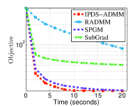
(a) w1a-2477-300

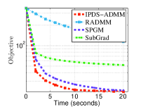
(b) TDT2-500-1000

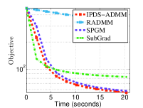
(c) 20News-8000-1000

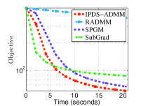
(d) sector-6412-100

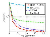
(e) w1a-2477-300

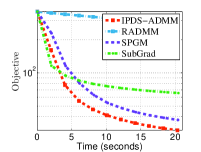
(f) TDT2-500-1000

(g) 20News-8000-1000

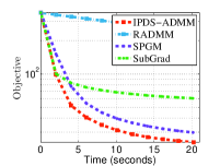
(h) sector-6412-100

Figure 2: The convergence curve of the compared methods for solving sparse PCA with $\rho^{\prime}=1$.

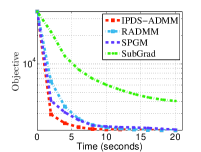
(a) w1a-2477-300

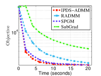
(b) TDT2-500-1000

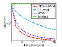
(c) 20News-8000-1000

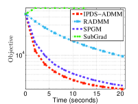
(d) sector-6412-100

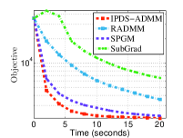
(e) w1a-2477-300

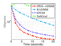
(f) TDT2-500-1000

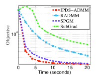
(g) 20News-8000-1000

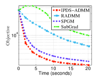
(h) sector-6412-100

Figure 3: The convergence curve of the compared methods for solving sparse PCA with $\rho^{\prime}=100$.

Appendix D Additional Experiment Details and Results

We offer further experimental details in Sections D.1 and D.2, and include additional results in Section D.3.

D.1 Datasets

We incorporate six datasets in our experiments, which include both randomly generated data and publicly available real-world data. These datasets serve as our data matrices $\mathbf{D}\in\mathbb{R}^{m^{\prime}\times d^{\prime}}$. The dataset names are as follows: ‘CnnCaltech-$m^{\prime}$-$d^{\prime}$’, ‘TDT2-$m^{\prime}$-$d^{\prime}$’, ‘sector-$m^{\prime}$-$d^{\prime}$’, ‘mnist-$m^{\prime}$-$d^{\prime}$’, ‘randn-$m^{\prime}$-$d^{\prime}$’, and ‘dct-$m^{\prime}$-$d^{\prime}$’. Here, ${{\rm{randn}}(m,n)}$ represents a function that generates a standard Gaussian random matrix with dimensions $m\times n$, while ${\rm{dct}}(m,n)$ refers to a function that produces a random matrix sampled from the discrete cosine transform. The matrix $\mathbf{D}\in\mathbb{R}^{m^{\prime}\times d^{\prime}}$ is constructed by randomly selecting $m^{\prime}$ examples and $d^{\prime}$ dimensions from the original real-world dataset (http://www.cad.zju.edu.cn/home/dengcai/Data/TextData.html,https://www.csie.ntu.edu.tw/~cjlin/libsvm/). We normalize each column of $\mathbf{D}$ to have a unit norm and center the data by subtracting the mean.

D.2 Projection on Orthogonality Constraints

When $h({\mathbf{x}})=\mathcal{I}_{\mathcal{M}}({\rm{mat}}({\mathbf{x}}))$, computing the proximal operator reduces to the following optimization problem:

$$\textstyle\bar{{\mathbf{x}}}\in\arg\min_{{\mathbf{x}}}\tfrac{\mu}{2}\|{\mathbf{x}}-{\mathbf{x}}^{\prime}\|_{2}^{2},\,s.t.\,{\rm{mat}}({\mathbf{x}})\in\mathcal{M}\triangleq\{\mathbf{V}\,|\,\mathbf{V}^{\mathsf{T}}\mathbf{V}=\mathbf{I}\}.$$

This is the nearest orthogonality matrix problem, and the optimal solution can be computed as $\bar{{\mathbf{x}}}={\rm{vec}}(\hat{\mathbf{U}}\hat{\mathbf{V}}^{\mathsf{T}})$, where ${\rm{mat}}({\mathbf{x}}^{\prime})=\hat{\mathbf{U}}{\rm{Diag}}(\mathbf{s})\hat{\mathbf{U}}^{\mathsf{T}}$ is the singular value decomposition of the matrix ${\rm{mat}}({\mathbf{x}}^{\prime})$. Please refer to [19].

D.3 Additional Experiment Results

We present the convergence curves of the compared methods for solving sparse PCA with $\rho^{\prime}=1$ and $\rho^{\prime}=100$ in Figures 3 and 3, respectively. It is evident that the proposed IPDS-ADMM generally outperforms other methods in terms of speed for the sparse PCA problem. These results further corroborate our earlier findings.

References

- [1] Rina Foygel Barber and Emil Y Sidky. Convergence for nonconvex admm, with applications to ct imaging. Journal of Machine Learning Research, 25(38):1–46, 2024.
- [2] Amir Beck. First-order methods in optimization. SIAM, 2017.
- [3] Dimitri Bertsekas. Convex optimization algorithms. Athena Scientific, 2015.
- [4] Fengmiao Bian, Jingwei Liang, and Xiaoqun Zhang. A stochastic alternating direction method of multipliers for non-smooth and non-convex optimization. Inverse Problems, 37(7):075009, 2021.
- [5] Radu Ioan Bo, Erno Robert Csetnek, and Dang-Khoa Nguyen. A proximal minimization algorithm for structured nonconvex and nonsmooth problems. SIAM Journal on Optimization, 29(2):1300–1328, 2019.
- [6] Radu Ioan Bo and Dang-Khoa Nguyen. The proximal alternating direction method of multipliers in the nonconvex setting: convergence analysis and rates. Mathematics of Operations Research, 45(2):682–712, 2020.
- [7] Axel Böhm and Stephen J. Wright. Variable smoothing for weakly convex composite functions. Journal of Optimization Theory and Applications, 188(3):628–649, 2021.
- [8] Radu Ioan Boţ, Minh N Dao, and Guoyin Li. Inertial proximal block coordinate method for a class of nonsmooth sum-of-ratios optimization problems. SIAM Journal on Optimization, 33(2):361–393, 2023.
- [9] Weiqiang Chen, Hui Ji, and Yanfei You. An augmented lagrangian method for -regularized optimization problems with orthogonality constraints. SIAM Journal on Scientific Computing, 38(4):B570–B592, 2016.
- [10] Damek Davis and Dmitriy Drusvyatskiy. Stochastic model-based minimization of weakly convex functions. SIAM Journal on Optimization, 29(1):207–239, 2019.
- [11] Wei Deng, Ming-Jun Lai, Zhimin Peng, and Wotao Yin. Parallel multi-block admm with o (1/k) convergence. Journal of Scientific Computing, 71:712–736, 2017.
- [12] Daniel Gabay and Bertrand Mercier. A dual algorithm for the solution of nonlinear variational problems via finite element approximation. Computers & mathematics with applications, 2(1):17–40, 1976.
- [13] Max LN Gonçalves, Jefferson G Melo, and Renato DC Monteiro. Convergence rate bounds for a proximal admm with over-relaxation stepsize parameter for solving nonconvex linearly constrained problems. arXiv preprint arXiv:1702.01850, 2017.
- [14] Max LN Gonçalves, Jefferson G Melo, and Renato DC Monteiro. Improved pointwise iteration-complexity of a regularized admm and of a regularized non-euclidean hpe framework. SIAM Journal on Optimization, 27(1):379–407, 2017.
- [15] Bingsheng He and Xiaoming Yuan. On the convergence rate of the douglas-rachford alternating direction method. SIAM Journal on Numerical Analysis, 50(2):700–709, 2012.
- [16] Le Thi Khanh Hien, Duy Nhat Phan, and Nicolas Gillis. Inertial alternating direction method of multipliers for non-convex non-smooth optimization. Computational Optimization and Applications, 83(1):247–285, 2022.
- [17] Mingyi Hong, Zhi-Quan Luo, and Meisam Razaviyayn. Convergence analysis of alternating direction method of multipliers for a family of nonconvex problems. SIAM Journal on Optimization, 26(1):337–364, 2016.
- [18] Feihu Huang, Songcan Chen, and Heng Huang. Faster stochastic alternating direction method of multipliers for nonconvex optimization. In International Conference on Machine Learning (ICML), volume 97, pages 2839–2848, 2019.
- [19] Rongjie Lai and Stanley Osher. A splitting method for orthogonality constrained problems. Journal of Scientific Computing, 58(2):431–449, 2014.
- [20] Hien Le, Nicolas Gillis, and Panagiotis Patrinos. Inertial block proximal methods for non-convex non-smooth optimization. In International Conference on Machine Learning, pages 5671–5681. PMLR, 2020.
- [21] Shuhuang Xiang Lei Yang, Xiaojun Chen. Sparse solutions of a class of constrained optimization problems. Mathematics of Operations Research, 2021.
- [22] Guoyin Li and Ting Kei Pong. Global convergence of splitting methods for nonconvex composite optimization. SIAM Journal on Optimization, 25(4):2434–2460, 2015.
- [23] Jiaxiang Li, Shiqian Ma, and Tejes Srivastava. A riemannian admm. arXiv preprint arXiv:2211.02163, 2022.
- [24] Min Li, Defeng Sun, and Kim-Chuan Toh. A majorized admm with indefinite proximal terms for linearly constrained convex composite optimization. SIAM Journal on Optimization, 26(2):922–950, 2016.
- [25] Xiao Li, Shixiang Chen, Zengde Deng, Qing Qu, Zhihui Zhu, and Anthony Man-Cho So. Weakly convex optimization over stiefel manifold using riemannian subgradient-type methods. SIAM Journal on Optimization, 31(3):1605–1634, 2021.
- [26] Qihang Lin, Runchao Ma, and Yangyang Xu. Complexity of an inexact proximal-point penalty method for constrained smooth non-convex optimization. Computational optimization and applications, 82(1):175–224, 2022.
- [27] Tian-Yi Lin, Shi-Qian Ma, and Shu-Zhong Zhang. On the sublinear convergence rate of multi-block admm. Journal of the Operations Research Society of China, 3:251–274, 2015.
- [28] Tianyi Lin, Shiqian Ma, and Shuzhong Zhang. On the global linear convergence of the admm with multiblock variables. SIAM Journal on Optimization, 25(3):1478–1497, 2015.
- [29] Wei Liu, Xin Liu, and Xiaojun Chen. Linearly constrained nonsmooth optimization for training autoencoders. SIAM Journal on Optimization, 32(3):1931–1957, 2022.
- [30] Yuanyuan Liu, Fanhua Shang, Hongying Liu, Lin Kong, Licheng Jiao, and Zhouchen Lin. Accelerated variance reduction stochastic admm for large-scale machine learning. IEEE Transactions on Pattern Analysis and Machine Intelligence, 43(12):4242–4255, 2020.
- [31] Zhaosong Lu and Yong Zhang. An augmented lagrangian approach for sparse principal component analysis. Mathematical Programming, 135:149–193, 2012.
- [32] Zhaosong Lu and Yong Zhang. Sparse approximation via penalty decomposition methods. SIAM Journal on Optimization, 23(4):2448–2478, 2013.
- [33] Renato DC Monteiro and Benar F Svaiter. Iteration-complexity of block-decomposition algorithms and the alternating direction method of multipliers. SIAM Journal on Optimization, 23(1):475–507, 2013.
- [34] Boris S. Mordukhovich. Variational analysis and generalized differentiation i: Basic theory. Berlin Springer, 330, 2006.
- [35] Y. E. Nesterov. Introductory lectures on convex optimization: a basic course, volume 87 of Applied Optimization. Kluwer Academic Publishers, 2003.
- [36] Robert Nishihara, Laurent Lessard, Ben Recht, Andrew Packard, and Michael Jordan. A general analysis of the convergence of admm. In International Conference on Machine Learning, pages 343–352. PMLR, 2015.
- [37] Yuyuan Ouyang, Yunmei Chen, Guanghui Lan, and Eduardo Pasiliao Jr. An accelerated linearized alternating direction method of multipliers. SIAM Journal on Imaging Sciences, 8(1):644–681, 2015.
- [38] Duy Nhat Phan and Nicolas Gillis. An inertial block majorization minimization framework for nonsmooth nonconvex optimization. Journal of Machine Learning Research, 24:1–41, 2023.
- [39] Thomas Pock and Shoham Sabach. Inertial proximal alternating linearized minimization (ipalm) for nonconvex and nonsmooth problems. SIAM Journal on Imaging Sciences, 9(4):1756–1787, 2016.
- [40] R. Tyrrell Rockafellar and Roger J-B. Wets. Variational analysis. Springer Science & Business Media, 317, 2009.
- [41] Li Shen, Wei Liu, Ganzhao Yuan, and Shiqian Ma. Gsos: Gauss-seidel operator splitting algorithm for multi-term nonsmooth convex composite optimization. In International Conference on Machine Learning, pages 3125–3134. PMLR, 2017.
- [42] Kaizhao Sun and Xu Andy Sun. Algorithms for difference-of-convex programs based on difference-of-moreau-envelopes smoothing. INFORMS Journal on Optimization, 5(4):321–339, 2023.
- [43] Quoc Tran Dinh. Non-ergodic alternating proximal augmented lagrangian algorithms with optimal rates. Advances in Neural Information Processing Systems, 31, 2018.
- [44] Junxiang Wang, Fuxun Yu, Xiang Chen, and Liang Zhao. ADMM for efficient deep learning with global convergence. In ACM International Conference on Knowledge Discovery & Data Mining (SIGKDD), pages 111–119, 2019.
- [45] Yu Wang, Wotao Yin, and Jinshan Zeng. Global convergence of admm in nonconvex nonsmooth optimization. Journal of Scientific Computing, 78(1):29–63, 2019.
- [46] Yi Xu, Mingrui Liu, Qihang Lin, and Tianbao Yang. Admm without a fixed penalty parameter: Faster convergence with new adaptive penalization. In Advances in Neural Information Processing Systems, volume 30. Curran Associates, Inc., 2017.
- [47] Lei Yang, Ting Kei Pong, and Xiaojun Chen. Alternating direction method of multipliers for a class of nonconvex and nonsmooth problems with applications to background/foreground extraction. SIAM Journal on Imaging Sciences, 10(1):74–110, 2017.
- [48] Maryam Yashtini. Multi-block nonconvex nonsmooth proximal admm: Convergence and rates under kurdyka–ojasiewicz property. Journal of Optimization Theory and Applications, 190(3):966–998, 2021.
- [49] Maryam Yashtini. Convergence and rate analysis of a proximal linearized ADMM for nonconvex nonsmooth optimization. Journal of Global Optimization, 84(4):913–939, 2022.
- [50] Jinshan Zeng, Shao-Bo Lin, Yuan Yao, and Ding-Xuan Zhou. On ADMM in deep learning: Convergence and saturation-avoidance. Journal of Machine Learning Research, 22:199:1–199:67, 2021.
- [51] Jinshan Zeng, Wotao Yin, and Ding-Xuan Zhou. Moreau envelope augmented lagrangian method for nonconvex optimization with linear constraints. Journal of Scientific Computing, 91(2):61, 2022.
- [52] Jiawei Zhang and Zhi-Quan Luo. A proximal alternating direction method of multiplier for linearly constrained nonconvex minimization. SIAM Journal on Optimization, 30(3):2272–2302, 2020.
- [53] Ruiliang Zhang and James Kwok. Asynchronous distributed admm for consensus optimization. In International Conference on Machine Learning, pages 1701–1709. PMLR, 2014.
- [54] Daoli Zhu, Lei Zhao, and Shuzhong Zhang. A first-order primal-dual method for nonconvex constrained optimization based on the augmented lagrangian. Mathematics of Operations Research, 2023.