Abstract
In this paper, we study the higher-order Beverton-Holt equation. We derive non trivial symmetries, and thereafter, solutions are obtained. For constant rate and carrying capacity, we study the periodic nature of the solution and analyze the stability of the equilibrium points have been analyzed.
Symmetry and Dynamical Analysis of a Discrete Time Model: The Higher Order Berverton-Holt Equation
Mensah Folly-Gbetoula ***Author: Mensah.Folly-Gbetoula@wits.ac.za
School of Mathematics, University of the Witwatersrand, Wits 2050, Johannesburg, South Africa.
2000 Mathematics Subject Classification: 76M60, 39A05, 39A11
Keywords: Difference equation, symmetry, reduction, group invariant, periodic solution
1 Introduction
Population studies is a scientific study of animal and human populations. More often, this study involves parameters that are highly connected to the age, gender, geographic distribution as well as the evolution of the population understudy. Many models have been developed: logistic model, the Ricker model, the Beverton-Holt model, etc. The latter was first introduced in the topic of fisheries by Berverton and Holt in the twentieth century and is known to be [1]
where are respectively, the carrying capacity and the inherent growth rate.
Later, many authors were attracted by the periodically forced nonautonomous delay higher-order Beverton-Holt model [2]
| (1.1) |
where , are non-negative -periodic sequences and the initial conditions , are all positive and interesting results were obtained.
In this work, we study the invariance properties of (1.1) and we construct its solutions via the invariant of their group of transformations. As one would expect, the study of existence of periodic solutions and the stability character of the solutions becomes easier once the form of the solutions are known. Higher-order difference equations have been studied from different angles by many researchers [3, 4, 5, 6, 9, 10, 12].
1.1 Preliminaries
For a deeper knowledge of symmetry analysis of recurrence equations, one can refer to [8] from which most of our notation and theorems are picked. To start, let be some continuous variables in a given differential equation and
be a (local) point transformations.
Definition 1.1.
A parameterized set of transformations
| (1.2) |
is a one-parameter local Lie group of transformations if the set of conditions below is satisfied:
-
1.
is the identity map, so that when .
-
2.
for every sufficiently close to .
-
3.
Every can be represented as a Taylor series in , that is,
Definition 1.2.
The infinitesimal generator of the one-parameter Lie group of point transformations (1.2) is the operator
| (1.3) |
and is the gradient operator.
Theorem 1.1.
is invariant under the Lie group of transformations (1.2) if and only if
| (1.4) |
Consider a forward difference equation
| (1.5) |
of order where is a regular domain. We strive to find a Lie group of point transformations
| (1.6) |
Observe that is the group parameter and is the characteristic of the group of transformations. Let
| (1.7) |
be the prolonged generator admitted by the group of point transformations (1.6). Then the invariance condition reads
| (1.8) | ||||
subject to (1.5). Symmetries are powerful tools for reduction of order of differential and difference equations. In this paper, the reduction of order will be achieved using symmetries and the well-known canonical coordinate [11].
| (1.9) |
Definition 1.3.
The equilibrium point of (1.5) is stable (locally) if
| (1.10) |
for all solutions of (1.5).
Definition 1.4.
Definition 1.5.
Theorem 1.2.
Suppose is a smooth function defined on some neighborhood of . Then,
-
(i)
If all the roots, , of (1.11) are such that , then the equilibrium point is locally asymptotically stable.
- (ii)
Definition 1.6.
Theorem 1.3.
Suppose the ’s are real numbers satisfying
Then, the roots of (1.11) lie inside the open unit disk .
2 Main results
2.1 Symmetries
For the sake of aesthetics, we rewrite the Beverton-holt equation as
| (2.1) |
with
| (2.2) |
In the Beverton-Holt model, is set to be greater than one. This implies that should be less that one. In this paper, we investigate solutions that are mathematically correct, so without loss of generality, we will will assume that is simply a real number. Seeking for Lie symmetries, we force the criterion of invariance (1.8) on (1.1). This yields
| (2.3) |
Solving the functional equation above, we obtain (after a set of lengthy computations) the infinitesimals:
-
()
(2.4) where , that is to say,
(2.5) -
()
(2.6) where , that is to say,
(2.7) -
()
(2.8) where and , that is to say,
(2.9) and
(2.10) with and .
Using these infinitesimals, we obtain the following symmetries:
| (2.11) | ||||
| (2.12) | ||||
| (2.13) |
where and are given in equations (2.5), (2.7), (2.9) and (2.10), respectively.
2.2 Canonical coordinate closed form solution
We select the infinitesimal to lower the order (1.1). Thus, the canonical coordinate takes the form
| (2.14) | ||||
| (2.15) |
and therefore
| (2.16) | ||||
| (2.17) |
Setting , we find that
| (2.18) |
and we take notice of
| (2.19) |
By iterating (2.18), we get
| (2.20) |
for . We reverse the order created by the change of variables to derive the solution of (1.1). We observe from (2.19) that
from which we obtain
| (2.21) |
Recall that and . So, the closed form solution to the Beverton-Bolt (1.1) is given by
| (2.22) |
provided the denominators are non-zero.
2.3 Periodicity in the growth rate and the carrying capacity
The goal of the next section is to investigate the form of the solution when the growth rate and the carrying capacity are 1 or - periodic sequences.
2.3.1 The case when and are -periodic
2.3.2 The case when and are 1-periodic (constant)
2.4 Periodicity in the solution and analysis of the stability of the equilibrium points
In this section, we investigate the existence of periodic solutions and the nature of the equilibrium points of the model under study. We demonstrate that periodic solutions do exist under certain restrictions.
Theorem 2.1.
The solution of
| (2.26) |
where , is -periodic if and only the following conditions are met:
-
(i)
The sequence and periodic with period .
-
(ii)
The initial conditions, , satisfy .
Proof.
Suppose the initial conditions satisfy the conditions . Using the latter in (2.3.1), we have that:
| (2.27) |
It follows is periodic with period divisible by . With the choice of the restriction on the initial conditions, the period can not be less that . Therefore, is periodic with period . ∎
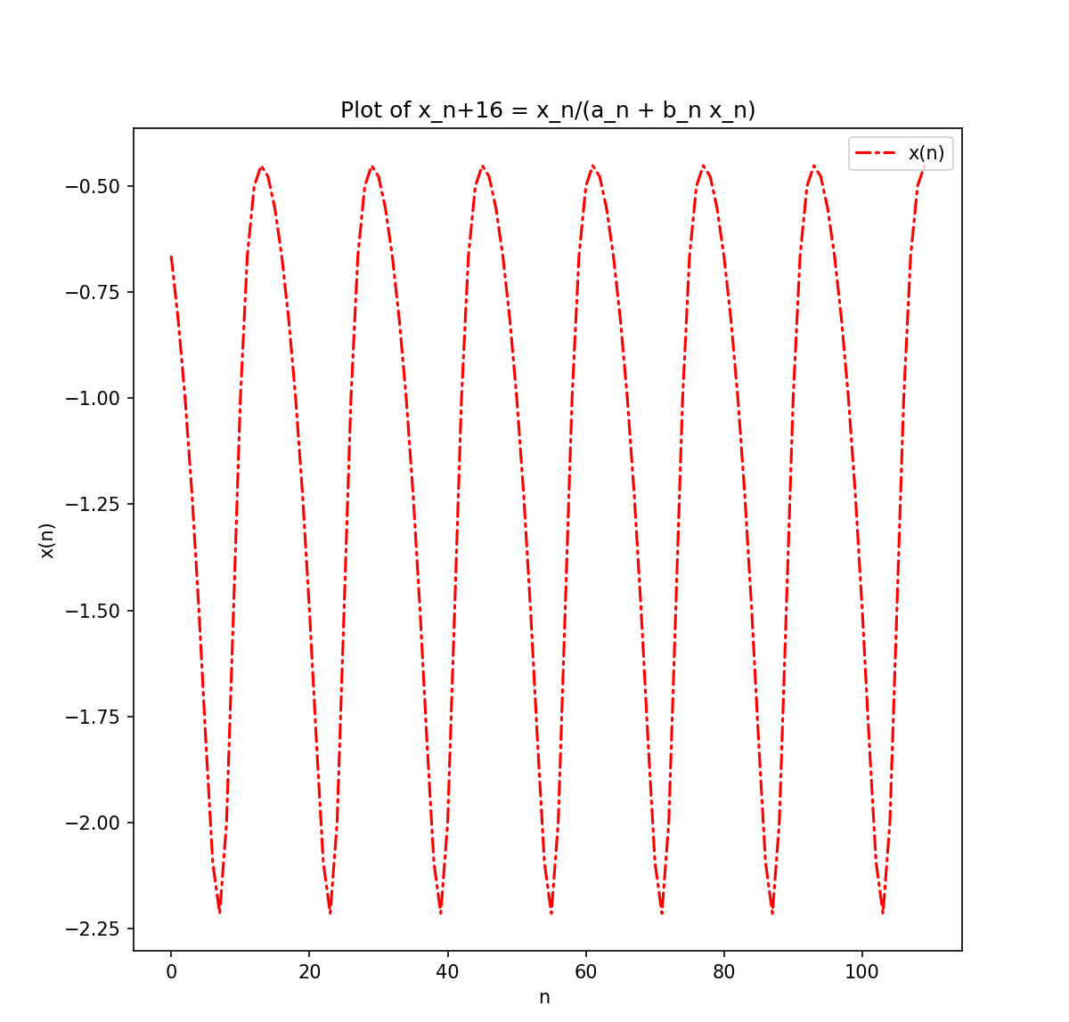
In Figure 2, we used the initial conditions
. These initial conditions satisfy the conditions in Theorem 2.1. As predicted, we have -periodic solutions.
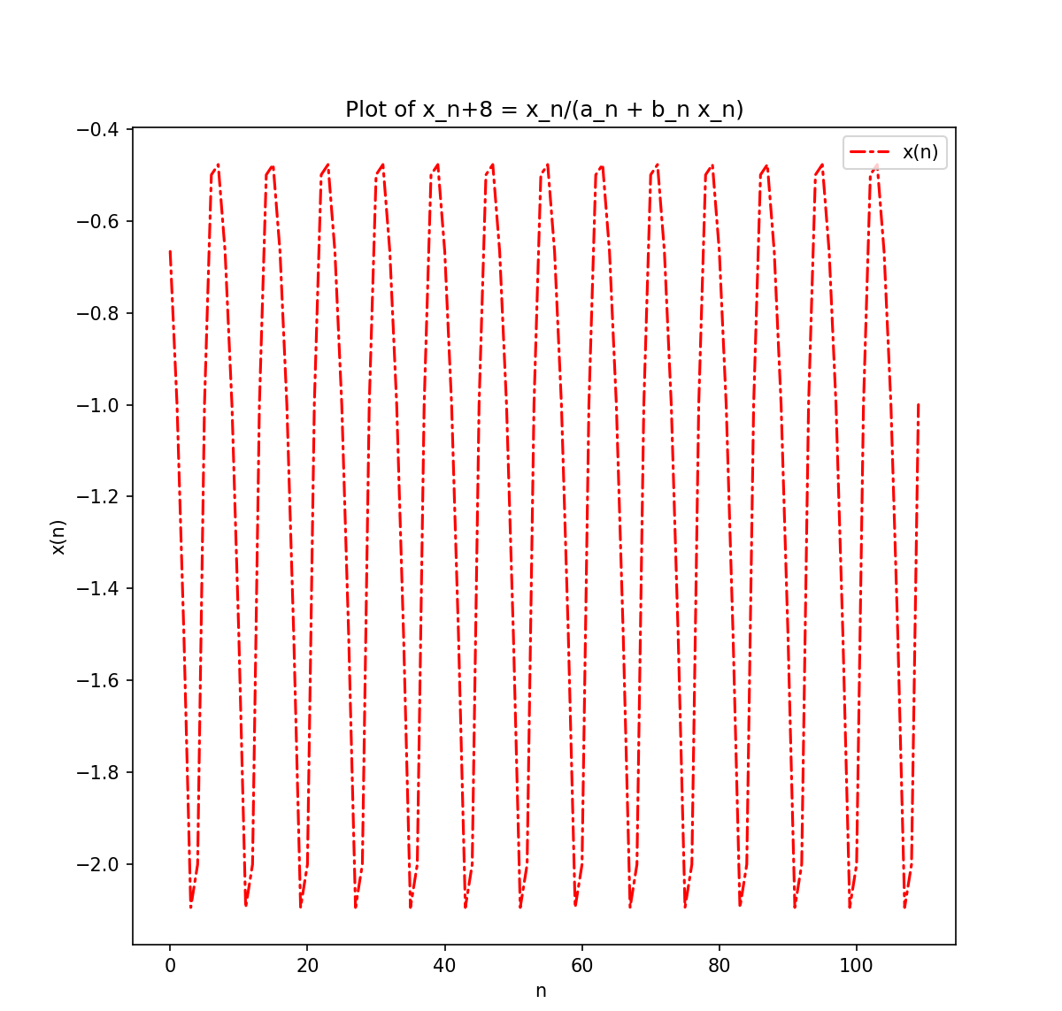
In Figure 2, we used the initial conditions
. These initial conditions satisfy the conditions in Theorem 2.1. As predicted, we have -periodic solutions.
Theorem 2.2.
The solution of
| (2.28) |
where , is -periodic if and only the initial conditions, , satisfy .
Proof.
The proof is identical to the proof of Theorem 2.1 and is omitted. ∎
Theorem 2.3.
The solution of
| (2.29) |
is periodic and contains two cycles of length .
Proof.
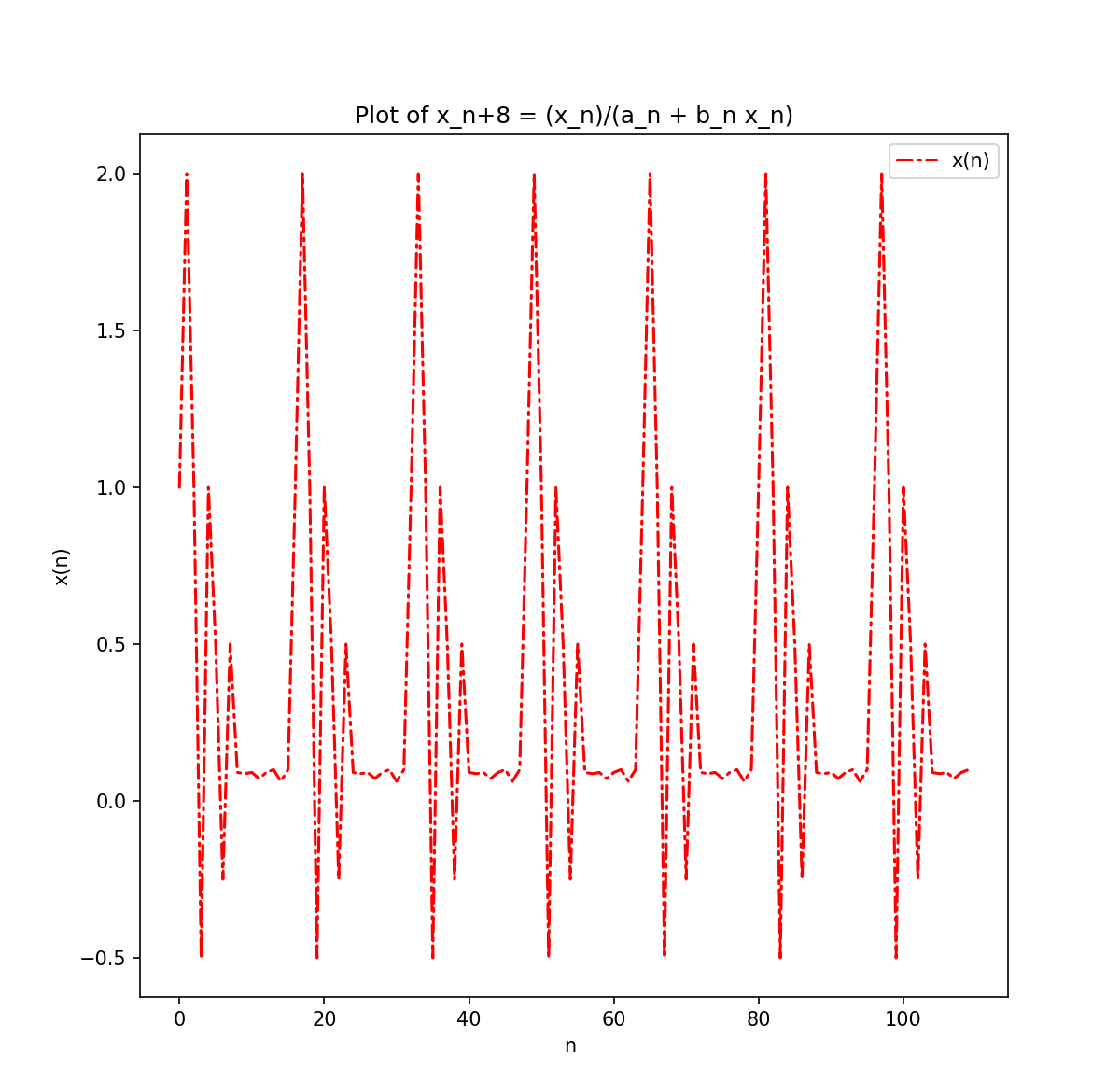
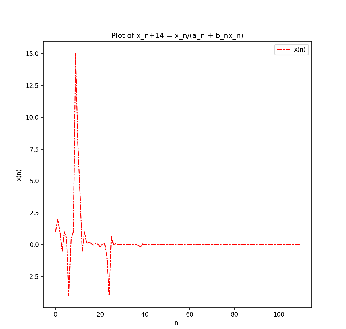
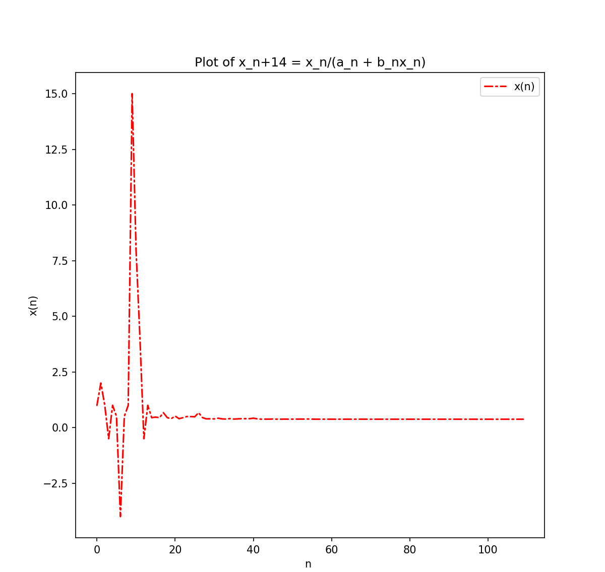
In Figure 4, we used the initial conditions . As predicted, we have -periodic solutions.
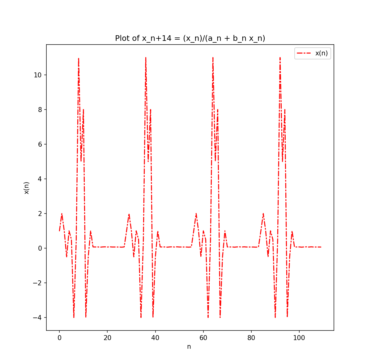
In Figure 4, we used the initial conditions . As predicted, we have -periodic solutions.
Theorem 2.4.
Proof.
The equilibrium points of (1.1) are the solutions of the equation . If we let
| (2.33) |
then:
-
-
For , it is easy to see that and so, the characteristic equation of (1.1) around this equilibrium point is given by It follows that when , in order words, is locally asymptotically stable. On the other hand, when or in order words, unstable.
-
-
For , and the characteristic equation of (1.1) around this equilibrium point is . Consequently, when , the roots ’s of this characteristic equation are such that and therefore the equilibrium is asymptotically stable in this case. Similarly, when , the moduli of the roots are greater than one and therefore the equilibrium is unstable in this case.
∎
Theorem 2.5.
If , then the equilibrium point of (1.1) is non-hyperbolic.
3 Conclusion
We performed the invariance analysis of the higher-order Beverton-Holt difference equation. Symmetries and the formula solutions are presented. We utilized the canonical coordinate to derive invariants that have been used reduce linearize the equation and eventually obtained the solutions in closed form. We have also presented periodic solutions that satisfy certain ansatz. Lastly, we studied the stability of the equilibrium points of the model.
References
- [1] Ray J.H. Beverton, Sidney J. Holt, On the Dynamics of Exploited Fish Populations, Fish. Invest. (Great Britain, Ministry of Agriculture, Fisheries, and Food), vol.19&29, H. M. Stationery Off., London, 1957.
- [2] M. Bohnera, F. M.Dannanb and S. Streiperta, A nonautonomous Beverton?Holt equation of higher order, J. Math.Anal.Appl. 457 (2018), 114 – 133.
- [3] E. M. Elsayed, Solution and Attractivity for a Rational Recursive Sequence, Discrete Dynamics in Nature and Society, 2011 (2011) Article ID 982309, 17 pages.
- [4] M. Folly-Gbetoula, Symmetry, reductions and exact solutions of the difference equation ,J. Diff. Equations and Applications, 23:6 (2017) 1017-1024.
- [5] M. Folly-Gbetoula and A.H. Kara, Symmetries, conservation laws, and integrability of difference equations, Advances in Difference Equations, 2014, 2014.
- [6] M. Folly-Gbetoula, Kgatliso Mkhwanazi and D. Nyirenda, On a study of a family of higher order recurrence relations, Mathematical Problems in Engineering 2022 (2022), Article ID 6770105, 11 pages.
- [7] Grove, E. A.; Ladas, G. Periodicities in Nonlinear Difference Equations, Vol. 4; Chapman & Hall/CRC: Boca Raton, USA, 2005.
- [8] P. E. Hydon, Difference Equations by Differential Equation Methods, Cambridge University Press (2014).
- [9] T. F. Ibrahim, On the third order rational difference equation , Int. J. Contemp. Math. Sciences 4:27 (2009), 1321-1334.
- [10] R. Karatas, On the solutions of the recursive sequence , Selcuk J. Appl. Math., 9:2 (2008) 3-8.
- [11] S. Maeda, The Similarity Method for Difference Equations, IMA Journal of Applied Mathematics, 38 (1987), 129-134.
- [12] I. Yalcinkaya, On the global attractivity of positive solutions of a rational difference equation, Selcuk J. Appl. Math., 9:2 (2008) 3-8.