Computational Efficient Width-Wise Early Exits in Modulation Classification

Abstract

Deep learning (DL) techniques are increasingly pervasive across various domains, including wireless communication, where they extract insights from raw radio signals. However, the computational demands of DL pose significant challenges, particularly in distributed wireless networks like Cell-free networks, where deploying DL models on edge devices becomes hard due to heightened computational loads. These computational loads escalate with larger input sizes, often correlating with improved model performance. To mitigate this challenge, Early Exiting (EE) techniques have been introduced in DL, primarily targeting the depth of the model. This approach enables models to exit during inference based on specified criteria, leveraging entropy measures at intermediate exits. Doing so makes less complex samples exit early, reducing computational load and inference time. In our contribution, we propose a novel width-wise exiting strategy for Convolutional Neural Network (CNN)-based architectures. By selectively adjusting the input size, we aim to regulate computational demands effectively. Our approach aims to decrease the average computational load during inference while maintaining performance levels comparable to conventional models. We specifically investigate Modulation Classification, a well-established application of DL in wireless communication. Our experimental results show substantial reductions in computational load, with an average decrease of 28%, and particularly notable reductions of 65% in high-SNR scenarios. Through this work, we present a practical solution for reducing computational demands in deep learning applications, particularly within the domain of wireless communication.

I Introduction

Recent advances in wireless communication show a shift towards distributed network paradigms, exemplified by emerging concepts like crowdsourced sensor networks [1] and cell-free networks [2]. Notably, in the development of 6th Generation (6G) mobile networks, there is a trend towards cell-free distributed deployments [3], aimed at mitigating path-loss effects and ensuring homogeneous signal-to-noise ratio (SNR) across all user locations.

This transition towards distributed networks also brings out a paradigm of distributed processing, which is essential for ensuring the scalability of such networks. Specifically, for Deep Learning (DL)-based applications, this distributed approach has spurred the development of learning strategies such as federated learning [4], split learning [5], and distributed inference strategies [6, 7], where individual devices either make local decisions or collaboratively generate a central decision.

This trend towards distributed processing relocates computation to the network edge, catering to devices with energy constraints or computational load restrictions. In a study by [8], the authors explore the application of Early Exiting (EE) techniques to DL-based Automatic Modulation Classification (AMC). This concept involves making classification decisions at intermediate classifiers, allowing some input samples to exit early, thereby reducing computational load and speeding up inference time. The main idea behind EE is that not all input samples require the same network depth to classify correctly.

Building upon the concept of EE, our proposed method focuses on reducing computational load during inference by segmenting input samples and processing each segment sequentially using corresponding expert models. At the classifier of each expert model, a decision is made to either accept the classification or delegate it to the next expert model. This width-wise implementation of early exiting enables us to tailor each expert model to target a specific subset of the dataset. Similar to the concept of EE, which shows that not all input samples need the full depth of the network for correct classification, our width-wise approach showcases correct classification can be achieved with a segment of the input sample.

We implement our approach for AMC, a pivotal technology introduced approximately 15 years ago as a key technology for wireless networks [9, 10] in the search towards more flexible and cognitive networks. Over the years, approaches in AMC have transitioned from statistical signal processing methods to DL-based models [11], with the ResNet architecture [12] widely recognized as one of the most performant feasible architectures. However, the high computational cost is often considered a barrier to implementing AMC in distributed and collaborative applications such as 6G Cell-free networks [6]. Our implementation aims to demonstrate width-wise EE, lay the groundwork for further research in this area, and does not aim to surpass the state-of-the-art accuracy in AMC.

I-A Contribution

This paper proposes and evaluates a novel approach to reduce the average computational load of Convolutional Neural Network (CNN)-based networks based on EE. To the best of our knowledge, this work leads the way in describing and discussing a width-wise implementation of EE as opposed to the commonly implemented depth-wise EE. The reasoning behind width-wise EE stems from the observation that the predominance computational load arises primarily from the initial convolutional layers before applying any pooling strategy. The computational load reduces significantly after each subsequent pooling operation as the features, which are the input of the subsequent convolutional layer, are reduced.

Another challenge addressed in this paper is the selection of an adaptive exit criterion. Initially, exit criteria are established post-training and fine-tuned to balance model accuracy and time/computational load reduction. This iterative process involves testing various thresholds to determine optimal behavior. While such an implementation is feasible when dealing with only one intermediate exit, it becomes cumbersome when considering multiple exits. We propose and implement an adaptive exit criterion based on entropy, which enables the specification of targeted accuracy and the percentage of exits at each expert model. The selection of the exit criterion is data-driven and tailored to the current model.

The main contribution of this paper is twofold.

• First, we propose a novel width-wise EE approach based on ResNet and apply this approach to AMC. To analyze the reduction in computational load, we compare the proposed model against a similar baseline model comprising a direct implementation of a ResNet model. We show that our approach uses around 28% less computations on average, peaking at 65% less computations at high-SNR input samples while maintaining a similar accuracy.

• Second, we propose a dynamic method for selecting exit criteria based on a target accuracy and exit percentage at each expert model. By enabling the specification of these targets, the trade-off between model accuracy and exit percentage becomes more intuitive when training an EE model. This is particularly crucial in the context of research focused on EE models featuring multiple exits.

The remainder of the paper is structured as follows. Section II outlines the signal model and the AMC problem statement. Section III introduces the architectures of the baseline and proposed model. Subsequently, we present the performance evaluation results in Section IV. Finally, the paper concludes with final remarks in Section V.

II Signal Model and Problem Statement

We consider a scenario where a single transmitter transmits a modulated signal $s(t)$ through a flat fading channel $h(t)$ comprising attenuation and additive white noise $v(t)$. The modulation format $m$ employed by the transmitter is chosen from a set of known modulations $\mathcal{M}$. Upon reception, the continuous signal $r(t)$, denoted in Eq. 1, is discretized into In-phase/Quadrature (IQ) samples. A collection of $N$ raw IQ samples forms a frame, represented as matrix $R$ with dimensions $(N,2)$, where each column corresponds to the $I$ and $Q$ values.

$$r(t)=s(t)\times h(t)+v(t)\,.$$ (1)

The objective of AMC is to correctly identify the transmitted modulation $\hat{m}$ from the known modulations $\mathcal{M}$ by analyzing the received signal according to a Maximum A Posteriori (MAP) criterion:

$$\hat{m}=\arg\max_{m\in\mathcal{M}}\mathbb{P}(m|\textbf{R})$$ (2)

III Architectures

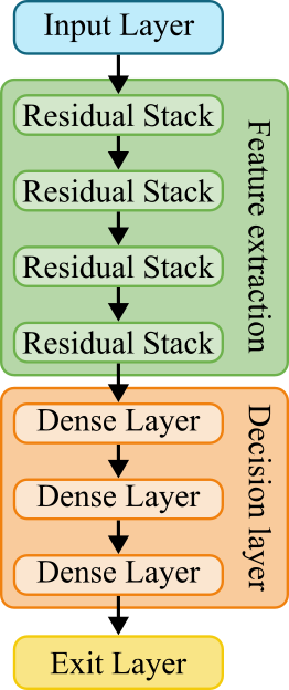
((a)) Baseline model, based on the ResNet model

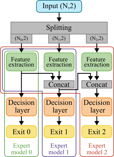
((b)) Proposed model containing 3 smaller expert models

Figure 1: Architecturs of the baseline and the proposed model.

In this paper, ResNets are the foundation of the baseline and proposed model. Fig. 1(a) offers a comprehensive overview of the ResNet model, systematically divided into four functional blocks for clarity in our discussion. Initially, we introduce the baseline model, providing detailed explanations of its four functional blocks. Subsequently, we delve into constructing the proposed model, covering its architectural development, training procedure, and inference method.

III-A Baseline model

The baseline model is a direct implementation of a ResNet model. The first block, the input layer, interfaces real-world data with the model. The input of this block is the IQ samples derived from the dataset. The output of this block is a vector of dimensions $N\times 2$, with $N$ corresponding to the number of IQ samples in each frame. The second block, dedicated to feature extraction, consists of multiple residual stacks. The received IQ samples are transformed into features using these residual stacks. The number of residual stacks is a design parameter, where each stack consists of 32 filters with a (3,1) kernel. Upon feature extraction, the third block, referred to as the decision layer, forms a soft decision. The soft decision comprises the probability assigned by the decision layer to identify the modulation utilized in the input IQ samples. The decision layer comprises two dense layers with 128 neurons each and a dense layer with six neurons (representing each modulation under consideration). Finally, the fourth and last block, the exit layer, concludes the model’s prediction by selecting the modulation with the highest probability. This hierarchical organization of the ResNet model provides a structured framework for understanding its functionality and predictive capabilities. These four blocks are used in addition to two non-trainable blocks to build the proposed model.

III-B Proposed model

The aim of the proposed model is to reduce the average computational load while upholding the average classification accuracy. In traditional EE techniques, computational load reduction involves truncating the model’s depth and integrating exits in the depth dimension, allowing for layer skipping. However, for CNN-based models, where pooling layers are utilized to decrease feature numbers, the heaviest computational load often resides in the initial layers of the network. The proposed model addresses this issue by focusing on these initial layers, as computational load diminishes with reduced input size, which is made possible due to the convolution operation performed by CNNs.

The architecture of the proposed model is illustrated in Fig. 1(b). Following the input layer of the proposed model, a splitting layer divides the original input vector of size $N$ into segments. Each segment corresponds to a distinct subset of the input vector: the first segment encompasses the initial $N_{0}$ values, the second segment comprises the subsequent $N_{1}$ values, and the final segment encompasses the remaining $N_{2}$ values, with $N_{0}+N_{1}+N_{2}=N$.

After the splitting layer, the model branches into three distinct sub-models. Each sub-model is tailored to address a specific subset of the dataset, classifying frames based on their difficulty level categorized as easy, medium, or hard. It is noteworthy that this categorization is automatically conducted by the model. Subsequent analysis reveals that the categorization closely aligns with factors such as the modulation type and SNR of the frames. Consequently, each sub-model specializes in classifying a particular subset of data, effectively becoming an expert model.

Each expert model comprises three main components: a feature extraction layer, a decision layer, and an exit layer. During feature extraction, the model utilizes a specified number of residual stacks, each consisting of 32 filters with a (3,1) kernel. Following feature extraction, the decision layer of each expert model consists of two dense layers, each with 128 neurons and a dense layer containing six neurons.

In the case of subsequent expert models, features extracted from previous segments by the corresponding expert are also considered. This is achieved by concatenating these features with the features extracted from the current segment, ensuring that the model integrates information from previous segments seamlessly.

III-C Proposed Model Training

Training the proposed model unfolds into two phases. In the first phase, the joint phase, the whole model is jointly trained on all the training frames of the dataset. To this end, we adapt the loss function proposed in [13] with all weights set to one. This loss function is, therefore, the sum of the categorical loss at each exit of the model given by Eq. 3.

$$L_{joint}(\hat{\textbf{y}},\textbf{y};\theta)=\sum_{e=0}^{2}L(\hat{\textbf{y}}_{e},\textbf{y};\theta)$$ (3)

 

Each expert model is individually and sequentially retrained in the second training phase, starting with expert model 0. The second training phase consists of two steps. In the first step, one expert model is retrained using (a subset of) the training frames of the dataset. Upon retraining completion, the weights of this expert model are frozen, rendering them no longer trainable.

The second training phase’s second step determines an exit criterion using the training frames. Once an exit criterion is selected, the training frames are divided into two subsets: frames that would exit at this point and frames that would not. Frames that exit are excluded from further training steps, while the remaining frames are used to retrain the subsequent expert model. No exit criterion is selected for the last expert model, as all remaining frames exit at this stage.

By the end of the second training phase, the three expert models specialize in extracting distinct subsets of the dataset. Expert model 0 targets easy frames, expert model 1 handles medium frames, and the final expert model processes all frames that have not exited yet. Consequently, the dataset is divided into three subsets accordingly. After the second training phase, the model is completely trained, and the exit criterion at each exit is dynamically determined.

III-D Proposed Model Inference

During inference, the objective is to classify the modulation of an unseen frame. Initially, the frame is segmented into segments corresponding to each expert model. Expert model 0 initiates the process by processing the first segment. Based on the entropy, calculated from the soft decision, and an exit criterion learned during training, Expert model 0 decides whether to classify the frame immediately or delegate the classification to the next expert model.

If expert model 0 delegates the classification, expert model 1 begins processing its corresponding segment of the unseen frame. Upon completing the feature extraction layer, the extracted features from expert model 0 are concatenated with those from expert model 1. Similarly, at the decision layer, expert model 1 determines whether to classify the frame or delegate the classification to the final expert model based on the exit criterion obtained.

Should expert model 1 choose to delegate the classification, the final expert model 2 performs the classification based on the features extracted from the final segment and those extracted by the two preceding expert models. The final expert model 2 cannot delegate the classification further and proceeds to classify the frame. When an expert model decides to classify, the objective is achieved, and no further processing is done. This results in a lower computational load when classifying at an earlier than a later exit.

III-E Exit Criterion Selection

At each exit, except for the final one, we derive an exit criterion based on the cross-categorical entropy of the soft decision (Z) as defined in Eq. 4. Here, $z_{i}$ represents the confidence level of each classification class obtained from the soft decision made by the decision layer.

$$H(\textbf{Z})=\sum_{i=0}^{5}-z_{i}log_{2}(z_{i}).$$ (4)

Selecting an appropriate threshold entropy results in the trade-off between classification accuracy and computational load reduction. Fig. 2 illustrates the relationship between accuracy and the percentage of frames exiting based on different threshold entropy values. It is important to note that the classification accuracy is calculated only for the subset of data that exits at the specified threshold. The figure shows that accuracy decreases as the threshold entropy increases while the percentage of exiting frames rises. To determine the threshold, we employ two key considerations as follows.

• We first identify the entropy $H_{Acc}$ at which the accuracy drops below a predetermined percentage. We opt for a threshold of 95%, ensuring that frames exiting at this point are classified with a sufficiently high accuracy. Lowering this threshold may result in a notable decrease in overall model accuracy.

• Next, we select the threshold $H_{exits}$ at which at least 35% of the training frames are exiting. Choosing a lower $H_{exits}$ value may underutilize the exit, resulting in a less substantial reduction in computational load.

Finally, we compute the average of these two selected values to establish the exit criterion $H_{th}$. The selection of the desired accuracy (95%) and exit percentage (35%) is based on empirical analysis, representing a trade-off between achieving high accuracy and optimizing exit efficiency, which results in a lower computational load.

Figure 2: Exit threshold selection by averaging the entropy where the accuracy drops below 95% and the entropy for which at least 35% of the training frames exit.

IV Results and discussion

To mitigate the impact of randomness inherent in deep learning when dealing with a limited-size dataset, we conduct 32 Monte Carlo simulations and average the results for both the baseline and the proposed model. The baseline model undergoes training for 40 epochs in each simulation, employing early stopping based on validation frames. Similarly, the proposed model undergoes training with 40 epochs per training step and early stopping.

We quantify the performance of both the proposed model and the baseline model using two key metrics: model accuracy and computational load, which are defined as follows.

• Model accuracy represents the percentage of correctly classified modulation schemes. A higher accuracy value indicates better performance.

• Computational load is evaluated by the number of floating-point operationsrequired for a model to perform one modulation classification. A lower FLOP count indicates a reduced computational burden. We estimate FLOPs using TensorFlow’s built-in estimator. However, it is important to note that these estimates serve as approximations and may vary depending on hardware configurations.

In the subsequent sections, we will initially present the dataset created for the results, followed by an overview of the model design parameters and, ultimately, a comparison between the proposed and baseline models.

IV-A Dataset

A synthetic dataset is generated based upon the recently released RML22 [14], using Python and gnuradio [15]. Our dataset considers six different modulation techniques $\mathcal{M}=\{$BPSK , QPSK, PSK8, PAM4, QAM16, QAM64 $\}$. The SNR of the signal chosen ranges from $-20dB$ to $20dB$ with a step of $2dB$, resulting in 21 different SNRs. For each pair of modulation and SNR, we generated 1024 frames of 1024 IQ samples. To ensure an equal representation of each SNR/Modulation pair, the dataset is split by randomly picking 768 frames for training, 128 frames for validation, and the remaining 128 frames for testing for each SNR/modulation pair. This resulted in a total of 112,880 frames, of which 98,304 were used for training, 12,288 for validation, and the final 12,288 for testing.

IV-B Model Design Parameters

To maintain the comparability between the baseline and proposed models, both models utilize an input size of (512,2), representing a vector of IQ samples. We adopt a configuration consisting of 4 residual stacks for the baseline model’s feature extraction. Similarly, each feature extraction layer in the proposed model, mirroring the baseline structure, encompasses four residual stacks, effectively partitioning the baseline’s feature layer into three segments. Ensuring parity in computational complexity, as the total computational workload for feature extraction in the baseline model matches the cumulative workload across all feature extraction layers in the proposed model.

While the proposed model introduces additional design parameters, we uphold consistency in the input vector size to facilitate a fair comparison. This input vector is split into three segments: the first segment comprises 32 IQ samples, 160 samples for the second segment, and the remaining 320 samples for the final segment.

IV-C Computational load

The computational load of the baseline model is fixed, while for the proposed model, the computational load depends on which exit has been taken. Either way, it is observed that around half of the Million FLOPs are used in calculating the first residual stack of each feature layer, emphasizing the motivation of the proposed width-wise EE model. Table I provides an overview of the amount of MFLOPs used for modulation classification at inference for the baseline model and at each expert model of the proposed model.

The selection of a small segment size for expert model 0 results in a computational requirement that is an order of magnitude lower than the baseline and the other expert models. Expert model 2, on the other hand, exhibits a slightly higher computational load compared to the baseline model. This is due to the intermediate checks performed by the expert models 0 and expert model 1. We also provide the amount of trainable parameters, which is usually linked with the model complexity. However, the number of parameters is not a good metric when comparing the computational load. Both the baseline model and Exit 1 have similar trainable parameters; however, the computational load of the baseline model is threefold.

TABLE I: MFLOPs and amount of trainable parameters for baseline model and each exit of the proposed model

	total MFLOPs	params
Baseline model	12.53	202 438
Expert model 0	0.80	79558
Expert model 1	4.73	200076
Expert model 2	12.62	402514

Figure 3: Computational load of the proposed and baseline model.

The average computational load is calculated by multiplying the computational load of each expert model by the percentage of frames exiting at the corresponding expert model. Fig. 3 illustrates the reduction in computational load achieved by the proposed model compared to the baseline model. For low-SNR scenarios, there is a minor increase in computational cost attributable to the intermediate checks. Conversely, for higher SNR values, the reduction in computational load is significant, reaching up to 65%. This graph demonstrates that the proposed model prioritizes the exiting of frames with higher SNR, generally regarded as easier samples. On average, across all SNR levels, the proposed model achieves a 28% reduction in computational load.

IV-D Classification accuracy

Figure 4: Reduction in computational load of the proposed model compared to the baseline model.

The classification accuracies for both the baseline and proposed models are depicted in Fig. 4. As anticipated, the accuracies exhibit a typical pattern, with lower accuracies observed at lower SNR, gradually increasing as SNR values rise. Notably, the accuracy reaches its peak at approximately 80% for SNRs exceeding 10 dB.

At higher SNRs, the proposed model consistently outperforms the baseline regarding accuracy. This improvement is elaborated in Table II, which compares performance metrics. The table shows the average accuracy across all 32 simulations for both models and the average accuracy of the 16 simulations with the highest and lowest accuracies. It becomes apparent that the proposed model demonstrates less variability in accuracy outcomes compared to the baseline model. This phenomenon can be attributed to the retraining process employed in the proposed model’s second training phase. Each expert model undergoes retraining during this phase, effectively addressing suboptimal performance and enhancing overall model consistency.

TABLE II: Mean accuracy of the 32 model simulations, the mean of the best 16 highest and 16 lowest simulation accuracies.

	Mean	Lowest 16	Highest 16
Baseline model	49.81%	45.47%	54.15%
Proposed model	50.90%	49.34%	52.45%

IV-E Early exiting frequency

In Fig. 5, the distribution of frame exits at various SNR levels is depicted, with each exit represented by a distinct color. Additionally, the figure distinguishes between correctly classified and misclassified frames for each exit. A noticeable trend emerges, indicating a correlation between frame SNR and exit selection. Higher SNR frames predominantly exit at earlier stages, while lower SNR frames are typically classified by the final expert model. Furthermore, the figure illustrates the dataset distribution into ’easy,’ ’medium,’ and ’hard’ subsets based on classification difficulty. It is important to note that the exit percentage is influenced not only by SNR but also by the modulation type. Thus, the efficacy of early exits varies depending on the dataset characteristics.

Table III provides detailed statistics for each exit, including the exit percentage and the accuracy of exited frames. These values can inform threshold selection to optimize model performance. Considering these metrics, tailoring the empirically chosen accuracy and exit percentage thresholds for each exit may be beneficial. Overall, only 35% of the frames exit early in the proposed model. Targeting a higher exit percentage may be advisable to reduce computational complexity further.

Figure 5: Frames per exit

TABLE III: The percentage of frames exiting at each exit and the corresponding classification accuracy of the exited frames.

	Exits	Accuracy
Expert model 0	20%	86.20%
Expert model 1	15%	75.35%
Expert model 2	65%	34.54%

V Conclusion and future work

This paper introduces and evaluates a novel EE strategy, utilizing width-wise model splitting to alleviate the average computational load. By targeting the computational impact of the initial layer, our proposed architecture achieves a notable reduction in computational load averaging 28%. Notably, the proposed model exhibits expected behavior, demonstrating lower computational loads for higher SNR levels, with reductions of up to 65%.

Moreover, this paper proposes a method for dynamically selecting an exit criterion based on the training data by selecting a targeted accuracy and percentage of exiting frames. This method can automate the threshold selection across different instantiations of the proposed model, which can be of special interest to edge computing.

Future research can focus on optimizing width-wise EE and exploring its applications across diverse domains. In the AMC realm, there is potential for enhancing performance in low-SNR scenarios. Low-SNR frames impose a significant computational load without significantly contributing to accuracy. Potential optimizations may include sample rejection or redirection to models specialized in handling low-SNR samples. Overall, the findings presented here contribute to the ongoing discourse in deep learning and modulation classification, offering insights and avenues for further exploration in optimizing computational load and model accuracy.

References

- [1] S. Rajendran et al., “Electrosense: Open and big spectrum data,” IEEE Communications Magazine, vol. 56, no. 1, pp. 210–217, 2017.
- [2] S. Chen, J. Zhang, J. Zhang, E. Björnson, and B. Ai, “A survey on user-centric cell-free massive mimo systems,” Digital Communications and Networks, 2021.
- [3] E. Bertilsson, O. Gustafsson, and E. G. Larsson, “A scalable architecture for massive mimo base stations using distributed processing,” in 2016 50th Asilomar Conference on Signals, Systems and Computers, pp. 864–868, 2016.
- [4] P. Kairouz, H. B. McMahan, B. Avent, and etc, “Advances and open problems in federated learning,” Foundations and Trends® in Machine Learning, vol. 14, no. 1–2, pp. 1–210, 2021.
- [5] J. Park, S. Oh, and S.-L. Kim, “Splitamc: Split learning for robust automatic modulation classification,” in 2023 IEEE 97th Vehicular Technology Conference (VTC2023-Spring), pp. 1–6, 2023.
- [6] D. Verbruggen, H. Salluoha, and S. Pollin, “Distributed deep learning for modulation classification in 6g cell-free wireless networks,” 2024.
- [7] C. Hu and B. Li, “Distributed inference with deep learning models across heterogeneous edge devices,” in IEEE INFOCOM 2022 - IEEE Conference on Computer Communications, pp. 330–339, 2022.
- [8] E. Mohammed, O. Mashaal, and H. Abou-zeid, “Using early exits for fast inference in automatic modulation classification,” 08 2023.
- [9] S. Haykin, D. J. Thomson, and J. H. Reed, “Spectrum sensing for cognitive radio,” Proceedings of the IEEE, vol. 97, no. 5, pp. 849–877, 2009.
- [10] W. Gardner, “Exploitation of spectral redundancy in cyclostationary signals,” IEEE Signal Processing Magazine, vol. 8, no. 2, pp. 14–36, 1991.
- [11] A. Nandi and E. Azzouz, “Algorithms for automatic modulation recognition of communication signals,” IEEE Transactions on Communications, vol. 46, no. 4, pp. 431–436, 1998.
- [12] T. O’Shea, T. Roy, and T. Clancy, “Over the air deep learning based radio signal classification,” IEEE Journal of Selected Topics in Signal Processing, vol. PP, 12 2017.
- [13] S. Teerapittayanon, B. McDanel, and H. T. Kung, “Branchynet: Fast inference via early exiting from deep neural networks,” 2017.
- [14] V. Sathyanarayanan, P. Gerstoft, and A. E. Gamal, “Rml22: Realistic dataset generation for wireless modulation classification,” IEEE Transactions on Wireless Communications, vol. 22, no. 11, pp. 7663–7675, 2023.
- [15] “GNU Radio Open Source Software Radio Toolkit,” Available online: https://www.gnuradio.org, April, 2024.