Geometric Constraints via Page Curves: Insights from Island Rule and Quantum Focusing Conjecture

Abstract

Exploring the inverse problem tied to the Page curve phenomenon and island paradigm, we investigate the geometric conditions underpinning black hole evaporation where information is preserved and islands manifest, giving rise to the characteristic Page curve. Focusing on a broad class of static black hole metrics in asymptotically Minkowski or (anti-)de Sitter spacetimes, we derive a pivotal constraint on the blacken factor $f(r)$ for which the island exists and reproduce the Page curve. Specifically, we reveal that a sufficient yet not universally necessary criterion – manifested in the negativity of the second derivative of $f(r)$, i.e. $f^{\prime\prime}(r)<0$, in proximity to the event horizon where $r\sim r_{h}+{\cal O}(G_{N})$, ensures the emergence of Page curves in a manner transcending specific theoretical models. This pivotal finding, supported by the tenets of the quantum focusing conjecture.

1 Introduction

Black holes are the strongest evidence of general relativity (GR). In modern physics, this surprising and fascinating object has becomes one of the most controversial areas of theoretical physics, When some of the result of quantum mechanics (QM) are inserted into the framework of GR, something amazing occurs. This approach was first proposed by Hawking in 1975 (known as the Hawking radiation) HR . However, it leads to a very acute dilemma: the information (loss) paradox paradox . QM requires that the evolution of a black hole formed in a pure state must respect the unitary principle, namely, it remains a pure state at the end of evaporation. In contrast, Hawking radiation indicates that radiation in a thermal (mixed) state . It was not until the Page curve was proposed that this issue gradually became sharp PC1 ; PC2 . Significant breakthroughs have been made in the last 20 years. A key catalyst was the anti-de Sitter/Conformal Field Theory (AdS/CFT), or the holographic duality adscft .

The AdS/CFT duality opens a window for us to look at the problem of gravity in AdS from the perspective of CFT though this theory. A milestone work is the RT formula proposed by Ryu and Takayanagi to calculate the holographic entanglement entropy RT . The RT formula tells us how to relate the entanglement entropy on the gravitational side by the area of an extremal surface (the RT surface) that is homogeneous with the subregion. Next, the quantum correction of the RT formula is also followed QRT . In 2015, the modified RT formula with high-order corrections, the quantum extremal surface (QES) prescription was proposed QES .

At now, all the problems of evaluating the entanglement entropy at the boundary translate into finding the minimal extremal surface in bulk spacetime. After the Page time, we have another additional extremal surface, which is located inside the event horzion of the evaporating AdS black hole, called the “island” bulk entropy ; island rule ; entanglement wedge . Considering its contribution leads to the unitary Page curve. At this point, the black hole information paradox is declared to be preliminarily solved. Interested readers can refer to a nice pedagogical review review .

The formula for calculating the fine-grained (entanglement) entropy (or the von Neumann entropy) of Hawking radiation obtained by the QES prescription is summarized as the “island formula” :

$$S_{\text{Rad}}=\text{Min}\bigg{\{}\text{Ext}\bigg{[}\frac{\text{Area}(\partial I)}{4G_{N}}+S_{\text{bulk}}(R\cup I)\bigg{]}\bigg{\}},$$ (1)

where $I$ refer to the island region and its boundary is denoted as $\partial I$. The entropy of bulk fields consists of two contributions, namely, the island I inside the black hole and the radiation region $R$ outside the black hole. The words “Min” and “Ext” guide us to extremize the generalized entropy first to find saddle points,

$$\frac{\partial S_{\text{gen}}}{\partial x^{\mu}}\equiv\frac{\partial}{\partial x^{\mu}}\bigg{(}\frac{\text{Area}(\partial I)}{4G_{N}}+S_{\text{bulk}}(R\cup I)\bigg{)}=0.$$ (2)

These saddle points correspond to the candidate “QES”. Then we pick the one with the smallest value, which is the final correct result of the fine-grained entropy of Hawking radiation. In addition, the island formula (1) can be derived equivalently by strict gravitational path integral replica1 ; review :

$$S_{\text{Rad}}=\lim\limits_{n\to 1}\frac{1}{1-n}\log\text{Tr}(\rho_{R}^{n}),$$ (3)

in which, the contribution of the connected replica wormhole (saddle) will dominate at late times, and the Page curves can be reproduced naturally.

Recently, studies have demonstrated that the island formula does not depend on the AdS/CFT correspondence and has been applied far beyond the asymptotically AdS black holes. One can refer to a non-exhaustive list of progress in this field eternalbh ; jt1 ; jt2 ; 2d1 ; 2d2 ; 2d3 ; 2d4 ; 2d5 ; 2d6 ; 2d7 ; 2d8 ; 2d9 ; high1 ; high2 ; high3 ; high4 ; high5 ; high6 ; high7 ; high8 ; high9 ; high10 ; high11 ; high12 ; high13 ; high14 ; high15 ; high16 ; high17 ; high18 ; high19 ; high20 ; high21 ; high22 ; high23 ; high24 ; high25 ; high26 ; high27 ; high28 ; high29 ; high30 ; high31 ; high32 ; high33 ; high34 ; high35 ; high36 ; high37 ; high38 ; high39 ; high40 ; high41 ; high42 ; high43 ; high44 ; high45 ; high46 ; high47 ; high48 ; high49 ; high50 ; high51 ; high52 ; high53 ; high54 ; high55 ; high56 ; high57 .

Up to now, most studies have focused on the reproduction of Page curves in special spacetime. They all found that islands emerges at late times could curb the growth of entropy and respect the unitarity. A natural question is what are the constraints on obtaining a unitary Page curve using the island paradigm for general spacetime? Or equivalently, we can consider the inverse of this problem: If a Page curve already exists, namely, the unitary is maintained, what constraints does the spacetime geometry need to satisfy? On the other hand, the quantum focusing conjecture (QFC) also has a constraint on the generalized entropy at late times. How does this constraint relate to those imposed by the island paradigm? Therefore, based on QFC perspective, we again consider the requirements of the recurrence of Page curves on spacetime geometry. Incorporating these dual considerations, we discern that the satisfaction of condition $f^{\prime\prime}(r)<0$ by the second derivative of the blacken function in the vicinity of the horizon, while being a potent yet not universally mandatory requirement, invariably precedes the manifestation of the Page curve. This discovery culminates in the formulation of overarching geometric principles.

We begin with a general metric that represents a static black hole. In the static coordinate system under the Schwarzschild gauge, such metrics are written as:

$$ds^{2}=-f(r)dt^{2}+f^{-1}(r)dr^{2}+R(r)h_{ij}dx^{i}dx^{j},$$ (4)

where the spacetime coordinates are denote as $x^{\mu}=(t,r,x^{i}),(i=1,2...)$. The horizon metric $h_{ij}$ is a function of $x^{i}$ only. To guarantee the existence of a black hole solution, we need to impose some requirements on the blacken function $f(r)$: It must have simple and positive zeros, and then it is also required to have a value for its corresponding radial coordinates that exceeds the horizon and extends to the space-like infinity. Only in this way is the domain of exterior communication is “outside” the black hole.

In some special cases, the blacken functions for radial and time coordinates are not equal, and the function $R(r)$ has a complicated form. Actually, this corresponds to the configuration with the Einstein-Maxwell-dilation field equation dilaton . For convenience, we ignore these few special examples in the paper and assume that black hole solutions can all be written in the form (4). Moveover, when the cosmological constant $\Lambda$ is non-positive, it is asymptotically associated with Minkowski or AdS black holes. They usually have only one horizon, except for topological black holes. However, for a positive cosmological constant, there were black holes with multiple horizons. For simplicity, we focus mainly on the case of a single horizon. In the case of multiple horizons, the corresponding calculation only requires parameter substitution without affecting the physical meaning. One can refer to high37 for the explicit calculations.

The rest of the paper is organized as follows. In section 2, we calculate the entanglement entropy for Hawking radiation by the island paradigm. We first prove that island is absent at early times. Subsequently, we focus on the behavior of entropy at late times. We derive the constraint condition that the spacetime geometry needs to satisfy when the island appears, and we must obtain a unitary Page curve. In section 3, we apply the QFC to test our result and acquire a self-consistent conclusion. Finally, we display the discussions and summary in section 4. The Planck units $\hbar=k_{B}=c=1$ is used through the paper.

2 Island Paradigm for Black Holes

In this section, we evaluate the entanglement entropy of Hawking radiation using the island formula (1). We directly assume that there is an island in black hole spacetime due to the fact that islands are necessary and sufficient to reproduce the Page curve based on the island paradigm. We investigate the behavior of the generalized entropy in the early and late stage respectively. Consequently, we indicate that there no islands at early times and leads to information loss. Then, we focus on the behavior at late times. Finally, We obtain a constraint equation for the spacetime geometry to ensure the appearance of Page curves.

A schematic of the Penrose diagram is shown in Figure.1 . In order to extend the metric (4) to the left and right wedges, a Kruskal transformation is allowed:

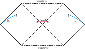
(a)

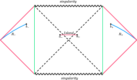
(b)

Figure 1: The schematic Penrose diagram of black holes (with the single horizon). The radiation regions are denoted by $R{\pm}$, and their boundaries are the cut-off surfaces. The coordinates of the radiation are $b_{\pm}=(\pm t_{b},b)$. The coordinates of the islands boundaries are $a_{\pm}=(\pm t_{a},a)$. On the left, this represents an asymptotically flat black hole. Hawking radiation can naturally diffuse to null infinity. On the right, it represents an asymptotically AdS black hole in thermal equilibrium with the bath (red region). We then impose the transport boundary condition on the black hole region (black region) island rule . In such way, Hawking radiation can also be collected by observers at space-like infinity.

$$\begin{split}\text{Right Wedge}:\ \ &U\equiv-e^{-\kappa u}=-e^{\kappa(t-r_{\star})};\qquad V\equiv+e^{+\kappa v}=+e^{+\kappa(t+r_{\star})},\\ \text{Left Wedge}:\ \ &U\equiv+e^{-\kappa u}=+e^{\kappa(t-r_{\star})};\qquad V\equiv-e^{+\kappa v}=-e^{+\kappa(t+r_{\star})},\end{split}$$ (5)

with the surface gravity $\kappa$:

$$\kappa\equiv 2\pi T_{H}=\frac{1}{2}f^{\prime}(r_{h}),$$ (6)

where $T_{H}$ is the Hawking temperature and $\prime$ represents the derivative with respect to the radial coordinate $r$, and $r_{h}$ is denoted the radius of event horizons. Here we set $f(r_{h})=0$. The tortoise coordinates is defined by

$$r_{\star}(r)=\int^{r}\frac{1}{f(r)}d\tilde{r}.$$ (7)

After the Kruskal transformation, the metric (4) can be recast as:

$$ds^{2}=-\Omega^{2}(r)dUdV+R(r)h_{ij}dx^{i}dx^{j},$$ (8)

with the conformal factor:

$$\Omega_{\text{BH}}(r)=\frac{\sqrt{f(r)}}{\kappa e^{\kappa r_{\star}(r)}},$$ (9a)

$$\Omega_{\text{bath}}(r)=\frac{1}{\kappa e^{\kappa r}}.$$ (9b)

2.1 No islands at early times

At first, we consider the issue from the perspective of an observer at the infinity, which means that $b-r_{h}\gg r_{h}$. In this case, we can only consider two-dimensional (2D) massless scalar field and assume the “s-wave approximation” is hold. In addition, we assume that the black holes is a pure state at initial time.

In the construction of the no-island, only radiation remains. We can only consider the complementary region of radiation based on the complementary of von Neumann entropy. As a consequence (see Appendix A):

$$\begin{split}S_{\text{Rad}}&=S(R)=\frac{c}{6}\log\Big{[}d^{2}(b_{-},b_{+})\Omega(b_{-})\Omega(b_{+})\Big{]}\\ &=\left\{\begin{array}[]{lr}\frac{c}{6}\log\bigg{(}\frac{4f(b)}{\kappa^{2}}\cosh^{2}(\kappa t_{b})\bigg{)},\qquad\text{for asymptotically flat black holes}&\\ \frac{c}{6}\log\bigg{(}\frac{4}{\kappa^{2}}\cosh^{2}(\kappa t_{b})\bigg{)},\qquad\ \ \ \text{for asymptotically AdS black holes}&\end{array}\right.\end{split}$$ (10)

where $c$ represents the central charge. In the limit of late times and large distances, we can take the approximation: $\cosh(\kappa t_{b})\simeq\frac{1}{2}e^{\kappa t_{b}}$. Then the above equation is equal to:

$$S_{\text{Rad}}(\text{without island})\simeq\frac{c}{3}\kappa t_{b}.$$ (11)

Apparently, without island construction, the entanglement entropy of radiation grows linearly with time at late times, which leads to the information loss and consistent with Hawking’s view. In addition, the result (11) does not depend on the geometry $f(r)$, which implies that the information paradox is always exists.

Next, we turn to the construction with an island to obtain the Page curve. Similarly, referring to the Penrose diagram in Figure.1, we see the entire Cauchy slice is divided into three intervals. For the disconnected union interval $R\cup I$, the expression of the entanglement entropy is converted from (10) (only valid for a single interval) to the following form ee formula1 ; ee formula2 :

$$\begin{split}S_{\text{bulk}}(R\cup I)&=\frac{c}{3}\log\bigg{(}\frac{d(a_{+},a_{-})d(b_{+},b_{-})d(a_{+},b_{+})d(a_{-},b_{-})}{d(a_{+},b_{-})d(a_{-},b_{+})}\bigg{)}\\ &=\frac{c}{6}\log\Big{[}16\Omega^{2}(a)\Omega^{2}(b)e^{2\kappa(r_{\star}(a)+r_{\star}(b))}\cosh^{2}(\kappa t_{a})\cosh^{2}(\kappa t_{b})\Big{]}\\ &+\frac{c}{3}\log\bigg{[}\frac{\cosh[\kappa(r_{\star}(a)-r_{\star}(b))]-\cosh[\kappa(t_{a}-t_{b})]}{\cosh[\kappa(r_{\star}(a)-r_{\star}(b))]+\cosh[\kappa(t_{a}+t_{b})]}\bigg{]},\end{split}$$ (12)

where

$$\Omega^{2}(a)\Omega^{2}(b)=\Omega^{2}_{\text{BH}}(a)\Omega^{2}_{\text{BH}}(b)=\frac{f(a)f(b)}{\kappa^{4}e^{2\kappa(r_{\star}(a)+r_{\star}(b))}},\ \ \ \text{for asymptotically flat cases}$$ (13a)

$$\Omega^{2}(a)\Omega^{2}(b)=\Omega^{2}_{\text{BH}}(a)\Omega^{2}_{\text{bath}}(b)=\frac{f(a)}{\kappa^{4}e^{2\kappa(r_{\star}(a)+b)}}.\qquad\text{for asymptotically AdS cases}$$ (13b)

Accordingly, the generalized entropy read as:

$$\begin{split}S_{\text{gen}}&=\frac{A(a)}{2G_{N}}+\frac{c}{6}\log\bigg{[}\frac{16f(a)f(b)}{\kappa^{4}}\cosh^{2}(\kappa t_{a})\cosh^{2}(\kappa t_{b})\bigg{]}\\ &+\frac{c}{3}\log\bigg{[}\frac{\cosh[\kappa(r_{\star}(a)-r_{\star}(b))]-\cosh[\kappa(t_{a}-t_{b})]}{\cosh[\kappa(r_{\star}(a)-r_{\star}(b))]+\cosh[\kappa(t_{a}+t_{b})]}\bigg{]},\end{split}$$ (14)

where $A(a)$ is the area of island, which is a positive constant and determined by the function $R(r)$ (4).

At very early times, we assume that $t_{a}\simeq t_{b}\simeq 0\ll\kappa b$. Then the generalized entropy becomes:

$$S_{\text{gen}}^{(\text{early})}\simeq\frac{A(a)}{2G_{N}}+\frac{c}{6}\log\bigg{[}\frac{16f(a)f(b)}{\kappa^{4}}\cosh^{2}(\kappa t_{a})\cosh^{2}(\kappa t_{b})\bigg{]}.$$ (15)

In order to obtain the QES, we extremize the above expression with respect to $a$ and $t_{a}$:

$$\frac{\partial S_{\text{gen}}^{(\text{early})}}{\partial t_{a}}=\frac{c\kappa}{3}\tanh(\kappa t_{a})=0.$$ (16)

The only solution is $t_{a}=0$, so the approximation is right. Then the location of QES can be obtained by the following equation:

$$\frac{\partial S_{\text{gen}}^{\text{(early)}}}{\partial a}=\frac{A^{\prime}(a)}{2G_{N}}+\frac{c}{6}\frac{f^{\prime}(a)}{f(a)}=0.$$ (17)

We can rewrite this expression to obtain the constraint equation that is satisfied if the island appears at early times:

$$-\frac{3A^{\prime}(a)f(a)}{f^{\prime}(a)}=cG_{N}\ll 1.$$ (18)

Here, we assume that the central charge is relatively small: $0<cG_{N}\ll 1$. This is because the area term $A^{\prime}(a)$ is finite. The only possible solution to the above equation is:

$$f^{\prime}(a)<0,\qquad a\gtrsim 0.$$ (19)

However, the size of island is now less than the Planck length $\ell_{p}(\sim\sqrt{G_{N}}$ for 4D case). One should discard this solution, which is consistent with our expectation. Namely, we can infer that islands absent at early times, which does not depend on the metric (4).

2.2 Constraints on the background geometry at late times

By contrast, at large distances and late times, the left wedge and right wedges are significantly separated. To simplify this, we can perform the following approximation high4 :

$$d(a_{+},a_{-})\simeq d(b_{+},b_{-})\simeq d(a_{+},b_{-})\simeq d(a_{-},b_{+})\gg d(a_{+},b_{+})\simeq d(a_{-},b_{-}).$$ (20)

Then, the entanglement entropy at late times is simplified as:

$$\begin{split}S_{\text{gen}}^{(\text{late})}&\simeq\frac{A(a)}{2G_{N}}+\frac{c}{3}\log[d(a_{+},b_{+})d(a_{-},b_{-})]\\ &=\frac{A(a)}{2G_{N}}+\frac{c}{6}\log\bigg{[}\frac{4f(a)f(b)}{\kappa^{4}}\bigg{(}\cosh(\kappa(r_{\star}(a)-r_{\star}(b)))-\cosh(\kappa(t_{a}-t_{b}))\bigg{)}^{2}\bigg{]}.\end{split}$$ (21)

In same way, we extremize it with respect to time $t_{a}$ firstly,

$$\frac{\partial S_{\text{gen}}^{\text{(late)}}}{\partial t_{a}}=-\frac{c}{3}\frac{\kappa\sinh[\kappa(t_{a}-t_{b})]}{\cosh[\kappa(r_{\star}(a)-r_{\star}(b))]-\cosh[\kappa(t_{a}-t_{b})]}=0.$$ (22)

The only solution is to set $t_{a}$ equal to $t_{b}$, and then substitute this relation into the original expression with respect to $a$,

$$\frac{\partial S_{\text{gen}}^{(\text{late})}}{\partial a}=\frac{A^{\prime}(a)}{2G_{N}}+\frac{c}{6}\bigg{[}\frac{f^{\prime}(a)}{f(a)}+\frac{2\kappa}{f(a)}\coth\Big{[}\frac{\kappa}{2}(r_{\star}(a)-r_{\star}(b))\Big{]}\bigg{]}=0,$$ (23)

where we have used $r_{\star}^{\prime}(a)=\frac{1}{f(a)}$. Following (18), we rewrite this expression as:

$$\frac{3A^{\prime}(a)f(a)}{2\kappa\frac{e^{\kappa x}+1}{e^{\kappa x}-1}-f^{\prime}(a)}=cG_{N}\ll 1,$$ (24)

where $x\equiv r_{\star}(b)-r_{\star}(a)\gg r_{h}$. Now we make the near horizon limit: $a\simeq r_{h}$ and obtain:

$$f(r)\simeq f^{\prime}(r_{h})(r-r_{h})+{\cal O}[(r-r_{h})^{2}],$$ (25a)

$$r_{\star}(r)=\int^{r}\frac{d\tilde{r}}{f(r)}\simeq\frac{1}{2\kappa}\log\bigg{|}\frac{r-r_{h}}{r_{h}}\bigg{|}.$$ (25b)

Substituting these equations into (24), yields the following constraint equation:

$$0<y(r)=\frac{3A^{\prime}(a)f^{\prime}(r_{h})(a-r_{h})^{2}}{f(a)\frac{e^{\kappa x}+1}{e^{\kappa x}-1}-(a-r_{h})f^{\prime}(a)}\simeq\frac{3A^{\prime}(a)f^{\prime}(r_{h})(a-r_{h})^{2}}{f^{\prime}(a)\frac{e^{\kappa x}+1}{e^{\kappa x}-1}-f^{\prime\prime}(a)}=cG_{N}\ll 1.$$ (26)

Firstly, we find that there is a solution to this equation in almost all cases, with the exception of the extremal case (see Appendix B). Additionally, it should be note that the island is consistently located outside of the event horizon:

$$a=r_{h}+\frac{cG_{N}}{6A^{\prime}(r_{h})}e^{\kappa r_{\star}(b)}+\frac{c^{2}G_{N}^{2}}{72A^{\prime 2}(r_{h})r_{h}}+{\cal O}[(cG_{N})^{3}].$$ (27)

Therefore, according to this location, we can obtain the entanglement entropy of radiation at late times:

$$\begin{split}S_{\text{Rad}}&=\frac{A(r_{h})}{2G_{N}}+{\cal O}(G_{N})\\ &\simeq 2S_{\text{BH}}.\end{split}$$ (28)

It is what we expect. Recall the result without island (11), the Page time is determined by

$$t_{\text{Page}}=\frac{6S_{\text{BH}}}{c\kappa}=\frac{3S_{\text{BH}}}{c\pi T_{H}}.$$ (29)

Besides, we can also calculate the scrambling time as a by-product. Drawing from the insights of the Hayden-Preskill thought experiment HP , it is posited that an external observer, situated asymptotically relative to the black hole, must patiently await the elapsed duration known as the "scrambling time" before information initially engulfed by the black hole can be retrieved through analyzing the emitted Hawking radiation. In the language of the entanglement wedge reconstruction, the scrambling time corresponds to the time when the information reaches the boundary of island ($r=a$) from the cut-off surface ($r=b$) entanglement wedge :

$$\begin{split}t_{\text{scr}}&\equiv\text{Min}[v(t_{b},b)-v(t_{a},a)]=r_{\star}(b)-r_{\star}(a)\\ &\simeq r_{\star}(b)-\frac{1}{2\kappa}\log\frac{a-r_{h}}{r_{h}}\simeq\frac{1}{2\kappa}\log\frac{A^{\prime}(r_{h})r_{h}}{cG_{N}}\\ &\simeq\frac{1}{2\pi T_{H}}\log S_{\text{BH}},\end{split}$$ (30)

where $t_{a},t_{b}$ is the time of sending and receiving information, respectively. In the penultimate line, we employed the approximation delineated in equation (25b) to facilitate our calculations. Concludingly, we adopted the established outcome for the four-dimensional scenario, aligning seamlessly with the findings reported in the seminal Hayden-Preskill thought experiment scrambling ; acoustic , thus ensuring theoretical consistency.

Above all, we protects the unitary by the island formula. In particular, by combining the discussion above with the expression (26), we also obtain a sufficient but not necessary condition for deriving the Page curve:

$$f^{\prime\prime}(r_{h}+{\cal O}(G_{N}))<0,$$ (31)

Specifically, the radial coordinate $r$ is confined to a region situated just outside the event horizon, adhering to the condition $r\gtrsim r_{h}$, reflecting our focus on the immediate vicinity of the horizon through implementation of the near-horizon approximation. Since we make the near horizon limit. In other words, if the above constraint is true, the equation (26) must have a solution, and then there is an island, which makes the entanglement entropy satisfy the Page curve. We present the results of calculations for some typical black holes in Appendix C. The impact of the condition on the result will be discussed in detail in the following section.

3 Island and Quantum Focusing Conjecture

Up to the present, we calculate the Page curve using the island formula (1). Combing the results of the previous section, we obtain the behavior of entanglement entropy in the entire process of black hole evaporation is

$$S_{\text{Rad}}=\text{Min}\Bigg{[}\frac{2\pi c}{3}T_{H}t,2S_{\text{BH}}\Bigg{]}.$$ (32)

In particular, we find that if the constraint condition (26) is satisfied, the Page curve must be reproduced, and there must exist an island outside the event horizon (27). This conclusion is universal and not depend on the explicit form of the metric (4). In this sense, we provide the constraint conditions of spacetime when Page curve is established.

Now in this section, we further prove the correctness of the constraint from the perspective of QFC. The classical focusing theorem asserts that the expansion $\theta$ of the congruence of null geodesic never increases:

$$\frac{d\theta}{d\lambda}\leq 0,$$ (33)

where $\lambda$ is the affine parameter. An important application of this theorem is to prove the second law of black holes. For a black hole with area $A$ and entropy $S_{\text{BH}}$($=\frac{A}{4G_{N}}$), the expansion $\theta$ is defined by:

$$\theta=\frac{1}{A}\frac{dA}{d\lambda}.$$ (34)

Then one can infer to the second law: $dS_{\text{BH}}\geq 0$.

However, once quantum effects are considered, i.e., the black hole emits Hawking radiation. The second law is violated. For the sake of rationality, this law should be upgraded to the generalized second law. Accordingly, the black hole entropy should be replaced by the generalized entropy: $dS_{\text{gen}}\geq 0$. Therefore, the classical focusing theorem is also being extended to the QFC qfc1 ; qfc2 , in which the quantum expansion is given by replacing the area in the classical expansion with the generalized entropy (21):

$$\frac{d\Theta}{d\lambda}\leq 0,$$ (35)

where $\Theta$ is the quantum expansion, which can be expressed in terms of the generalized entropy:

$$\Theta=\frac{1}{A}\frac{d}{d\lambda}S_{\text{gen}}.$$ (36)

Now, we investigate the QFC for the construction with an island. For the entanglement entropy at late times (21), the quantum expansion is written as:

$$\begin{split}\Theta&=\frac{1}{A}\frac{d}{d\lambda}S_{\text{gen}}\\ &=\frac{1}{A}\frac{dv_{b}}{d\lambda}\bigg{[}\frac{\partial S_{\text{gen}}}{\partial v_{b}}+\frac{dv_{a}}{dv_{b}}\frac{\partial S_{\text{gen}}}{\partial v_{a}}+\frac{du_{a}}{dv_{b}}\frac{\partial S_{\text{gen}}}{\partial u_{a}}\bigg{]}.\end{split}$$ (37)

Here we introduce the affine parameter qfc2 :

$$\lambda\equiv-\frac{\partial r(u,v)}{\partial u}dv,$$ (38)

for simplicity. Due to the fact that QES makes the entanglement entropy to extremized, which means that:

$$\frac{\partial S_{\text{gen}}}{\partial u_{a}}=\frac{\partial S_{\text{gen}}}{\partial v_{a}}=0.$$ (39)

Then we have

$$\begin{split}\Theta&=\frac{1}{A}\frac{dv_{b}}{d\lambda}\frac{\partial S_{\text{gen}}}{\partial v_{b}}=\frac{\partial S_{\text{gen}}}{\partial t_{b}}+f(b)\frac{\partial S_{\text{gen}}}{\partial b}\\ &=\frac{f(b)A^{\prime}(b)}{2G_{N}}-\frac{c\kappa}{3}\coth\bigg{[}\frac{\kappa}{2}((t_{a}-t_{b})+(r_{\star}(a)-r_{\star}(b)))\bigg{]}+\frac{c}{6}f^{\prime}(b)>0.\end{split}$$ (40)

Therefore, the entanglement entropy is always increasing with the null time $v_{b}$ and the quantum expansion is positive. Moreover, following the QFC, we obtain the derivative of the quantum expansion as:

$$\begin{split}\frac{d\Theta}{d\lambda}&=\frac{d}{d\lambda}\bigg{(}\frac{1}{A}\frac{dS_{\text{gen}}}{d\lambda}\bigg{)}\\ &=\frac{1}{d\lambda}\bigg{(}\frac{1}{A}\frac{dv_{b}}{d\lambda}\frac{\partial S_{\text{gen}}}{\partial v_{b}}\bigg{)}=\frac{1}{f(b)}\frac{d}{dv_{b}}X\\ &=-\frac{[A^{\prime}(b)]^{2}-A(b)A^{\prime\prime}(b)}{2G_{N}A^{2}(b)}-\frac{c}{6A^{2}(b)f^{2}(b)}(Y+Z),\end{split}$$ (41)

where

$$X =\frac{A^{\prime}(b)}{A(b)G_{N}}-\frac{c\kappa}{3A(b)f(b)}\coth\bigg{[}\frac{\kappa}{2}((t_{a}-t_{b})+(r_{\star}(a)-r_{\star}(b)))\bigg{]}+\frac{c}{6A(b)}\frac{f^{\prime}(b)}{f(b)},$$ (42a)

$$Y =-f(b)A^{\prime}(b)\bigg{(}2\kappa\coth\Big{[}\frac{\kappa}{2}((t_{a}-t_{b})+(r_{\star}(a)-r_{\star}(b)))\Big{]}-f^{\prime}(b)\bigg{)}>0,$$ (42b)

$$Z =A(b)\bigg{[}\kappa^{2}\text{csch}^{2}\Big{[}\frac{\kappa}{2}((t_{a}-t_{b})+(r_{\star}(a)-r_{\star}(b)))\Big{]}-2\kappa f^{\prime}(b)\times$$

$$\coth\Big{[}\frac{\kappa}{2}((t_{a}-t_{b})+(r_{\star}(a)-r_{\star}(b)))\Big{]}+(f^{\prime}(b))^{2}-f(b)f^{\prime\prime}(b)\bigg{]}.$$ (42c)

In above calculations, the QES condition (39) is used to be simplified. The first term is related to the area, which is always negative. Therefore, one can obviously see that if the QFC is hold, the only requirement is that $Z>0$. Further, since the first three terms of $Z$ are all positive, the we can find that as long as

$$f^{\prime\prime}(r>r_{h})<0,$$ (43)

where the radial coordinate $r$ can extended near the cutoff surface $r\sim b\gg r_{h}$. Then, there must be $\frac{d\Theta}{d\lambda}<0$, i.e. the QFC is satisfied.

In summary, we verify our previous conclusions from the perspective of QFC. The derived from QFC result (43) contain the previous result from island paradigm (31). Namely, the applicability of QFC is wider. Therefore, we can conclude that: A sufficient condition for a Page curve for general spacetime (4) to exist is the second derivative of the blacken function is negative in the near horizon region. We stress that this conclusion is only valid at the semi-classical level, where the back-reaction of black holes on spacetime can be ignored. Now we display some physical meaning of the result. When the “s-wave approximation” is allowed, we can only focus on the radial part of the metric (4) and ignore the angular momentum. For the metric (4), it can be reduced to:

$$ds^{2}=-f(r)dt^{2}+f(r)dr^{2}.$$ (44)

The second derivative of blacken function $f(r)$ is associated to the Ricci scalar curvature $R$, and can be positive or negative:

$$R=-f^{\prime\prime}(r).$$ (45)

Combine with the result (31), we can summarize that for the black hole spacetime with a positive Ricci scalar curvature, there always exists islands outside event horizons and Page curves can be derived. Moreover, the QFC is always satisfied in such cases. In brief, we verify the rationality of the result (31) again through the QFC.

4 Discussion and Conclusion

In conclusion, our study significantly contributes to the comprehension of black hole evaporation dynamics and the resolution of the information paradox, leveraging the insights from the Page curve and island paradigm. By examining diverse static black hole metrics within asymptotically flat or (anti-)de Sitter spacetimes, we revealed a pivotal geometric requirement: A metric with a negative second derivative near the horizon, $f^{\prime\prime}(r)<0$, in proximity to the event horizon where $r\sim r_{h}+{\cal O}(G_{N})$. which is fundamental for island formation and the consequent derivation of Page curves. This discovery affirms the universality of Page curves, transcending model-specific restrictions and reinforcing the compatibility of information conservation within the semi-classical gravity framework.

Our findings harmoniously intertwine quantum entanglement principles with the geometry of spacetime, with the QFC robustly supporting our conclusions. This integration bolsters our understanding of the intricate balance between information conservation, geometric configurations, and evaporative black hole dynamics, thus enriching the quantum gravity discourse.

We present a comprehensive method for calculating Page curves using a generalized metric (4), where the entanglement entropy of radiation follows (32). Notably, islands are positioned outside the event horizon (27), and we establish a sufficient condition (31) for island emergence. This methodology sets a benchmark for employing the island paradigm in Page curve computations.

Furthermore, we identify a pair of conditions ((31) and (43)) that jointly ensure the reproduction of unitary Page curves and adherence to QFC, thereby outlining a stringent criterion for island existence. Our analysis also implicates Ricci curvature, suggesting that spacetimes with positive Ricci curvature facilitate unitarity maintenance, whereas those with negative Ricci curvature necessitate deeper examination of the blacken function $f(r)$ and the fulfillment of the constraint (26).

Appendix A Entanglement Entropy in Curved Spacetime

In this appendix, we briefly give the expression of entanglement entropy in curved black hole background and discuss what should be pay attention to when using them.

Initially, different from the 2D simple case, the expression of entanglement entropy in the higher-dimensional scenario is complicated and has an area-like divergent. Namely, the entropy for matter fields has following expression:

$$S_{\text{bulk}}(R\cup I)=\frac{\text{Area}(\partial I)}{\epsilon^{2}}+S_{\text{bulk}}^{\text{finite}}(R\cup I),$$ (46)

where $\epsilon$ is the cutoff, which is dominates the area-like divergent term. Then we can absorb this term by renormalizing the Newton constant:

$$\frac{1}{4G_{N}^{(r)}}\equiv\frac{1}{4G_{N}}+\frac{1}{\epsilon^{2}}.$$ (47)

As consequent, we can replace the corresponding part of island formula (1) with $G_{N}^{(r)}$ and $S_{\text{bulk}}^{\text{finite}}(R\cup I)$, respectively, to yield a finite contribution of the entanglement entropy. Thus, the entanglement entropy in higher-dimensional spacetime is

$$S_{\text{Rad}}=\text{Min}\bigg{\{}\text{Ext}\bigg{[}\frac{\text{Area}(\partial I)}{4G_{N}^{(r)}}+S_{\text{bulk}}^{\text{(finite)}}(R\cup I)\bigg{]}\bigg{\}}.$$ (48)

Secondly, due to the s-wave approximation, the renormalized von Neumann entropy in vacuum CFT₂ in flat spacetime $ds^{2}=-dx^{+}dx^{-}$ (with the light cone coordinate $x^{\pm}=t\pm r$) is ee formula1 ; ee formula2

$$S_{\text{bulk}}(A\cup B)=\frac{c}{3}\log(d_{AB}),$$ (49)

with

$$d_{AB}\equiv\sqrt{[x^{+}(A)-x^{+}(B)][x^{-}(B)-x^{-}(A)]},$$ (50)

in the geodesic distance between points $A$ and $B$ in flat metric. In order to apply the formula (48) to the curved spacetime, we need to perform the Wely transformation into curved 2D metric $ds^{2}_{2D}=-\Omega^{2}(x^{+},x^{-})dx^{+}dx^{-}$ bulk entropy . After the Weyl transformation, we finally obtain the entanglement entropy in general 2D spacetime is 2d2 :

$$S_{\text{bulk}}(A\cup B)=\frac{c}{6}\log\bigg{[}d^{2}(A,B)\Omega(A)\Omega(B)\bigg{]}\Bigg{|}_{t_{\pm}=0}.$$ (51)

Appendix B Derivation of the Location of Islands

In this appendix, we display the details of the expression (27). From the equation (26)

$$0<y(r)=\frac{3A^{\prime}(a)f^{\prime}(r_{h})(a-r_{h})^{2}}{f(a)\frac{e^{\kappa x}+1}{e^{\kappa x}-1}-(a-r_{h})f^{\prime}(a)}=cG_{N}\ll 1.$$ (52)

For this equation to have a solution, the denominator has to be greater than zero, since the numerator is positive, namely,

$$f(a)\cdot\frac{e^{\kappa x}+1}{e^{\kappa x}-1}-(a-r_{h})f^{\prime}(a)>0,$$ (53)

Then, using the approximation (25a), we obtain:

$$\Big{[}f^{\prime}(r_{h})\frac{e^{\kappa x}+1}{e^{\kappa x}-1}-f^{\prime\prime}(r_{h})(a-r_{h})\Big{]}(a-r_{h})>0.$$ (54)

Since the first derivative of $f(r)$ at the horizon is related to the surface gravity of black holes: $\kappa=\frac{f^{\prime}(r_{h})}{2}$. It must be non-negative. While the second derivative of $f(r)$ is associated to the Ricci scalar curvature $R$ (45), and can be positive or negative.

When the island is beyond the horizon, $a-r_{h}>0$, the condition (53) is reduced to:

$$\frac{f^{\prime}(r_{h})}{(a-r_{h})}\cdot\frac{e^{\kappa x}+1}{e^{\kappa x}-1}>f^{\prime\prime}(r_{h}),$$ (55)

at large distances, $b\gg r_{h}$, we have:

$$\begin{split}x=r_{\star}(b)-r_{\star}(a)&\simeq\frac{b-r_{h}}{a-r_{h}},\\ \frac{e^{\kappa x}+1}{e^{\kappa x}-1}&\simeq 1.\end{split}$$ (56)

Therefore, (55) is becomes to

$$\frac{f^{\prime}(r_{h})}{a-r_{h}}>f^{\prime\prime}(r_{h}).$$ (57)

The LHS of the equation is a large positive number with order ${\cal O}(G_{N}^{-1})$, and RHS is order ${\cal O}(G_{N})$ and finite. So the above conditions are always true except in the special case of $f^{\prime}(r_{h})=0$ (which corresponding to the extremal black hole).

The other case is that the island is inside the horizon, $a-r_{h}<0$. Similarly, we just need to flip the symbol:

$$\frac{f^{\prime}(r_{h})}{r_{h}-a}<f^{\prime\prime}(r_{h}).$$ (58)

Based on the previous discussion, we find that this inequality can not be reached except in the extremal case $(f^{\prime}(r_{h})=0$. Accordingly, the island must always outside the horizon. Substituting $a\sim r_{h}$ into (52):

$$\begin{split}y(r)&\simeq\frac{3A^{\prime}(a)f^{\prime}(r_{h})(a-r_{h})^{2}}{f^{\prime}(r_{h})(a-r_{h})\frac{e^{\kappa x}+1}{e^{\kappa x}-1}-(a-r_{h})f^{\prime}(r_{h})}\\ &\simeq\frac{6A^{\prime}(a)(a-r_{h})}{e^{\kappa r_{\star}(b)}-\sqrt{\frac{a-r_{h}}{r_{h}}}-1}=cG_{N}.\end{split}$$ (59)

One finally obtains the location of the island (27).

Appendix C Tabulation

In this appendix, we give some results for several black holes based on the result (31). One can refer to Table 1 below:

Black Hole	$f(r)$	Area	$f^{\prime\prime}(r)$	Location of Islands
CGHS	$1-e^{-2\lambda(r-r_{h})}$	$e^{2\lambda r}$	$-4\lambda^{2}$	$a\simeq r_{h}+\frac{cG_{N}}{12\lambda e^{2\lambda r_{h}}}e^{\lambda r_{\star}(b)}$
JT	$\frac{r^{2}-r_{h}^{2}}{\ell^{2}}$	$\frac{r}{\ell}$	$\frac{2}{\ell^{2}}$	$a\simeq r_{h}+\frac{cG_{N}\ell}{6}e^{\frac{r_{h}}{\ell^{2}}r_{\star}(b)}$
BTZ	$\frac{r^{2}-r_{h}^{2}}{\ell^{2}}$	$2\pi r$	$\frac{2}{\ell^{2}}$	$a\simeq r_{h}+\frac{cG_{N}}{12\pi}e^{\frac{r_{h}}{\ell^{2}}r_{\star}(b)}$
Sch.	$1-\frac{r_{h}}{r}$	$4\pi r^{2}$	$-\frac{2}{r_{h}^{2}}$	$a\simeq r_{h}+\frac{cG_{N}}{48\pi r_{h}}e^{\frac{r_{\star}(b)}{2r_{h}}}$
Sch. AdS	$1-\frac{r_{0}}{r}+\frac{r^{2}}{\ell^{2}}$	$4\pi r^{2}$	$\frac{2}{\ell^{2}}-\frac{r_{0}}{r_{h}^{3}}$	$a\simeq r_{h}+\frac{cG_{N}}{48\pi r_{h}}e^{\big{(}\frac{r_{h}}{\ell^{2}}+\frac{r_{0}}{2r_{h}^{2}}\big{)}r_{\star}(b)}$
Sch. dS	$\frac{(r-r_{h})(r-r_{U})(r_{C}-r)}{3r\ell^{2}}$	$4\pi r_{h}^{2}$	$\frac{2(r_{C}r_{U}-r_{h}^{2})}{3\ell^{2}r_{h}^{2}}$	$a\simeq r_{h}+\frac{cG_{N}e^{\frac{(r_{c}-r_{h})(r_{h}-r_{u})}{6r_{h}\ell^{2}}}}{48\pi r_{h}e^{-r_{\star}(b)}}$
RN	$\big{(}1-\frac{r_{h}}{r}\big{)}\big{(}1-\frac{r_{-}}{r}\big{)}$	$4\pi r^{2}$	$-\frac{2(r_{h}-2r_{-})}{r_{h}^{3}}$	$a\simeq r_{h}+\frac{cG_{N}}{48\pi r_{h}}e^{\frac{r_{h}-r_{-}}{2r_{h}^{2}}r_{\star}(b)}$
Higher -dimensional Sch.	$1-\big{(}\frac{r_{h}}{r}\big{)}^{d-3}$	$\Omega_{d-2}r^{d-2}$	$-\frac{6-5d+d^{2}}{r_{h}^{2}}$	$a\simeq r_{h}+\frac{cG_{N}e^{\frac{d-3}{2r_{h}}}r_{\star}(b)}{12\Omega_{d-2}r_{h}^{d-3}}$

.

Table 1: The location of islands in several black holes.

References

- (1) S. W. Hawking, “Particle Creation by Black Holes,” Commun. Math. Phys. 43, 199 (1975). Erratum;[Commun. Math. Phys. 46, 206 (1976)].
- (2) S. W. Hawking, “Breakdown of Predictability in Gravitational Collapse,” Phys. Rev. D 14, (1976) 2460-2473.
- (3) D. N. Page, “Information in black hole radiation,” Phys. Rev. Lett. 71, 3743-3746 (1993) arXiv:hep-th/9306083.
- (4) D. N. Page, “Time Dependence of Hawking Radiation Entropy,” JCAP 1309, 028 (2013) arXiv:1301.4995.
- (5) J. Maldacena, “The Large N limit of superconformal field theories and supergravity,” Int. J. Theor. Phys. 38, 1113-1133 (1999) arXiv:hep-th/9711200.
- (6) S. Ryu and T. Takayanagi, “Holographic derivation of entanglement entropy from AdS/CFT,” Phys. Rev. Lett. 96, 181602 (2006) arXiv:hep-th/0603001.
- (7) A. Lewkowycz and J. Maldacena, “Generalized gravitational entropy,” JHEP 08, 090 (2013) arXiv:1304.4926.
- (8) N. Engelhardt and A. Wall, “Quantum Extremal Surfaces: Holographic Entanglement Entropy beyond the Classical Regime,” JHEP 01, 073 (2015) arXiv:1408.3203.
- (9) A. Almheiri, N. Engelhardt, D. Marolf and H. Maxfield, “The entropy of bulk quantum fields and the entanglement wedge of an evaporating black hole,” JHEP 12, 063 (2019) arXiv:1905.08762.
- (10) A. Almheiri, R. Mahajan, J. Maldacena and Y. Zhao, “The Page curve of Hawking ridiation from semiclassical geometry,” JHEP 03, 149 (2020) arXiv:1908.10996.
- (11) G. Penington, “Entanglement Wedge Reconstruction and the Information Paradox,” JHEP 09 002 (2020) arXiv:1905.08255.
- (12) A. Almheiri, T. Hartman, J. Maldacena, E. Shaghoulian and A. Tajdini, “The entropy of Hawking radiation,” Rev. Mod. Phys. 93, 35002 (2021) arXiv:2006.06872.
- (13) G. Penington, S. Shenker, D. Stanford and Z. Yang, “Replica wormholes and the black hole interior,” arXiv:1911.11977.
- (14) A. Almheiri, T. Hartman, J. Maldacena, E. Shaghoulian and A. Tajdini, “Replica Wormholes and the Entropy of Hawking Radiation,” JHEP 05, 013 (2020) arXiv:1911.12333.
- (15) A. Almheiri, R. Mahajan and J. Maldacena, “Islands outside the horizon,” arXiv:1910.11077.
- (16) T. Hollowood and S. Kumar, “Islands and Page Curves for Evaporating Black Holes in JT Gravity,” arXiv:2004.14944.
- (17) K. Goto, T. Hartman and A. Tajdini, “Replica wormholes for an evaporating 2D black hole,” JHEP 04, 289 (2021) arXiv:2011.09043.
- (18) T. Anegawa and N. Iizuka, “Notes on islands in asymptotically flat 2d dilaton black holes,” JHEP 07, 036 (2020) arXiv:2004.01601.
- (19) F. Gautason, L. Schneiderbauer, W. Sybesma and L. Thorlacius, “Page Curve for an Evaporating Black Hole,” JHEP 05, 091 (2020) arXiv:2004.00598.
- (20) T. Hartman, E. Shaghoulian and A. Strominger, “Islands in Asymptotically Flat 2D Gravity,” JHEP 07, 022 (2020) arXiv:2004.13857.
- (21) X. Wang, R. Li and J. Wang, “Islands and Page curves for a family of exactly solvable evaporating black holes,” Phys. Rev. D 103, 126026 (2021) arXiv:2104.00224.
- (22) R. Li, X. Wang and J. Wang, “Island may not save the information paradox of Liouville black holes,” Phys. Rev. D 104, 106015 (2021) arXiv:2105.03271.
- (23) M. Yu and X. Ge, “Entanglement Islands in Generalized Two-dimensional Dilaton Black Holes,” Phys. Rev. D 107, 066020 (2023) arXiv:2208.01943.
- (24) C. Lu, M. Yu and X. Ge, “Page Curve and Phase Transition in deformed Jackiw-Teitelboim Gravity,” Eur. Phys. J. C 83, 215 (2023) arXiv:2210.14750.
- (25) J. F. Pedraze, A. Svesko, W. Sybesma and M. R. Visser, “Microcanonical Action and the Entropy of Hawking Radiation,” Phys. Rev. D 105, 126010 (2022) arXiv:2111.06912.
- (26) J. F. Pedraze, A. Svesko, W. Sybesma and M. R. Visser, “Semi-classical thermodynamics of quantum extremal surfaces in Jackiw-Teitelboim gravity,” JHEP 12, (2021) 134 arXiv:2107.10358.
- (27) A. Almheiri, R. Mahajan and J. E. Santos, “Entanglement islands in higher dimensions,” SciPost Phys. 9, no.1, 001 (2020) arXiv:1911.09666.
- (28) S. He, Y. Sun, L. Zhao and Y. X. Zhang, “The universality of islands outside the horizon,” JHEP 05 (2022) 047 arXiv:2110.07598.
- (29) M. Alishahiha, A. Astaneh and A. Naseh, “Island in the presence of higher derivative terms,” JHEP 02, 035 (2021) arXiv:2005.08715.
- (30) K. Hashimoto, N. Iizuka and Y. Matsuo, “Islands in Schwarzschild black holes,” JHEP 06, 085 (2020) arXiv:2004.05863.
- (31) Y. Matsuo, “Islands and stretched horizon,” JHEP 07, 051 (2021) arXiv:2011.08814.
- (32) H. Geng, A. Karch, C. Perez-Pardavila, S. Raju, L. Randall, M. Riojas and S. Shashi, “Inconsistency of islands in theories with long-range gravity,” JHEP 01, (2022) 182 arXiv:2107.03390.
- (33) H. Geng and A. Karch, “Massive islands,” JHEP 09, 121 (2020) arXiv:2006.02438.
- (34) C. Krishnan, “Critical islands,” JHEP 01, 179 (2021) arXiv:2007.06551.
- (35) C. Krishnan, V. Patil and J. Pereira, “Page Curve and the Information Paradox in Flat Space,” arXiv:2005.02993.
- (36) F. Omidi, “Entropy of Hawking Radiation for Two-Sided Hyperscaling Violating Black Branes,” JHEP 04, 022 (2022) arXiv:2112.05890.
- (37) C. F. Uhlemann, “Islands and Page curves in 4d from Type IIB,” JHEP 08, 104 (2021) arXiv:2105.00008.
- (38) C. F. Uhlemann, “Information transfer with a twist,” JHEP 01, 126 (2022) arXiv:2111.11443.
- (39) P. Hu, D. Li and R. Miao, “Island on codimension-two branes in AdS/dCFT,” JHEP 11, 008 (2022) arXiv:2208.11982.
- (40) G. Karananas, A. Kehagias and J. Taskas, “Islands in linear dilaton black holes,” JHEP 03, 253 (2021) arXiv:2101.00024.
- (41) Y. Lu and J. Lin, “Islands in Kaluza-Klein black holes,” Eur. Phys. J. C 82, 132 (2022) arXiv:2106.07845.
- (42) T. Li, J. Chu and Y. Zhou, “Reflected Entropy for an Evaporating Black Hole,” JHEP 11, 155 (2020) arXiv:2006.10846.
- (43) F. Deng, J. Chu and Y. Zhou, “Defect extremals surface as the holographic counterpart of Island formula,” JHEP 03, 008 (2021) arXiv:2012.07612.
- (44) J. Chu, F. Deng and Y. Zhou, “Page Curve from Defect Extremal Surface and Island in Higher Dimensions,” JHEP 10, 149 (2021) arXiv:2105.09106.
- (45) T. Li, M. Yuan and Y. Zhou, “Defect Extremal Surface for Reflected Entropy,” JHEP 01, 018 (2022) arXiv:2108.08544.
- (46) C. Chou, H. Lao and Y. Yang, “Page Curve of Effective Hawking Radiation,” Phys. Rev. D 106, 066008 (2022) arXiv:2111.14551.
- (47) M. Yu, C. Lu, X. Ge and S. Sin, “Island, Page Curve and Superradiance of Rotating BTZ Black Holes,” Phys. Rev. D 105, 066009 (2022) arXiv:2112.14361.
- (48) W. Gan, D. Du and F. Shu, “Island and Page curve for one-sided asymptotically flat black hole,” JHEP 07, 020 (2022) arXiv:2203.06310.
- (49) D. Du, W. Gan, F. Shu and J. Sun, “Unitary Constraints on Semiclassical Schwarzschild Black Holes in the Presence of Island,” Phys. Rev. D 107, 026005 (2023) arXiv:2206.10339.
- (50) H. Geng, A. Karch, C. Perez-Pardavila, S. Raju, L. Randall, M. Riojas and S. Shashi, “Information Transfer with a Gravitating Bath,” SciPost Phys. 10 (2021) 103 arXiv:2012.04671.
- (51) H. Geng, A. Karch, C. Perez-Pardavila, S. Raju, L. Randall, M. Riojas and S. Shashi, “Entanglement phase structure of a holographic BCFT in a black hole background,” JHEP 05, (2022) 153 arXiv:2112.09132.
- (52) H. Geng, S. Lust, R. K. Mishra and D. Wakeham, “Holographic BCFTs and Communicating Black Holes,” JHEP 08, (2021) 003 arXiv:2104.07039.
- (53) Y. Ling, Y. Liu and Z. Xian, “Island in charged black holes,” JHEP 03, 251 (2021) arXiv:2010.00037.
- (54) X. Wang, R. Li and J. Wang, “Islands and Page curves of Reissner-Nordstrm black holes,” JHEP 04, 103 (2021) arXiv:2101.06867.
- (55) W. Kim and M. Nam, “Entanglement entropy of asymptotically flat non-extremal and extremal black holes with an island,” Eur. Phys. J. C 81, 869 (2021) arXiv:2103.16163.
- (56) B. Ahn, S. Bak, H. Jeong, K. Y. Kim and Y. W. Sun, “Islands in charged linear dilaton black holes,” Phys. Rev. D 105, 046012 (2022) arXiv:2107.07444.
- (57) M. Yu and X. Ge, “Page Curves and Islands in Charged Dilaton Black Holes,” Eur. Phys. J. C 02, 82 (2022) arXiv:2107.03031.
- (58) G. Yadav, “Page Curves of Reissner-Nordstrm black hole in HD Gravity,” Eur. Phys. J. C 82, 904 (2022) arXiv:2204.11882.
- (59) J. Vuyst and T. Mertens, “Operational islands and black hole dissipation in JT gravity,” JHEP 01, (2023) 027 arXiv:2207.03351.
- (60) H. Geng, Y. Nomura and H. Sun, “An Information Paradox and Its Resolution in de Sitter Holography,” Phys. Rev. D 103, 126004 arXiv:2103.07477.
- (61) C. Chu and R. Miao, “Tunneling of Bell Particles, Page Curve and Black Hole Information,” arXiv:2209.03610.
- (62) B. Craps, J. Hernandez, M. Khramtsov and M. Knysh, “Delicate windows into evaporating black holes,” JHEP 02, 080 (2023) arXiv:2209.15477.
- (63) G. Yadav and N. Joshi, “Cosmological and black hole Islands in multi-event horizon spacetimes,” Phys. Rev. D 107, 026009 (2023) arXiv:2210.00331.
- (64) Y. Lu and J. Lin, “The Markov gap in the presence of islands”, JHEP 03, (2023) 043 arXiv:2211.06886.
- (65) D. Basu, Q. Wen and S. Zhou, “Entanglement Islands from Hilbert Space Reduction,” arXiv:2211.17004.
- (66) D. Basu, J. Lin, Y. Lu and Q. Wen, “Ownerless island and partial entanglement entropy in island phases,” arXiv:2305.04259.
- (67) M. Yu, X. Ge and C. Lu, “Page Curves for Accelerating Black Holes,” Eur. Phys. J. C 83, 1104 (2023) arXiv:2306.11407.
- (68) H. Geng, “Revisiting Recnet Progress in Karch-Randall Braneworld,” arXiv:2306.15671.
- (69) J. Chang, S. He, Y. Liu and L. Zhao, “Island formula in Planck brane,” arXiv:2308.03645.
- (70) Z. Li and Z. Hong, “Islands on codim-2 branes in Gauss-Bonnet Gravity,” arXiv:2308.15861.
- (71) S. Hirano, “Island Formula from Wald-like Entropy with Backreaction,” arXiv:2310.03416.
- (72) F. Deng, Z. Wang and Y. Zhou, “End of the World Brane metts ,” arXiv:2310.15031.
- (73) C. Tong, D. Du and J. Sun, “Island of Reissner-Nordstrm anti-de Sitter black holes in the large limit,” arXiv:2306.06682.
- (74) R. Bousso and G. Penington, “Islands Far Outside the Horizon,” arXiv:2312.03078.
- (75) H. Geng, “Graviton Mass and Entanglement Islands in Low Spacetime Dimensions,” arXiv:2312.13336.
- (76) A. Chandra, Z. Li and Q. Wen, “Entanglement islands and cutoff branes from path-integral optimization,” arXiv:2402.15836.
- (77) A. R. Chowdhury, A. Saha, and S. Gangopadhyay, “Mutual information of subsystems and the Page curve for the Schwarzschild-de Sitter black hole,” Phys. Rev. D 108, 026003 (2023) arXiv:2303.14062.
- (78) A. R. Chowdhury, A. Saha, and S. Gangopadhyay, “The role of mutual information in the Page curve,” Phys. Rev. D 106, 086019 (2022) arXiv:2207.13029
- (79) A. Saha, S. Gangopadhyay, and J. P. Saha, “Mutual information, islands in black holes and the Page curve,” Eur. Phys. J. C. 82, 476 (2022) arXiv:2109.02996.
- (80) D. Basu, H. Parihar, V. Raj, and G, Sengupta, “Defect extremal surfaces for entanglement negativity,” arXiv:2205.07905.
- (81) M. Afrasiar, D. Baasu, A. Chandra, V. Raj, and G, Sengupta, “Islands and dynamics at the interface,” arXiv:2306.12476.
- (82) D. Basu, H. Parihar, V. Raj, and G, Sengupta, “Reflected entropy in BCFTs on a black hole background,” arXiv:2311.17023.
- (83) S. Azarnia, R. Fareghbal, A. Naseh, and Zolfi, “Islands in Flat-Space Cosmology,” Phys. Rev. D 104, 126017. arXiv:2109.04795.
- (84) H. Jeong, K. Kim, and Y. Sun, “Entanglement entropy analysis of dyonic black holes using doubly holographic theory,” arXiv:2305.18122.
- (85) S. Lin, M. Yu, X. Ge, and L. Tian, “Entanglement Entropy, Phase Transition, and Island Rule for Reissner-Nordstrm-AdS Black Holes,” arXiv: 2405.06873.
- (86) ] O.J.C. Dias, P. Figueras, S. Minwalla, P. Mitra, R. Monteiro and J.E. Santos, “Hairy black holes and solitons in global AdS5”, JHEP 08, 117 (2012) arXiv:1112.4447.
- (87) D. Garfinkle, G. T. Horowitz, and A. Strominger, “Charged black holes in string theory,” Phys. Rev. D 43, 3140 (1991).
- (88) P. Calabrese and J. Cardy, “Entanglement entropy and quantum field theory,” J. Stat. Mech. 0406, P002 (2004) arXiv:hep-th/0405152.
- (89) H. Casini, C. D. Fosco and M. Huerta, “Entanglement and alpha entropies for a massive Dirac field in two dimensions,” J. Stat. Mech. 0507, P07007, 2005 arXiv:cond-mat/0505563.
- (90) P. Hayden and J. Preskill, “Black holes as mirrors: Quantum information in random subsystems,” JHEP 09, 120 (2007) arXiv:0708.4025.
- (91) Y. Sekino and L. Susskind, “Fast Scramblers,” JHEP 10, 065 (2008) arXiv:0808.2096.
- (92) Q. Wang, M. Yu and X. Ge, “Scrambling time for analogue black holes embedded in AdS space,” Eur. Phys. J. C 82, 468 (2022) arXiv:2203.07914.
- (93) R. Bousso, Z. Fisher, S. Leichenauer and A. C. Wall, “Quantum focusing conjecture,” Phys. Rev. D 93 (2016) 064044 arXiv:1506.02669.
- (94) Y. Matsuo, “Quantum focusing conjecture and the Page curve,” JHEP 12, 050 (2023) arXiv:2308.05009.
- (95) J. Maldacena and L. Susskind, “Cool horizons for entangled black holes,” Fortsch. Phys. 61, 781-811 (2013) arXiv:1306.0533.