A Dynamical Simulation Model of a Cement Clinker Rotary Kiln

Abstract

This study provides a systematic description and results of a dynamical simulation model of a rotary kiln for clinker, based on first engineering principles. The model is built upon thermophysical, chemical, and transportation models for both the formation of clinker phases and fuel combustion in the kiln. The model is presented as a 1D model with counter-flow between gas and clinker phases and is demonstrated by a simulation using industrially relevant input. An advantage of the proposed model is that it provides the evolution of the individual compounds for both the fuel and clinker. As such, the model comprises a stepping stone for evaluating the development of process control systems for existing cement plants.

I Introduction

In this paper, a differential-algebraic model of the dynamics of a rotary kiln is proposed, with the intention of modeling the formation of clinker and combustion. The modeling approach is primarily based on first engineering principles, to provide an intuitive understanding of the processes included.

I-A Background and motivation

The cement industry accounts for 8% of the world’s CO_2 emissions [1]. A main contributor to these CO_2 emissions and energy consumption is the production of clinker; a main component in the cement. For example, Ordinary Portland Cement comprises ca. 90% clinker, with the remainder being gypsum and other mineral additions (e.g. limestone). The strength of cement depends on its composition, especially the amount of C_3S, and thus depends on the composition of the clinker, the clinker quality, to provide enough strength. In addition, considerable fluctuations in the clinker composition can limit the utilization of supplementary cementitious materials (SCMs) - because a greater percentage of clinker is likely required to cover for the resulting variability in cement strength. In view of that, reducing uncertainty and variations of the clinker quality is thus a must to enable a more sustainable and controlled cement production.

The uncertainty can be addressed by improving the quality predictions and the variation through control of the operation. The design of both approaches requires the availability of system responses, from either an actual system or a simulation model, to account for the dynamical transitions between operation states. Although a simulation model does not account for all process details, it enables cost-effective and faster testing without disrupting a production site.

The production of clinker comprises several process equipment: a pre-heating tower (with a set of cyclones), a calciner, a rotary kiln, and a cooler, see Fig. 1. As the formation of clinker takes place in the rotary kiln, this paper focuses on formulating a dynamical model for the rotary kiln.

Figure 1: Simplified Clinker Production Line: preheating Cyclones (P), Calciner (Ca), Rotary Kiln (K), and Cooler (Co)

I-B Research review

Several models have been proposed in the literature to describe the kiln. Most of these focuses on steady-state descriptions of the kiln [2]-[4], while few give a dynamic description [5]-[8].

Spang’s dynamic model [5] includes a description of the bed chemistry and temperature energy balances. In Sun’s model [6], the temperature is also described, while the mass balance only considers the overall bulk matter. Similarly, in Liu’s model, [7] the bulk bed/gas is considered with added momentum balance; while Ginsberg [8] assumes a steady-state gas balance in its dynamic description.

Mastorakos [4] presented a detailed steady-state model with a 3D temperature energy balance, a 1D mass balance, and constant velocities. The combustion and gas parts were only mentioned briefly in words. Further, the steady-state model of Hanein [3] only contains the energy balance, while Mujumdar’s model [2] outlines the temperature energy balances and solid mass balance accounting for particle size, though it does not consider the gas mass balance nor the fuel part.

I-C Contribution

In none of the reported models, the fuel chemistry is accounted for, and only few consider the gas mass dynamics and velocity changes. Thus, it is not trivial to potentially include modern considerations, e.g. the effects of ash content from alternative fuels or gas reactions giving non-CO2 emissions e.g. NO_x.

To address these limitations, this paper aims to present a dynamic kiln model where: 1) the description preserves the physical overview and understanding of the system; 2) it is easy to modify, for the inclusion of new scenarios or descriptions; and 3) the dynamics of the individual compounds is modeled, e.g. CO2 content.

The presented model covers the main dynamics of the kiln with the following simplifications and assumptions: 1) it is a 1D-model (axial); 2) the heat loss to the environment is negligible; and 3) only the primary clinker- and combustion reactions are included.

The standard cement chemist notation will be used for the following compounds, i.e.: (CaO)_2SiO_2 as C_2S, (CaO)_3SiO_2 as C_3S, (CaO)_3Al_2O_3 as C_3A and (CaO)_4(Al_2O_3)(Fe_2O_3) as C_4AF, where C, A, S and F refers to CaO, Al_2O_3, SiO_2 and Fe_2O_3, respectively. Finally $\partial_{x}$ will note the differential $\partialderivative{x}$

II Model Layout

The kiln model is formulated as a Differential-Algebraic system, with dynamic descriptions of the concentrations $C$ and internal energy densities $\hat{U}$, and algebraic relations for the temperatures $T$, pressures $P$, and fill angle $\theta$:

$$\partial_{t}x =f(x,y),\quad x=[C;\hat{U}]$$ (1a)

$$0 =g(x,y),\quad y=[T;P;\theta].$$ (1b)

For clarity, the different aspects of the kiln model are discussed separately in order of computation: A) Thermophysical model, B) Geometry, C) Transportation, D) Stoichiometry & Kinetics, E) Mass balances, F) Energy balances, and G) Algebraic relations.

III Kiln Model

A rotary kiln is a rotating cylinder of length $L$ and inner radius $r_{c}$ with an inclination $\psi$, Fig. 2 illustrates the kiln’s cross and axial profiles. We use a finite-volume approach to describe the kiln in $n_{v}$ segments of length $\Delta z=L/n_{v}$ and volumes $V_{\Delta}=\pi r_{c}^{2}\Delta z$. The model segment consists of 3 phases; wall (_w), solids (_s), and gasses (_g). The concentrations are of the individual compounds of each phase.

III-A Thermophysical model

If we define concentration $C$ as mole per total segment volume $V_{\Delta}$ and assume gasses are ideal, then the enthalpy and volumes for the solid and gas part can be defined as functions $H$ and $V$, linear w.r.t. the moles, e.g.:

$$H(T,P,n) =\sum_{i}(\Delta H_{\mathrm{f},i}^{\circ}+\int^{T}_{T_{0}}c_{m,i}(\tau)d\tau)n_{i}$$ (2)

$$V_{s}(T,P,n) =\sum_{i}\frac{M_{i}}{\rho_{i}}n_{i},\quad V_{g}(T,P,n)=\frac{RT}{P}\sum_{i}n_{i}.$$ (3)

The enthalpy- and volume densities are obtained by the H and V functions, by applying the concentrations instead:

$$\hat{H}_{s} =H(T_{s},P,C_{s}),\quad \hat{V}_{s} =V(T_{s},P,C_{s})$$ (4)

$$\hat{H}_{g} =H(T_{g},P,C_{g}),\quad \hat{V}_{g} =V(T_{g},P,C_{g}).$$ (5)

with the solid- and gas volumes obtained by their densities:

$$V_{g}=\hat{V}_{g}V_{\Delta},\quad V_{s}=\hat{V}_{s}V_{\Delta}.$$ (6)

The energy densities of each phase are then described by:

$$\hat{U}_{g}=\hat{H}_{g}-P\hat{V}_{g},\quad\hat{U}_{s}=\hat{H}_{s},\quad\hat{U}_{w}=H(T_{w},P,\rho_{w}).$$ (7)

III-B Geometric relationships

(a) Cross section.

(b) Axial profile with segment notation for the $k$-th volume.

Figure 2: Kiln profiles

The gas and solid volumes across the kiln define the geometric aspect of each segment. The solid volume $V_{s}$ gives the bed height $h$, through the cross-section area:

$$V_{s}(z_{k})=\int_{z_{k-\frac{1}{2}}}^{z_{k+\frac{1}{2}}}A_{s}(z)dz.$$ (8)

As the cross section $A_{s}$ of the solids forms a circle segment [9], see Fig. 2(a), the cross-area defines the bed height $h$, the surface chord $L_{c}$, the fill angle $\theta$, and the bed slope angle $\phi$:

$$A_{s}(z) =\frac{r_{c}^{2}}{2}(\theta(z)-\text{sin}(\theta(z)))$$ (9)

$$L_{c}(z) =2r_{c}\text{sin}(\frac{\theta(z)}{2}),\quad h(z)=r_{c}(1-\text{cos}(\frac{\theta(z)}{2}))$$ (10)

$$\phi(z) =\text{atan}\bigg{(}-\partialderivative{h(z)}{z}\bigg{)}.$$ (11)

The surface areas between the wall, gas, and solid along the segment, and the gas cross area $A_{g}$ are given by:

$$A_{g}(z) =\pi r_{c}^{2}-A_{s}(z)$$ (12)

$$A_{gs}(z_{k}) =\int_{z_{k-\frac{1}{2}}}^{z_{k+\frac{1}{2}}}L_{c}(z)dz$$ (13)

$$A_{ws}(z_{k}) =\int_{z_{k-\frac{1}{2}}}^{z_{k+\frac{1}{2}}}r_{c}\theta(z)dz$$ (14)

$$A_{gw}(z_{k}) =2\pi r_{c}\Delta z-A_{ws}(z_{k})$$ (15)

where $A_{gs}$ is the gas-solid surface area, $A_{gw}$ is the gas-wall surface area, and $A_{ws}$ is the wall-solid surface area.

III-C Transportation

The transportation of matter and energy in the kiln depends on material flux, heat flux, heat convection, and heat radiation. The details on these aspects are described as follows.

III-C1 Material flux

The flux of each compound is defined independently for solid and gas given their opposite flow. It consists of an advection term and a diffusion term:

$$N_{i,s} =v_{s}C_{i,s}+J_{i,s},\quad J_{i,s} =-D_{i,s}\partial_{z}C_{i,s}$$ (16)

$$N_{i,g} =v_{g}C_{i,g}+J_{i,g},\quad J_{i,g} =-D_{i,g}\partial_{z}C_{i,g}$$ (17)

with the diffusion $J_{i}$ given by Fick’s law [10].

Velocities

The advection term depends on the concentration and the phases’ velocity. The velocity of the solid depends on the rotational velocity of the kiln $\omega$:

$$v_{s}(z)=\omega\frac{\psi+\phi(z)\text{cos}(\xi)}{\text{sin}(\xi)}\frac{\pi L_{c}(z)}{\text{asin}(\frac{L_{c}(z)}{2r_{c}})}$$ (18)

$v_{s}$ is the average velocity at the location, accounting for the cascading motion due to the rotation [11]. The repose angle $\xi$ is related to the rotational velocity by

$$\xi=a_{\omega}\omega+b_{\omega}$$ (19)

with the coefficients determined experimentally [12, 13].

Given that the gas velocity in a kiln is below 0.2 Mach speed [14], according to Howel & Weathers [15], the Darcy-Weisbach equation in (20) is valid to describe the gas velocity, despite the gas being compressible.

$$v_{g}^{2}=2\frac{|\Delta P|}{\Delta z}\frac{D_{H}}{f_{D}\rho_{g}},$$ (20)

Assuming turbulent flow, the Darcy friction factor $f_{D}$ is

$$f_{D}=\frac{0.316}{\sqrt[4]{Re}}=\frac{0.316\sqrt[4]{\mu_{g}}}{\sqrt[4]{\rho_{g}|v_{g}|D_{H}}},\ D_{H}=\frac{4V_{g}}{A_{gw}+A_{gs}}$$ (21)

where $D_{H}$ is the hydraulic diameter for a Non-uniform nor circular channel [16]. The gas velocity is then given by

$$v_{g}=\Big{(}\frac{2}{0.316}\sqrt[4]{\frac{D_{H}^{5}}{\mu_{g}\rho_{g}^{3}}}\frac{|\Delta P|}{\Delta z}\Big{)}^{\frac{4}{7}}\text{sgn}\Big{(}\frac{\Delta P}{\Delta z}\Big{)},$$ (22)

since negative pressure difference leads to a negative flow.

Diffusion

The diffusion of each phase is defined by the diffusion coefficients $D_{i,s}$ and $D_{i,g}$. According to Mujumdar [2], solid diffusion can be neglected since an industrial kiln has a Peclet number greater than $10^{4}$, $D_{s}=0$.

For diffusion within a gas mixture, the coefficient is given by (23-24) using Fuller’s model [17], where $x_{j}$ is the mole fraction, $V_{\sum}$ the diffusion volume, and $M$ the molar mass.

$$D_{i,g} =\bigg{(}\sum_{\begin{subarray}{c}j=1\\ j\neq i\end{subarray}}\frac{x_{j}}{c_{g}D_{ij}}\bigg{)}^{-1},\ x_{j}=\frac{C_{j,g}}{c_{g}},\ c_{g}=\sum_{j}C_{j,g}$$ (23)

$$D_{i,j} =\frac{0.00143T^{1.75}}{PM_{ij}^{\frac{1}{2}}[(V_{\sum})^{\frac{1}{3}}_{i}+(V_{\sum})^{\frac{1}{3}}_{j}]^{2}},\ M_{ij}=\frac{2}{\frac{1}{M_{i}}+\frac{1}{M_{j}}}$$ (24)

III-C2 Heat conduction

The heat flux of each phase is given by Fourier’s law [10]:

$$\tilde{Q}_{i}=-k_{i}\partial_{z}{T_{i}},\quad\text{for }i=\{s,g,w\}$$ (25)

with $k_{i}$ being the conductivity of phase i, e.g. $k_{s}$ for the solid mixture.

III-C3 Heat convection

The transfer of heat due to convection between the gas, solid, and wall is given by [2]:

$$Q_{gs}^{cv} =A_{gs}\beta_{gs}(T_{g}-T_{s})$$ (26)

$$Q_{gw}^{cv} =A_{gw}\beta_{gw}(T_{g}-T_{w})$$ (27)

$$Q_{ws}^{cv} =A_{ws}\beta_{gw}(T_{w}-T_{s})$$ (28)

where $A_{ij}$ is the in-between surface area, and $\beta_{ij}$ is the convection coefficient. The coefficients of the three phases are defined by Tscheng [18] as:

$$\beta_{gs}= \frac{k_{g}}{D_{e}}Nu_{gs},\ Nu_{gs}=0.46Re_{D}^{0.535}Re_{\omega}^{0.104}\eta^{-0.341}$$ (29)

$$\beta_{gw} =\frac{k_{g}}{D_{e}}Nu_{gw},\quad Nu_{gw}=1.54Re_{D}^{0.575}Re_{\omega}^{-0.292}$$ (30)

$$\beta_{ws} =11.6\frac{k_{s}}{l_{w}}(\frac{\omega r_{c}^{2}\theta}{\alpha_{B}})^{0.3},\ \alpha_{B}=\frac{k_{s}}{\rho_{s}C_{ps}},\ l_{w}=r_{c}\theta$$ (31)

where $k_{i}$ is the conductivity of phase i, $D_{e}$ the effective diameter, $\alpha_{B}$ the thermal diffusivity, and $l_{w}$ the contact perimeter between the solid and wall. $Re_{D}$ and $Re_{\omega}$ are Reynold’s numbers and $\eta$ is the solid fill fraction:

$$Re_{D} =\frac{\rho_{g}v_{g}D_{e}}{\mu_{g}},\quad Re_{\omega}=\frac{\rho_{g}\omega D_{e}^{2}}{\mu_{g}}$$ (32)

$$\eta =\frac{\theta-\text{sin}(\theta)}{2\pi}\quad D_{e}=2r_{c}\frac{\pi-\frac{\theta}{2}+\frac{\text{sin}(\theta)}{2}}{\pi-\frac{\theta}{2}+\text{sin}(\frac{\theta}{2})}$$ (33)

with $\mu_{g}$ being the viscosity of the gas mixture.

The densities $\rho$ and heat capacity $C_{ps}$ are given by:

$$\rho_{j}=\frac{\sum_{i}M_{i}C_{j,i}}{\hat{V}_{j}},\quad C_{ps}=\sum_{i}n_{i}c_{m,i}$$ (34)

with $M$ being the molar mass and $c_{m}$ the molar heat capacity.

Viscosity & conductivity

For a single gas, Sutherland’s formula for temperature-dependent viscosity read [19]:

$$\mu_{g,i}=\mu_{0}\bigg{(}\frac{T}{T_{0}}\bigg{)}^{\frac{3}{2}}\frac{T_{0}+S_{\mu}}{T+S_{\mu}},$$ (35)

where $S_{\mu}$ can be calibrated given two measures of viscosity.

The viscosity and conductivity of a mixed gas are given by the similar formulas of Wilke [20] and Wassiljewa [17]:

$$\mu_{g} =\sum_{i}\frac{x_{i}\mu_{g,i}}{\sum_{j}x_{j}\phi_{ij}},\quad k_{g}=\sum_{i}\frac{x_{i}k_{g,i}}{\sum_{j}x_{j}\phi_{ij}}$$ (36)

$$\phi_{ij} =\bigg{(}1+\sqrt{\frac{\mu_{g,i}}{\mu_{g,j}}}\sqrt[4]{\frac{M_{j}}{M_{i}}}\bigg{)}^{2}\bigg{(}2\sqrt{2}\sqrt{1+\frac{M_{i}}{M_{j}}}\bigg{)}^{-1}.$$ (37)

For the conductivity of mixed solids, we apply the formula for conductivity through layers [10] using volumetric ratios, assuming layers with length $\Delta z_{i}$ and constant cross area:

$$k_{s}=\frac{1}{\sum_{i}\frac{V_{s,i}}{V_{s}}\frac{1}{k_{s,i}}},\quad\frac{V_{s,i}}{V_{s}}=\frac{\Delta z_{i}}{\Delta z}.$$ (38)

III-C4 Heat Radiation

Assuming axial radiation is negligible, then the heat transfer due to radiation is given by [2]:

$$Q_{gs}^{rad} =\sigma A_{gs}(1+\epsilon_{s})\frac{\epsilon_{g}T^{4}_{g}-\alpha_{g}T^{4}_{s}}{2}$$ (39)

$$Q_{gw}^{rad} =\sigma A_{gw}(1+\epsilon_{w})\frac{\epsilon_{g}T^{4}_{g}-\alpha_{g}T^{4}_{w}}{2}$$ (40)

$$Q_{ws}^{rad} =\sigma A_{ws}\epsilon_{w}\epsilon_{s}\Omega(T^{4}_{w}-T^{4}_{s}),\quad\Omega=\frac{L_{c}}{2(\pi-\psi)r_{c}},$$ (41)

where $\sigma$ is Stefan-Boltzmann’s constant, $\epsilon$ is the emissivity, $\alpha$ is the absorptivity, and $\Omega$ is the form factor.

Emissivity & absorptivity

In the literature, the standard values of the emissivity for the kiln wall and the solids are $\epsilon_{w}=0.85$ and $\epsilon_{s}=0.9$ respectively [3]. The emissivity of the gas $\epsilon_{g}$ can be computed using the WSGG model of 4 grey gases [21] as shown below, assuming only H2O and CO2 affect the radiation, with other gasses being transparent.

$$\epsilon_{g} =\sum^{4}_{j=0}a_{j}(1-e^{-k_{j}S_{m}P(x_{H2O}+x_{CO2})})$$ (42)

$$a_{0} =1-\sum^{4}_{j=1}a_{j},\quad a_{j}=\sum^{3}_{i=1}c_{j,i}(\frac{T}{T_{ref}})^{i-1}$$ (43)

$$k_{j} =K_{1,j}+K_{2,j}\frac{x_{H2O}}{x_{CO2}},\quad x_{i}=\frac{n_{i}}{n_{g}}$$ (44)

$$c_{j,i} =C_{1,j,i}+C_{2,j,i}\frac{x_{H2O}}{x_{CO2}}+C_{3,j,i}(\frac{x_{H2O}}{x_{CO2}})^{2}$$ (45)

$T_{ref}$ is 1200 K, and the $K$ and $C$ coefficients are given by the look-up table in [21]. The absorptivity of the gas can be defined as a function of the emissivity [10]:

$$\alpha_{g}=\epsilon_{g}(T_{s})P_{m}S_{m}\sqrt{\frac{T_{s}}{T_{g}}},\ S_{m}=0.95(2r_{c}-h)$$ (46)

with $S_{m}$ being the average path length [22], and $P_{m}$ being the partial pressure of CO2 and H2O.

III-D Stoichiometry and kinetics

The reactions occurring in the kiln are described by their reaction rate $r_{j}=r(T,P,C)$ respectively. The production rates $R$ of each composite are related to the reaction rates:

$$\begin{bmatrix}R_{s}\\ R_{g}\end{bmatrix} =S^{T}r$$ (47)

where $R_{s}$ is the production rate vector of the solids: CaCO3, CaO, SiO2, AlO2, FeO2, C_2S, C_3S, C_3A, and C_4AF, and $R_{g}$ is the production rate vector of the gasses: $CO_{2}$, $N_{2}$ $O_{2}$, $Ar$, $CO$, $H_{2}$ $H_{2}O$, and $C_{sus}$ (suspended carbon). $S$ is the stoichiometry matrix describing the clinker reactions:

$$r_{1} \ce{CaCO3} \rightarrow\ce{CaO}+\ce{CO2}$$: (48a)

$$r_{2} 2\ce{CaO}+\ce{SiO_{2}} \rightarrow\ce{C_{2}S}$$: (48b)

$$r_{3} \ce{CaO}+\ce{C_{2}S} \rightarrow\ce{C_{3}S}$$: (48c)

$$r_{4} 3\ce{CaO}+\ce{Al_{2}O_{3}} \rightarrow\ce{C_{3}A}$$: (48d)

$$r_{5} 4\ce{CaO}+\ce{Al_{2}O_{3}}+\ce{Fe_{2}O_{3}} \rightarrow\ce{C_{4}AF}$$: (48e)

and the fuel reactions:

$$r_{6} 2\ce{CO}+\ce{O_{2}} \rightarrow 2\ce{CO_{2}}$$: (49a)

$$r_{7} \ce{CO}+\ce{H_{2}O} \rightarrow\ce{CO_{2}}+\ce{H_{2}}$$: (49b)

$$r_{8} 2\ce{H_{2}}+\ce{O_{2}} \rightarrow 2\ce{H_{2}O}$$: (49c)

$$r_{9} 2\ce{C}+\ce{O_{2}} \rightarrow 2\ce{CO}$$: (49d)

$$r_{10} \ce{C}+\ce{H_{2}O} \rightarrow\ce{CO}+\ce{H_{2}}$$: (49e)

$$r_{11} \ce{C}+\ce{CO_{2}} \rightarrow 2\ce{CO}.$$: (49f)

A typical expression for the rate function $r(T,P,C)$ of each reaction is:

$$r_{j}=k_{r}(T)\prod_{l}P_{l}^{\beta_{l}}C_{l}^{\alpha_{l}},\quad k(T)=k_{r}T^{n}e^{-\frac{E_{A}}{RT}}$$ (50)

where $C$ is expressed in Liters, $k(T)$ is the modified Arrhenius equation, $\alpha_{l}$ is either the stoichiometric or experimental-based values and $\beta_{l}$ is the power of the partial pressure $P_{l}=\frac{C_{l}}{\sum_{j}C_{j}}P$. Tables I and II show the reaction coefficients found in the literature for the clinker and fuel reactions respectively.

TABLE I: Reaction rate coefficients of solids in literature.

	$k_{r}$ [5]	$k_{r}$ [4]	$E_{A}$ [5]	$E_{A}$ [4]	$\alpha_{1}$	$\alpha_{2}$	$\alpha_{3}$
$r_{1}$	$1.64\cdot 10^{35}$	$10^{8}$	$804.8$	$175.7$	1
$r_{2}$	$14.8\cdot 10^{8}$	$10^{7}$	$193.1$	$240$	2	1
$r_{3}$	$4.8\cdot 10^{8}$	$10^{9}$	$255.9$	$420$	1	1
$r_{4}$	$300\cdot 10^{8}$	$10^{8}$	$193.8$	$310$	3	1
$r_{5}$	$30\cdot 10^{11}$	$10^{8}$	$184.9$	$330$	4	1	1

The units of the reactions are $[\frac{1}{\text{hr}}]$ and $[\frac{\text{kg}}{\text{m}^{3}\text{s}}]$ respectively for [5] and [4], with the activation energy $E_{A}$ given in $[\frac{\text{kj}}{\text{mol}}]$. All $\beta$ and $n$ are zero.

TABLE II: Reaction rate coefficients of gasses in literature

	Unit	$k_{r}$	n	$E_{A}$	$\alpha_{1}$	$\alpha_{2}$	$\beta_{2}$
$r_{6}$ [23]	$\frac{\text{kg}}{\text{m}^{3}\cdot\text{s}}$	$7.0\cdot 10^{4}$	0	$66.51$	$1$	$1$	0
$r_{7}$ [24]	$\frac{\text{mol}}{\text{m}^{3}\cdot\text{s}}$	$2.75\cdot 10^{6}$	0	83.68	1	1	0
$r_{8}$ [25]	$\frac{\text{mol}}{\text{m}^{3}\cdot\text{s}}$	$1.37\cdot 10^{6}$	0.51	$295.48$	1	1	0
$r_{9}$ [26]	$\frac{\text{mol}}{\text{m}^{3}\cdot\text{s}}$	$8.82\cdot 10^{13}$	0	239	$1$	$0.5$	0
$r_{10}$ [27]	$\frac{\text{mol}}{\text{m}^{3}\cdot\text{s}}$	$2.62\cdot 10^{8}$	0	237	1	0	0.57
$r_{11}$ [27]	$\frac{mol}{m^{3}s}$	$3.1\cdot 10^{6}$	0	215	1	0	0.38

All $\beta_{1}$ is zero, the unit of the activation energy $E_{A}$ is $[\frac{kJ}{mol}]$. ¹ is unclear in source.

III-E Mass balance

Combining the material flux and reaction rates, the mass balances are given in their concentration form:

$$\partial_{t}\hat{C}_{i,s} =-\partial_{z}N_{i,s}+R_{s,i}$$ (51)

$$\partial_{t}\hat{C}_{i,g} =-\partial_{z}N_{i,g}+R_{g,i}.$$ (52)

III-F Energy balance

The energy balances are obtained from the heat transport and the enthalpy flux $\tilde{H}_{i}=H(T_{i},P,N_{i})$:

$$\partial_{t}\hat{U}_{s} =-\partial_{z}(\tilde{H}_{s}+\tilde{Q}_{s})+\frac{Q^{rad}_{gs}+Q^{rad}_{ws}+Q^{cv}_{gs}+Q^{cv}_{ws}}{V_{\Delta}}-J_{sg}$$ (53)

$$\partial_{t}\hat{U}_{g} =-\partial_{z}(\tilde{H}_{g}+\tilde{Q}_{g})-\frac{Q^{rad}_{gs}+Q^{rad}_{gw}+Q^{cv}_{gs}+Q^{cv}_{gw}}{V_{\Delta}}+J_{sg}$$ (54)

$$\partial_{t}\hat{U}_{w} =-\partial_{z}\tilde{Q}_{w}+\frac{Q^{rad}_{gw}-Q^{rad}_{ws}+Q^{cv}_{gw}-Q^{cv}_{ws}}{V_{\Delta w}}.$$ (55)

where $J_{sg}=H(T_{s},P,r_{1})$ is the phase transition term of reaction $r_{1}$ for the produced CO2.

III-G Algebraic equations

The algebraic part consists of the volume density relation:

$$\hat{V}_{g}+\hat{V}_{s}=\hat{V}_{\Delta}=1$$ (56)

to constrain the pressures, the energy density relations in (7) for the temperatures, and geometry of (9) for the fill angles.

III-G1 Boundary conditions

The boundary of the model is given as the pressure at the beginning of the kiln (direction of gas flow), and the temperatures and influx of solids and gasses at their respective kiln ends.

IV Data and Evaluation

The model relies on physical properties, provided either from experiments or available through the literature. Based on the literature, table III and table IV provide the material properties for the solids and gasses respectively. Table V includes the molar heat capacity $c_{m}=C_{0}+C_{1}T+C_{2}T^{2}$.

TABLE III: Material properties of the solid phase

	Thermal Conductivity	Density	Molar mass	Enthalpy of formation
Units	$\frac{\text{W}}{\text{K}\cdot\text{m}}$	$\frac{\text{g}}{\text{cm}^{3}}$	$\frac{\text{g}}{\text{mol}}$	$\frac{\text{kJ}}{\text{mol}}$
$CaCO_{3}$	2.248a	2.71b	100.09b	- 1207.6b
$CaO$	30.1c	3.34b	56.08b	-634.9b
$SiO_{2}$	1.4a,c	2.65b	60.09b	-910.7b
$Al_{2}O_{3}$	12-38.5c 36a	3.99b	101.96b	-1675.7b
$Fe_{2}O_{3}$	0.3-0.37c	5.25b	159.69b	-824.2b
$C2S$	3.45$\pm$0.2d	3.31d	$172.24^{g}$	-2053.1h
$C3S$	3.35$\pm$0.3d	3.13d	228.32b	-2704.1h
$C3A$	3.74$\pm$0.2e	3.04b	270.19b	-3602.5h
$C4AF$	3.17$\pm$0.2e	3.7-3.9f	$485.97^{g}$	-4998.6h

^a Data from [10], ^b Data from [28], ^c Data from [29], ^d Data from [30],
^e Data from [31], ^f Data from [32], ^g Computed from the above results,
^h Computed from [2] and Hess’ Law.

TABLE IV: Material properties of the gas phase

	Thermal Conduc- tivitya	Molar massa	Viscositya	diffusion Volumeb	Enthalpy of formationf
Units	$\frac{10^{-3}\text{W}}{\text{K}\cdot\text{m}}$	$\frac{\text{g}}{\text{mol}}$	$\mu\text{Pa}\cdot\text{s}$	cm3	$\frac{\text{kJ}}{\text{mol}}$
CO_2	16.77c 70.78e	44.01	15.0c 41.18e	16.3	- 395.5
N_2	25.97c 65.36e	28.014	17.89c 41.54e	18.5	0
O_2	26.49c 71.55e	31.998	20.65c 49.12e	16.3	0
Ar	17.84c 43.58e	39.948	22.74c 55.69e	16.2	0
CO	25c 43.2d	28.010	17.8c 29.1e	18	-110.5
C_sus	-	12.011	-	15.9	0
H_2O	609.50c 95.877e	18.015	853.74c 37.615e	13.1	-241.8
H_2	193.1c 459.7e	2.016	8.938c 20.73e	6.12	0

^a Data from [28], ^b Data from [17], ^c Value at 300 K, ^d Value at 600 K,
^e Value at 1000 K, ^f Data from [27].

In a real kiln, several more reactions occur with compounds not included here, e.g. hydrocarbon fuel or alternative fuels. The model’s flexibility allows for easy extensions of compounds, by adding mass balances and the needed reactions. The layout also allows for easy replacing a specific model part, e.g. a reaction rate, with a desired formulation.

TABLE V: Molar heat capacity

	$C_{0}$	$C_{1}$	$C_{2}$	Temperature range
Units	$\frac{\text{J}}{\text{mol}\cdot\text{K}}$	$\frac{10^{-3}\text{J}}{\text{mol}\cdot\text{K}^{2}}$	$\frac{10^{-5}\text{J}}{\text{mol}\cdot\text{K}^{3}}$	K
CaCO_3a	23.12	263.4	-19.86	300 - 600
CaOb	71.69	-3.08	0.22	200 - 1800
SiO_2b	58.91	5.02	0	844 - 1800
Al_2O_3b	233.004	-19.5913	0.94441	200 - 1800
Fe_2O_3a	103.9	0	0	-
C2Sb	199.6	0	0	1650 - 1800
C3Sb	333.92	-2.33	0	200 - 1800
C3Ab	260.58	9.58/2	0	298 - 1800
C4AFb	374.43	36.4	0	298 - 1863
CO_2a	25.98	43.61	-1.494	298 - 1500
N_2a	27.31	5.19	-1.553e-04	298 - 1500
O_2a	25.82	12.63	-0.3573	298 - 1100
Ara	20.79	0	0	298 - 1500
COa	26.87	6.939	-0.08237	298 - 1500
C_susa	-0.4493	35.53	-1.308	298 - 1500
H_2Oa	30.89	7.858	0.2494	298 - 1300
H_2a	28.95	-0.5839	0.1888	298 - 1500

^a Based on data from [28], ^b Coefficients from [33].

V Simulation

To demonstrate the model, we consider a 50 m long kiln with a 2 m inner radius and 2% inclination, split into 10 segments. Matlab’s ode15s is used to simulate the 200 differential equations and 40 algebraic equations. Initially, the kiln is filled with air with 1% H2O, the air and wall temperatures are 800^∘C along the kiln, and a pressure profile of 1.00005 bar to 1.00010 bar induces a slight flow through the kiln.

To operate the kiln at a 13% fill ratio (common load) at 4 rpm, the solid inflow is 102 ton/h at 800^∘C with a composition of 73% CaO, 22.5% SiO2, 3% Al2O2, and 1.5% Fe2O3, giving an influx of 778 mol/m³ at 0.048 m/s. For the heating a 300 kcal/kg clinker is used, given a fuel inflow of 3.9 ton/h carbon at 1200^∘C, an influx of 2.4 mol/m³ at 3 m/s. The secondary air influx is 7.2 mol/m³ at 6 m/s and 1200^∘C. For the reaction rates we use Mastorakas’ values [4], and for efficient computation, the sgn(x) in (22) is approximated using tanh(30x).

V-A Tuning

To achieve a behavior resembling the real world, the following parts were tuned visually. The solid densities by a factor of $1/9$; to match the nominal fill ratio and nominal throughput (ton/h) for the dimension used. Based on the exit solid/gas composition, the reactions $r_{1}$-$r_{6}$ were tuned by the factors 5, 200, 60, $5\times 10^{3}$, $5\times 10^{6}$, and $3\times 10^{4}$ respectively.

V-B Performance

For a 50-hour simulation, fig. 3-5 shows the evolution in compound concentrations and temperatures. We can see the model settles in around 28 hours, resembling the usual rotary kiln start-up time of 24-48 hours. From the solid compounds, we see how C2S gets formed from CaO becoming the dominating compound until C3S starts forming from the C2S at around 1300 ^∘C. In the gas, we see the fuel $C_{s}$ is consumed immediately giving an increase in CO2, a decrease in O2, and a sudden increase followed by a decline in CO, resulting in 17.0%, 3.8%, and 0.1% of the gas outlet respectively. The observed temperature profiles likewise resemble that of a typical rotary kiln, with solid temperature starting around 800^∘C and reaching above 1450^∘C, while the gas temperature ranges from 1870^∘C at the end to 1090^∘C at the beginning of the kiln. A steady-state pressure drop of $~{}27$ Pa along the kiln, giving an exit velocity of 5.6 m/s. Fig. 6 shows the steady-steady profile of solids in mass concentration. The standard Key Performance Indicator (KPI) measures of clinker quality are given (LSF, MS, MA). These are based on the input raw meal, while the solid composition at the kiln end is given in percentages: 66.4% C3S, 14.6% C2S, 6.4% C3A, 11.1% C4AF, and 0.7% CaO. The seen percentages are within the typical range of cement clinker, with the given KPI.

In general, we observe the model follows the expected behaviors for a cement rotary kiln, with only slight tuning needed; e.g. reaction activation energy to make reaction starting temperatures more accurate.

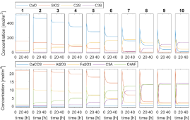
Figure 3: Dynamic evolution of solid concentrations along the kiln for a 50-hour simulation, showing the transition and steady state of nine compounds in the clinker.

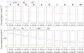
Figure 4: Dynamic evolution of gas concentrations along the kiln for a 50-hour simulation, showing the transition and steady state of 8 compounds in the gas.

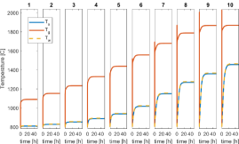
Figure 5: Dynamic evolution of temperature along the kiln for a 50-hour simulation, showing the bulk temperatures of the solid, gas, and wall phases.

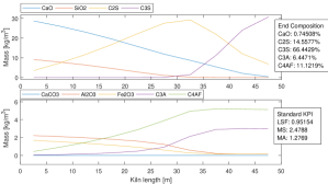
Figure 6: Steady-state mass concentrations of solid compounds along the kiln. Typical quality KPIs for the raw meal entering the kiln, as well as the resulting compound percentages in the mixture at the end of the kiln, are included.

VI Conclusion

In this paper, we presented a dynamic model of a rotary kiln for cement clinker production based on first engineering principles. The modeling focuses on the formation of clinker compounds. The model is described systematically, outlining the used thermophysical, chemical, and transportation models; enabling an easy overview of the dynamic details included, and how to extend it. The paper includes a collection of necessary property data of the different materials from the literature. The model was illustrated with a simulation, showcasing the dynamics and steady states of the kiln, resembling the expected behavior. For existing cement plants, the proposed simulation model can be used as a simplifying step in the development of advance process control systems.

References

- [1] J. Lehne and F. Preston, “Making concrete change: Innovation in low-carbon cement and concrete,” Chatham House, Tech. Rep., june 2018.
- [2] K. S. Mujumdar and V. V. Ranade, “Simulation of rotary cement kilns using a one-dimensional model,” Chemical Engineering Research and Design, vol. 84, pp. 165–177, 2006.
- [3] T. Hanein, F. P. Glasser, and M. N. Bannerman, “One-dimensional steady-state thermal model for rotary kilns used in the manufacture of cement,” Adv. Appl. Ceram., vol. 116, no. 4, pp. 207–215, 2017.
- [4] E. Mastorakos, A. Massias, C. D. Tsakiroglou, D. A. Goussis, V. N. Burganos, and A. C. Payatakes, “Cfd predictions for cement kilns including flame modelling, heat transfer and clinker chemistry,” Applied Mathematical Modelling, vol. 23, pp. 55–76, 1999.
- [5] H. A. Spang, “A dynamic model of a cement kiln,” Automatic, vol. 8, pp. 309–323, 1972.
- [6] C. Sun, J. Zhao, S. Li, and P. Jiang, “First-principle modeling and simulation of cement rotary kiln,” in 2020 Chinese Control And Decision Conference (CCDC), 2020, pp. 3267–3272.
- [7] H. Liu, H. Yin, M. Zhang, M. Xie, and X. Xi, “Numerical simulation of particle motion and heat transfer in a rotary kiln,” Powder Technology, vol. 287, pp. 239–247, 2016.
- [8] T. Ginsberg and M. Modigell, “Dynamic modelling of a rotary kiln for calcination of titanium dioxide white pigment,” Computers & Chemical Engineering, vol. 35, no. 11, pp. 2437–2446, 2011.
- [9] E. W. Weisstein. (2023, feb.) Circular segment. MathWorld–A Wolfram Web Resource. [Online]. Available: https://mathworld.wolfram.com/CircularSegment.html
- [10] D. W. Green and R. H. Perry, Eds., Perry’s Chemical Engineers’ Handbook, 8th ed. McGraw Hill, 2008.
- [11] W. C. Saeman, “Passage of solids through rotary kilns,” Chemical Engineering Progress, vol. 47, no. 10, pp. 508–514, 1951.
- [12] R. Yang, R. Zou, and A. Yu, “Microdynamic analysis of particle flow in a horizontal rotating drum,” Powder Technology, vol. 30, 2003.
- [13] K. Yamane, M. Nakagawa, S. Altobelli, T. Tanaka, and Y. Tsuji, “Steady particulate flows in a horizontal rotating cylinder,” Physics of Fluids, vol. 10, no. 6, pp. 1419–1427, June 1998.
- [14] M. N. Pedersen, “Co-firing of alternative fuels in cement kiln burners,” Ph.D. dissertation, Technical University of Denmark, 2018.
- [15] G. W. Howell and T. M. Weathers, Aerospace Fluid Component Designers’ Handbook. Volume I, Revision D. TRW Systems Group, 1970.
- [16] J. E. Hesselgreaves, R. Law, and D. A. Reay, “Chapter 1 - introduction,” in Compact Heat Exchangers, 2nd ed. Butterworth-Heinemann, 2017.
- [17] B. E. Poling, J. M. Prausnitz, and J. P. O’Connel, The Properties of Gases and Liquids. McGraw-Hill, 2001.
- [18] S. H. Tscheng and A. P. Watkinson, “Convective heat transfer in a rotary kiln,” Can. J. Chem. Eng., vol. 57, pp. 433–443, 1979.
- [19] W. Sutherland, “Lii. the viscosity of gases and molecular force,” Philosphical Magazine series 5, vol. 36, no. 223, pp. 507–531, 1893.
- [20] C. R. Wilke, “A viscosity equation for gas mixtures,” The Journal of Chemical Physics, vol. 18, no. 4, pp. 517–519, 1950.
- [21] R. Johansson, B. Leckner, K. Andersson, and F. Johnsson, “Account for variations in the \ceH2O to \ceCO2 molar ratio when modelling gaseous radiative heat transfer with the weighted-sum-of-grey-gases model,” Combustion and Flame, vol. 158, pp. 893–901, 2011.
- [22] J. P. Gorog, J. K. Brimacombe, and T. N. Adams, “Radiative heat transfer in rotary kilns,” Metall Mater Trans B, vol. 12, 1981.
- [23] Y. Guo, C. Chan, and K. Lau, “Numerical studies of pulverized coal combustion in a tubular coal combustor with slanted oxygen jet,” Fuel, vol. 82, pp. 893–907, 2003.
- [24] W. P. Jones and R. P. Lindstedt, “Global reaction schemes for hydrocarbon combustion,” Combustion and Flame, vol. 73, 1988.
- [25] S. P. Karkach and V. I. Osherov, “Ab initio analysis of the transition states on the lowest triplet \ceH2O2 potential surface,” The Journal of Chemical Physics, vol. 110, no. 24, pp. 11 918–11 927, 1999.
- [26] P. L. Walker, Char Properties and Gasification. Springer Netherlands, 1985, pp. 485–509.
- [27] P. Basu, “Chapter 7 - gasification theory,” in Biomass Gasification, Pyrolysis and Torrefaction, 3rd ed. Academic Press, 2018.
- [28] J. Rumble, Ed., CRC handbook of chemistry and physics, 103rd ed. CRC Press, 2022.
- [29] A. Ichim, C. Teodoriu, and G. Falcone, “Estimation of cement thermal properties through the three-phase model with application to geothermal wells,” Energies, vol. 11, no. 10, 2018.
- [30] A. Qomi, M. Javad, F.-J. Ulm, and R. J.-M. Pellenq, “Physical origins of thermal properties of cement paste,” Phys. Rev. Appl., vol. 3, Jun 2015.
- [31] Y. Du and Y. Ge, “Multiphase model for predicting the thermal conductivity of cement paste and its applications,” Materials, vol. 14, no. 16, 2021.
- [32] G. C. Bye, Ed., Portland Cement: Composition, Production and Properties, 2nd ed. Thomas Telford, 1999.
- [33] T. Hanein, F. P. Glasser, and M. N. Bannerman, “Thermodynamic data for cement clinkering,” Cem Concr Res, vol. 132, 2020.