0.8pt
Stability Evaluation via Distributional Perturbation Analysis
Abstract
The performance of learning models often deteriorates when deployed in out-of-sample environments. To ensure reliable deployment, we propose a stability evaluation criterion based on distributional perturbations. Conceptually, our stability evaluation criterion is defined as the minimal perturbation required on our observed dataset to induce a prescribed deterioration in risk evaluation. In this paper, we utilize the optimal transport (OT) discrepancy with moment constraints on the (sample, density) space to quantify this perturbation. Therefore, our stability evaluation criterion can address both data corruptions and sub-population shifts — the two most common types of distribution shifts in real-world scenarios. To further realize practical benefits, we present a series of tractable convex formulations and computational methods tailored to different classes of loss functions. The key technical tool to achieve this is the strong duality theorem provided in this paper. Empirically, we validate the practical utility of our stability evaluation criterion across a host of real-world applications. These empirical studies showcase the criterion’s ability not only to compare the stability of different learning models and features but also to provide valuable guidelines and strategies to further improve models.
Keywords: Model Evaluation, Distributional Perturbation, Optimal Transport
1 Introduction
The issue of poor out-of-sample performance frequently arises, particularly in high-stakes applications such as healthcare (Bandi et al.,, 2018; Wynants et al.,, 2020; Roberts et al.,, 2021), economics (Hand,, 2006; Ding et al.,, 2021), self-driving (Malinin et al.,, 2021; Hell et al.,, 2021). This phenomenon can be attributed to discrepancies between the training and test datasets, influenced by various factors. Some of these factors include measurement errors during data collection (Jacobucci and Grimm,, 2020; Elmes et al.,, 2020), deployment in dynamic, non-stationary environments (Camacho and Conover,, 2011; Conger et al.,, 2023), and the under-representativeness of marginalized groups in the training data (Corbett-Davies et al.,, 2023), among others. The divergence between training and test data presents substantial challenges to the reliability, robustness, and fairness of machine learning models in practical settings. Recent empirical studies have shown that algorithms intentionally developed for addressing distribution shifts—such as distributionally robust optimization (Blanchet et al.,, 2019; Sagawa et al.,, 2019; Kuhn et al.,, 2019; Duchi and Namkoong,, 2021; Rahimian and Mehrotra,, 2022; Blanchet et al.,, 2024), domain generalization (Zhou et al.,, 2022), and causally invariant learning (Arjovsky et al.,, 2019; Krueger et al.,, 2021) — experience a notable performance degradation when faced with real-world scenarios (Gulrajani and Lopez-Paz,, 2020; Frogner et al.,, 2021; Yang et al.,, 2023; Liu et al.,, 2023).
Instead of providing a robust training algorithm, we shift focus towards a more fundamental (in some sense even simpler) question:
Q: How do we evaluate the stability of a learning model when subjected to data perturbations?
To answer this question, our initial step is to gain a comprehensive understanding of various types of data perturbations. In this paper, we categorize data perturbations into two classes: (i) Data corruptions, which encompass changes in the distribution support (i.e., observed data samples). These changes can be attributed to measurement errors in data collection or malicious adversaries. Typical examples include factors like street noises in speech recognition (Kinoshita et al.,, 2020), rounding errors in finance (Li and Mykland,, 2015), adversarial examples in vision (Goodfellow et al.,, 2020) and, the Goodhart’s law empirically observed in government assistance allocation (Camacho and Conover,, 2011). (ii) Sub-population shifts, refer to perturbation on the probability density or mass function while keeping the same support. For example, model performances substantially degrade under demographic shifts in recommender systems (Blodgett et al.,, 2016; Sapiezynski et al.,, 2017); under temporal shifts in medical diagnosis (Pasterkamp et al.,, 2017); and under spatial shifts in wildlife conservation (Beery et al.,, 2021).
Recent investigation on the question Q predominantly centers around sub-population shifts, see (Li et al.,, 2021; Namkoong et al.,, 2022; Gupta and Rothenhaeusler,, 2023). However, in practical scenarios, it is common to encounter both types of data perturbation. Studies such as Gokhale et al., (2022) and Zou and Liu, (2023) have documented that models demonstrating robustness against sub-population shifts can still be vulnerable to data corruptions. This underscores the importance of adopting a more holistic approach when evaluating model stability, one that addresses both sub-population shifts and data corruptions.
To fully answer the question Q, we frame the model stability as a projection problem over probability space under the OT discrepancy with moment constraints. Specifically, we seek the minimum perturbation necessary on our reference measure (i.e., observed data) to guarantee that the model’s risk remains below a specified threshold. The crux of our approach is to conduct this projection within the joint (sample, density) space. Consequently, our stability metric is capable of addressing both data corruptions on the sample space and sub-population shifts on the density or probability mass space. To enhance the practical utility of our approach, we present a host of tractable convex formulations and computational methods tailored to different learning models. The key technical tool for this is the strong duality theorem provided in this paper.
To offer clearer insights, we visualize the most sensitive distribution in stylized examples. Our approach achieves a balanced and reasoned stance by avoiding overemphasis on specific samples or employing overly aggressive data corruptions. Moreover, we demonstrate the practical effectiveness of our proposed stability evaluation criterion by applying it to tasks related to income prediction, health insurance prediction, and COVID-19 mortality prediction. These real-world scenarios showcase the framework’s capacity to assess stability across various models and features, uncover potential biases and fairness issues, and ultimately enhance decision-making.
Notations. Throughout this paper, we let denote the set of real numbers, denote the subset of non-negative real numbers. We use capitalized letters for random variables, e.g., , and script letters for the sets, e.g., . For any close set , we define as the family of all Borel probability measures on . For , we use the notation to denote expectation with respect to the probability distribution . For the prediction problem, the random variable of data points is denoted by , where denotes the input covariates, denotes the target. denotes the prediction model parameterized by . The loss function is denoted as , and is abbreviated as . We use . We adopt the conventions of extended arithmetic, whereby and .
2 Model Evaluation Framework
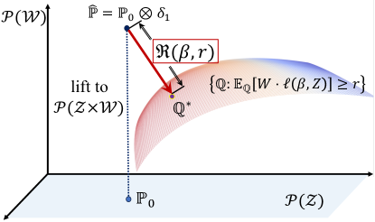
In this section, we present a stability evaluation criterion based on OT discrepancy with moment constraints, capable of considering both types of data perturbation — data corruptions and sub-population shifts — in a unified manner. The key insight lies in computing the projection distance, as shown in Figure 1, which involves minimizing the probability discrepancy between the most sensitive distribution denoted as and the lifted training distribution in the joint (sample, density) space, while maintaining the constraint that the model performance falls below a specific threshold. This threshold refer to a specific level of risk, error rate, or any other relevant performance metrics. The projection type methodology has indeed been employed in the literature for statistical inference, particularly in tasks like constructing confidence regions (Owen,, 2001; Blanchet et al.,, 2019). However, this application is distinct from our current purpose.
2.1 OT-based stability evaluation criterion
We begin by presenting the OT discrepancy with moment constraints, as proposed in Blanchet et al., (2023, Definition 2.1). This serves as a main technical tool for our further discussions.
Definition 1 (OT discrepancy with moment constraints).
If and are convex and closed sets, is a lower semicontinuous function, and , then the OT discrepancy with moment constraints induced by , and is the function defined through
where and are the marginal distributions of and under .
Remark 1.
The core idea is to lift the original sample space to a higher dimensional space —- a joint (sample, density) space. Here, we treat the additional random variable as the “density ” or “probability mass”, making it also amenable to perturbations through optimal transport methods. However, these perturbations are subject to the constraint that the expectation of the density must remain equal to one. Thus, the transportation cost function can measure the changes in both samples () and their probability densities ().
To evaluate the stability of a given learning model trained on the distribution , we formally introduce the OT-based stability evaluation criterion as
| (P) |
Here, the reference measure is selected as , with denoting the Dirac delta function,111This implies that the sample weights are almost surely equal to one with respect to the reference distribution, as we lack any prior information about them. represents the OT discrepancy with moment constraints between the projected distribution and the reference distribution , denotes the prediction risk of model on sample , and is the pre-defined risk threshold.
To sum up, we evaluate a model’s stability under distribution shifts by quantifying the minimum level of perturbations required for the model’s performance to degrade to a predetermined risk threshold. The magnitude of perturbations is determined through the use of the OT discrepancy with moment constraints and the cost function , see definition 1.
Then, a natural question arises: How do we select the cost function to effectively quantify the various types of perturbations? We aim for this cost function to be capable of quantifying changes in both the support of the distribution and the probability density or mass function. One possible candidate cost function is
| (2.1) |
Here, quantifies the cost associated with the different data samples and in the set , with the label measurement’s reliability considered infinite; denotes the cost related to differences in probability mass, where is a convex function satisfying ; serve as two hyperparameters, satisfying for some constant , to control the trade-off between the cost of perturbing the distribution’s support and the probability density or mass on the observed data points. This cost function was originally proposed in Blanchet et al., (2023, Section 5) within the framework of distributionally robust optimization.
Remark 2 (Effect of and ).
(i) When , the stability criterion only counts the sub-population shifts, as any data sample corruptions are not allowed. In this scenario, our proposed stability criterion can be reduced to the one recently introduced in Gupta and Rothenhaeusler, (2023) and Namkoong et al., (2022). (ii) When , the stability criterion only takes the data corruptions into account instead. (iii) The most intriguing scenario arises when both and have finite values. These parameters, and , hold a pivotal role in adjusting the balance between data corruptions and sub-population shifts within our stability criterion, which allows us to simultaneously consider both types of distribution shifts. By manipulating the values of and , we can achieve a versatile representation of a model’s resilience across a wide range of distributional perturbation directions. This adaptability carries significant implications when evaluating the robustness of models in diverse and ever-evolving real-world environments.
2.2 Dual reformulation and its interpretation
Problem (P) constitutes an infinite-dimensional optimization problem over probability distributions and thus appears to be intractable. However, we will now demonstrate that by first establishing a strong duality result, problem (P) can be reformulated as a finite-dimensional optimization problems and discuss the structure of the most sensitive distribution from problem (P).
Theorem 1 (Strong duality for problem (P)).
Suppose that (i) The set is compact, (ii) is upper semi-continuous for all , (iii) the cost function is continuous; and (iv) the risk level is less than the worst case value . Then we have,
| (D) |
where the surrogate function equals to
for all and .
For a detailed proof, we direct interested readers to the Appendix A.1.
Remark 3.
When the reference measure is a discrete measure, some technical conditions in Theorem 1 (e.g., compactness, (semi)-continuity) can be eliminated by utilizing the abstract semi-infinite duality theory for conic linear programs. Please refer to Shapiro, (2001, Proposition 3.4) and our proof in Appendix A.1 for more detailed information.
If we adopt the cost function in the form of (2.1) for two commonly used functions, we can simplify the surrogate function further by obtaining the closed form of . Here, we explore the following cases: (i) Selecting , which is associated with the Kullback–Leibler (KL) divergence. (ii) Choosing , which is linked to the -divergence.
Proposition 1 (Dual reformulations).
Suppose that . (i) If , then the dual problem (D) admits:
| (2.2) |
(ii) If , then the dual problem (D) admits:
| (2.3) |
where the -transform of with the step size is defined as
When the reference measure is represented as the empirical measure , the characterization of the most sensitive distribution , can be elucidated through the dual formulation provided in (2.2) and (2.3).
Remark 4 (Structure of the most sensitive distribution).
We express as follows: , where each satisfies the conditions:
Using various functions requires adjusting the weight in a distinct manner:
(i) If , then we have:
(ii) If , then we have:
where and are the optimal solution of problem (D). Therefore, it becomes evident that the most sensitive distribution encompasses both aspects of shifts: the transformation from to and the reweighting from to . Our cost function enables a versatile evaluation of model stability across a range of distributional perturbation directions. This approach yields valuable insights into the behavior of a model in different real-world scenarios and underscores the importance of incorporating both types of distributional perturbation in stability evaluation.
2.3 Computation
In this subsection, our emphasis lies in addressing problems (2.2) and (2.3) with varying types of loss functions, specifically when the reference measure takes the form of the empirical distribution.
Convex piecewise linear loss functions. If the loss function is piecewise linear (e.g., linear SVM), we can show that (2.2) admits a tractable finite convex program.
Theorem 2 (KL divergence).
Suppose that and . The negative optimal value of problem (2.2) is equivalent to the optimal value of the finite convex program:
where the set is the exponential cone defined as
Theorem 3 ( Divergnce).
Suppose that and . The negative optimal value of problem (2.2) is equivalent to the optimal value of the finite convex program
For a detailed proof, we direct interested readers to the Appendix A.3 and A.4 for more detailed information.
Equipped with Theorem 2 and 3, we can calculate our evaluation criterion by general purpose conic optimization solvers such as MOSEK and GUROBI.
0/1 loss function. In practical applications, employing a 0/1 loss function offers users a simpler method to set up the risk level , which corresponds to a pre-defined acceptable level of error rate. That is, given a trained model , we define the loss function on the sample as
where is the indicator function defined as if ; otherwise. In this scenario, the -transform of can be expressed in a closed form. Conceptually, this loss function promotes long-haul transportation, as it encourages either minimal perturbation or no movement at all, i.e.,
where .
This distance quantifies the minimal adjustment needed to fool or mislead the classifier’s prediction for the sample . A similar formulation has been employed in Si et al., (2021) to assess group fairness through optimal transport projections. Finally, the dual formulation (2.2) is reduced to an one-dimensional convex problem w.r.t .
Nonlinear loss functions. For general nonlinear loss functions, such as those encountered in deep neural networks, the dual formulation (2.2) retains its one-dimensional convex nature with respect to . However, the primary computational challenge lies in solving the inner maximization problem concerning the sample . In essence, this dual maximization problem (2.2) for nonlinear loss functions is closely associated with adversarial training (Nouiehed et al.,, 2019; Yi et al.,, 2021). All algorithms available in the literature for this purpose can be applied to our problem as well. The key distinction lies in the outer loop. In our case, we optimize over to perturb the sample weights, whereas in adversarial training, this outer loop is devoted to the training of model parameters.
For simplicity, we adopt a widely-used approach in our paper: Performing multiple gradient ascent steps to generate adversarial examples, followed by an additional gradient ascent step over . For a more thorough understanding, please see Algorithm 1. If we can solve the inner maximization problem nearly optimally, then we can ensure that the sequence generated by Algorithm 1 converges to the global optimal solution. You can find further details in Sinha et al., (2018, Theorem 2).
2.4 Feature stability analysis
As an additional benefit, if we select an alternative cost function, different from the one proposed in (2.1), our evaluation criterion can serve as an effective metric for assessing feature stability within machine learning models. If we want to evaluate the stability of the -th feature, we can modify the distance function in (2.1) as
where represents the -th feature of , while denotes all variables in except for the -th one. This implies that during evaluation, we are only permitted to perturb the -th feature while keeping all other features unchanged.
Substituting in problem (2.2), we could obtain the corresponding feature stability criterion , which provides a quantitative stability evaluation of how robust the model is with respect to changes in the -th feature. Specifically, a higher value of indicates greater stability of the corresponding feature against potential shifts.
3 Visualizations on stylized / toy examples
In this section, we use a toy example to visualize the most sensitive distribution based on Remark 4, which provides intuitive insights into the structure of .
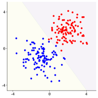
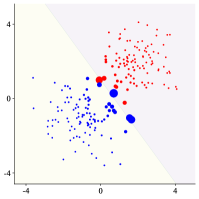
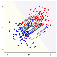
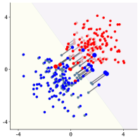
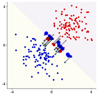
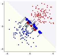
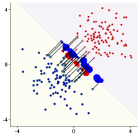
We consider a two-dimensional binary classification problem. We generate 100 samples for from distribution , and 100 samples for from distribution . The model under evaluation is logistic regression (LR). In this section, we choose . To explore the effects of varying the adjustment parameters, we fix . We use the cross-entropy loss function, set the risk threshold to be 0.5 (the original loss was 0.1), and solve the problem (2.2). In Figure 2b-2d, we visualize the most sensitive distribution in each setting, where the decision boundary of is indicated by the boundary line, colored points represent the perturbed samples, shadow points represent the original samples, and the size of each point is proportional to its sample weight in . Corresponding with the analysis in Section 2.1, we have the following observations:
-
(i)
When , our stability criterion only considers sub-population shifts. From Figure 2b, we notice a significant increase in weight assigned to a limited number of samples near the boundary. This aligns with the works of Namkoong et al., (2022); Gupta and Rothenhaeusler, (2023), which emphasize tail performance analysis.
-
(ii)
When , the stability criterion only considers data corruptions. From Figure 2c, a significant number of samples are severely perturbed to adhere to the predefined risk threshold.
-
(iii)
When , in Figure 2d, a more balanced is observed, reflecting the incorporation of both data corruptions and sub-population shifts. This showcases a scenario where samples undergo moderate and reasonable perturbations, and the sensitive distribution is not disproportionately concentrated on a limited number of samples. Such a distribution is a more holistic and reasonable approach to evaluating stability in practice, taking into account a broader range of potential shifts.
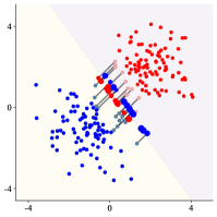
Furthermore, we showcase the most sensitive distributions with 0/1 loss. We set the error rate threshold to be 30%. The results are shown in Figure 3. From the results, we have the following observations:
-
(i)
Similar to the phenomenon above, when , the stability criterion only considers data corruptions; and when , it only considers sub-population shifts.
-
(ii)
Different from Figure 2, since we use 0/1 loss here, the perturbed samples are all near the boundary.

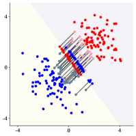

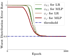
For fixed and , we vary the error rate threshold and visualize the most sensitive distribution in Figure 4. We set and , and our stability criterion will consider both data corruptions and sub-population shifts.
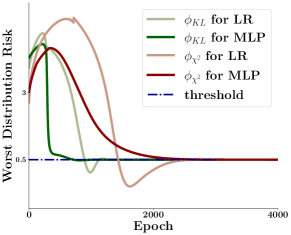
Finally, in Figure 5, we plot the curve of with respect to the epoch number . From the results, it’s evident that the infeasibility error of the sequence generated by our algorithm tends towards zero. This implies that the final expectation over the most sensitive distribution will match the predefined threshold .
4 Experiments
In this section, we explore real-world applications to show the practical effectiveness of our stability evaluation criterion, including how this criterion can be utilized to compare the stability of both models and features, and to inform strategies for further enhancements.
Datasets. We use three real-world datasets, including ACS Income dataset, ACS Public Coverage dataset, and COVID-19 dataset.
-
•
ACS Income dataset. The dataset is based on the American Community Survey (ACS) Public Use Microdata Sample (PUMS) (Ding et al.,, 2021). The task is to predict whether an individual’s income is above $50,000. We filter the dataset to only include individuals above the age of 16, usual working hours of at least 1 hour per week in the past year, and an income of at least $100. The dataset contains individuals from all American states, and we focus on California (CA) in our experiments. We follow the data pre-processing procedures in Liu et al., (2021). The dataset comprises a total of 76 features, with the majority of categorical features being one-hot encoded to facilitate analysis. In our experiments, we sample 2,000 data points from CA for model training, and another 2,000 for evaluation. When involving algorithmic interventions in Section 4.2, we further sample 5,000 points to compare the performances of different algorithms.
-
•
ACS Public Coverage dataset. The dataset is also based on ACS PUMS (Ding et al.,, 2021). The task is to predict whether an individual has public health insurance. We focus on low-income individuals who are not eligible for Medicare by filtering the dataset to only include individuals under the age of 65 and with an income of less than $30,000. Similar to the ACS Income dataset, we focus on individuals from CA in our experiments. We follow the data pre-processing procedures in Liu et al., (2021). The dataset comprises a total of 42 features, with the majority of categorical features being one-hot encoded to facilitate analysis. In our experiments, we sample 2,000 data points from CA for model training, and another 2,000 for evaluation. When involving algorithmic interventions in Section 4.2, we further sample 5,000 points to compare the performances of different algorithms.
-
•
COVID-19 dataset. The COVID-19 dataset contains COVID patients from Brazil, which is based on SIVEP-Gripe data (Baqui et al.,, 2020). It has 6882 patients from Brazil recorded between Februrary 27-May 4, 2020. There are 29 features in total, including comorbidities, symptoms, and demographic characteristics. The task is to predict the mortality of a patient, which is a binary classification problem. In our experiments, we split the dataset with a ratio of 1:1 for training and evaluation sets.
Throughout the experiments, we set for adjustment parameters and .
Algorithms under evaluation Before presenting experimental results, we will initially introduce the formulations of various algorithms used to evaluate the effectiveness of their interventions. In Section 4.1, we evaluate Adversarial Training (AT) Sinha et al., (2018) and Tilted ERM (Li et al.,, 2023). In Section 4.2, we introduce the Targeted AT. Here are their mathematical formulations:
-
(i)
AT:
(4.1) where , and is the penalty hyper-parameter.
-
(ii)
Tilted ERM:
(4.2) where is the temperature hyper-parameter.
-
(iii)
Targeted AT:
(4.3) In this case, , where denotes the target feature of , denotes all the other features and is the penalty hyper-parameter. By choosing this , the targeted AT will only perturb the target feature while keeping the others unchanged.
Training Details. In our experiments, we use LR for linear model and a two-layer MLP for neural network. We use PyTorch Library (Paszke et al.,, 2019) throughout our experiments. The number of hidden units of MLP is set to 16. As for the models under evaluation in Section 4, (i) for AT, we vary the penalty parameter and select the best according to the validation accuracy. The inner number of inner optimization iterates is set to 20; (ii) for Tilted ERM, we vary the temperature parameter and select the best according to the validation accuracy. Throughout all experiments, the ADAM optimizer with a learning rate of is used. All experiments are performed using a single NVIDIA GeForce RTX 3090.
4.1 Model stability analysis
In this section, we first provide more in-depth empirical analyses of our proposed criterion, and demonstrate how it can reflect a model’s stability with respect to data corruptions and sub-population shifts. We focus on the income prediction task for individuals from CA, using the ACS Income dataset.
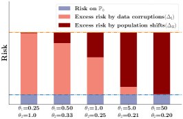
Excess risk decomposition. Recall that our stability evaluation misleads the model to a pre-defined risk threshold by perturbing the original distribution in two ways, i.e. data corruptions and sub-population shifts. Based on the optimal solutions of problem (P), we can compute the excess risk into two parts satisfying :
| (4.4) | ||||
where is the marginal distribution of w.r.t . Thus, from this decomposition, we can see that denotes the excess risk induced by data corruptions (data samples ), and denotes that induced by sub-population shifts (probability density ). In this experiment, for a MLP model trained with empirical risk minimization (ERM), we use the cross-entropy loss and set the risk threshold to be 3.0. In Figure 6a, we vary the and and plot the in each setting. The results align with our theoretical understanding that a decrease in leads our evaluation method to place greater emphasis on data corruptions. Conversely, a reduction in shifts the focus of our evaluation towards sub-population shifts. This observation confirms the adaptability of our approach in weighing different types of distribution shifts based on the values of and .
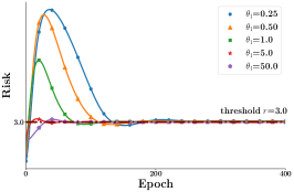
Convergence of our optimization algorithm. In Figure 6b, we plot the curve of the risk on w.r.t. the epoch number throughout the optimization process. For different values of and , we observe that the risk consistently converges to the pre-defined risk threshold of . This empirical observation is in agreement with our theoretical investigation, demonstrating the reliability and effectiveness of our optimization approach.
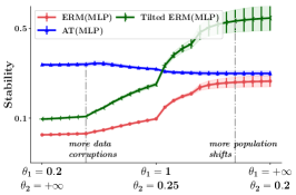
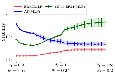
Reflection of stability. We then proceed to compare the stability of MLP models trained with three well-established methods, including ERM, AT, and Tilted ERM. AT is specifically designed to enhance the model’s resilience to data corruptions, whereas Tilted ERM, through its use of the log-sum-exp loss function, aims to prioritize samples with elevated risks, potentially enhancing stability in the presence of sub-population shifts. For our analysis, we set the risk threshold to 3.0, vary and , and plot the resulting stability measure for each method.
From Figure 6c, we have the following observations: (i) Both robust learning methods exhibit markedly higher stability compared to ERM; (ii) AT exhibits greater stability in the context of data corruptions, while Tilted ERM shows superior performance in scenarios involving sub-population shifts. These findings align with our initial hypotheses regarding the strengths of these methods; (iii) Furthermore, the results suggest that robust learning methods tailored to specific types of distribution shifts may face challenges in generalizing to other contexts. Therefore, accurately identifying the types of shifts to which a model is most sensitive is crucial in practice, as it can inform machine learning engineers on strategies to further refine and improve the model’s robustness and efficacy. This insight underscores the significance of our proposed stability evaluation framework. It offers a comprehensive and unified perspective on a model’s stability across various types of distribution shifts, enabling a more holistic understanding and strategic approach to enhancing model robustness and reliability.
Furthermore, the results of models’ stability on the ACS PubCov dataset and the COVID-19 dataset are shown in Figure 7. We can observe similar phenomenon as the ACS Income dataset:
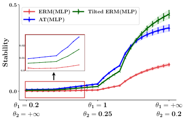
-
(i)
When is small, our stability measure pays more attention to data corruptions. Therefore, AT performs better than Tilted ERM and ERM.
-
(ii)
When is small, the main focus shifts to population shifts, where Tilted ERM is more preferred.
Besides, it is noteworthy that the standard deviation of the stability measure estimation increases as approaches infinitely (we set it to 100 in our experiments). When fixing the evaluation data, the standard deviations—indicating the randomness inherent to our computational algorithm—are relatively small. This observation points to the randomness of sampling as the primary factor. Furthermore, the introduction of brings a statistical cost in calculating the stability measure, as demonstrated in Namkoong et al., (2022).
4.2 Feature stability analysis
Building upon our previous findings, we further investigate the applicability of feature stability analysis across multiple prediction tasks, including income, insurance, and COVID-19 mortality prediction.
By examining feature stability, we gain valuable insights into the specific attributes that significantly influence model performance.
It provides a principle approach to enhance our understanding of the risky factors contributing to overall model instability, and thereby helps to discover potential discriminations and improve model robustness and fairness.
Throughout all the experiments, we use 0/1 loss function and set the error rate threshold to be .
The adjustment parameter is set to 1.0, and is 0.25.
Income prediction
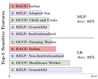
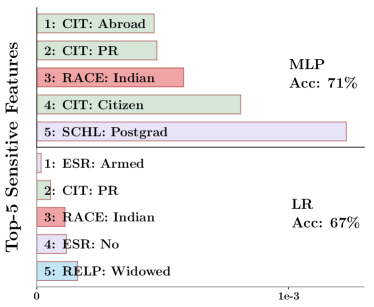
We sample 2,000 data points from ACS Income dataset for training, an additional 2,000 points for the evaluation set, and a further 5,000 points to test the effectiveness of algorithmic interventions. For both the LR model and the MLP model, trained using ERM, we use the evaluation set to compute the feature sensitivity measure for each feature as outlined in Section 2.4. The top-5 most sensitive features for each model – MLP and LR – are displayed in Figure 8a. In these visualizations, distinct colors are assigned to different types of features for clarity; for example, red is used to denote racial features, while green indicates occupation features. From the results, we observe that: (i) When the performances are similar (82% v.s. 83%), the LR model is less sensitive to input features, compared with the MLP model, which corresponds with the well-known Occam’s Razor. (ii) Interestingly, our stability criterion reveals that both the MLP and LR models exhibit a notable sensitivity to the racial feature “American Indian”. This raises concerns regarding potential racial discrimination and unfairness towards this specific demographic group. It is important to highlight that an individual’s race should not be a determinant factor in predicting their income, and the heightened sensitivity to this feature suggests a need for careful examination and potential mitigation of biases in the models before deployment.
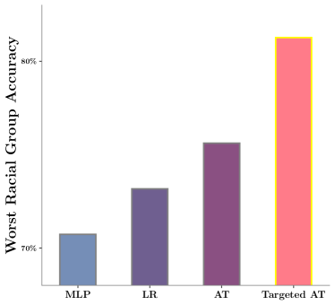
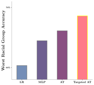
Building on our initial observations, we conduct an in-depth analysis of the accuracy across different racial groups for both the LR and MLP models. The findings, as shown in Figure 8b, align with our earlier feature stability results. Notably, the accuracy for the worst-performing racial group is significantly lower compared to other groups (for instance, a decrease from 82% to 72% in the case of the MLP model). Such findings indicate that both the LR and MLP models, when trained using ERM, exhibit unfairness towards minority racial groups. In light of these insights, our feature stability analysis serves as a valuable tool to identify and prevent the deployment of models that may perpetuate such disparities in practice.
Subsequently, we use adversarial training as an algorithmic intervention to enhance model performance.
Figure 8b illustrates the results of this intervention: AT denotes adversarial training that perturbs all racial features, whereas targeted AT specifically perturbs the identified sensitive racial feature “American Indian”.
The results indicate that targeted AT markedly outperforms all baseline models, achieving a significant improvement in accuracy for the worst-performing racial group.
This outcome effectively demonstrates the utility of our feature stability analysis in guiding targeted improvements to model performance and fairness.
Public coverage prediction
We replicated the aforementioned experiment on the ACS PubCov dataset, which involves predicting an individual’s public health insurance status. Following the previous setup, we identify and display the top-5 most sensitive features for both LR and MLP models in Figure 8c. Additionally, Figure 8d presents the accuracy for the worst-performing racial group for each method.
The findings reveal several key insights: (i) The MLP model outperforms the LR model in this context (71% vs. 67%), and it exhibits less sensitivity to input features. This observation suggests that feature sensitivity is influenced by both the nature of the task and the characteristics of the model. (ii) Consistent with previous results, the “American Indian” racial feature is identified as sensitive in both models. The accuracy of the worst-performing racial group further underscores the presence of discrimination against minority groups. (iii) Leveraging our feature stability analysis, targeted AT achieves the most notable improvement. This again underscores the effectiveness of our evaluation method in enhancing model performance and fairness.
COVID-19 mortality prediction
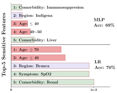
We use the COVID-19 dataset, and the task is to predict the mortality of a patient based on features including comorbidities, symptoms, and demographic characteristics. For the LR and MLP models trained with ERM, we follow the outlines in Section 2.4 and identify the top-5 most sensitive features, as shown in Figure 9a. From the results, we observe that: (i) Consistent with the trends observed in the income prediction task, the LR model demonstrates lower sensitivity to input features compared to the MLP model when their performance levels are comparable; (ii) Notably, both LR and MLP models are quite sensitive to the “Age” feature. Given the variety of risk factors for COVID-19, such as comorbidities and symptoms, it is concerning that these models might overemphasize age, which is not the sole determinant of mortality. This highlights a critical need to ensure models effectively account for diverse age groups and do not rely excessively on age as a predictive factor.
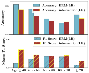
Building on these insights, we further evaluate the accuracy and macro F1 score across different age groups for the LR model. As illustrated in Figure 9, the accuracy for younger individuals (age 40) and older individuals (age 70) is notably high (the blue bars in the upper sub-figure). However, their corresponding macro F1 scores are significantly lower (as shown by the blue bars in the lower sub-figure). This suggests that the LR model may overly rely on the age feature for making predictions. For example, it tends to predict survival for younger individuals and mortality for older individuals with high probability, irrespective of other relevant clinical indicators. Such a simplistic approach raises concerns about the model’s ability to provide nuanced predictions for these age groups.
Considering the possibility of varied mortality prediction mechanisms among different age groups, we propose a targeted algorithmic intervention: training distinct LR models for each age group. From the lower sub-figure in Figure 9, we see a substantial improvement in macro F1 scores for both younger and older populations.
From these three real-world experiments, we demonstrate how the proposed feature stability analysis can help discover potential discrimination and inform targeted algorithmic interventions to improve the model’s reliability and fairness.
5 Closing Remarks
This work proposes an OT-based stability criterion that allows both data corruptions and sub-population shifts within a single framework. Applied to three real-world datasets, our method yields insightful observations into the robustness and reliability of machine learning models, and suggests potential algorithmic interventions for further enhancing model performance. The utility of our stability evaluation criterion to modern model architectures (e.g., Transformer, tree-based ensembles) and popular real-world applications (e.g., LLMs) is natural to further explore.
Impact Statements
In this paper, we propose an OT-based stability criterion that addresses the challenges posed by both data corruptions and sub-population shifts, offering a comprehensive approach to evaluating the robustness of machine learning models. The potential broader impact of this work is significant, particularly in providing a principle approach to evaluate fairness and reliability of models deployed in real-world scenarios (based on specified criteria which we take as given). By enabling more nuanced assessments of model stability, our criterion can help prevent the deployment of biased or unreliable models, thereby contributing to more equitable outcomes, especially in high-stakes applications like healthcare, finance, and social welfare. Furthermore, our work underscores the necessity of considering and mitigating potential biases and unfairness in automated decision-making systems. As machine learning continues to play an increasingly integral role in societal functions, the tools and methodologies developed in this study provide crucial steps towards ensuring that these technologies are used responsibly and ethically.
References
- Arjovsky et al., (2019) Arjovsky, M., Bottou, L., Gulrajani, I., and Lopez-Paz, D. (2019). Invariant risk minimization. arXiv preprint arXiv:1907.02893.
- Bandi et al., (2018) Bandi, P., Geessink, O., Manson, Q., Van Dijk, M., Balkenhol, M., Hermsen, M., Bejnordi, B. E., Lee, B., Paeng, K., Zhong, A., et al. (2018). From detection of individual metastases to classification of lymph node status at the patient level: the camelyon17 challenge. IEEE Transactions on Medical Imaging, 38(2):550–560.
- Baqui et al., (2020) Baqui, P., Bica, I., Marra, V., Ercole, A., and Van Der Schaar, M. (2020). Ethnic and regional variation in hospital mortality from covid-19 in brazil. The Lancet Global Health, 8(8):e1018–e1026.
- Beery et al., (2021) Beery, S., Agarwal, A., Cole, E., and Birodkar, V. (2021). The iWildCam 2021 competition dataset. arXiv preprint arXiv:2105.03494.
- Blanchet et al., (2019) Blanchet, J., Kang, Y., and Murthy, K. (2019). Robust wasserstein profile inference and applications to machine learning. Journal of Applied Probability, 56(3):830–857.
- Blanchet et al., (2023) Blanchet, J., Kuhn, D., Li, J., and Taskesen, B. (2023). Unifying distributionally robust optimization via optimal transport theory. arXiv preprint arXiv:2308.05414.
- Blanchet et al., (2024) Blanchet, J., Li, J., Lin, S., and Zhang, X. (2024). Distributionally robust optimization and robust statistics. arXiv preprint arXiv:2401.14655.
- Blanchet and Murthy, (2019) Blanchet, J. and Murthy, K. (2019). Quantifying distributional model risk via optimal transport. Mathematics of Operations Research, 44(2):565–600.
- Blodgett et al., (2016) Blodgett, S. L., Green, L., and O’Connor, B. (2016). Demographic dialectal variation in social media: A case study of african-american english. In Proceedings of the 2016 Conference on Empirical Methods in Natural Language Processing (EMNLP 2016), pages 1119–1130.
- Camacho and Conover, (2011) Camacho, A. and Conover, E. (2011). Manipulation of social program eligibility. American Economic Journal: Economic Policy, 3(2):41–65.
- Conger et al., (2023) Conger, L. E., Hoffman, F., Mazumdar, E., and Ratliff, L. J. (2023). Strategic distribution shift of interacting agents via coupled gradient flows. In Advances in Neural Information Processing Systems 36.
- Corbett-Davies et al., (2023) Corbett-Davies, S., Gaebler, J. D., Nilforoshan, H., Shroff, R., and Goel, S. (2023). The measure and mismeasure of fairness. The Journal of Machine Learning Research, 24(1):14730–14846.
- Ding et al., (2021) Ding, F., Hardt, M., Miller, J., and Schmidt, L. (2021). Retiring adult: New datasets for fair machine learning. In Advances in neural information processing systems 34, pages 6478–6490.
- Duchi and Namkoong, (2021) Duchi, J. C. and Namkoong, H. (2021). Learning models with uniform performance via distributionally robust optimization. The Annals of Statistics, 49(3):1378–1406.
- Elmes et al., (2020) Elmes, A., Alemohammad, H., Avery, R., Caylor, K., Eastman, J. R., Fishgold, L., Friedl, M. A., Jain, M., Kohli, D., Laso Bayas, J. C., et al. (2020). Accounting for training data error in machine learning applied to earth observations. Remote Sensing, 12(6):1034.
- Frogner et al., (2021) Frogner, C., Claici, S., Chien, E., and Solomon, J. (2021). Incorporating unlabeled data into distributionally robust learning. Journal of Machine Learning Research, 22(56):1–46.
- Gokhale et al., (2022) Gokhale, T., Mishra, S., Luo, M., Sachdeva, B. S., and Baral, C. (2022). Generalized but not robust? comparing the effects of data modification methods on out-of-domain generalization and adversarial robustness. In Findings of the Association for Computational Linguistics: ACL 2022, pages 2705–2718.
- Goodfellow et al., (2020) Goodfellow, I. J., Shlens, J., and Szegedy, C. (2020). Explaining and harnessing adversarial examples. In Proceedings of the 3rd International Conference on Learning Representations (ICLR 2015).
- Gulrajani and Lopez-Paz, (2020) Gulrajani, I. and Lopez-Paz, D. (2020). In search of lost domain generalization. In Proceedings of the 8th International Conference on Learning Representations (ICLR 2020).
- Gupta and Rothenhaeusler, (2023) Gupta, S. and Rothenhaeusler, D. (2023). The s-value: evaluating stability with respect to distributional shifts. In Advances in Neural Information Processing Systems 37.
- Hand, (2006) Hand, D. J. (2006). Classifier technology and the illusion of progress. Statistical Science, 21(1):1–15.
- Hell et al., (2021) Hell, F., Hinz, G., Liu, F., Goyal, S., Pei, K., Lytvynenko, T., Knoll, A., and Yiqiang, C. (2021). Monitoring perception reliability in autonomous driving: Distributional shift detection for estimating the impact of input data on prediction accuracy. In Proceedings of the 5th ACM Computer Science in Cars Symposium, pages 1–9.
- Jacobucci and Grimm, (2020) Jacobucci, R. and Grimm, K. J. (2020). Machine learning and psychological research: The unexplored effect of measurement. Perspectives on Psychological Science, 15(3):809–816.
- Kinoshita et al., (2020) Kinoshita, K., Ochiai, T., Delcroix, M., and Nakatani, T. (2020). Improving noise robust automatic speech recognition with single-channel time-domain enhancement network. In Proceedings of the 2020 IEEE International Conference on Acoustics, Speech, and Signal Processing (ICASSP 2020), pages 7009–7013. IEEE.
- Krueger et al., (2021) Krueger, D., Caballero, E., Jacobsen, J.-H., Zhang, A., Binas, J., Zhang, D., Le Priol, R., and Courville, A. (2021). Out-of-distribution generalization via risk extrapolation (rex). In Proceedings of the 38th of International Conference on Machine Learning (ICML 2021), pages 5815–5826. PMLR.
- Kuhn et al., (2019) Kuhn, D., Esfahani, P. M., Nguyen, V. A., and Shafieezadeh-Abadeh, S. (2019). Wasserstein distributionally robust optimization: Theory and applications in machine learning. In Operations research & management science in the age of analytics, pages 130–166. Informs.
- Li et al., (2021) Li, M., Namkoong, H., and Xia, S. (2021). Evaluating model performance under worst-case subpopulations. In Advances in Neural Information Processing Systems 34, pages 17325–17334.
- Li et al., (2023) Li, T., Beirami, A., Sanjabi, M., and Smith, V. (2023). On tilted losses in machine learning: Theory and applications. Journal of Machine Learning Research, 24(142):1–79.
- Li and Mykland, (2015) Li, Y. and Mykland, P. A. (2015). Rounding errors and volatility estimation. Journal of Financial Econometrics, 13(2):478–504.
- Liu et al., (2021) Liu, J., Shen, Z., He, Y., Zhang, X., Xu, R., Yu, H., and Cui, P. (2021). Towards out-of-distribution generalization: A survey. arXiv preprint arXiv:2108.13624.
- Liu et al., (2023) Liu, J., Wang, T., Cui, P., and Namkoong, H. (2023). On the need for a language describing distribution shifts: Illustrations on tabular datasets. In Thirty-seventh Conference on Neural Information Processing Systems Datasets and Benchmarks Track.
- Malinin et al., (2021) Malinin, A., Band, N., Gal, Y., Gales, M., Ganshin, A., Chesnokov, G., Noskov, A., Ploskonosov, A., Prokhorenkova, L., Provilkov, I., et al. (2021). Shifts: A dataset of real distributional shift across multiple large-scale tasks. In Thirty-fifth Conference on Neural Information Processing Systems Datasets and Benchmarks Track (Round 2).
- Namkoong et al., (2022) Namkoong, H., Ma, Y., and Glynn, P. W. (2022). Minimax optimal estimation of stability under distribution shift. arXiv preprint arXiv:2212.06338.
- Nouiehed et al., (2019) Nouiehed, M., Sanjabi, M., Huang, T., Lee, J. D., and Razaviyayn, M. (2019). Solving a class of non-convex min-max games using iterative first order methods. In Advances in Neural Information Processing Systems 32.
- Owen, (2001) Owen, A. B. (2001). Empirical Likelihood. CRC press.
- Pasterkamp et al., (2017) Pasterkamp, G., Den Ruijter, H. M., and Libby, P. (2017). Temporal shifts in clinical presentation and underlying mechanisms of atherosclerotic disease. Nature Reviews Cardiology, 14(1):21–29.
- Paszke et al., (2019) Paszke, A., Gross, S., Massa, F., Lerer, A., Bradbury, J., Chanan, G., Killeen, T., Lin, Z., Gimelshein, N., Antiga, L., et al. (2019). Pytorch: An imperative style, high-performance deep learning library. In Advances in neural information processing systems 32.
- Rahimian and Mehrotra, (2022) Rahimian, H. and Mehrotra, S. (2022). Frameworks and Results in Distributionally Robust Optimization. Open Journal of Mathematical Optimization.
- Roberts et al., (2021) Roberts, M., Driggs, D., Thorpe, M., Gilbey, J., Yeung, M., Ursprung, S., Aviles-Rivero, A. I., Etmann, C., McCague, C., Beer, L., et al. (2021). Common pitfalls and recommendations for using machine learning to detect and prognosticate for covid-19 using chest radiographs and ct scans. Nature Machine Intelligence, 3(3):199–217.
- Sagawa et al., (2019) Sagawa, S., Koh, P. W., Hashimoto, T. B., and Liang, P. (2019). Distributionally robust neural networks. In Proceedings of the 7th International Conference on Learning Representations (ICLR 2019).
- Sapiezynski et al., (2017) Sapiezynski, P., Kassarnig, V., Wilson, C., Lehmann, S., and Mislove, A. (2017). Academic performance prediction in a gender-imbalanced environment. In FATREC Workshop on Responsible Recommendation Proceedings.
- Shapiro, (2001) Shapiro, A. (2001). On duality theory of conic linear problems. In Semi-infinite programming, pages 135–165. Springer.
- Si et al., (2021) Si, N., Murthy, K., Blanchet, J., and Nguyen, V. A. (2021). Testing group fairness via optimal transport projections. In Proceedings of the 38th International Conference on Machine Learning (ICML 2021), pages 9649–9659.
- Sinha et al., (2018) Sinha, A., Namkoong, H., and Duchi, J. (2018). Certifying some distributional robustness with principled adversarial training. In Proceedings of the 6th International Conference on Learning Representations (ICLR 2018).
- Van der Vaart, (2000) Van der Vaart, A. W. (2000). Asymptotic Statistics, volume 3. Cambridge university press.
- Wynants et al., (2020) Wynants, L., Van Calster, B., Collins, G. S., Riley, R. D., Heinze, G., Schuit, E., Albu, E., Arshi, B., Bellou, V., Bonten, M. M., et al. (2020). Prediction models for diagnosis and prognosis of covid-19: systematic review and critical appraisal. bmj, 369.
- Yang et al., (2023) Yang, Y., Zhang, H., Katabi, D., and Ghassemi, M. (2023). Change is hard: A closer look at subpopulation shift. In Proceedings of the 40th International Conference on Machine Learning (ICML 2023), pages 39584–39622.
- Yi et al., (2021) Yi, M., Hou, L., Sun, J., Shang, L., Jiang, X., Liu, Q., and Ma, Z. (2021). Improved ood generalization via adversarial training and pretraing. In Proceedings of the 38th International Conference on Machine Learning (ICML 2021), pages 11987–11997.
- Zhou et al., (2022) Zhou, K., Liu, Z., Qiao, Y., Xiang, T., and Loy, C. C. (2022). Domain generalization: A survey. IEEE Transactions on Pattern Analysis and Machine Intelligence.
- Zou and Liu, (2023) Zou, X. and Liu, W. (2023). On the adversarial robustness of out-of-distribution generalization models. In Advances in Neural Information Processing Systems 37.
Appendix A Proofs
A.1 Proof of Theorem 1
Proof.
To start with, we first reformulation the primal problem (P) into an infinite-dimensional linear program:
| (Primal) |
We aim to apply Sion’s minimax theorem to the Lagrangian function
where , , and belongs to the primal feasible set
Since is compact, it follows that is tight. Furthermore, as a subset of a tight set is also tight, we conclude that is tight as well. Consequently, according to Prokhorov’s theorem (Van der Vaart,, 2000, Theorem 2.4), has a compact closure. By taking the limit in the marginal equation, we observe that is weakly closed, establishing that is indeed compact. Moreover, it can be readily demonstrated that is convex.
The Lagrangian function is linear in both and . To employ Sion’s minimax theorem, we will now prove that (i) is lower semicontinuous in under the weak topology and (ii) continuous in under the uniform topology in .
(i) Suppose that converges weakly to . Then, Portmanteau theorem states that for any lower semicontinuous function that is bounded below, we have
Since is upper semicontinuous for all and , we can conclude that is upper semicontinuous w.r.t . Moreover, armed with the lower semicontinuity of the function , we know the following candidate function
is lower semicontinuous with respect to for any . As is compact, the above candidate function is also bounded below. Thus, we have
It follows that is lower semicontinuous in under the weak topology.
(ii) Suppose now that in the Euclidean topology and in the Euclidean topology. There exists and with and for all . Thus, by the dominated convergence theorem, we have
We then conclude that is continuous in under the Ecludiean topology in .
We are now prepared to utilize Sion’s minimax theorem, and thus, we have:
| (A.1) |
Our subsequent task involves demonstrating the equivalence between the left-hand side of (A.1) and the primal problem (Primal). To achieve this, we will re-express the function as follows:
Then, we can see is bounded above. To start with, we construct a single support distribution as follows: where . Then, we have
where the second inequality follows from and the last equality holds as we know and is continuous and hence bounded on a compact domain . For any feasible point , let us consider the inner supremum of the left-hand-side of (A.1), ensuring it doesn’t go to infinity. In this case, we find that
It remains to be shown that the sup-inf part is equivalent to the dual problem (D). To do this, we rewrite the dual problem as
The last step is to take the supremum of over . That is,
due to the measurability of functions of the form , following the similar argument in (Blanchet and Murthy,, 2019). ∎
When the reference measure is discrete, i.e., , we can get the strong duality result under some mild conditions.
Theorem 4 (Strong duality for problem (P)).
Suppose that holds. Then we have,
| (D) |
A.2 Proof of Proposition 1
Proof.
Now, we are trying to calculate the surrogate function with our proposed cost function in (2.1) . Then, we have
where the first equality follows as almost surely and , and the second equality holds due to the definition of conjugate functions.
(i) When and , we know its conjugate function . Consequently, we obtain the following:
where the second equality follows from the fact the function is monotonically increasing. Hence, we can reformulate the dual problem (D) as
Next, we will solve the supremum problem via and the first-order condition reads
and . Put all of them together, we get
(ii) When and , the conjugate function can be computed as . Additionally, it is straightforward to demonstrate that is a monotonically increasing function. Hence, we have:
where the third equality holds as the monotonicity of . Then, we can reduce the dual problme (D) as
∎
Remark 5.
We want to highlight the distinction between the KL and -divergence cases. In the latter case, we are unable to derive a closed-form expression for the optimal . Instead, we must reduce it to a solution of a piecewise linear equation as follows:
| (A.3) |
A.3 Proof of Theorem 2
Proof.
By introducing epigraphical auxiliary variable , we know problem (2.2) is equivalent to
| (A.7) | ||||
| (A.12) | ||||
| (A.18) |
Here, the second equality can be derived from the fact that the second inequality in problem (A.7) can be reformulated as
To handle this constraint, we introduce an auxiliary variable , allowing us to further decompose it into exponential cone constraints and one additional linear constraint. Specifically, we have
The third constraint can be further reduced to (A.4) by considering the fact that the set corresponds to the exponential cone, which is defined as
The fourth equality is due to when we introduce auxiliary variables .
Next, we show that admits the following equivalent forms
| (A.19) | ||||
where the second equivalence arises from the non-negativity of , while the third one can be derived from the nature of the cost function, which is defined as . The second term in the cost function prevents us from perturbing the label due to the imposed budget limit.
Put everthing together, we have
∎
A.4 Proof of Theorem 3
Appendix B Pseudo-code for Algorithms
In this section, we provide the pseudo-code of our algorithms. For , please refer to Algorithm 1, and for , please see Algorithm 2.
| (B.1) |