DeepMpMRI: Tensor-decomposition Regularized Learning for Fast and High-Fidelity Multi-Parametric Microstructural MR Imaging

Abstract

Deep learning has emerged as a promising approach for learning the nonlinear mapping between diffusion-weighted MR images and tissue parameters, which enables automatic and deep understanding of the brain microstructures. However, the efficiency and accuracy in the multi-parametric estimations are still limited since previous studies tend to estimate multi-parametric maps with dense sampling and isolated signal modeling. This paper proposes DeepMpMRI, a unified framework for fast and high-fidelity multi-parametric estimation from various diffusion models using sparsely sampled q-space data. DeepMpMRI is equipped with a newly designed tensor-decomposition-based regularizer to effectively capture fine details by exploiting the correlation across parameters. In addition, we introduce a Nesterov-based adaptive learning algorithm that optimizes the regularization parameter dynamically to enhance the performance. DeepMpMRI is an extendable framework capable of incorporating flexible network architecture. Experimental results demonstrate the superiority of our approach over 5 state-of-the-art methods in simultaneously estimating multi-parametric maps for various diffusion models with fine-grained details both quantitatively and qualitatively, achieving 4.5 - 22.5$\times$ acceleration compared to the dense sampling of a total of 270 diffusion gradients.

diffusion MRI, microstructure estimation, tensor-SVD, adaptive learning

1 Introduction

Diffusion MRI (dMRI) plays a vital role in characterizing in vivo brain microstructures non-invasively. Diffusion-weighted images (DWIs) are sensitive to the random displacement of water molecules within a voxel, probing tissue on scales significantly lower than image resolution [1]. The diffusion MR signal in a voxel is considered a composite of signals from various compartments. By carefully designing signal models that relate tissue microstructure to diffusion signals, the organization of the neuronal tissue can be inferred from the observed measurements by model fitting [2]. The capability to detect subtle changes in brain tissue is particularly crucial in establishing biomarkers for the early-stage diagnosis of neurodegenerative diseases [3, 4].

Diffusion tensor imaging (DTI) stands out as the most commonly used model in diffusion MRI [5, 6]. DTI-derived metrics, including fractional anisotropy (FA), mean diffusivity (MD), and axial diffusivity (AD) [7], are commonly used as surrogate measures of microstructural tissue changes. These metrics provide valuable insights into microstructural changes associated with normal aging [8], neurodegeneration [9], and neurological diseases [10, 11]. Nonetheless, the oversimplification of the diffusion tensor model renders DTI measures biologically nonspecific [12], where different biological processes may lead to similar changes in DTI measures [12]. Consequently, tracing the source of observed signal abnormalities presents a challenge—whether they stem from intrinsic alterations in the tissue microstructure or deviations in the neural circuitry [13, 14].

To enhance the specificity of dMRI, more advanced signal models have been proposed, including Intravoxel Incoherent Motion (IVIM) model [15, 16], AxCaliber model [17], the Spherical Mean Technique (SMT) model [18], and the Neurite Orientation Dispersion and Density Imaging (NODDI) model [19]. For example, the NODDI model distinguishes three microstructural environments: intra-neurite, extra-neurite, and cerebrospinal fluid (CSF) compartments, thus enhancing the sensitivity of diffusion MRI to changes in brain tissue and providing specific markers that reflect tissue microstructure. The rotationally invariant scalar measures [20] derived from the NODDI model have been applied in numerous neuroscientific studies.

Due to the complicated model design, the advanced signal models beyond DTI usually require prolonged imaging protocols with a large number of diffusion samples. The reliable estimation of tissue microstructure described by these models may require close to or more than 100 diffusion gradients with multiple b-values [19, 13, 18]. Thus, in clinical settings where a reduced number of diffusion samples are acquired, accomplishing accurate estimation of tissue microstructure described by these advanced signal models can be challenging [12, 21, 22]. Furthermore, the raw diffusion data often suffer from Rician noise and eddy current, especially in high-b-value imaging [23], resulting in a reduction in the signal-to-noise ratio (SNR) and further degradation of the accuracy of subsequent quantitative imaging and analysis.

Recently, deep learning has exhibited remarkable success across various domains and has shown potential in microstructure estimation with fewer measurements. The q-space deep learning (q_DL) [24], was the first to directly map dMRI signals to microstructural parameters using a limited number of q-space samples through a multilayer perceptron (MLP). Note that Golkov et al.[24] suggested using a separate MLP for each microstructure parameter. Then convolutional neural networks (CNNs) were also utilized to predict high-quality scalar diffusion metrics using a small amount of diffusion data [25, 26, 27]. Beyond the data-driven mapping approaches, model-based neural networks incorporating domain knowledge have been introduced to improve network performance and interpretability. Specifically, the model-based neural network is designed by unfolding the conventional optimization process of a mathematical model to construct deep networks. For example, inspired by accelerated microstructure imaging via convex optimization (AMICO) [28], Ye et al. [29, 30] proposed patch-wise dictionary-based DL approaches to estimate parametric diffusion maps of NODDI and the multi-compartment SMT separately. Chen et al. [31, 32] used a subset q-space to estimate the NODDI parameters by explicitly considering the q-space geometric structure with a graph neural network.

Leveraging multiple microstructural features from different diffusion models contributes to a more comprehensive understanding of brain microstructure. As presented in Figure 1, multiple microstructural parameters from different diffusion models rely on the same biological tissue, sharing the same anatomical and diffusion information, thus demonstrating high correlation. However, despite the promising achievements, the efficiency and accuracy of multi-parametric estimations remain limited as previous deep learning-based studies have primarily focused on estimating multi-parametric maps individually using isolated signal modeling. Although some research has employed multi-parametric learning [25, 33, 34, 35], they tend to directly output multiple parameters without considering the correlation among parameters.

To address these challenges, we propose a deep learning-based framework for diffusion MRI named DeepMpMRI, which simultaneously estimates multiple microstructural parameters derived from various diffusion models. DeepMpMRI incorporates a newly designed tensor-decomposition-based regularization (TDR) to exploit the correlation among multiple parameters derived from different models. TDR preserves the inherent high-dimensional structure of multi-parameter tensors and utilizes tensor-SVD [36, 37, 38] to uncover the relationship between them, enhancing the performance of microstructure estimation. Additionally, the weighting hyperparameter should be properly selected since it greatly impacts network performance. However, the process of hyperparameter selection typically involves time-consuming tuning. Thus, we introduce a Nesterov-based [39] adaptive learning algorithm that optimizes the regularization parameter dynamically to further enhance performance and streamline the optimization process.

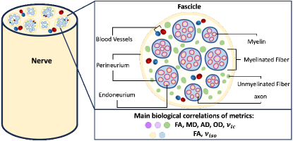
Figure 1: Schematic illustration of multi-parametric correlation in the nerve cross-sectional anatomy. The main biological compartments underlying these multiple parameters are myelin, intra-axonal space (in both myelinated and unmyelinated fibers), and extra-axonal space. Parameters can also be influenced by surrounding tissue compartments.

Overall, the main contributions of our work are as follows:

• We propose a unified framework named DeepMpMRI to facilitate high-fidelity multi-parametric estimation for various diffusion models using sparsely sampled q-space data. DeepMpMRI is a highly extendable framework that can accommodate diverse diffusion models and utilize flexible network architecture as the backbone.

• We design a novel tensor-decomposition-based regularization (TDR) to exploit the underlying high-order correlations shared among multiple parameters. The TDR specifically targets the alignment between predicted multiple parameters and ground truth in tensor singular subspace, effectively capturing fine-grained details while suppressing noise.

• We propose a Nesterov-based adaptive learning algorithm (NALA) that optimizes the regularization parameter dynamically, enabling more efficient hyperparameter tuning and better performance. Experiments indicate that our method outperforms 5 state-of-the-art methods both quantitatively and qualitatively.

The rest of the paper is organized as follows. Section 2 states the problem definition and describes the proposed framework in detail. Section 3 presents experiments conducted on the HCP dataset. In Section 4 and 5, the experiments’ results and discussion are given. Finally, Section 6 concludes the paper.

2 MATERIAL AND METHOD

This section provides a concise overview of the basic notations used in this paper, followed by a statement of the problem and a detailed presentation of the proposed DeepMpMRI. The proposed method is depicted in Fig. 2 and encompasses key elements, specifically the tensor-decomposition-based regularization (TDR) and the Nesterov-based adaptive learning algorithm (NALA).

As illustrated in Fig. 2, the overall architecture consists of two branches, with the upper branch representing the ground truth acquisition from dense sampling, while the lower branch symbolizes the network prediction from the sparse sampling. The network input is sparse measurements uniformly sampled from the dense measurements using DMRITool [40, 41], and tensor Singular Value Decomposition (t-SVD) [36, 37, 38] is applied to both network prediction and ground truth to further align them within the tensor singular subspace.

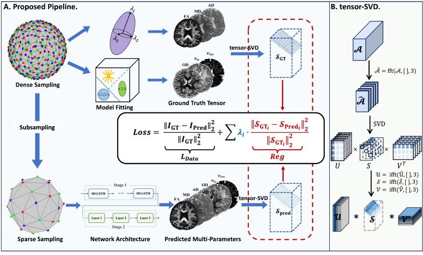
Figure 2: An illustration of the proposed DeepMpMRI framework. Left: The whole architecture consists of two branches, with the upper branch being the Ground Truth acquisition from the dense sampling and the lower branch being the network prediction from the sparse sampling. The input of the framework is sparse measurements uniformly sampled at each shell from the dense measurements, and tensor Singular Value Decomposition (t-SVD) is applied to both network prediction and ground truth to further align them within the tensor singular subspace. Right: The flowchart of tensor-SVD implementation. For detailed information, please refer to [36, 37, 38, 42, 43].

2.1 Notation and Material

This paper uses the commonly used notation where tensor with a capital calligraphic letter $\mathbf{\mathcal{A}}$, is a multidimensional array. If $\mathbf{\mathcal{A}}$ is a tensor of order-$p$, then can be written as $\mathbf{\mathcal{A}}=\left(\mathbb{\mathit{a}}_{\mathbb{\mathit{i}}_{1}\mathbb{\mathit{i}}_{2}\ldots\mathbb{\mathit{i}}_{\mathbb{\mathit{p}}}}\right)\in\mathbb{R}^{n_{1}\times n_{2}\times\cdots\times n_{p}}$. A matrix (order-$2$ tensor) is denoted with a bold capital letter, $\mathbb{\mathit{\textbf{A}}}\in\mathbb{R}^{n_{1}\times n_{2}}$, a vector (order-$1$ tensor) is denoted with a bold lowercase letter, $\mathbb{\mathit{\textbf{a}}}\in\mathbb{R}^{n_{1}\times 1}$, and scalar (order-$0$ tensor) is denoted by a lowercase letter, $a\in R$.

There exist several well-known methods to decompose a high order tensor $\mathbf{\mathcal{A}}$: CANDECOMP/PARAFAC (CP) [44, 45], Tucker [46], higher-order SVD (HOSVD) [47], Tensor-Train [48] and tensor SVD [36, 37, 38]. Among these definitions, only tensor-SVD satisfies an Eckart-Young-like Theorem, which parallels that of the matrix SVD [42, 43]. The mathematical definition and computation of the tensor-SVD are beyond the scope of this paper. For detailed information, please refer to [36, 37, 38, 42, 43].

2.2 Problem Definition of Microstructure parameter estimation

By applying a set of diffusion gradients, we can acquire a vector of diffusion signals at each voxel. Each diffusion signal can be considered as a set of $W\times H\times S$ size volumes captured in the q-space. Thus the dMRI data are 4D signals of size $\mathbb{R}^{W\times H\times S\times D}$, where $W$, $H$, $S$, $D$ refer to the width, height, slice, and gradient directions, respectively.

We aim to estimate the multiple parameters derived from various diffusion models using sparsely sampled q-space data. Given the diffusion MRI data $\mathcal{X}\in\mathbb{R}^{W\times H\times S\times D_{Full}}$, containing the full measurements in the q-space, we can obtain the corresponding ground-truth scalar maps $\mathcal{Y}_{GT}$ by model fitting. The network $\mathcal{F}_{\theta}$ parameterized by $\theta$ is designed to learn a mapping from the given sparse sampling data $\widetilde{\mathcal{X}}{\in\mathbb{R}}^{W\times H\times S\times D_{Sparse}}$ to predicted multi-parameters $\mathcal{Y}$ s.t. $\mathcal{Y}=\mathcal{F}_{\theta}(\widetilde{\mathcal{X}})\rightarrow\mathcal{Y}_{GT}$.

It has been recently shown that parameter estimation is challenging under normal experimental conditions [49, 50, 51]. Fitting these models with noisy measurements is generally a non-convex optimization problem, potentially having several local minima of the objective function. Jelescu et. al. [49] evidenced the estimation is an ill-posed inverse problem for clinically feasible dMRI acquisitions. To tackle this problem, prior knowledge was introduced as a regularization term to constrain the solution:

$$\min_{\theta}L_{Data}(\mathcal{F}_{\theta}(\widetilde{\mathcal{X}}),\mathcal{Y}_{GT})+\lambda\cdot R_{\theta}(\widetilde{\mathcal{X}})$$ (1)

where $L_{Data}(\cdot)$ denotes the data fidelity between the network output $\mathcal{F}_{\theta}(\widetilde{\mathcal{X}})$ and ground truth $\mathcal{Y}_{GT}$, $R_{\theta}(\cdot)$ is the regularization applied to the input $\widetilde{\mathcal{X}}$, , such as sparsity [52, 53, 54, 55], low-rank [52, 56, 57, 58], total variation (TV) [59, 56, 60] regularization, etc. The hyper-parameter $\lambda$ is a scalar determining how strongly the prior knowledge will be weighted during estimation.

2.3 DeepMpMRI

2.3.1 Tensor-decomposition-based regularization

Most existing regularization strategies only consider the properties of the diffusion signal and apply the regularization term to the raw dMRI data rather than the desired microstructural parameters. To facilitate accurate and fine-grained reconstruction of microstructure, we explicitly consider the quality of derived parameters in the overall optimization problem:

$$\min_{\theta}L_{Data}(\mathcal{F}_{\theta}(\widetilde{\mathcal{X}}),\mathcal{Y}_{GT})+\lambda\cdot R(\mathcal{F}_{\theta}(\widetilde{\mathcal{X}}),\mathcal{Y}_{GT})$$ (2)

here $\textit{R}(\cdot)$ is the regularization over the given predicted metrics $\mathcal{F}_{\theta}(\widetilde{\mathcal{X}})$.

To simultaneously estimate multiple parameters from various diffusion model, a multi-head deep network is employed to explore inter-model complementary information and fuse the two diffusion representations and their derived high-level features within the network. The objective function is partly defined based on the network output to enforce the consistency between the predicted and the ground truth scalar maps $\mathcal{Y}_{GT}$ obtained from the full sampling. The loss term for data is defined as:

$$L_{Data}=\frac{\left\|\mathcal{Y}_{GT}-\mathcal{Y}\right\|_{2}^{2}}{\left\|\mathcal{Y}_{GT}\right\|_{2}^{2}}$$ (3)

As an extension of the Singular Value Decomposition (SVD), the tensor-SVD expands the capability to capture data correlations in multiple dimensions beyond the typical 2D spatial domain. We maintain the dimensional coherence of the multiple parameters and utilize tensor-SVD to capture shared anatomical and diffusion information embedded in the high-dimensional parameters to enhance estimation performance. After obtaining the network output we further apply t-SVD on both the predicted multi-parameter tensor and the ground truth tensor, ensuring data consistency in the tensor singular subspace. The regularization is defined as:

$$R=\frac{\left\|\text{tSVD}(\mathcal{Y}_{GT})-\text{tSVD}(\mathcal{Y})\right\|_{2}^{2}}{\left\|\text{tSVD}(\mathcal{Y}_{GT})\right\|_{2}^{2}}=\frac{\left\|\mathcal{S}_{GT}-\mathcal{S}\right\|_{2}^{2}}{\left\|\mathcal{S}_{GT}\right\|_{2}^{2}}$$ (4)

where $\mathcal{S}$ and $\mathcal{S}_{GT}$ refer to the singular value tensors of ground truth $\mathcal{Y}_{GT}$ and prediction $\mathcal{Y}$ respectively.

The Eckart–Young theorem [61, 62] suggests that the majority of the informational content in a matrix is captured by the dominant singular subspaces (i.e., the span of the singular vectors corresponding to the largest singular values) [43]. This principle extends to tensors as well. The principal tensor singular subspace encapsulates the primary information of the microstructure parameters, whereas the components associated with smaller tensor singular values may contain noise. As a result, our focus is primarily on aligning the primary tensor singular values to ensure consistency in the extraction of significant information, effectively preserving fine details while reducing noise.

The total loss is the weighted combination of the above two loss terms:

$$L =L_{Data}+\lambda\cdot R(\cdot)$$ (5)

$$=\frac{\left\|\mathcal{Y}_{GT}-\mathcal{Y}\right\|_{2}^{2}}{\left\|\mathcal{Y}_{GT}\right\|_{2}^{2}}+\lambda\cdot\frac{\left\|\mathcal{S}_{GT}-\mathcal{S}\right\|_{2}^{2}}{\left\|\mathcal{S}_{GT}\right\|_{2}^{2}}$$

where the hyper-parameter $\lambda$ balances the contribution between data fitting and prior knowledge. A $\lambda$ value of 0 indicates that the prior knowledge does not influence the estimation. In this scenario, the network solely learns the mapping between diffusion-weighted images and multiple parameters from training data without considering their correlations. Conversely, as $\lambda$ increases, the optimization places greater emphasis on extracting dominant information, potentially overlooking the subtleties embedded in the raw data. Hence, the weighting hyperparameter should be properly selected.

2.3.2 Nesterov-based Adaptive Learning Algorithm

The process of hyperparameter selection is in practice often based on trial-and-error and grid or random search [63], which can be a time-consuming process. In contrast, Baydin et al.[64] drew inspiration from the work of Almeida et al. [65] and proposed updating hyperparameters at each step of the optimization process. Additionally, Martínez-Rubio et al. [66] provide convergence analysis for this method, further validating its effectiveness.

Thus, building upon the foundation laid by previous studies, we propose a Nesterov-based hyperparameter Adaptive Learning Algorithm (NALA). Our method optimizes the network parameter $\theta$ and hyperparameter $\lambda$ alternately on the training and validation sets, respectively. Let $\lambda_{t}$ and $\theta_{t}$ be the values of $\lambda$ and $\theta$ at the step $t$. More specifically, the iterations go as follows:

$$\left\{\begin{aligned} L(\theta,\lambda)&=L_{Data}(\theta)+\lambda\cdot R(\theta)\\ \text{On Training Set: }\theta_{t+1}&=\arg\min_{\theta}{L(\theta,\lambda_{t})}\\ \text{On Validation Set: }\lambda_{t+1}&=\arg\ \min_{\lambda}{L(\theta_{t+1},\lambda)}\end{aligned}\right.$$ (6)

In analogy to updating network parameter $\theta$, $\lambda_{t}$ should be updated in the direction of the gradient of the loss $L(\theta_{t},\lambda_{t})$ concerning $\lambda_{t}$, scaled by another hyper-hyperparameter $\beta$. One way to compute $\frac{\partial L(\theta_{t+1},\lambda_{t})}{\partial\lambda_{t}}$ is the direct manual computation of the partial derivative:

$$\frac{\partial L\left(\theta_{t+1},\lambda_{t}\right)}{\partial\lambda_{t}}=\frac{\partial\left[L_{Data}\left(\theta_{t+1}\right)+\lambda_{t}\cdot R(\theta_{t+1})\right]}{\partial\lambda_{t}}=R(\theta_{t+1})$$ (7)

where Eq. 7 can be obtained by observing that $L_{Data}(\theta_{t})$ and $R(\theta_{t})$ do not depend on $\lambda_{t}$. This expression lends itself to a simple and efficient implementation: simply remember the past regularization value. By leveraging insights from the Nesterov accelerated gradient [39], which has a provably bound for convex, non-stochastic objectives, we introduce an improved momentum term $m$ here:

$$m_{t+1}=\beta\cdot m_{t}+R(\theta_{t+1})+\beta\cdot\left[R(\theta_{t+1})-R(\theta_{t})\right]$$ (8)

where $R(\theta_{t+1})-R(\theta_{t})$ is the differential of the gradient, which approximates the second-order derivative of the objective function. Thus, the improved momentum term now averages the past search directions $m_{t}$, the current stochastic gradient $R_{t}$ and the approximate second-order derivative to determine the search direction $m_{t+1}$.

Therefore, the update rule is:

$$\lambda_{t+1} =\lambda_{t}-\alpha\cdot m_{t+1}$$ (9)

$$=\lambda_{t}-\alpha\beta\cdot m_{t}-\alpha\cdot R(\theta_{t+1})-\alpha\beta\cdot\left[R(\theta_{t+1})-R(\theta_{t})\right]$$

During the initial training phase, a significant disparity exists between the predicted and ground truth tensors. As a result, $\lambda$, determined by Eq. 9, assumes a relatively large value, which facilitates the acceleration of network training. As the training process nears completion, the disparity between the predicted and ground truth becomes smaller, leading to a gradual decrease in lambda towards convergence. Our proposed algorithm operates with minimal memory usage and minimal computational overhead, requiring only a single extra past regularization copy and only one step to update.

Algorithm 1 Nesterov-based Adaptive Learning Algorithm

0:  $\lambda_{0}$: The initial parameters;$\alpha$: The hyper-hyperparameters;$\beta$: The momentum coefficient, usually set to 0.9;$m_{0}$: The initial momentum, set to 0;

0:  $\lambda_{t+1}$

  while not converged do

     $t+1\leftarrow t$;$\theta_{t+1}\leftarrow\arg\min_{\theta}{L(\theta,\lambda_{t})}$;$m_{t+1}\leftarrow\beta\cdot m_{t}+R(\theta_{t+1})+\beta\cdot\left[R(\theta_{t+1})-R(\theta_{t})\right]$;$\lambda_{t+1}\leftarrow\lambda_{t}-\alpha\cdot m_{t+1}$;

  end while

  return  $\lambda_{t+1}$

2.4 Backbone Network

Note that DeepMpMRI is a flexible framework and can utilize any network architecture suitable for the task. Here, the Microstructure Estimation with Sparse Coding using Separable Dictionary (MESC-SD) [30], an unfolding network is employed as our backbone. MESC-SD adaptively incorporates historical information with spatial-angular sparse coding, and it is achieved by modified long short-term memory (LSTM) units [67]. MESC-SD consists of two cascaded stages, the first stage computes the spatial-angular sparse representation of the diffusion signal while the second stage maps the sparse representation to tissue microstructure estimates.

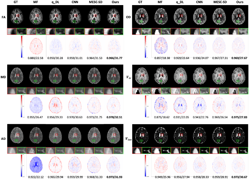
Figure 3: The ground truth, estimated parameters (FA, MD, AD, OD, $V_{ic}$, $V_{iso}$) and corresponding error maps based on Model Fitting (MF), q_DL, CNN, MESC-SD, and Ours in a test subject with 6 diffusion directions per shell at b-values of 1000, 2000, and 3000 $s/{mm}^{2}$.

Table 1: The quantitative results were obtained with 6 diffusion directions per shell at b-values of 1000, 2000, and 3000 $s/{mm}^{2}$ compared to Model Fitting (MF), q_DL, CNN and MESC-SD in terms of SSIM and PSNR. The best results are in bold.

Methods	SSIM
(18 DWIs)	FA	MD	AD	OD	$V_{ic}$​​	$V_{iso}$​​	All
MF	0.8635	0.9408	0.8978	0.8506	0.8738	0.9491	0.8961
q_DL	0.9377	0.9448	0.9584	0.9146	0.9152	0.9315	0.9337
CNN	0.9498	0.9635	0.9492	0.9267	0.9361	0.9417	0.9445
MESC-SD	0.9555	0.9665	0.9601	0.9609	0.9654	0.9506	0.9586
Ours	0.9575	0.9724	0.9658	0.9635	0.9722	0.9635	0.9658
Methods	PSNR
(18 DWIs)	FA	MD	AD	OD	$V_{ic}$​​	$V_{iso}$​​	All
MF	21.7878	25.8260	21.8471	18.6255	18.7381	25.9356	21.2090
q_DL	28.9136	28.9227	29.6672	22.9375	21.3020	26.5485	25.1443
CNN	29.7687	29.7283	30.0094	24.7241	23.8578	27.6486	27.1169
MESC-SD	29.2547	31.1980	30.4241	26.9466	26.7801	28.2336	28.5827
Ours	30.1769	32.0145	31.3210	27.2725	27.9075	30.4814	29.5113

3 Experiments

In this section, we introduce the dataset and the compared methods used in our experiments, followed by the implementation details and experimental settings.

3.1 Dataset

Pre-processed whole-brain diffusion MRI data from the publicly available Human Connectome Project (HCP) Young Adult dataset were used for this study [68]. We randomly chose 111 subjects, 60 subjects were used for training, 17 for validating, and the rest 34 scans for testing. Diffusion MRI data were acquired at 1.25 mm isotropic resolution with four b-values ($0,1000,2000,3000s/{mm}^{2}$). For each non-zero b-value, 90 DWI volumes along uniformly distributed diffusion-encoding directions were acquired.

To obtain the training data, DWI volumes acquired along six uniform diffusion-encoding directions on each of the shells $b=1000,\ 2000,\ 3000s/{mm}^{2}$ were selected for each dMRI scan using DMRITool [41]. To obtain the ground truth DTI metrics, diffusion tensor fitting was performed on all the diffusion data using ordinary linear squares fitting implemented in the DIPY software package (https://github.com/dipy) to derive the diffusion tensor, fractional anisotropy (FA), mean diffusivity (MD), and axial diffusivity (AD) [7]. The three scalar tissue microstructure measures in the NODDI model were considered, which are the intra-cellular volume fraction $V_{ic}$, cerebrospinal fluid (CSF) volume fraction $V_{iso}$, and orientation dispersion (OD). The training and gold standard tissue microstructure images were computed using the AMICO algorithm[28] with the full set of 270 diffusion gradients.

3.2 Compared Methods

Our method was compared qualitatively and quantitatively with AMICO [28], which represents the conventional microstructure estimation algorithm, and deep learning-based approaches, including the MLP in Golkov et al.[24], 2D-CNN in Gibbons et al.[25], MESC-SD in Ye et al.[30] and HGT in Chen et al.[69]. The pioneer microstructure estimation method (q_DL) [24] proposed using MLP to perform voxel-wise estimation without considering the neighborhood information. 2D CNN-based method [25] and HGT [32] reshape the raw data into slices by flattening the other two dimensions and performing slice-wise estimation. MESC-SD [30] predicts the tissue microstructure in the center voxel by dividing diffusion signals into $3\times 3\times 3$ image patches. To reduce memory consumption and training time, we choose to divide the DWI volumes into larger patches and predict microstructure patches of the same size, and then average the results for overlapping voxels. Factoring in training time, memory consumption, and performance, we opt to use a standardized $4\times 4\times 4$ image patch size in our method. For all the networks, the extracted brain masks from the preprocessing pipeline were applied to only include voxels within the brain when evaluating the networks’ performances. Our implementations are based on the released code and their default learning rates.

3.3 Experimental Settings

The training was performed on four Tesla V100 GPUs (NVIDIA, Santa Clara, CA) with 32GB memory. The neural network was implemented using the PyTorch library (codes will be available online upon acceptance of the paper). The performance is evaluated quantitatively by calculating the commonly used metrics of peak signal-to-noise ratio (PSNR) and structural similarity index measure (SSIM).

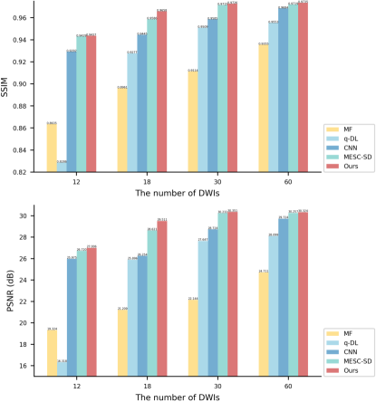
Figure 4: Quantitative evaluation via SSIM and PSNR. The quantitative results were obtained on four different q-space undersampling patterns compared to Model Fitting (MF), q_DL, CNN, and MESC-SD.

4 Results

In this section, we summarize and analyze the experimental results. Then, we conduct an ablation study to investigate the effectiveness of our proposed TDR and NALA.

4.1 Comparison of state-of-the-art methods

4.1.1 Quantitative Evaluation

We evaluate the performance of DeepMpMRI through a comparative analysis with the backbone method and other three state-of-the-art methods. The experimental results are summarized in Table 1, where it can be observed that DeepMpMRI outperforms all other methods in terms of SSIM and PSNR metrics. Specifically, compared to MESC-SD with the same network architecture, DeepMpMRI significantly improves both SSIM and PSNR, demonstrating its effectiveness in simultaneously predicting multiple parameters from various diffusion models.

4.1.2 Qualitative Evaluation

For qualitative analysis, we provide the microstructure estimation results in Fig. 3. The more obvious the structure in the error map, the worse the estimation. As can be seen, the conventional method MF produces significant estimation error and loses anatomical details when sparse sampling is used. The results from Fig. 3 show that the q_DL method yields a relatively low signal-to-noise ratio, while the CNN-based method, although achieving better quantitative results, appears overly smooth in qualitative images, leading to the loss of texture information. We employ MESC-SD as our backbone, which is one of the leading methods for microstructure estimation. When combined with our method, yields improved results. This is evident in the corresponding error maps, which show better preservation of finer details.

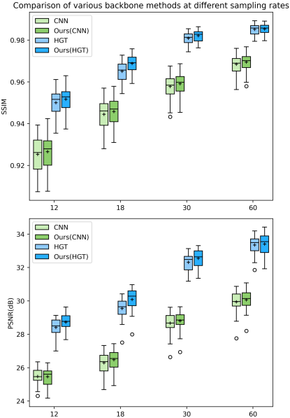
Figure 5: Average microstructure estimation results using different backbone methods (CNN and HGT), in terms of SSIM and PSNR, under different q-space undersampling patterns.

Table 2: The comparison of three variants: backbone, the backbone with TDR, and the proposed DeepMpMRI. The results were obtained with 6 diffusion directions per shell at b-values of 1000, 2000, and 3000 $s/{mm}^{2}$. The best results are in bold.

Methods		SSIM
(18 DWIs)		FA	MD	AD	OD	$V_{ic}$	$V_{iso}$	All
TDR	NALA
×	×	0.9555	0.9665	0.9601	0.9609	0.9654	0.9506	0.9586
✓	×	0.9554	0.9712	0.9639	0.9611	0.9687	0.9600	0.9634
✓	✓	0.9575	0.9724	0.9658	0.9635	0.9722	0.9635	0.9658
Methods		PSNR
(18 DWIs)		FA	MD	AD	OD	$V_{ic}$	$V_{iso}$	All
TDR	NALA
×	×	29.2547	31.1980	30.4241	26.9466	26.7801	28.2336	28.5827
✓	×	29.7238	31.8063	31.0597	26.9941	27.2582	29.9183	29.0857
✓	✓	30.1769	32.0145	31.3210	27.2725	27.9075	30.4814	29.5113

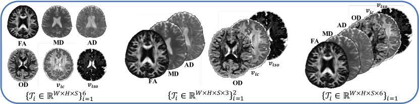
Figure 6: The multi-parameter tensor can be decomposed using three tensor dimensions: decomposing the six parameters separately, combining DTI and NODDI parameters into two groups, and merging all six parameters.

4.2 Comparison of different sampling rates

To further investigate the effectiveness of our method on different sampling rates, three additional q-space undersampling patterns were considered. Consistent with the selection of 18 diffusion gradients, we utilized 12, 30, and 60 diffusion gradients respectively. These gradients consisted of 4, 10, and 20 DWI volumes, acquired along uniform diffusion-decoding directions on each shell with b values of 1000, 2000, and 3000 $s/{mm}^{2}$ using DMRITool [41]. Subsequently, the proposed method and other state-of-the-art techniques were applied to all four cases. Our method achieved high-fidelity microstructure estimation with acceleration factors of 4.5-22.5$\times$ compared to the dense sampling of a total of 270 diffusion gradients. The consistent superior performance of our method across all subsampling patterns was evident from the findings presented in Fig. 4, where the improvement in SSIM and PSNR values confirmed the superiority of DeepMpMRI.

4.3 Ablation Study: Verification of TDR and NALA

We perform an extensive ablation study to investigate the effectiveness of the tensor-decomposition-based regularization (TDR) module and Nesterov-based adaptive learning algorithm (NALA). As shown in Table 2, the ablation study is completed under the condition of a total of 18 gradients (6 diffusion directions per shell at b-values of 1000, 2000, and 3000 $s/{mm}^{2}$). Table 2 shows the quantitative results of the three variants, respectively. According to the quantitative results, the average values of PSNR and SSIM achieved by DeepMpMRI are the highest among the three variants.

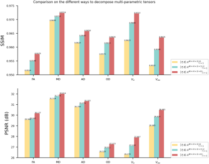
Figure 7: Quantitative comparison of three different decomposition methods based on SSIM and PSNR. The results were obtained with 6 diffusion directions per shell at b-values of 1000, 2000, and 3000 $s/{mm}^{2}$.

5 Discussion

5.1 Discussion on the Different Backbone Methods

As previously mentioned, DeepMpMRI is highly adaptable and can utilize any network architecture as the backbone method when the output is a tensor. The results obtained with various backbone networks are shown in Fig. 5, where we select CNN and HGT for comparison. The results illustrate that regardless of the backbone network used, integrating the proposed DeepMpMRI consistently yields improved results, further validating the effectiveness of the proposed method.

5.2 Discussion on the dimensions of the multi-parameter Tensor

The high dimensionality of multiple parameters allows for various methods to decompose this tensor. This section explores the impact of tensor dimensions on the proposed method. We conducted a detailed study on three tensor dimensions presented in Fig. 6: decomposing the six parameters as individual tensors, grouping the DTI and NODDI parameters into two sets, and merging all six parameters for decomposition. The findings in Fig. 7 suggest that, when considering 18 DWIs (with uniform 6 diffusion directions per shell at b-values of 1000, 2000, and 3000 $s/{mm}^{2}$), the best performance is achieved when merging the six parameters, highlighting the effectiveness of the DeepMpMRI in leveraging the correlations between multiple parameters and the redundancy of high-dimensional data.

6 Conclusion

In this work, we proposed a unified framework, named DeepMpMRI, for simultaneously estimating multiple parametric maps of various diffusion models from sparsely sampled q-space data. In particular, the proposed tensor-decomposition-based regularization can explore shared anatomy and diffusion knowledge among multiple parameters from multiple diffusion models to enhance performance. Since the selection of the weighting hyperparameter is crucial to the performance, we propose a novel Nesterov-based adaptive learning algorithm to dynamically update the hyperparameter, enabling more efficient hyperparameter tuning. We conducted extensive experiments on the HCP dataset at different undersampling patterns. The results demonstrated our model outperforms state-of-the-art methods both quantitatively and qualitatively, obtaining finer-grained results and significantly reducing errors. Compared to the dense sampling of 270 diffusion gradients, our method achieves a high-fidelity microstructure estimation with 4.5-22.5$\times$ acceleration. The proposed framework exhibits excellent flexibility and provides promising guidelines for further research into multi-parametric microstructural imaging.

References

- [1] V. G. Kiselev, “Fundamentals of diffusion MRI physics,” NMR in Biomedicine, vol. 30, no. 3, p. e3602, 2017.
- [2] D. C. Alexander, T. B. Dyrby, M. Nilsson, and H. Zhang, “Imaging brain microstructure with diffusion MRI: practicality and applications,” NMR in Biomedicine, vol. 32, no. 4, p. e3841, 2019.
- [3] M. Camacho, M. Wilms, H. Almgren, K. Amador, R. Camicioli, Z. Ismail, O. Monchi, N. D. Forkert, and A. D. N. Initiative, “Exploiting macro-and micro-structural brain changes for improved parkinson’s disease classification from mri data,” npj Parkinson’s Disease, vol. 10, no. 1, p. 43, 2024.
- [4] S. Soskic, H. F. Tregidgo, E. G. Todd, A. Bouzigues, D. M. Cash, L. L. Russell, D. L. Thomas, I. B. Malone, J. C. van Swieten, L. C. Jiskoot et al., “Dti changes of thalamic subregions in genetic frontotemporal dementia: findings from the genfi cohort,” Alzheimer’s & Dementia, vol. 19, p. e082484, 2023.
- [5] P. J. Basser, J. Mattiello, and D. LeBihan, “MR diffusion tensor spectroscopy and imaging,” Biophysical journal, vol. 66, no. 1, pp. 259–267, 1994.
- [6] D. Le Bihan, J.-F. Mangin, C. Poupon, C. A. Clark, S. Pappata, N. Molko, and H. Chabriat, “Diffusion tensor imaging: concepts and applications,” Journal of Magnetic Resonance Imaging: An Official Journal of the International Society for Magnetic Resonance in Medicine, vol. 13, no. 4, pp. 534–546, 2001.
- [7] K. M. Curran, L. Emsell, and A. Leemans, “Quantitative DTI measures,” Diffusion tensor imaging: A practical handbook, pp. 65–87, 2016.
- [8] K. G. Schilling, D. Archer, F.-C. Yeh, F. Rheault, L. Y. Cai, C. Hansen, Q. Yang, K. Ramdass, A. T. Shafer, S. M. Resnick et al., “Aging and white matter microstructure and macrostructure: a longitudinal multi-site diffusion MRI study of 1218 participants,” Brain Structure and Function, vol. 227, no. 6, pp. 2111–2125, 2022.
- [9] Y. Chen, Y. Wang, Z. Song, Y. Fan, T. Gao, and X. Tang, “Abnormal white matter changes in alzheimer’s disease based on diffusion tensor imaging: A systematic review,” Ageing Research Reviews, p. 101911, 2023.
- [10] X. Chen, N. Roberts, Q. Zheng, Y. Peng, Y. Han, Q. Luo, J. Feng, T. Luo, and Y. Li, “Comparison of diffusion tensor imaging (dti) tissue characterization parameters in white matter tracts of patients with multiple sclerosis (ms) and neuromyelitis optica spectrum disorder (nmosd),” European Radiology, pp. 1–13, 2024.
- [11] Q. Zhu, H. Wang, B. Xu, Z. Zhang, W. Shao, and D. Zhang, “Multimodal triplet attention network for brain disease diagnosis,” IEEE Transactions on Medical Imaging, vol. 41, no. 12, pp. 3884–3894, 2022.
- [12] O. Pasternak, S. Kelly, V. J. Sydnor, and M. E. Shenton, “Advances in microstructural diffusion neuroimaging for psychiatric disorders,” Neuroimage, vol. 182, pp. 259–282, 2018.
- [13] E. Kaden, N. D. Kelm, R. P. Carson, M. D. Does, and D. C. Alexander, “Multi-compartment microscopic diffusion imaging,” NeuroImage, vol. 139, pp. 346–359, 2016.
- [14] M. Caranova, J. F. Soares, S. Batista, M. Castelo-Branco, and J. V. Duarte, “A systematic review of microstructural abnormalities in multiple sclerosis detected with noddi and dti models of diffusion-weighted magnetic resonance imaging,” Magnetic Resonance Imaging, 2023.
- [15] D. Le Bihan, E. Breton, D. Lallemand, P. Grenier, E. Cabanis, and M. Laval-Jeantet, “MR imaging of intravoxel incoherent motions: application to diffusion and perfusion in neurologic disorders.” Radiology, vol. 161, no. 2, pp. 401–407, 1986.
- [16] D. Le Bihan, E. Breton, D. Lallemand, M.-L. Aubin, J. Vignaud, and M. Laval-Jeantet, “Separation of diffusion and perfusion in intravoxel incoherent motion MR imaging.” Radiology, vol. 168, no. 2, pp. 497–505, 1988.
- [17] Y. Assaf, T. Blumenfeld-Katzir, Y. Yovel, and P. J. Basser, “Axcaliber: a method for measuring axon diameter distribution from diffusion MRI,” Magnetic Resonance in Medicine: An Official Journal of the International Society for Magnetic Resonance in Medicine, vol. 59, no. 6, pp. 1347–1354, 2008.
- [18] E. Kaden, F. Kruggel, and D. C. Alexander, “Quantitative mapping of the per-axon diffusion coefficients in brain white matter,” Magnetic resonance in medicine, vol. 75, no. 4, pp. 1752–1763, 2016.
- [19] H. Zhang, T. Schneider, C. A. Wheeler-Kingshott, and D. C. Alexander, “NODDI: practical in vivo neurite orientation dispersion and density imaging of the human brain,” Neuroimage, vol. 61, no. 4, pp. 1000–1016, 2012.
- [20] D. S. Novikov, J. Veraart, I. O. Jelescu, and E. Fieremans, “Rotationally-invariant mapping of scalar and orientational metrics of neuronal microstructure with diffusion MRI,” NeuroImage, vol. 174, pp. 518–538, 2018.
- [21] D. K. Jones, D. C. Alexander, R. Bowtell, M. Cercignani, F. Dell’Acqua, D. J. McHugh, K. L. Miller, M. Palombo, G. J. Parker, U. S. Rudrapatna et al., “Microstructural imaging of the human brain with a ‘super-scanner’: 10 key advantages of ultra-strong gradients for diffusion MRI,” NeuroImage, vol. 182, pp. 8–38, 2018.
- [22] E. T. McKinnon, J. A. Helpern, and J. H. Jensen, “Modeling white matter microstructure with fiber ball imaging,” Neuroimage, vol. 176, pp. 11–21, 2018.
- [23] D. Le Bihan, C. Poupon, A. Amadon, and F. Lethimonnier, “Artifacts and pitfalls in diffusion MRI,” Journal of Magnetic Resonance Imaging: An Official Journal of the International Society for Magnetic Resonance in Medicine, vol. 24, no. 3, pp. 478–488, 2006.
- [24] V. Golkov, A. Dosovitskiy, J. I. Sperl, M. I. Menzel, M. Czisch, P. Sämann, T. Brox, and D. Cremers, “Q-space deep learning: twelve-fold shorter and model-free diffusion MRI scans,” IEEE transactions on medical imaging, vol. 35, no. 5, pp. 1344–1351, 2016.
- [25] E. K. Gibbons, K. K. Hodgson, A. S. Chaudhari, L. G. Richards, J. J. Majersik, G. Adluru, and E. V. DiBella, “Simultaneous NODDI and GFA parameter map generation from subsampled q-space imaging using deep learning,” Magnetic resonance in medicine, vol. 81, no. 4, pp. 2399–2411, 2019.
- [26] Q. Tian, B. Bilgic, Q. Fan, C. Liao, C. Ngamsombat, Y. Hu, T. Witzel, K. Setsompop, J. R. Polimeni, and S. Y. Huang, “DeepDTI: High-fidelity six-direction diffusion tensor imaging using deep learning,” NeuroImage, vol. 219, p. 117017, 2020.
- [27] H. Li, Z. Liang, C. Zhang, R. Liu, J. Li, W. Zhang, D. Liang, B. Shen, X. Zhang, Y. Ge et al., “SuperDTI: Ultrafast DTI and fiber tractography with deep learning,” Magnetic resonance in medicine, vol. 86, no. 6, pp. 3334–3347, 2021.
- [28] A. Daducci, E. J. Canales-Rodríguez, H. Zhang, T. B. Dyrby, D. C. Alexander, and J.-P. Thiran, “Accelerated microstructure imaging via convex optimization (AMICO) from diffusion MRI data,” Neuroimage, vol. 105, pp. 32–44, 2015.
- [29] C. Ye, X. Li, and J. Chen, “A deep network for tissue microstructure estimation using modified LSTM units,” Medical image analysis, vol. 55, pp. 49–64, 2019.
- [30] C. Ye, Y. Li, and X. Zeng, “An improved deep network for tissue microstructure estimation with uncertainty quantification,” Medical image analysis, vol. 61, p. 101650, 2020.
- [31] G. Chen, Y. Hong, Y. Zhang, J. Kim, K. M. Huynh, J. Ma, W. Lin, D. Shen, P.-T. Yap, and U. B. C. P. Consortium, “Estimating tissue microstructure with undersampled diffusion data via graph convolutional neural networks,” in International Conference on Medical Image Computing and Computer-Assisted Intervention. Springer, 2020, pp. 280–290.
- [32] G. Chen, H. Jiang, J. Liu, J. Ma, H. Cui, Y. Xia, and P.-T. Yap, “Hybrid graph transformer for tissue microstructure estimation with undersampled diffusion MRI data,” in International Conference on Medical Image Computing and Computer-Assisted Intervention. Springer, 2022, pp. 113–122.
- [33] Q. Fan, Q. Tian, C. Ngamsombat, and S. Y. Huang, “DeepHIBRID: How to condense the sampling in the kq joint space for microstructural diffusion metric estimation empowered by deep learning,” in Proceedings of International Society for Magnetic Resonance in Medicine, 2020, p. 4405.
- [34] J. Park, W. Jung, E.-J. Choi, S.-H. Oh, J. Jang, D. Shin, H. An, and J. Lee, “DIFFnet: diffusion parameter mapping network generalized for input diffusion gradient schemes and b-value,” IEEE Transactions on Medical Imaging, vol. 41, no. 2, pp. 491–499, 2021.
- [35] S. HashemizadehKolowri, R.-R. Chen, G. Adluru, and E. V. DiBella, “Jointly estimating parametric maps of multiple diffusion models from undersampled q-space data: A comparison of three deep learning approaches,” Magnetic Resonance in Medicine, vol. 87, no. 6, pp. 2957–2971, 2022.
- [36] T. G. Kolda, “Orthogonal tensor decompositions,” SIAM Journal on Matrix Analysis and Applications, vol. 23, no. 1, pp. 243–255, 2001.
- [37] T. G. Kolda and B. W. Bader, “Tensor decompositions and applications,” SIAM review, vol. 51, no. 3, pp. 455–500, 2009.
- [38] J. Chen and Y. Saad, “On the tensor svd and the optimal low rank orthogonal approximation of tensors,” SIAM journal on Matrix Analysis and Applications, vol. 30, no. 4, pp. 1709–1734, 2009.
- [39] Y. Nesterov, “A method for solving the convex programming problem with convergence rate O(1/k2),” Proceedings of the USSR Academy of Sciences, vol. 269, pp. 543–547, 1983.
- [40] J. Cheng, D. Shen, P.-T. Yap, and P. J. Basser, “Novel single and multiple shell uniform sampling schemes for diffusion MRI using spherical codes,” in Medical Image Computing and Computer-Assisted Intervention–MICCAI 2015: 18th International Conference, Munich, Germany, October 5-9, 2015, Proceedings, Part I 18. Springer, 2015, pp. 28–36.
- [41] J. Cheng, D. Shen, P. Yap, and P. J. Basser, “Single-and multiple-shell uniform sampling schemes for diffusion MRI using spherical codes,” IEEE transactions on medical imaging, vol. 37, no. 1, pp. 185–199, 2017.
- [42] M. E. Kilmer and C. D. Martin, “Factorization strategies for third-order tensors,” Linear Algebra and its Applications, vol. 435, no. 3, pp. 641–658, 2011.
- [43] M. E. Kilmer, L. Horesh, H. Avron, and E. Newman, “Tensor-tensor algebra for optimal representation and compression of multiway data,” Proceedings of the National Academy of Sciences, vol. 118, no. 28, p. e2015851118, 2021.
- [44] F. L. Hitchcock, “The expression of a tensor or a polyadic as a sum of products,” Journal of Mathematics and Physics, vol. 6, no. 1-4, pp. 164–189, 1927.
- [45] R. A. Harshman et al., “Foundations of the parafac procedure: Models and conditions for an “explanatory” multi-modal factor analysis,” UCLA working papers in phonetics, vol. 16, no. 1, p. 84, 1970.
- [46] L. R. Tucker, “Implications of factor analysis of three-way matrices for measurement of change,” Problems in measuring change, vol. 15, no. 122-137, p. 3, 1963.
- [47] L. De Lathauwer, B. De Moor, and J. Vandewalle, “A multilinear singular value decomposition,” SIAM journal on Matrix Analysis and Applications, vol. 21, no. 4, pp. 1253–1278, 2000.
- [48] I. V. Oseledets, “Tensor-train decomposition,” SIAM Journal on Scientific Computing, vol. 33, no. 5, pp. 2295–2317, 2011.
- [49] I. O. Jelescu, J. Veraart, E. Fieremans, and D. S. Novikov, “Degeneracy in model parameter estimation for multi-compartmental diffusion in neuronal tissue,” NMR in Biomedicine, vol. 29, no. 1, pp. 33–47, 2016.
- [50] D. S. Novikov, V. G. Kiselev, and S. N. Jespersen, “On modeling,” Magnetic resonance in medicine, vol. 79, no. 6, pp. 3172–3193, 2018.
- [51] I. O. Jelescu, M. Palombo, F. Bagnato, and K. G. Schilling, “Challenges for biophysical modeling of microstructure,” Journal of Neuroscience Methods, vol. 344, p. 108861, 2020.
- [52] J. Cheng, D. Shen, P. J. Basser, and P.-T. Yap, “Joint 6d k-q space compressed sensing for accelerated high angular resolution diffusion MRI,” in International Conference on Information Processing in Medical Imaging. Springer, 2015, pp. 782–793.
- [53] P.-T. Yap, Y. Zhang, and D. Shen, “Multi-tissue decomposition of diffusion MRI signals via sparse-group estimation,” IEEE Transactions on Image Processing, vol. 25, no. 9, pp. 4340–4353, 2016.
- [54] E. Schwab, R. Vidal, and N. Charon, “Joint spatial-angular sparse coding for dMRI with separable dictionaries,” Medical image analysis, vol. 48, pp. 25–42, 2018.
- [55] E. Schwab, B. D. Haeffele, R. Vidal, and N. Charon, “Global optimality in separable dictionary learning with applications to the analysis of diffusion MRI,” SIAM Journal on Imaging Sciences, vol. 12, no. 4, pp. 1967–2008, 2019.
- [56] F. Shi, J. Cheng, L. Wang, P.-T. Yap, and D. Shen, “Super-resolution reconstruction of diffusion-weighted images using 4d low-rank and total variation,” in Computational Diffusion MRI: MICCAI Workshop, Munich, Germany, October 9th, 2015. Springer, 2016, pp. 15–25.
- [57] C. Zhang, T. M. Arefin, U. Nakarmi, C. H. Lee, H. Li, D. Liang, J. Zhang, and L. Ying, “Acceleration of three-dimensional diffusion magnetic resonance imaging using a kernel low-rank compressed sensing method,” Neuroimage, vol. 210, p. 116584, 2020.
- [58] G. Ramos-Llordén, G. Vegas-Sánchez-Ferrero, C. Liao, C.-F. Westin, K. Setsompop, and Y. Rathi, “Snr-enhanced diffusion MRI with structure-preserving low-rank denoising in reproducing kernel hilbert spaces,” Magnetic resonance in medicine, vol. 86, no. 3, pp. 1614–1632, 2021.
- [59] R. W. Liu, L. Shi, W. Huang, J. Xu, S. C. H. Yu, and D. Wang, “Generalized total variation-based MRI rician denoising model with spatially adaptive regularization parameters,” Magnetic resonance imaging, vol. 32, no. 6, pp. 702–720, 2014.
- [60] I. Teh, D. McClymont, E. Carruth, J. Omens, A. McCulloch, and J. E. Schneider, “Improved compressed sensing and super-resolution of cardiac diffusion MRI with structure-guided total variation,” Magnetic resonance in medicine, vol. 84, no. 4, pp. 1868–1880, 2020.
- [61] C. Eckart and G. Young, “The approximation of one matrix by another of lower rank,” Psychometrika, vol. 1, no. 3, pp. 211–218, 1936.
- [62] J. D. Carroll and J.-J. Chang, “Analysis of individual differences in multidimensional scaling via an n-way generalization of “eckart-young” decomposition,” Psychometrika, vol. 35, no. 3, pp. 283–319, 1970.
- [63] J. Bergstra and Y. Bengio, “Random search for hyper-parameter optimization.” Journal of machine learning research, vol. 13, no. 2, 2012.
- [64] A. G. Baydin, R. Cornish, D. M. Rubio, M. Schmidt, and F. Wood, “Online learning rate adaptation with hypergradient descent,” arXiv preprint arXiv:1703.04782, 2017.
- [65] L. B. Almeida, T. Langlois, J. D. Amaral, and A. Plakhov, “Parameter adaptation in stochastic optimization,” in On-line learning in neural networks, 1999, pp. 111–134.
- [66] D. M. Rubio, “Convergence analysis of an adaptive method of gradient descent,” University of Oxford, Oxford, M. Sc. thesis, 2017.
- [67] J. T. Zhou, K. Di, J. Du, X. Peng, H. Yang, S. J. Pan, I. Tsang, Y. Liu, Z. Qin, and R. S. M. Goh, “Sc2net: Sparse lstms for sparse coding,” in Proceedings of the AAAI Conference on Artificial Intelligence, vol. 32, no. 1, 2018.
- [68] D. C. Van Essen, S. M. Smith, D. M. Barch, T. E. Behrens, E. Yacoub, K. Ugurbil, W.-M. H. Consortium et al., “The WU-Minn human connectome project: an overview,” Neuroimage, vol. 80, pp. 62–79, 2013.
- [69] G. Chen, Y. Hong, K. M. Huynh, and P.-T. Yap, “Deep learning prediction of diffusion MRI data with microstructure-sensitive loss functions,” Medical image analysis, vol. 85, p. 102742, 2023.