Primordial power spectrum at N3LO in effective theories of inflation

Abstract

We develop a systematic framework to compute the primordial power spectrum up to next-to-next-to-next to leading order (N3LO) in the Hubble-flow parameters for a large class of effective theories of inflation. We assume that the quadratic action for perturbations is characterized by two functions of time—the kinetic amplitude and the speed of sound—that are independent of the Fourier mode $k$. Using the Green’s function method introduced by Stewart & Gong and developed by Auclair & Ringeval, we determine the primordial power spectrum, including its amplitude, spectral indices, their running and running of their running, starting from a given generic action for perturbations. As a check, we reproduce the state-of-the-art results for scalar and the tensor power spectrum of the simplest “vanilla” models of single-field inflation. The framework applies to Weinberg’s effective field theory of inflation (with the condition of no parity violation) and to effective theory of spontaneous de Sitter-symmetry breaking. As a concrete application, we provide the expression for the N3LO power spectrum of $R+R^{2}$ Starobinsky inflation, without a field redefinition. All expressions are provided in terms of an expansion in one single parameter, the number of inflationary e-foldings $N_{\ast}$. Surprisingly we find that, compared to previous leading-order calculations, for $N_{\ast}=55$ the N3LO correction results in a $7\%$ decrease of the predicted tensor-to-scalar ratio, in addition to a deviation from the consistency relation. These results provide precise theoretical predictions for the next generation of CMB observations.

I Introduction

Cosmic inflation [1, 2, 3, 4, 5, 6, 7, 8, 9, 10] provides a mechanism for the production of primordial perturbations that is successful in explaining a wide range of cosmological observations, including the nature of anisotropies in the temperature fluctuations of the cosmic microwave background (CMB), and the quantum origin of the large scale structure of the Universe [11, 12]. Within this theoretical framework, there is a plethora of inflationary models which range from quantum-gravity motivated models to phenomenological parametrizations of potentials [13], and additional observations are required to distinguish between different models. Thus, as upcoming cosmological observations are expected to improve the constraints on many of the primordial observables [14, 15, 16], precise theoretical predictions for these future observations are also required. We address this issue directly for the large class of inflationary models summarized in Tab. 1.

The primordial power spectrum is one of the most relevant cosmological observables. The Green’s function method introduced by Stewart and Gong in [17] was recently extended by Auclair and Ringeval [18] to provide a detailed computation of the next-to-next-to-next to leading order (N3LO) power spectrum in the framework of single-field slow-roll inflation—a phase driven by a minimally-coupled scalar field slowly rolling down its potential—together with an extension to non-minimal kinetic terms obtained via a mapping method [19]. These models belong to a broader class of effective theories of inflation that we discuss here. The prototypical example is the action for the free propagation of scalar curvature perturbations $\mathcal{R}$,

$$S_{2}[\mathcal{R}]=\frac{1}{2}\int\!\differential[4]{x}a(t)^{3}\,Z_{\textrm{s}}(t)\Big{(}\dot{\mathcal{R}}^{2}-\frac{c_{\textrm{s}}(t)^{2}}{a(t)^{2}}(\partial_{i}\mathcal{R})^{2}\Big{)}\,,$$ (1)

where the non-trivial time-dependence of the background fields and geometry, assumed to be homogeneous and isotropic, is encoded in three functions of time—the scale factor $a(t)$, the kinetic amplitude $Z_{s}(t)$ and the speed of sound $c_{s}(t)$ [20]. While in a given model these functions take a specific form, it is useful to treat them as independent to obtain general formulas which apply to all perturbations in a scalar-vector-tensor decomposition. We work in a spatially-flat quasi-de Sitter background and assume that there is no gravitational parity violation, which implies that the functions $Z_{s}(t)$ and $c_{s}(t)$ admit a Hubble-flow expansion and are independent of the mode $k$ in Fourier space. The goal of this paper is to provide a N3LO computation of the primordial power spectrum and its features (amplitude, tilt, running and running-of-the-running) for the broad family of effective theories of inflation (Tab. 1) which have quadratic action of this form.

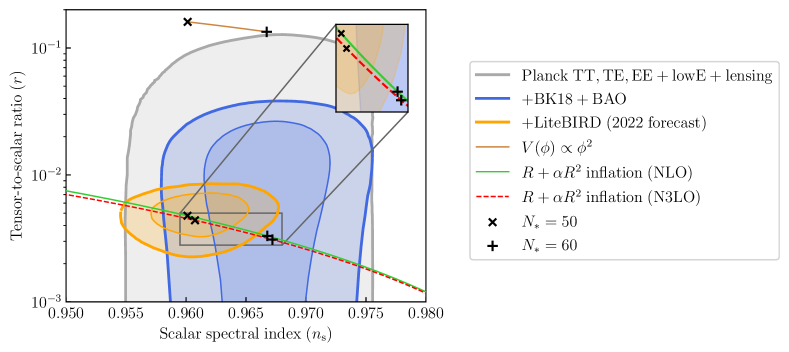
Figure 1: Marginalized joint 68% and 95% C.L. regions for $n_{\mathrm{s}}$ and $r$ at $k_{\ast}=0.002$ Mpc^-1 as reported by the Planck Collaboration [11], and the BICEP2/Keck Collaboration [21]. The orange region represents the forecast of the upcoming LiteBIRD experiment for a fiducial model with $r=0.005$ [16]. Our results for Starobinsky inflation up to N3LO are shown in the dashed red line. We note the a $7\%$ decrease for $r$ and a $0.05\%$ increase for $n_{\mathrm{s}}$ with respect to the standard NLO expressions, for $N_{\ast}=55$.

Table 1: Effective models of inflation. The functions $Z(t)$ and $c(t)$ are defined by the quadratic action for scalar ($\mathrm{s}$) and tensor ($\mathrm{t}$) perturbations of the form (4). The symbols indicate that the functions reported are of the form considered here (✓) or not ($\times$). A symbol “$\dagger$” indicates that the effective theory requires an additional assumption of no parity violation to exclude a dependence on $k$ in the functions $Z(t)$ and $c(t)$.

Theory	$Z_{\mathrm{s}}(t)$	$c_{\textrm{s}}(t)$	$Z_{\mathrm{t}}(t)$	$c_{\textrm{t}}(t)$
Single-field [22]	Eq. (74)	$1$	Eq. (75)	$1$
$R+\alpha R^{2}$ [23]	Eq. (96)	$1$	Eq. (99)	$1$
$K$-inflation [24]	✓	✓	✓	$1$
LQC+inflaton [25, 26]	✓	✓	✓	✓
$f(\varphi)$-Gauss Bonnet [27]	✓	✓	✓	✓
$f(\varphi)$-Chern Simons [28, 29]	✓	✓	$\times$	$\times$
General scalar-tensor [23]	✓	✓	✓	✓
Goldston mode EFT [20]	✓	✓	✓	✓
Multifield EFT [30]	✓	✓	✓	✓
Minimally broken CFT [31]	✓	✓	$\checked\dagger$	$\checked\dagger$
Weinberg’s EFT [32]	✓	✓	$\checked\dagger$	$\checked\dagger$

In an exactly de Sitter background, the Mukhanov-Sasaki equation admits an exact solution for the mode functions which corresponds to the choice of Bunch-Davies vacuum for the quantum perturbations. The constant Hubble rate $H(t)=H_{\ast}$ results in a scale-invariant power spectrum $P\sim H_{\ast}^{2}$. This leading order (LO) prediction is corrected by a next-to-leading order contribution (NLO) that takes into account the fact that the Hubble rate $H(t)$ decreases slowly, imprinting more power in red than in blue modes—a red tilt $n_{s}\lesssim 1$. At this order, the approximate equation admits again an exact solution which defines a quasi-Bunch-Davies vacuum with mode functions given by a combination of Bessel functions [33]. However, the solution in terms of Bessel functions is not easily extended to higher orders, and various approximation schemes have been developed, including the uniform approximation [34, 35, 36, 37, 38, 39, 40]. The next-to-next-to-leading order (N2LO) corrections for scalar perturbations were derived in [41] using the constant-horizon approximation, and in [17], as a systematic expansion using the Green’s function method, while the N2LO corrections to tensor modes was obtained in [42]. The fully expanded N3LO corrections for slow-roll inflation was derived in [18], which is the method we adopt and extend here. Motivated by these recent results, we address the problem of finding the contributions to the power spectrum up to N3LO for the broad class of models with perturbations described by the quadratic action (4). In particular we work out the N3LO predictions of the model of inflation introduced by Starobinsky in 1979, motivated by quantum gravity considerations [2, 3]. Remarkably, this model provides the best account of current observations in terms of a single free parameter, the number of inflationary e-foldings $N_{\ast}$. While its analysis is generally done via a field redefinition that maps it into an inflaton potential (Einstein frame), here we work in the geometric framework where inflation is driven by higher curvature terms (Jordan frame). We note that the minimal coupling of matter to Starobinsky inflation in the geometric framework induces a slightly different reheating history and future observations that include reheating constraints are expected to distinguish the two scenarios [12]. In Fig. 1 we show that the N3LO correction computed here decreases the standard prediction of the tensor-to-scalar ratio by $7\%$.

The manuscript is structured as follows: In Sec. II we describe the assumptions, the general framework and the Hubble-flow expansion of the background variables. In Sec. III we discuss the quantization of perturbations, a choice of variables analogous to Mukhanov-Sasaki variables, and a logarithmic expansion of the Hubble-flow parameters. In Sec. IV we find the mode equation satisfied by our dynamical variables and describe the Green’s function method introduced in [17, 18]. In Sec. V we report the final expressions for the power spectrum, which takes the schematic form,

$$\mathcal{P}_{0}^{(\psi)}(k)=\frac{\hbar H_{\ast}^{2}}{4\pi^{2}c_{\ast}^{3}Z_{\ast}}\left[1+p_{1}(k)+p_{2}(k)+p_{3}(k)\right],$$ (2)

with $H$, $Z$ and $c$ evaluated at the pivot scale $k_{\ast}$. The functions $p_{n}(k)$ have a logarithmic dependence, i.e., include powers of $\ln(k/k_{\ast})$, and represent the N$n$LO correction to the power spectrum. From this expression, we extract the predictions for the amplitude, tilt, running of the tilt, and running-of-the-running of the tilt, which are reported in Tab. 2 and 3. In Sec. VI we fully reproduce the state-of-the-art N3LO corrections for single field inflation, reported in Tab. 4 and 5. In Sec. VII we analyze Starobinsky inflation and compute the N3LO corrections as an expansion in the single parameter $N_{\ast}$, reported in Tab. 6. Finally, in Sec. VIII we discuss the results obtained in this work and outline possible extensions.

Throughout the paper we adopt units with speed of light $\mathrm{c}=1$, while we keep track of Planck’s constant $\hbar$ and Newton’s gravitational constant $G$. The metric signature is $(-+++)$, a derivative with respect to cosmic time is denoted by a dot $(\dot{\phantom{a}})$, and a derivative with respect to other variables by a prime $(\phantom{1})^{\prime}$. Complex conjugation is denoted by $(\phantom{1})^{\ast}$, and evaluation at the pivot scale by $(\phantom{1})_{\ast}$.

II Action and perturbations

Quadratic action

We consider an inflationary background geometry given by the spatially-flat Friedman-Lemaître-Robertson-Walker (FLRW) metric

$$\bar{g}_{\mu\nu}\differential{x}^{\mu}\differential{x}^{\nu}=-\differential{t}^{2}+a(t)^{2}\,\delta_{ij}\differential{x}^{i}\differential{x}^{j}\,,$$ (3)

which, together with other homogeneous and isotropic fields, satisfies the background equations of motion of an inflationary theory of gravity and matter. Because of the symmetry of the background, perturbations of the geometry and of matter fields decompose in scalar, vector and tensor modes (SVT). Once one fixes a gauge and solves the Hamiltonian & diffeomorphism constraints perturbatively, the action of perturbations decouples at quadratic order and takes the general form

$$S_{2}[\psi]=\int\differential{t}\int\frac{\differential[3]{\mathbf{k}}}{(2\pi)^{3}}\,a(t)^{3}Z_{\psi}(t)\left[\frac{1}{2}\big{|}\dot{\psi}(\mathbf{k},t)\big{|}^{2}-\frac{1}{2}c_{\psi}(t)^{2}\,\frac{k^{2}}{a(t)^{2}}\absolutevalue{\psi(\mathbf{k},t)}^{2}\right],$$ (4)

where $k=\absolutevalue{\mathbf{k}}$ and we used the generic name $\psi(\mathbf{k},t)$ for the Fourier transform of each of the SVT modes $\Psi(\mathbf{x},t)$,

$$\Psi(\mathbf{x},t)=\int\frac{\differential[3]{\mathbf{k}}}{(2\pi)^{3}}\,\psi(\mathbf{k},t)\,\mathrm{e}^{\mathrm{i}\mathbf{k}\cdot\mathbf{x}}.$$ (5)

Together with the scale factor $a(t)$, the quadratic action encodes the coupling of the SVT modes to the background via two functions of time $t$: The kinetic amplitude, $Z_{\psi}(t)$, and the speed of sound, $c_{\psi}(t)$. In a given model, their time dependence can be expressed in terms of time-derivatives of the Hubble rate $H(t)=\dot{a}(t)/a(t)$, but here we treat them as independent as it allows us to derive general results. We make the assumption that they do not depend on the mode $k$ (which excludes some models of inflation), and require both a no-ghost condition, $Z_{\psi}(t)>0$, and no-Laplacian-instability condition, $c_{\psi}(t)^{2}>0$.

The well-studied case of single-field inflation corresponds to the two functions being constant for tensor modes, while scalar curvature perturbations have a constant speed of sound and a time-dependent kinetic amplitude $Z_{s}(t)$ proportional to the slow-roll parameter $-\dot{H}(t)/H(t)^{2}$. In the case of Starobinsky inflation treated in the geometric framework, $Z_{\mathrm{s}}(t)$ and $Z_{\mathrm{t}}(t)$ depend non-trivially on higher time-derivative of the Hubble rate both for scalar and for tensor modes, but the speed of sound is still constant for both.

The effective field theory of single-field [20] and multi-field [30] inflation has a quadratic action of this form, with a non-trivial speed of sound $c_{\psi}(t)$ that needs to be determined via observations, and a non-trivial kinetic amplitude $Z_{\psi}(t)$ that depends on the slow-roll parameter and on the speed of sound.

In loop quantum cosmology, quantum geometry effects modify the Mukhanov-Sasaki equation which, in a self-consistent approximation, can also be cast in the form (4), [25, 26].

In models of $K$-inflation [24], the action of the inflaton field includes higher derivative terms of the form

$$S_{K\mathrm{infl}}=\int\!\differential[4]{x}\sqrt{-g}\,f_{K}(\varphi)\,\big{(}g^{\mu\nu}\partial_{\mu}\varphi\partial_{\nu}\varphi\big{)}^{2}\,,$$ (6)

which result again in an action for scalar perturbations of the form (4) with a non-trivial speed of sound. Similarly, models that include a coupling $f_{GB}(\varphi)\mathcal{L}_{GB}$ to the Gauss-Bonnet density [27],

$$\mathcal{L}_{GB}=R_{\mu\nu\rho\sigma}R^{\mu\nu\rho\sigma}\!-\!4R_{\mu\nu}R^{\mu\nu}\!+\!R^{2}\,,$$ (7)

can be cast in the form (4) for scalar pertubations. On the other hand, in models with a coupling $f_{CS}(\varphi)\mathcal{L}_{CS}$ to the Chern-Simons density,

$$\mathcal{L}_{CS}=-(\sqrt{-g})^{-1}\,\epsilon^{\mu\nu\rho\sigma}\,R^{\alpha}{}_{\beta\mu\nu}\,R^{\beta}{}_{\alpha\rho\sigma}\,,$$ (8)

tensor perturbations with circular polarization $(\pm)$ have a kinetic term $Z_{\pm}(t,k)$ and speed of sound $c_{\pm}(t,k)$ which depend linearly on $\pm k$, resulting in gravitational parity violation [28, 29]. Therefore they cannot be cast in the form (4) assumed here because of the dependence on $k$.

Weinberg’s formulation of an effective field theory of single-field inflation starts from the most general action $S[g_{\mu\nu},\varphi]$ which includes all diffeomorphism invariant terms, organized in an order-by-order expansion in the number of spacetime derivatives, up to fourth order [32]. In particular, it includes a coupling of the inflaton field $\varphi$ to terms quadratic in the Weyl tensor, $C_{\mu\nu\rho\sigma}C^{\mu\nu\rho\sigma}$ and $(\sqrt{-g})^{-1}\epsilon^{\mu\nu\rho\sigma}\,C^{\alpha}{}_{\beta\mu\nu}\,C^{\beta}{}_{\alpha\rho\sigma}$, and a term of the $K$-inflation type (6). Up to field redefinitions, and using reduction of order of the four-derivative terms with respect to the (two-derivative) Einstein equations of motion

$$R_{\mu\nu}=8\pi G\;(T_{\mu\nu}-\tfrac{1}{2}g_{\mu\nu}T)\,,$$ (9)

one can reabsorb terms quadratic in the Ricci tensor into a $K$-inflation term. Therefore, the effective action takes the form of single-field inflation with an inflaton potential $V(\varphi)$, a $K$-inflation term (6), a $GB$-coupling (7) and a $CS$-coupling (8). If we further assume that the theory is invariant under all diffeomorphisms, including diffeomorphisms not connected with the identity such as orientation reversals, then the parity-violating coupling to $\mathcal{L}_{CS}$ has to vanish, and the quadratic action for scalar and tensor perturbation takes once more the form (4), with the kinetic amplitude and the speed of sound expressed in terms of time-derivatives of the Hubble rate $H(t)$, of the background inflaton field $\bar{\varphi}(t)$, and of the couplings $V(\bar{\varphi}(t))$, $f_{K}(\bar{\varphi}(t))$ and $f_{GB}(\bar{\varphi}(t))$.

The formalism that we develop here applies to this broad class of effective theories of inflation (Tab. 1).

Hubble-flow expansion

The variational principle for the quadratic action (4) results in equations of motion for the SVT perturbations that depend on the background functions $a(t)$, $H(t)$, $Z_{\psi}(t)$, $c_{\psi}(t)$ and their time derivatives. In the simplest models, the mechanism that produces a frozen power spectrum for tensor modes is a transition in the mode equation $\ddot{u}(t)+3H(t)\,\dot{u}(t)+(k/a(t))^{2}\,u(t)=0$ from an oscillatory phase with small friction $H(t)\ll k/a(t)$, to an overdamped phase with large friction $H(t)\gg k/a(t)$. For a given mode $k$, the transition requires an increasing comovind scale $a(t)H(t)$, i.e., an accelerating phase

$$0<\ddot{a}=\derivative{t}\,\big{(}a(t)H(t)\big{)}=\big{(}1-\epsilon_{1H}(t)\big{)}\,a(t)H(t)^{2}\,,$$ (10)

or equivalently a Hubble-flow parameter $\epsilon_{1H}(t)<1$ with

$$\epsilon_{1H}(t)\equiv-\frac{\dot{H}(t)}{H(t)^{2}}\,.$$ (11)

During a de Sitter phase, $a_{0}(t)=\mathrm{e}^{H_{0}t}$, the Hubble rate is constant and therefore the Hubble-flow parameter vanishes exactly. In a quasi-de Sitter phase, the Hubble rate is assumed to change slowly and it is useful to introduce a systematic expansion, called Hubble-flow expansion [41], defined recursively in terms of the dimensionless parameters $\epsilon_{nH}$, with

$$\epsilon_{(n+1)H}(t)\equiv-\frac{\dot{\epsilon}_{nH}(t)}{H(t)\,\epsilon_{nH}(t)}\,.$$ (12)

A phase of quasi-de Sitter inflation is characterized by $\absolutevalue{\epsilon_{nH}}\ll 1$. Similarly, we introduce new Hubble-flow parameters for the kinetic amplitude $Z_{\psi}(t)$,

$$\epsilon_{1Z}(t)\, \equiv-\frac{\dot{Z}_{\psi}(t)}{H(t)Z_{\psi}(t)}\,,$$ (13)

$$\epsilon_{(n+1)Z}(t)\, \equiv-\frac{\dot{\epsilon}_{nZ}(t)}{H(t)\,\epsilon_{nZ}(t)}\,,$$ (14)

and for the speed of sound $c_{\psi}(t)$,

$$\epsilon_{1c}(t)\, \equiv-\frac{\dot{c}_{\psi}(t)}{H(t)c_{\psi}(t)}\,,$$ (16)

$$\epsilon_{(n+1)c}(t)\, \equiv-\frac{\dot{\epsilon}_{nc}(t)}{H(t)\,\epsilon_{nc}(t)}\,.$$ (17)

All the flow parameter are assumed to be of the same order, e.g., $\order{\epsilon_{nH}}=\order{\epsilon_{n^{\prime}Z}}=\order{\epsilon_{n^{\prime\prime}c}}$. To simplify the notation, we use a placeholder $\epsilon$ to track the corresponding order of the expansion, i.e., $\order{\epsilon_{1H}}=\order{\epsilon}$, $\order{\epsilon_{1Z}^{2}}=\order{\epsilon^{2}}$ and so on. In a specific model of inflation, this assumption is to be checked a posteriori. In this work we consider corrections up to order $\epsilon^{3}$.

III Quantization of perturbations

Field representation and mode expansion

Inflation explains the anisotropies in the CMB temperature and the seeds of large-scale structures in terms of vacuum fluctuations that are assumed to be homogeoneous and isotropic. Specifically, the SVT fields $\hat{\Psi}(\mathbf{x},t)$ are assumed to be initially in a vacuum state $|0\rangle$ with a two-point correlation function that, at equal time $t$, is invariant under rotations and translations,

$$\bra{0}\hat{\Psi}(\mathbf{x},t)\hat{\Psi}(\mathbf{x}^{\prime},t)\ket{0}\;=\;G\big{(}|\mathbf{x}-\mathbf{x}^{\prime}|,t\big{)}\,.$$ (18)

Neglecting interactions and non-Gaussianities, this condition can be encoded in a Gaussian vacuum state in Fock space, defined by the condition $\hat{a}(\mathbf{k})\ket{0}=0\,,\;\forall\mathbf{k}$, with bosonic creation and annihilation operators, $[\hat{a}(\mathbf{k}),\hat{a}^{\dagger}(\mathbf{k^{\prime}}))]=(2\pi)^{3}\delta^{(3)}(\mathbf{k}+\mathbf{k}^{\prime})$, together with a mode expansion of the quantum field

$$\hat{\Psi}(\mathbf{x},t)=\!\int\!\frac{\differential[3]{\mathbf{k}}}{(2\pi)^{3}}\left(u(k,t)\hat{a}(\mathbf{k})+u^{\ast}(k,t)\hat{a}^{\dagger}(\mathbf{k})\right)\mathrm{e}^{i\mathbf{k}\cdot\mathbf{x}}.$$ (19)

The assumption of homogeneity and isotropy (18) implies that the modes $u(k,t)$ depend only on $k=|\mathbf{k}|$. Moreover, at the classical level, the conjugate momentum derived from the action (4) is defined by

$$\pi(\mathbf{k},t)\equiv\functionalderivative{S_{2}[\psi]}{\dot{\psi}(\mathbf{k},t)}=\frac{a(t)^{3}Z_{\psi}(t)}{(2\pi)^{3}}\dot{\psi}(-\mathbf{k},t)\,,$$ (20)

and denoted $\Pi(\mathbf{x},t)$ in position space. Canonical quantization of the Poisson brackets results in the canonical commutation relation (CCR), $[\hat{\Psi}(\mathbf{x},t),\hat{\Pi}(\mathbf{x}^{\prime},t)]=\mathrm{i}\,\hbar\,\delta^{(3)}(\mathbf{x}-\mathbf{x}^{\prime})$ which, together with (19), implies the canonical Wronskian condition for the mode functions

$$u(k,t)\dot{u}^{\ast}(k,t)-\dot{u}(k,t)u^{\ast}(k,t)=\frac{\mathrm{i}\,\hbar}{a(t)^{3}\,Z_{\psi}(t)},$$ (21)

where $u^{\ast}$ is the complex conjugate of $u$. Finally, the equations of motion (EoM) derived from the action (4) for each of the SVT modes results in the mode equation

$$\ddot{u}(k,t)+(3-\epsilon_{Z1}(t))H(t)\dot{u}(k,t)+c_{\psi}(t)^{2}\frac{k^{2}}{a(t)^{2}}\,u(k,t)=0\,.$$ (22)

A choice of initial conditions $u(k,t_{0}),\dot{u}(k,t_{0})$ for the EoM (22), satisfying the CCR constraint (21), or equivalently a choice of solution of the two equations, defines a Gaussian state $|0\rangle$ that is homogeneous and isotropic, (18). In the next section we discuss how to select an adiabatic solution of (22)–(21) that generalizes the Bunch-Davies vacuum to quasi-de Sitter space, order by order in the Hubble-flow expansion.

Mukhanov-Sasaki variables

In de Sitter space the Hubble rate is constant, $a_{0}(t)=\mathrm{e}^{H_{0}t}$, and in the simplest models of a test quantum field, the EoM reduces to $\ddot{u}+3H_{0}\,\dot{u}+(k/a_{0}(t))^{2}\,u=0$ and the CCR equation to $u\,\dot{u}^{\ast}-\dot{u}\,u^{\ast}=\mathrm{i}\,\hbar/a_{0}(t)^{3}$. Using a reparametrization of time $t\to\eta$ and a change of variables $u\to w$,

$$\eta=-\frac{k}{a_{0}(t)\,H_{0}}\,,\quad w(\eta)=\sqrt{a_{0}(t)^{3}/\hbar\,}\>u(t)\,,$$ (23)

the EOM and CCR take the simpler form

$$w^{\prime\prime}(\eta)+\bigg{(}1-\frac{2}{\eta^{2}}\bigg{)}\,w(\eta)= \;0\,,$$ (24)

$$w(\eta)\,w^{\prime}{}^{\ast}(\eta)-w^{\prime}(\eta)\,w^{\ast}(\eta)= \;\mathrm{i}\,.$$ (25)

These two equations admit a basis of linearly independent solutions $\big{(}w(\eta),\,w^{\ast}(\eta)\big{)}$, with

$$w(\eta)=\frac{1}{\sqrt{2}}\bigg{(}1+\frac{\mathrm{i}}{\eta}\bigg{)}\>\mathrm{e}^{\mathrm{i}\eta}\,,$$ (26)

which defines the Bunch-Davies vacuum, i.e., the de Sitter invariant state $|0\rangle$ for the test quantum field [43]. In quasi-de Sitter space, one can follow a similar strategy as first done by Mukhanov and Sasaki [44, 45], with the time $\eta$ proportional to conformal time and a choice of pivot scale $k_{\ast}$ defined by the horizon-crossing condition $k_{\ast}\equiv a(t_{\ast})H(t_{\ast})$ which corresponds to the time $\eta_{\ast}=-1$ in the transition from the oscillatory to the frozen overdamped phase discussed earlier. Mathematically, the first step of this strategy relies on recasting a second-order linear differential equation with time-dependent coefficients, $v^{\prime\prime}(x)+f(x)v^{\prime}(x)+g(x)v(x)=0$, in the standard form $w^{\prime\prime}(\eta)+Q(\eta)\,w(\eta)=0$ where $Q(\eta)$ is made as nearly free from poles and branch points as is conveniently possible, by changing both independent and dependent variables [46, 47].

In this section we address this problem for the equations (21)–(22), extending the analysis of [17, 18]. We start by noticing that the EoM for $u$ includes a term proportional to $\dot{u}$ that we can remove via a change to a new variable $v(x)$, which also includes a time reparametrization $t\to x(t)$ to be determined. Starting from the ansatz

$$u(t)=\frac{v(x(t))}{\sqrt{\mu(x(t))}},$$ (27)

the EoM takes the form

$$v^{\prime\prime}(x)+f(x)v^{\prime}(x)+g(x)v(x)=0\,.$$ (28)

The function $f(x)$ is given by

$$f(x)=\frac{\ddot{x}}{\dot{x}^{2}}+\Big{(}3H+\frac{\dot{Z}_{\psi}}{Z_{\psi}}-\frac{\dot{\mu}}{\mu}\Big{)}\frac{\dot{x}}{\dot{x}^{2}}\,,$$ (29)

and $g(x)$ reads

$$g(x)=\frac{k^{2}c_{\psi}^{2}}{a^{2}\dot{x}^{2}}+\frac{3\dot{\mu}^{2}-2\mu\ddot{\mu}+2H\mu\dot{\mu}(\epsilon_{Z1}-3)}{4\mu^{2}\dot{x}^{2}}.$$ (30)

By imposing the condition $f(x)=0$, we find $\mu(x(t))=\mu_{0}\,a(t)^{3}\,Z_{\psi}(t)\,\dot{x}/\hbar$, where $\mu_{0}$ is an integration constant that can be determined to be $\mu_{0}=1$ by imposing the canonical normalization of the CCR,

$$v(x)\,v^{\prime}{}^{\ast}(x)-v^{\prime}(x)\,v^{\ast}(x)=\mathrm{i}.$$ (31)

The next step is to impose that a term of the form $\big{(}(k/k_{\ast})^{2}-\ldots\big{)}v(x)$, where $k_{\ast}$ is a pivot scale later defined in terms of a horizon-crossing time. Imposing this condition on $g(x)$, we find the equation

$$\dot{x}=-k_{\ast}\frac{c_{\psi}(t)}{a(t)}.$$ (32)

which defines the change of time variables $t\to x$. Note that the time variable $x$ is not conformal time (23) because of the time-dependent speed of sound $c_{\psi}(t)$. With this identification, the map between $u(t)$ and $v(x)$ is fully characterized,

$$u(t)\to\frac{v(x)}{\sqrt{\mu(x)}}=\frac{v(x)}{\sqrt{k_{\ast}\,a^{2}\,c_{\psi}\,Z_{\psi}/\hbar}}\,.$$ (33)

Now, notice that the EoM (22) becomes

$$v^{\prime\prime}(x)+\left[\frac{k^{2}}{k_{\ast}^{2}}+\frac{a(t)^{2}H(t)^{2}}{k_{\ast}^{2}c_{\psi}^{2}(t)}q(t)\right]v(x)=0,$$ (34)

where

$$q(t) =-2+\epsilon_{H1}(t)+\frac{3}{2}\epsilon_{Z1}(t)+\frac{\epsilon_{1c}(t)}{2}$$

$$\quad-\frac{\epsilon_{1H}(t)\epsilon_{1Z}(t)}{2}-\frac{\epsilon_{1Z}(t)^{2}}{4}-\frac{\epsilon_{1Z}(t)\epsilon_{2Z}(t)}{2}$$

$$\quad-\frac{\epsilon_{1c}(t)\epsilon_{1H}(t)}{2}-\frac{\epsilon_{1c}(t)\epsilon_{2c}(t)}{2}+\frac{\epsilon_{1c}^{2}(t)}{4}.$$ (35)

This equation is exact in the flow parameters $\epsilon_{1H}(t)$, $\epsilon_{1Z}(t)$, $\epsilon_{1c}(t)$, etc. The last step is to write $t$ in terms of the time $x$ by solving (32). This can be done self-consistently in a Hubble-flow expansion discussed in App. A, where we find

$$x(t)=\frac{k_{\ast}c_{\psi}(t)}{a(t)H(t)}\Big{[}1+\epsilon_{1H}(t)-\epsilon_{1c}(t)+\epsilon_{1H}(t)^{2}-\epsilon_{1H}(t)\epsilon_{2H}(t)-2\epsilon_{1c}(t)\epsilon_{1H}(t)+\epsilon_{1c}(t)\epsilon_{2c}(t)+\epsilon_{1c}(t)^{2}$$

$$\;\;+\epsilon_{1H}(t)^{3}+\epsilon_{1H}(t)\epsilon_{2H}(t)\epsilon_{3H}(t)-3\epsilon_{1H}(t)^{2}\epsilon_{2H}(t)+\epsilon_{1H}(t)\epsilon_{2H}(t)^{2}-\epsilon_{1c}(t)\epsilon_{2c}(t)^{2}+3\epsilon_{1c}(t)\epsilon_{1H}(t)\epsilon_{2H}(t)$$

$$\;\;-3\epsilon_{1c}(t)^{2}\epsilon_{2c}(t)+3\epsilon_{1c}(t)\epsilon_{1H}(t)\epsilon_{2c}(t)-\epsilon_{1c}(t)\epsilon_{2c}(t)\epsilon_{3c}(t)-\epsilon_{1c}(t)^{3}+3\epsilon_{1c}(t)^{2}\epsilon_{1H}(t)-3\epsilon_{1c}(t)\epsilon_{1H}(t)^{2}\;+\mathcal{O}(\epsilon^{4})\Big{]}\,,$$ (36)

which we can invert (order by order) whenever we need to write $a(t)$ exclusively in terms of $x$. The next step is to write each flow parameter in terms of the new time variable $x$, which can be done via a logarithmic expansion around the value $x_{\ast}\equiv 1$. The time $t_{\ast}$ with $x_{\ast}=x(t_{\ast})=1$ encodes the “horizon-crossing” condition in the expansion (III), order by order in $\epsilon$.

Logarithmic expansion

To illustrate the procedure, let us consider an arbitrary function $\rho(t)$, e.g., $H(t)$, $Z_{\psi}(t)$ or $c_{\psi}(t)$. For definiteness, suppose that this function is smooth and only depends on time. The goal is to write it explicitly in terms of the new time variable $x$, i.e., $\rho(x)$, as a perturbative expansion around a pivot value $x_{\ast}=x(t_{\ast})=1$. In a quasi-de Sitter phase of cosmic inflation these geometric functions are assumed to be slowly-variating with respect to the time $x$. Thus, a logarithmic expansion is appropriate in this context. In other words, we look for an expression of the form

$$\rho(x) =\rho_{\ast}+\rho_{1\ast}\ln(x)+\rho_{2\ast}\ln(x)^{2}$$

$$\quad\quad\;+\rho_{3\ast}\ln(x)^{3}+\order{\epsilon^{4}},$$ (37)

where $\rho_{\ast}=\rho(x_{\ast})$, and the coefficients are given by $\rho_{n\ast}=(n!)^{-1}\evaluated{\derivative*[n]{\rho(x)}{\ln(x)}}_{x\to x_{\ast}}$, $n=1,2,3$. These coefficients are given by expressions that can be recursively expanded by using (32) and its derivatives, and then replacing (III) in combination with the flow expansion. In this way, the logarithmic expansion is extended to all the relevant variables, including the flow parameters. The generic expressions for $\rho=H,Z_{\psi},c_{\psi}$ and the associated flow parameters are given by (III),

$$\rho(x) =\rho_{\ast}\left[1+\Big{(}\epsilon_{1\rho\ast}+\epsilon_{1\rho\ast}(\epsilon_{1H\ast}-\epsilon_{1c\ast})+\epsilon_{1\rho\ast}[\epsilon_{1H\ast}(\epsilon_{1H\ast}-\epsilon_{2H\ast})+\epsilon_{1c\ast}(-2\epsilon_{1H\ast}+\epsilon_{2c\ast})+\epsilon_{1c\ast}^{2}]\Big{)}\ln\left(x\right)\right.$$

$$\quad+\frac{1}{2}\,\Big{(}\epsilon_{1\rho\ast}(\epsilon_{1\rho\ast}+\epsilon_{2\rho\ast})+\epsilon_{1\rho\ast}[-\epsilon_{1c\ast}(2\epsilon_{1\rho\ast}+\epsilon_{2c\ast}+2\epsilon_{2\rho\ast})+\epsilon_{1H\ast}(2\epsilon_{1\rho\ast}+\epsilon_{2H\ast}+2\epsilon_{2\rho\ast})]\Big{)}\ln\left(x\right)^{2}$$

$$\quad\left.+\frac{1}{6}\,\epsilon_{1\rho\ast}\Big{(}\epsilon_{1\rho\ast}^{2}+3\epsilon_{1\rho\ast}\epsilon_{2\rho\ast}+\epsilon_{2\rho\ast}(\epsilon_{2\rho\ast}+\epsilon_{3\rho\ast})\Big{)}\ln\left(x\right)^{3}\right]+\order{\epsilon^{4}}\,,$$

$$\epsilon_{1\rho}(x) =\epsilon_{1\rho\ast}+\Big{(}\epsilon_{1\rho\ast}\epsilon_{2\rho\ast}+(-\epsilon_{1c\ast}+\epsilon_{1H\ast})\epsilon_{1\rho\ast}\epsilon_{2\rho\ast}\Big{)}\ln\left(x\right)+\Big{(}\frac{1}{2}\epsilon_{1\rho\ast}\epsilon_{2\rho\ast}(\epsilon_{2\rho\ast}+\epsilon_{3\rho\ast})\Big{)}\ln\left(x\right)^{2}+\order{\epsilon^{4}}\,,$$

$$\epsilon_{2\rho}(x) =\epsilon_{2\rho\ast}+\epsilon_{2\rho\ast}\epsilon_{3\rho\ast}\ln\left(x\right)+\order{\epsilon^{3}}\,,$$

$$\epsilon_{3\rho}(x) =\epsilon_{3\rho\ast}+\order{\epsilon^{2}}\,.$$ (38)

In this way, for instance, the Hubble rate $H(x)$ in a neighborhood of $x_{\ast}$ can be completely written in terms of $\ln(x)^{n}$ and other coefficients evaluated at the pivot time, e.g., $\epsilon_{1H\ast}=\epsilon_{1H}(t_{\ast})$, $\epsilon_{1c\ast}=\epsilon_{1c}(t_{\ast})$, etc.

IV Green’s function method

The logarithmic expansion is a crucial tool to write the final expression of the equation of motion that describes the dynamics of the mode functions $v(x)$, and therefore $u(k,t)$, during the inflationary epoch. Using the expansion (III) in the equation (34), the EoM for the modes becomes

$$v^{\prime\prime}(x)+\left[\left(\frac{k}{k_{\ast}}\right)^{2}-\frac{2}{x^{2}}\right]v(x)=\frac{q(x)}{x^{2}}v(x),$$ (39)

where $q(x)\equiv q_{1}+q_{2}\ln(x)+q_{3}\ln(x)^{2}$, and the coefficients $q_{1}$, $q_{2}$, and $q_{3}$ are given by

$$q_{1} =3\epsilon_{H1\ast}-\frac{3\epsilon_{Z1\ast}}{2}-\frac{9\epsilon_{c1\ast}}{2}$$

$$\qquad+4\epsilon_{1H\ast}^{2}-\frac{5\epsilon_{1H\ast}\epsilon_{1Z\ast}}{2}+\frac{\epsilon_{1Z\ast}^{2}}{4}-4\epsilon_{1H\ast}\epsilon_{2H\ast}+\frac{\epsilon_{1Z\ast}\epsilon_{2Z\ast}}{2}-\frac{21\epsilon_{1H\ast}\epsilon_{1c\ast}}{2}+3\epsilon_{1Z\ast}\epsilon_{1c\ast}+\frac{27\epsilon_{1c\ast}^{2}}{4}+\frac{9}{2}\epsilon_{1c\ast}\epsilon_{2c\ast}$$

$$\qquad\quad+5\epsilon_{1H\ast}^{3}+4\epsilon_{1H\ast}\epsilon_{2H\ast}\epsilon_{3H\ast}-14\epsilon_{1H\ast}^{2}\epsilon_{2H\ast}+4\epsilon_{1H\ast}\epsilon_{2H\ast}^{2}-\frac{7}{2}\epsilon_{1H\ast}^{2}\epsilon_{1Z\ast}+\frac{1}{2}\epsilon_{1H\ast}\epsilon_{1Z\ast}^{2}+3\epsilon_{1H\ast}\epsilon_{1Z\ast}\epsilon_{2H\ast}$$

$$\qquad\quad+\epsilon_{1H\ast}\epsilon_{1Z\ast}\epsilon_{2Z\ast}-\frac{1}{2}\epsilon_{1c\ast}\epsilon_{1Z\ast}^{2}-18\epsilon_{1c\ast}^{2}\epsilon_{2c\ast}+15\epsilon_{1c\ast}\epsilon_{1H\ast}\epsilon_{2c\ast}-3\epsilon_{1c\ast}\epsilon_{1Z\ast}\epsilon_{2c\ast}-4\epsilon_{1c\ast}\epsilon_{2c\ast}^{2}+17\epsilon_{1c\ast}\epsilon_{1H\ast}\epsilon_{2H\ast}$$

$$\qquad\quad-\epsilon_{1c\ast}\epsilon_{1Z\ast}\epsilon_{2Z\ast}-4\epsilon_{1c\ast}\epsilon_{2c\ast}\epsilon_{3c\ast}-9\epsilon_{1c\ast}^{3}+\frac{45}{2}\epsilon_{1c\ast}^{2}\epsilon_{1H\ast}-\frac{37}{2}\epsilon_{1c\ast}\epsilon_{1H\ast}^{2}-\frac{9}{2}\epsilon_{1c\ast}^{2}\epsilon_{1Z\ast}+8\epsilon_{1c\ast}\epsilon_{1H\ast}\epsilon_{1Z\ast}\,,$$

$$q_{2} =3\epsilon_{1H\ast}\epsilon_{2H\ast}-\frac{3}{2}\epsilon_{1Z\ast}\epsilon_{2Z\ast}-\frac{9}{2}\epsilon_{1c\ast}\epsilon_{2c\ast}$$

$$\qquad-4\epsilon_{1H\ast}\epsilon_{2H\ast}\epsilon_{3H\ast}+11\epsilon_{1H\ast}^{2}\epsilon_{2H\ast}-4\epsilon_{1H\ast}\epsilon_{2H\ast}^{2}+\frac{1}{2}\epsilon_{1Z\ast}\epsilon_{2Z\ast}\epsilon_{3Z\ast}-\frac{5}{2}\epsilon_{1H\ast}\epsilon_{1Z\ast}\epsilon_{2H\ast}+\frac{9}{2}\epsilon_{1Z\ast}\epsilon_{2Z\ast}\epsilon_{1c\ast}$$

$$\qquad-4\epsilon_{1Z\ast}\epsilon_{1H\ast}\epsilon_{2Z\ast}+\frac{1}{2}\epsilon_{1Z\ast}^{2}\epsilon_{2Z\ast}+\frac{1}{2}\epsilon_{1Z\ast}\epsilon_{2Z\ast}^{2}+3\epsilon_{1c\ast}\epsilon_{1Z\ast}\epsilon_{2c\ast}+\frac{9}{2}\epsilon_{1c\ast}\epsilon_{2c\ast}^{2}-\frac{27}{2}\epsilon_{1H\ast}\epsilon_{2H\ast}\epsilon_{1c\ast}$$

$$\qquad+\frac{9}{2}\epsilon_{1c\ast}\epsilon_{2c\ast}\epsilon_{3c\ast}+18\epsilon_{1c\ast}^{2}\epsilon_{2c\ast}-15\epsilon_{1c\ast}\epsilon_{1H\ast}\epsilon_{2c\ast}\,,$$

$$q_{3} =\frac{3\epsilon_{1H\ast}\epsilon_{2H\ast}\epsilon_{3H\ast}}{2}+\frac{3\epsilon_{1H\ast}\epsilon_{2H\ast}^{2}}{2}-\frac{3\epsilon_{1Z\ast}\epsilon_{2Z\ast}\epsilon_{3Z\ast}}{4}-\frac{3\epsilon_{1Z\ast}\epsilon_{2Z\ast}^{2}}{4}-\frac{9\epsilon_{1c\ast}\epsilon_{2c\ast}\epsilon_{3c\ast}}{4}-\frac{9\epsilon_{1c\ast}\epsilon_{2c\ast}^{2}}{4}\,,$$ (40)

with all quantities truncated at order $\mathcal{O}(\epsilon^{3})$, i.e., N3LO. Notice that the lowest order flow parameter contained in $q_{n}$ is of order $\order{\epsilon^{n}}$. Given the functional form of $q(x)$, it is clear (39) does not admit a closed-form analytical solution, but in this form it can now be solved in an order-by-order expansion as we discuss in the next section.

Green’s function method

Following and extending [17, 18], we use the Green’s function method to correct the Bunch-Davies vacuum order by order in a systematic expansion. To simplify the intermediate formulas we rescale our variables $x\to y$ and $v\to w$ to remove the dependence on the pivot scale $k_{\ast}$:

$$v(x)=\sqrt{\frac{k_{\ast}}{2k}}\;w(y),\quad\textrm{and}\quad y=\frac{k}{k_{\ast}}x\,.$$ (41)

Notice that under this rescaling we have $y=-k\eta$ and $x=-k_{\ast}\eta$, where the generalization of conformal time is given by $\eta(t)$ which solves

$$\dot{\eta}(t)=\frac{c_{\psi}(t)}{a(t)}\,,$$ (42)

as it can be seen from (32). Then, the EoM (39) reads,

$$w^{\prime\prime}(y)+\left[1-\frac{2}{y^{2}}\right]w(y)=\frac{q(y)}{y^{2}}w(y),$$ (43)

where $q(y)=q_{1}+q_{2}\ln(y)+g_{3}\ln(y)^{2}$ and the CCR relation of (31) becomes

$$w(y)w^{\prime}{}^{\ast}(y)-w^{\prime}(y)w^{\ast}(y)=2\,\mathrm{i}.$$ (44)

Note the factor of $2$ in the mode (41) and in the CCR normalization (44), fixed to match the normalization used in [18]. Now, the goal is to solve (43) in a systematic expansion around the Bunch-Davies solution (26),

$$w_{0}(y)=\bigg{(}1+\frac{\mathrm{i}}{y}\bigg{)}\,\mathrm{e}^{\mathrm{i}y}.$$ (45)

The LHS of (43) takes the same form as (24) and we can capture the correction from the RHS introducing the advanced Green’s function in the variable $y$ (which is the causal Green’s function for cosmic time $t$)

$$G(y,s)=\tfrac{\mathrm{i}}{2}\big{(}w_{0}(y)w^{\ast}_{0}(s)-w_{0}(s)w_{0}^{\ast}(y)\big{)}\,\Theta(s-y),$$ (46)

where $\Theta(s-x)$ is the Heaviside step function. The solution of the EoM (43) can be found recursively as

$$w(y)=w_{0}(y)+\int_{y}^{\infty}\frac{q(y)}{s^{2}}w(s)\,G(y,s)\differential{s}.$$ (47)

We note that the structure of the function $q(y)$ allows us an expansion of the form $w(y)=w_{0}(y)+w_{1}(y)+w_{2}(y)+w_{3}(y)+\order{\epsilon^{4}}$, where

$$w_{1}(y) =g_{1}\int_{y}^{\infty}\frac{G(y,s)}{s^{2}}w_{0}(s)\differential{s}\,,$$ (48)

$$w_{2}(y) =g_{2}\int_{y}^{\infty}\frac{G(y,s)}{s^{2}}\ln(s)w_{0}(s)\differential{s}$$

$$\quad+g_{1}\int_{y}^{\infty}\frac{G(y,s)}{s^{2}}w_{1}(s)\differential{s}\,,$$ (49)

$$w_{3}(y) =g_{3}\int_{y}^{\infty}\frac{G(y,s)}{s^{2}}\ln(s)^{2}w_{0}(s)\differential{s}$$

$$\quad+g_{2}\int_{y}^{\infty}\frac{G(y,s)}{s^{2}}\ln(s)w_{1}(s)\differential{s}$$

$$\qquad+g_{1}\int_{y}^{\infty}\frac{G(y,s)}{s^{2}}w_{2}(s)\differential{s}\,.$$ (50)

It can be checked that $w_{n}(y)=\order{\epsilon^{n}}$ in the flow expansion. These integrals are difficult to work with, especially at the third order. However, as we discuss in the next section on the late-time power spectrum, to extract the physically relevant information from the vacuum state described by the mode functions, we only need to know the asymptotic behavior of $\absolutevalue{w(y)}^{2}$ in the limit $y\to 0^{+}$. The freezing in the power spectrum corresponds to a finite value of the ratio $\absolutevalue{w(y)}^{2}/\mu(y)$ as $y\to 0^{+}$, despite the divergent behavior of $w(y)$ and $\mu(y)$ by themselves. Fortunately, it was shown in [18] that this asymptotic behavior is fully captured by a family of one-dimensional integrals, starting with:

$$F_{0}(y) =\int_{y}^{\infty}\frac{e^{2is}}{s}\differential{s}=-\ln(y)-B+\order{y}\,,$$

$$F_{1}(y) =\int_{y}^{\infty}\frac{e^{2is}}{s}\ln(s)\differential{s}$$

$$=-\frac{1}{2}\ln(y)^{2}+\frac{B^{2}}{2}+\frac{\pi^{2}}{12}+\order{y}\,,$$ (51)

$$F_{2}(y) =\int_{y}^{\infty}\frac{e^{2is}}{s}\ln(s)^{2}\differential{s}$$

$$=-\frac{1}{3}\ln(y)^{3}-\frac{B^{3}}{3}-\frac{\pi^{2}}{6}B-\frac{2}{3}\zeta(3)+\order{y}\,,$$ (52)

where $B=\gamma_{E}+\ln(2)-\mathrm{i}\pi/2$, with $\gamma_{E}\simeq 0.577$ the Euler-Mascheroni constant and $\zeta(3)\simeq 1.202$ is the Riemann zeta function evaluated at three. Next, one considers the two-dimensional integral,

$$F_{00}(y) =\int_{y}^{\infty}\dfrac{e^{-2is}}{s}F_{0}(s)\differential{s},$$

$$=\frac{\pi^{2}}{4}+\frac{B^{2}}{2}+B\ln(y)+\frac{1}{2}\ln(y)^{2}+\order{y},$$ (53)

and the three-dimensional integral,

$$F_{000}(y) =\int_{y}^{\infty}\frac{e^{+2is}}{s}F_{00}(s)\differential{s}$$

$$=-\frac{7}{3}\zeta(3)-\frac{\pi^{2}}{4}B-\frac{1}{6}B^{3}-\left(\frac{\pi^{2}}{4}+\frac{B^{2}}{2}\right)\ln(y)$$

$$\quad-\frac{B}{2}\ln^{2}(y)-\frac{1}{6}\ln^{3}(y)+\order{y}.$$ (54)

The details of the asymptotic expansions and the explicit expressions of the solution $w(y)$ in terms of these integrals can be found in [18]. As in the limit $y\to 0^{+}$ we have $\mu\sim a^{2}\sim x^{-2}\sim y^{-2}$, we have that the relevant quantity to compute in detail in the limit is $\absolutevalue{y\,w(y)}^{2}$. In terms of the integrals given above, it is given by

$$\big{|}y\,w(y)\big{|}^{2} =1+\frac{2}{3}g_{1}\quantity[2+\real(F_{0})]$$

$$\qquad+\frac{2}{27}g_{1}^{2}\quantity[4+3\absolutevalue{F_{0}}^{2}+11\real(F_{0})]+\frac{2}{9}g_{2}\quantity[8+7\real(F_{0})+3\real(F_{1})+6\ln(y)]$$

$$\qquad\quad+\frac{2}{243}g_{1}^{3}\quantity[-8+14\real(F_{0})+30\absolutevalue{F_{0}}^{2}+9\real(\overline{F_{00}}F_{0})+9\real(F_{000})]$$

$$\qquad\quad+\frac{4}{81}g_{1}g_{2}\quantity[-4+21\absolutevalue{F_{0}}^{2}+9\real(\overline{F_{1}}F_{0})+40\real(F_{0})+15\real(F_{1})+12\ln(y)+18\real(F_{0})\ln(y)]$$

$$\qquad\quad+\frac{2}{27}g_{3}\quantity[52+50\real(F_{0})+42\real(F_{1})+9\real(F_{2})+48\ln x+18\ln(y)^{2}]+\order{\epsilon^{4},x}\,,$$ (55)

and the asymptotic evaluation of the multi-dimensional integrals gives

$$\big{|}y\,w(y)\big{|}^{2} =1-\frac{2Cg_{1}}{3}-\frac{4g_{1}^{2}}{9}+\frac{2Cg_{1}^{2}}{27}+\frac{2C^{2}g_{1}^{2}}{9}+\frac{8g_{1}^{3}}{27}+\frac{68Cg_{1}^{3}}{243}-\frac{4C^{2}g_{1}^{3}}{81}$$

$$\quad-\frac{4C^{3}g_{1}^{3}}{81}-\frac{2Cg_{2}}{9}+\frac{C^{2}g_{2}}{3}-\frac{8g_{1}g_{2}}{27}+\frac{80Cg_{1}g_{2}}{81}+\frac{2}{27}C^{2}g_{1}g_{2}-\frac{2}{9}C^{3}g_{1}g_{2}$$

$$\quad+\frac{g_{1}^{2}\pi^{2}}{18}-\frac{g_{1}^{3}\pi^{2}}{81}-\frac{1}{27}Cg_{1}^{3}\pi^{2}-\frac{g_{2}\pi^{2}}{36}+\frac{7}{162}g_{1}g_{2}\pi^{2}-\frac{5}{54}Cg_{1}g_{2}\pi^{2}-\frac{g_{3}\pi^{2}}{54}+\frac{1}{18}Cg_{3}\pi^{2}$$

$$\quad+\frac{8g_{3}}{9}-\frac{4Cg_{3}}{27}+\frac{2C^{2}g_{3}}{9}-\frac{2C^{3}g_{3}}{9}$$

$$\qquad+\ln(y)\left(-\frac{2g_{1}}{3}+\frac{2g_{1}^{2}}{27}+\frac{4Cg_{1}^{2}}{9}+\frac{68g_{1}^{3}}{243}-\frac{8Cg_{1}^{3}}{81}-\frac{4C^{2}g_{1}^{3}}{27}-\frac{2g_{2}}{9}+\frac{8g_{1}g_{2}}{81}\right.$$

$$\qquad+\left.\frac{8Cg_{1}g_{2}}{27}-\frac{2}{9}C^{2}g_{1}g_{2}-\frac{4g_{3}}{27}-\frac{g_{1}^{3}\pi^{2}}{27}+\frac{1}{54}g_{1}g_{2}\pi^{2}\right)-\frac{14}{81}g_{1}^{3}\zeta(3)-\frac{4}{9}g_{3}\zeta(3)$$

$$+\left(\frac{2g_{1}^{2}}{9}-\frac{4g_{1}^{3}}{81}-\frac{4Cg_{1}^{3}}{27}-\frac{g_{2}}{3}+\frac{2g_{1}g_{2}}{9}+\frac{2Cg_{1}g_{2}}{9}-\frac{2g_{3}}{9}\right)\ln(y)^{2}$$

$$\qquad-\left(\frac{4g_{1}^{3}}{81}-\frac{2g_{1}g_{2}}{9}+\frac{2g_{3}}{9}\right)\ln(y)^{3}\,,$$ (56)

where $C=\gamma_{E}+\ln(2)-2\simeq-0.730$. Note that we report the numerical value of mathematical constants with only few figures but, as the N3LO power spectrum is at order $\mathcal{O}(\epsilon^{3})$, with $\epsilon\sim 10^{-2}$ the appropriate number of significant figures of each exact mathematical constant should be used.

V Primordial observables

Power spectrum

We review briefly the definition of power spectrum. The quantum field $\hat{\Psi}(\mathbf{x},t)$ is an operator-valued distribution. What we measure with a finite-resolution detector at $\mathbf{x}_{0}$ is the smearing of the quantum field against a test function $f(|\mathbf{x}-\mathbf{x}_{0}|)$ that characterizes its response, i.e.,

$$\hat{\Psi}_{f}(t)\equiv\int\differential[3]{\mathbf{x}}f(|\mathbf{x}-\mathbf{x}_{0}|)\hat{\Psi}(\mathbf{x},t)=\int\frac{\differential[3]{\mathbf{k}}}{(2\pi)^{3}}\tilde{f}(k)\hat{\psi}(\mathbf{k},t),$$ (57)

where $\hat{\psi}(\mathbf{k},t)=u(k,t)\hat{a}(\mathbf{k})+u^{\ast}(k,t)\hat{a}^{\dagger}(\mathbf{k})$. The Fourier transform $\tilde{f}(k)$ of the test function is assumed to be smooth and with a compact support in $[k_{\textrm{min}},k_{\textrm{max}}]$ which captures the band or range of wavelengths that our observations probe. By the definition $\hat{a}(\mathbf{k})|0\rangle=0$ of the quasi-Bunch-Davies vacuum discussed above in terms of the mode functions $u(k,t)$ for the quasi-de Sitter phase, the expectation value of measurements of the smeared field is zero, $\langle\Psi_{f}\rangle\equiv\bra{0}\hat{\Psi}_{f}(t)\ket{0}=0$, and the variance $(\Delta\Psi_{f})^{2}\equiv\langle\Psi_{f}{}^{2}\rangle-\langle\Psi_{f}\rangle^{2}$ is given by the equal-time two-point correlation function

$$\bra{0}\hat{\Psi}_{f}(t)\hat{\Psi}_{f}(t)\ket{0}=\int\frac{\differential[3]{\mathbf{k}}}{(2\pi)^{3}}\,|u(k,t)|^{2}\,\,\big{|}\tilde{f}(k)\big{|}^{2}$$

$$\qquad=\int_{0}^{\infty}\frac{\differential{k}}{k}\;\frac{k^{3}}{2\pi^{2}}\,|u(k,t)|^{2}\,\big{|}\tilde{f}(k)\big{|}^{2}$$

$$\qquad=\int_{0}^{\infty}\!\!\differential(\log k)\,\mathcal{P}^{(\psi)}(k,t)\,\big{|}\tilde{f}(k)\big{|}^{2}\,,$$ (58)

where we integrated away the angular variables (using the assumed invariance of the test function under rotations and the homogeneity and isotropy of the state) and defined the power spectrum in a band $\differential(\log k)$ at the time $t$ as usual

$$\mathcal{P}^{(\psi)}(k,t)\equiv\frac{k^{3}}{2\pi^{2}}|u(k,t)|^{2}.$$ (59)

Therefore, by specifying the vacuum state $|0\rangle$ in terms of the mode function $u(k,t)$, one has an immediate way to predict the size of quantum fluctuations in terms of $|u(k,t)|^{2}$. Moreover, the mode $k_{\ast}$ that transitions from an oscillatory phase to an overdamped phase around a time $t_{\ast}$ before the end of inflation has a power $\mathcal{P}^{(\psi)}(k_{\ast},t)$ that freezes to a finite value for $t\gg t_{\ast}$. The late-time power spectrum, defined formally as the limit $\mathcal{P}_{0}(k)=\lim_{t\to\infty}\mathcal{P}(t,k)$, is then given by

$$\mathcal{P}_{0}^{(\psi)}(k) =\lim_{t\to\infty}\frac{k^{3}}{2\pi^{2}}|u(k,t)|^{2}=\lim_{x\to 0^{+}}\frac{k^{3}}{2\pi^{2}}\frac{\absolutevalue{v(x)}^{2}}{\mu(x)}$$

$$=\lim_{y\to 0^{+}}\frac{\hbar\,H(y)^{2}}{4\pi^{2}c_{\psi}^{3}(y)Z_{\psi}(y)}\absolutevalue{y\,w(y)}^{2}(1+\cdots),$$ (60)

where the ellipsis indicate an expansion due to the terms in brackets in (III). Furthermore, all the $y$ dependent functions will admit a logarithmic expansion as done in (III). The caveat resides in the new pivot scale associated to this new logarithmic expansion in terms of $\ln(y)$. Notice that, using (42),

$$\ln(y)=\ln(-k\eta)=\ln(\frac{\eta}{\eta_{\circledast}}),$$ (61)

where the new reference time is $\eta_{\circledast}=-1/k$, such that $y_{\circledast}=-k\eta_{\circledast}=1$. Hence, a function $\rho(y)$ could be expanded as

$$\rho(y) =\rho_{\circledast}+\rho_{1\circledast}\ln(\frac{\eta}{\eta_{\circledast}})+\rho_{2\circledast}\ln(\frac{\eta}{\eta_{\circledast}})^{2}$$

$$\quad+\rho_{3\circledast}\ln(\frac{\eta}{\eta_{\circledast}})^{3}+\cdots$$ (62)

In this way, the leading order term of the late-time power spectrum becomes

$$\mathcal{P}_{0}^{(\psi)}(k) =\lim_{y\to 0^{+}}\frac{\hbar H_{\circledast}^{2}}{4\pi^{2}c_{\circledast}^{3}Z_{\circledast}}\absolutevalue{y\,w(y)}^{2}(1+\cdots)$$

$$=\frac{\hbar H_{\circledast}^{2}}{4\pi^{2}c_{\circledast}^{3}Z_{\circledast}}\;p_{\circledast}\,.$$ (63)

Note that, both the terms $|y\,w(y)|^{2}$ and $(1+\ldots)$ contain logarithmically divergent terms in the limit $y\to 0^{+}$. Remarkably, these logarithms exactly cancel out, and in (63) there are no divergences in the limit. The coefficients in $p_{\circledast}$ can be found in App. C, and are a combination of $\epsilon$’s evaluated at the reference time $\eta_{\circledast}$ without any direct scale dependence. To compare with the pivot scale $k_{\ast}$ associated to the horizon-crossing $x_{\ast}=1$, (which replaces $k_{\ast}\simeq a_{\ast}H_{\ast}$ order by order), we need the $y$–dependent functions to be expanded around $\eta_{\ast}$ and not $\eta_{\circledast}$, which can be obtained by noticing that

$$\ln(\frac{\eta_{\circledast}}{\eta_{\ast}})=-\ln(\frac{k}{k_{\ast}}).$$ (64)

On the other hand, the usual expansion in terms of the variable $x$ satisfies $\ln(x)=\ln(-k_{\ast}\eta)=\ln(\eta/\eta_{\ast})$. As a consequence, we can write

$$\rho_{\circledast}\equiv\rho\quantity(\frac{\eta_{\circledast}}{\eta_{\ast}}) =\rho_{\ast}-\rho_{1\ast}\ln(\frac{k}{k_{\ast}})$$

$$\quad+\rho_{2\ast}\ln(\frac{k}{k_{\ast}})^{2}-\rho_{3\ast}\ln(\frac{k}{k_{\ast}})^{3}.$$ (65)

Thus, one can check that all the quantities $\rho_{\circledast}$, $\epsilon_{1\rho\circledast}$ that we would obtain in the logarithmic expansion can be expressed in terms of $\rho_{\ast}$, $\epsilon_{1\rho\ast}$ and so on, by only applying the map

$$\rho_{\circledast} \to\rho(x)\big{|}_{\ln(x)\leftrightarrow-\ln(k/k_{\ast})}$$

$$\epsilon_{n\rho\circledast} \to\epsilon_{n\rho}(x)\big{|}_{\ln(x)\leftrightarrow-\ln(k/k_{\ast})},$$ (66)

where $\rho(x)$ and $\epsilon_{n\rho}(x)$ are the functional expressions of (III). Now we have all the pieces to compute the third order corrections to the late-time power spectrum, which can be parametrized as follows,

$$\mathcal{P}_{0}^{(\psi)}(k) =\frac{\hbar H_{\ast}^{2}}{4\pi^{2}c_{\ast}^{3}Z_{\ast}}\Bigg{[}1+p_{0\ast}+p_{1\ast}\ln(\frac{k}{k_{\ast}})$$ (67)

$$\qquad+\,p_{2\ast}\ln(\frac{k}{k_{\ast}})^{2}+p_{3\ast}\ln(\frac{k}{k_{\ast}})^{3}\Bigg{]},$$ (68)

where each of the correction coefficients are given by the expressions reported in App. B.

Tilt, running, and running of the running

The behavior of the power spectrum in a band $[k_{\min},k_{\max}]$ around $k_{\ast}$ can be characterized by its amplitude $\mathcal{A}_{\ast}$ at the the pivot mode $k_{\ast}$, together with its log-derivatives: the spectral tilt $\theta_{\ast}$, the running of the tilt $\alpha_{\ast}$, and the running-of-the-running of the tilt $\beta_{\ast}$, defined as

$$\mathcal{A}_{\ast} \equiv\mathcal{P}_{0}(k_{\ast})\,,$$ (69)

$$\theta_{\ast} \equiv\evaluated{k\derivative{k}\ln(\mathcal{P}_{0}(k))}_{k=k_{\ast}}\,,$$ (70)

$$\alpha_{\ast} \equiv\evaluated{k\derivative{k}\quantity[k\derivative{k}\ln(\mathcal{P}_{0}(k))]}_{k=k_{\ast}}\,,$$ (71)

$$\beta_{\ast} \equiv\evaluated{k\derivative{k}\quantity{k\derivative{k}\quantity[k\derivative{k}\ln(\mathcal{P}_{0}(k))]}}_{k=k_{\ast}}\,.$$ (72)

We report our main results on the inflationary power spectrum up to N3LO for a generic SVT mode with action (4) in Tab. 2 for the amplitude $A_{\ast}^{(\psi)}$ and in Tab. 3 for the other features.

Table 2: Amplitude of the power spectrum for a theory with generic $Z_{\psi}$ and $c_{\psi}$, up to N3LO.

Order

Expression

$\begin{aligned} ~{}\\[-12.91663pt] \textrm{LO+NLO}:\hskip 2.84544pt\mathcal{A}_{\ast}^{(\psi)}&=\frac{\hbar H_{\ast}^{2}}{4\pi^{2}c_{\ast}^{3}Z_{\ast}}\Big{[}1-2(1+C)\epsilon_{1H\ast}+C\epsilon_{1Z\ast}+(2+3C)\epsilon_{1c\ast}\\ \textrm{N2LO}:\hskip 26.00009pt&+\frac{1}{2}(-6+4C+4C^{2}+\pi^{2})\epsilon_{1H\ast}^{2}+(2+2C+C^{2}-\frac{\pi^{2}}{12})\epsilon_{1H\ast}\epsilon_{2H\ast}-\frac{1}{2}(-8+2C+4C^{2}+\pi^{2})\epsilon_{1H\ast}\epsilon_{1Z\ast}\\ &+\frac{1}{8}(-8+4C^{2}+\pi^{2})\epsilon_{1Z\ast}^{2}+\frac{1}{24}(-12C^{2}+\pi^{2})\epsilon_{1Z\ast}\epsilon_{2Z\ast}+(-6+C+3C^{2}+\frac{3\pi^{2}}{4})\epsilon_{1c\ast}\epsilon_{1Z\ast}\\ &+\frac{1}{8}(-64+24C+36C^{2}+9\pi^{2})\epsilon_{1c\ast}^{2}+(10-5C-6C^{2}-\frac{3\pi^{2}}{2})\epsilon_{1c\ast}\epsilon_{1H\ast}+\frac{1}{8}(-16-16C-12C^{2}+\pi^{2})\epsilon_{2c\ast}\epsilon_{1c\ast}\\ \textrm{N3LO}:\hskip 26.00009pt&+\frac{1}{3}\epsilon_{1H\ast}^{3}(16-4C^{3}-3C(-8+\pi^{2})-14\zeta(3))+(8-\frac{3C^{2}}{2}-2C^{3}-\frac{13\pi^{2}}{12}+C(6-\frac{5\pi^{2}}{6}))\epsilon_{1H\ast}^{2}\epsilon_{2H\ast}\\ &+\frac{1}{12}\epsilon_{1H\ast}\epsilon_{2H\ast}^{2}(-12C^{2}-4C^{3}+\pi^{2}+C(-24+\pi^{2})-8(1+\zeta(3)))\\ &+\frac{1}{12}\epsilon_{1H\ast}\epsilon_{2H\ast}\epsilon_{3H\ast}(-12C^{2}-4C^{3}+\pi^{2}+C(-24+\pi^{2})-8(1+\zeta(3)))\\ &+(-4+\frac{3C^{2}}{2}+C^{3}+\frac{13\pi^{2}}{24}+C(-3+\frac{5\pi^{2}}{12}))\epsilon_{1H\ast}\epsilon_{1Z\ast}\epsilon_{2H\ast}-\frac{1}{24}C(-48+12C^{2}+5\pi^{2})\epsilon_{1Z\ast}^{2}\epsilon_{2Z\ast}\\ &-\frac{1}{8}C(-48+12C^{2}+5\pi^{2})\epsilon_{1c\ast}\epsilon_{1Z\ast}\epsilon_{2Z\ast}+C(-4+C^{2}+\frac{5\pi^{2}}{12})\epsilon_{1H\ast}\epsilon_{1Z\ast}\epsilon_{2Z\ast}\\ &+\frac{1}{24}\epsilon_{1Z\ast}\epsilon_{2Z\ast}^{2}(4C^{3}-C\pi^{2}+8(-2+\zeta(3)))+\epsilon_{1H\ast}\epsilon_{1Z\ast}^{2}(4-C^{3}-\frac{3}{4}C(-8+\pi^{2})-\frac{7\zeta(3)}{2})\\ &+\epsilon_{1H\ast}^{2}\epsilon_{1Z\ast}(-8+2C^{3}+\frac{3}{2}C(-8+\pi^{2})+7\zeta(3))+\frac{1}{24}\epsilon_{1Z\ast}\epsilon_{2Z\ast}\epsilon_{3Z\ast}(4C^{3}-C\pi^{2}+8(-2+\zeta(3)))\\ &+\frac{1}{24}\epsilon_{1Z\ast}^{3}(4C^{3}+3C(-8+\pi^{2})+2(-8+7\zeta(3)))+\frac{9}{8}\epsilon_{1c\ast}^{3}(4C^{3}+3C(-8+\pi^{2})+2(-8+7\zeta(3)))\\ &+\epsilon_{1c\ast}\epsilon_{2c\ast}^{2}(C^{2}+\frac{C^{3}}{2}-\frac{\pi^{2}}{12}+C(2-\frac{\pi^{2}}{8})+\zeta(3))+\frac{1}{8}(96-36C^{2}-36C^{3}-13\pi^{2}-15C(-8+\pi^{2}))\epsilon_{1c\ast}^{2}\epsilon_{2c\ast}\\ &+\epsilon_{1c\ast}\epsilon_{1H\ast}\epsilon_{1Z\ast}(24-6C^{3}-\frac{9}{2}C(-8+\pi^{2})-21\zeta(3))+\epsilon_{1c\ast}\epsilon_{2c\ast}\epsilon_{3c\ast}(C^{2}+\frac{C^{3}}{2}-\frac{\pi^{2}}{12}+C(2-\frac{\pi^{2}}{8})+\zeta(3))\\ &+(-8+3C^{2}+3C^{3}+\frac{13\pi^{2}}{12}+\frac{5}{4}C(-8+\pi^{2}))\epsilon_{1c\ast}\epsilon_{1H\ast}\epsilon_{2c\ast}\\ &+\frac{1}{24}(96-36C^{2}-36C^{3}-13\pi^{2}-15C(-8+\pi^{2}))\epsilon_{1c\ast}\epsilon_{1Z\ast}\epsilon_{2c\ast}\\ &+(-12+\frac{9C^{2}}{2}+3C^{3}+\frac{13\pi^{2}}{8}+C(-9+\frac{5\pi^{2}}{4}))\epsilon_{1c\ast}\epsilon_{1H\ast}\epsilon_{2H\ast}\\ &-\frac{9}{4}\epsilon_{1c\ast}^{2}\epsilon_{1H\ast}(4C^{3}+3C(-8+\pi^{2})+2(-8+7\zeta(3)))+\frac{9}{8}\epsilon_{1c\ast}^{2}\epsilon_{1Z\ast}(4C^{3}+3C(-8+\pi^{2})+2(-8+7\zeta(3)))\\ &+\frac{3}{8}\epsilon_{1c\ast}\epsilon_{1Z\ast}^{2}(4C^{3}+3C(-8+\pi^{2})+2(-8+7\zeta(3)))+\epsilon_{1c\ast}\epsilon_{1H\ast}^{2}(6C^{3}+\frac{9}{2}C(-8+\pi^{2})+3(-8+7\zeta(3)))\Big{]}\end{aligned}$

Table 3: Features of the power spectrum for a theory with generic $Z_{\psi}$ and $c_{\psi}$, up to N3LO.

Quantity	Order	Expression
$\hskip 14.22636pt\theta_{\ast}^{(\psi)}$	$\vspace{0.2em}\begin{aligned} ~{}\\[-12.91663pt] \textrm{NLO}:\hskip 5.69046pt&-2\epsilon_{1H\ast}+\epsilon_{1Z\ast}+3\epsilon_{1c\ast}\\ \textrm{N2LO}:\hskip 5.69046pt&-2\epsilon_{1H\ast}^{2}+2(1+C)\epsilon_{1H\ast}\epsilon_{2H\ast}+\epsilon_{1Z\ast}(\epsilon_{1H\ast}-C\epsilon_{2Z\ast})+\epsilon_{1c\ast}(5\epsilon_{1H\ast}-3\epsilon_{1c\ast}-\epsilon_{1Z\ast})-(2+3C)\epsilon_{1c\ast}\epsilon_{2c\ast}\\ \textrm{N3LO}:\hskip 5.69046pt&-2\epsilon_{1H\ast}^{3}+(14+6C-\pi^{2})\epsilon_{1H\ast}^{2}\epsilon_{2H\ast}+\frac{1}{12}(-24-24C-12C^{2}+\pi^{2})\epsilon_{1H\ast}\epsilon_{2H\ast}^{2}\\ &+\frac{1}{12}(-24-24C-12C^{2}+\pi^{2})\epsilon_{1H\ast}\epsilon_{2H\ast}\epsilon_{3H\ast}+\epsilon_{1H\ast}^{2}\epsilon_{1Z\ast}+\frac{1}{2}(-10-2C+\pi^{2})\epsilon_{1H\ast}\epsilon_{1Z\ast}\epsilon_{2H\ast}\\ &+\frac{1}{2}(-8-4C+\pi^{2})\epsilon_{1H\ast}\epsilon_{1Z\ast}\epsilon_{2Z\ast}+\frac{1}{4}(8-\pi^{2})\epsilon_{1Z\ast}^{2}\epsilon_{2Z\ast}+\frac{1}{24}(12C^{2}-\pi^{2})\epsilon_{1Z\ast}\epsilon_{2Z\ast}^{2}\\ &+\frac{1}{24}(12C^{2}-\pi^{2})\epsilon_{1Z\ast}\epsilon_{2Z\ast}\epsilon_{3Z\ast}+3\epsilon_{1c\ast}^{3}-8\epsilon_{1c\ast}^{2}\epsilon_{1H\ast}+7\epsilon_{1c\ast}\epsilon_{1H\ast}^{2}+\epsilon_{1c\ast}^{2}\epsilon_{1Z\ast}-2\epsilon_{1c\ast}\epsilon_{1H\ast}\epsilon_{1Z\ast}\\ &+\frac{1}{4}(100+36C-9\pi^{2})\epsilon_{1c\ast}^{2}\epsilon_{2c\ast}+\frac{1}{2}(-36-16C+3\pi^{2})\epsilon_{1c\ast}\epsilon_{1H\ast}\epsilon_{2c\ast}+\frac{1}{4}(28+4C-3\pi^{2})\epsilon_{1c\ast}\epsilon_{1Z\ast}\epsilon_{2c\ast}\\ &+\frac{1}{8}(16+16C+12C^{2}-\pi^{2})\epsilon_{1c\ast}\epsilon_{2c\ast}^{2}+\frac{1}{2}(-38-14C+3\pi^{2})\epsilon_{1c\ast}\epsilon_{1H\ast}\epsilon_{2H\ast}\\ &+\frac{1}{4}(24+8C-3\pi^{2})\epsilon_{1c\ast}\epsilon_{1Z\ast}\epsilon_{2Z\ast}+\frac{1}{8}(16+16C+12C^{2}-\pi^{2})\epsilon_{1c\ast}\epsilon_{2c\ast}\epsilon_{3c\ast}\end{aligned}$
$\hskip 14.22636pt\alpha_{\ast}^{(\psi)}$	$\vspace{0.2em}\begin{aligned} ~{}\\[-12.91663pt] \textrm{N2LO}:&\hskip 8.5359pt2\epsilon_{1H\ast}\epsilon_{2H\ast}-\epsilon_{1Z\ast}\epsilon_{2Z\ast}-3\epsilon_{1c\ast}\epsilon_{2c\ast}\\ \textrm{N3LO}:&\hskip 5.69046pt+6\epsilon_{1H\ast}^{2}\epsilon_{2H\ast}-2(1+C)\epsilon_{1H\ast}\epsilon_{2H\ast}^{2}-2(1+C)\epsilon_{1H\ast}\epsilon_{2H\ast}\epsilon_{3H\ast}-\epsilon_{1H\ast}\epsilon_{2H\ast}\epsilon_{1Z\ast}-2\epsilon_{1H\ast}\epsilon_{1Z\ast}\epsilon_{2Z\ast}\\ &\;\;+C\epsilon_{1Z\ast}\epsilon_{2Z\ast}^{2}+C\epsilon_{1Z\ast}\epsilon_{2Z\ast}\epsilon_{3Z\ast}+9\epsilon_{1c\ast}^{2}\epsilon_{2c\ast}-8\epsilon_{1c\ast}\epsilon_{1H\ast}\epsilon_{2c\ast}+\epsilon_{1c\ast}\epsilon_{1Z\ast}\epsilon_{2c\ast}+(2+3C)\epsilon_{1c\ast}\epsilon_{2c\ast}^{2}\\ &\;\;-7\epsilon_{1c\ast}\epsilon_{1H\ast}\epsilon_{2H\ast}+2\epsilon_{1c\ast}\epsilon_{1Z\ast}\epsilon_{2Z\ast}+(2+3C)\epsilon_{1c\ast}\epsilon_{2c\ast}\epsilon_{3c\ast}\end{aligned}$
$\hskip 14.22636pt\beta_{\ast}^{(\psi)}$	$\vspace{0.2em}\begin{aligned} ~{}\\[-12.91663pt] \textrm{N3LO}:&\hskip 5.0pt-2\epsilon_{1H\ast}\epsilon_{2H\ast}(\epsilon_{2H\ast}+\epsilon_{3H\ast})+\epsilon_{1Z\ast}\epsilon_{2Z\ast}(\epsilon_{2Z\ast}+\epsilon_{3Z\ast})+3\epsilon_{1c\ast}\epsilon_{2c\ast}(\epsilon_{2c\ast}+\epsilon_{3c\ast})\end{aligned}$

VI Single-field inflation

As a consistency check of our general formulas, let us consider the well-studied case of single-field inflation: a scalar field $\varphi$ with potential $V(\varphi)$, minimally coupled to Einstein gravity, that is a system with action

$$S[g_{\mu\nu},\varphi] =\frac{1}{16\pi G}\int\differential[4]{x}\sqrt{-g}\,R$$

$$\quad+\int\differential[4]{x}\sqrt{-g}\quantity(-\frac{1}{2}\partial^{\mu}\varphi\partial_{\mu}\varphi-V(\varphi))\,.$$ (73)

Once we choose a homogeneous and isotropic solution $\bar{g}_{\mu\nu}(t)$, $\bar{\varphi}(t)$, the action for the perturbations $\delta g_{\mu\nu}(\mathbf{x},t)$, $\delta\varphi(\mathbf{x},t)$ can be expanded to quadratic order, decomposed in SVT modes and, once gauge conditions are imposed and the constraints solved, it takes the form (4). The kinetic amplitude and the speed of sound for scalar and tensor modes takes the form [22]:

$$Z_{\textrm{s}}(t)=\frac{\epsilon_{1H}(t)}{4\pi G}\,,\qquad c_{\textrm{s}}(t)=1\,,$$ (74)

$$Z_{\textrm{t}}(t)=\;\,\frac{1}{64\pi G}\,,\qquad c_{\textrm{t}}(t)=1\,.$$ (75)

Using these expressions, together with the general formulas for $\mathcal{A}^{(\psi)}_{\ast}$, $\theta^{(\psi)}_{\ast}$, $\alpha^{(\psi)}_{\ast}$, and $\beta^{(\psi)}_{\ast}$ reported in Tab. 2–3, we find the features of the primordial power spectrum for single-field inflation at N3LO, expressed in terms of the Hubble rate $H_{\ast}$ and the Hubble-flow parameters $\epsilon_{1H\ast}$, $\epsilon_{2H\ast}$, $\epsilon_{3H\ast}$, $\epsilon_{4H\ast}$. The power spectrum for the scalar modes is reported in Tab. 4 (with the scalar spectral index defined as $n_{\textrm{s}}\equiv 1+\theta_{\ast}^{(\textrm{s})}$ as usual). The power spectrum for tensor modes is reported in Tab. 5 for tensors (with the tensor spectral index defined as $n_{\textrm{t}}=\theta_{\ast}^{(\textrm{t})}$ as usual). These expressions fully reproduce the state–of–the–art results of Auclair and Ringeval [18] where they first derive the N3LO formula for tensor modes ($Z=\textrm{const}$, $c=\textrm{const}$), and then derive the formula for scalar modes ($Z(t)$, $c=\textrm{const}$) via a mapping method [19] from the one for tensor modes. Hence, as a consistency check, our formalism completely reproduces previous calculations for single-field inflation. The advantage of the formalism introduced here is that it does not require a case-by-case mapping to $Z=\textrm{const}$, $c=\textrm{const}$. Starting from the general action (4), without assuming any functional relation between $Z_{\psi}(t)$, $c_{\psi}(t)$ and $H(t)$, the formalism applies directly to the broad class of inflationary models of Tab. 1.

Table 4: Corrections to the features of curvature perturbations for a minimally coupled single field up to N3LO.

Quantity	Order	Expression
$\hskip 14.22636pt\mathcal{A}_{\textrm{s}}$	$\vspace{0.3em}\begin{aligned} ~{}\\[-12.91663pt] \textrm{LO+NLO}:\hskip 2.84544pt&\frac{G\hbar\,H_{\ast}^{2}}{\pi\epsilon_{1H\ast}}\Big{[}1-2(1+C)\epsilon_{1H\ast}+C\epsilon_{2H\ast}\\ \textrm{N2LO}:\hskip 2.84544pt&+\frac{1}{2}(-6+4C+4C^{2}+\pi^{2})\epsilon_{1H\ast}^{2}+\quantity(6+C-C^{2}-\frac{7\pi^{2}}{12})\epsilon_{1H\ast}\epsilon_{2H\ast}\\ &+\frac{1}{8}(-8+4C^{2}+\pi^{2})\epsilon_{2H\ast}^{2}+\frac{1}{24}(-12C^{2}+\pi^{2})\epsilon_{2H\ast}\epsilon_{3H\ast}\\ \textrm{N3LO}:\hskip 2.84544pt&+\frac{1}{24}\epsilon_{2H\ast}\epsilon_{3H\ast}^{2}(4C^{3}-C\pi^{2}+8(-2+\zeta(3)))+\frac{1}{24}\epsilon_{2H\ast}\epsilon_{3H\ast}\epsilon_{4H\ast}(4C^{3}-C\pi^{2}+8(-2+\zeta(3)))\\ &+\frac{1}{3}\epsilon_{1H\ast}^{3}(16-4C^{3}-3C(-8+\pi^{2})-14\zeta(3))+\epsilon_{1H\ast}^{2}\epsilon_{2H\ast}(-3C^{2}-\frac{13\pi^{2}}{12}+\frac{2}{3}C(-9+\pi^{2})+7\zeta(3))\\ &+\frac{1}{12}\epsilon_{1H\ast}\epsilon_{2H\ast}\epsilon_{3H\ast}(-12C^{2}+8C^{3}+\pi^{2}+6C(-12+\pi^{2})-8(1+\zeta(3)))\\ &+\frac{1}{24}\epsilon_{2H\ast}^{3}(4C^{3}+3C(-8+\pi^{2})+2(-8+7\zeta(3)))-\frac{1}{24}C(-48+12C^{2}+5\pi^{2})\epsilon_{2H\ast}^{2}\epsilon_{3H\ast}\\ &+\frac{1}{24}\epsilon_{1H\ast}\epsilon_{2H\ast}^{2}(12C^{2}-8C^{3}+15\pi^{2}-6C(-4+\pi^{2})-4(4+25\zeta(3)))\Big{]}\end{aligned}$
$\hskip 14.22636ptn_{\textrm{s}}$	$\vspace{0.2em}\begin{aligned} ~{}\\[-12.91663pt] \textrm{LO+NLO}:\hskip 5.69046pt&1-2\epsilon_{1H\ast}+\epsilon_{2H\ast}\\ \textrm{N2LO}:\hskip 5.69046pt&-2\epsilon_{1H\ast}^{2}+(3+2C)\epsilon_{1H\ast}\epsilon_{2H\ast}-C\epsilon_{2H\ast}\epsilon_{3H\ast}\\ \textrm{N3LO}:\hskip 5.69046pt&-2\epsilon_{1H\ast}^{3}+\left(15+6C-\pi^{2}\right)\epsilon_{1H\ast}^{2}\epsilon_{2H\ast}+\frac{1}{12}\left(-84-36C-12C^{2}+7\pi^{2}\right)\epsilon_{1H\ast}\epsilon_{2H\ast}^{2}\\ &+\frac{1}{12}\left(-72-48C-12C^{2}+7\pi^{2}\right)\epsilon_{1H\ast}\epsilon_{2H\ast}\epsilon_{3H\ast}+\frac{1}{4}\left(8-\pi^{2}\right)\epsilon_{2H\ast}^{2}\epsilon_{3H\ast}\\ &+\frac{1}{24}\left(12C^{2}-\pi^{2}\right)\epsilon_{2H\ast}\epsilon_{3H\ast}^{2}+\frac{1}{2}C^{2}\epsilon_{2H\ast}\epsilon_{3H\ast}\epsilon_{4H\ast}-\frac{1}{24}\pi^{2}\epsilon_{2H\ast}\epsilon_{3H\ast}\epsilon_{4H\ast}\end{aligned}$
$\hskip 14.22636pt\alpha_{\textrm{s}}$	$\vspace{0.2em}\begin{aligned} ~{}\\[-12.91663pt] \hskip 15.6491pt\textrm{N2LO}:&\hskip 5.69046pt2\epsilon_{1H\ast}\epsilon_{2H\ast}-\epsilon_{2H\ast}\epsilon_{3H\ast}\\ \textrm{N3LO}:&\hskip 5.69046pt6\epsilon_{1H\ast}^{2}\epsilon_{2H\ast}+(-3-2C)\epsilon_{1H\ast}\epsilon_{2H\ast}^{2}-2(2+C)\epsilon_{1H\ast}\epsilon_{2H\ast}\epsilon_{3H\ast}+C\epsilon_{2H\ast}\epsilon_{3H\ast}^{2}+C\epsilon_{2H\ast}\epsilon_{3H\ast}\epsilon_{4H\ast}\end{aligned}$
$\hskip 14.22636pt\beta_{\textrm{s}}$	$\vspace{0.2em}\begin{aligned} ~{}\\[-12.91663pt] &\hskip 12.80365pt\textrm{N3LO}:-2\epsilon_{1H\ast}\epsilon_{2H\ast}^{2}-2\epsilon_{1H\ast}\epsilon_{2H\ast}\epsilon_{3H\ast}+\epsilon_{2H\ast}\epsilon_{3H\ast}^{2}+\epsilon_{2H\ast}\epsilon_{3H\ast}\epsilon_{4H\ast}\end{aligned}$

Table 5: Features of the power spectrum of tensor perturbations for a minimally coupled single field up to N3LO. Notice that a deviation from the exact consistency relation, denoted by $\delta$, is already expected at N2LO.

Quantity	Order	Expression
$\hskip 14.22636pt\mathcal{A}_{\textrm{t}}$	$\vspace{0.2em}\begin{aligned} ~{}\\[-12.91663pt] \textrm{LO+NLO}:\hskip 2.84544pt&\frac{16G\hbar\,H_{\ast}^{2}}{\pi}\Big{[}1-2(1+C)\epsilon_{1H\ast}\\ \textrm{N2LO}:\hskip 2.84544pt&+\frac{1}{2}\left(-6+4C+4C^{2}+\pi^{2}\right)\epsilon_{1H\ast}^{2}+(2+2C+C^{2}-\frac{\pi^{2}}{12})\epsilon_{1H\ast}\epsilon_{2H\ast}\\ \textrm{N3LO}:\hskip 2.84544pt&+\frac{1}{3}\epsilon_{1H\ast}^{3}\left(16-4C^{3}-3C(-8+\pi^{2})-14\zeta(3)\right)\\ &+\left(8-3C^{2}-2C^{3}-\frac{13\pi^{2}}{12}+C\left(6-\frac{5\pi^{2}}{6}\right)\right)\epsilon_{1H\ast}^{2}\epsilon_{2H\ast}\\ &+\frac{1}{12}\epsilon_{1H\ast}\epsilon_{2H\ast}^{2}\left(-12C^{2}-4C^{3}+\pi^{2}+C(-24+\pi^{2})-8(1+\zeta(3))\right)\\ &+\frac{1}{12}\epsilon_{1H\ast}\epsilon_{2H\ast}\epsilon_{3H\ast}\left(-12C^{2}-4C^{3}+\pi^{2}+C(-24+\pi^{2})-8(1+\zeta(3))\right)\Big{]}\end{aligned}$
$\hskip 14.22636ptn_{\textrm{t}}$	$\vspace{0.2em}\begin{aligned} ~{}\\[-12.91663pt] \hskip 22.76228pt\textrm{NLO}:&\hskip 2.84544pt-2\epsilon_{1H\ast}\\ \textrm{N2LO}:&\hskip 2.84544pt-2\epsilon_{1H\ast}^{2}+2(1+C)\epsilon_{1H\ast}\epsilon_{2H\ast}\\ \textrm{N3LO}:&\hskip 2.84544pt-2\epsilon_{1H\ast}^{3}+\left(14+6C-\pi^{2}\right)\epsilon_{1H\ast}^{2}\epsilon_{2H\ast}+\frac{1}{12}\left(-24-24C-12C^{2}+\pi^{2}\right)\epsilon_{1H\ast}\epsilon_{2H\ast}^{2}\\ &\hskip 2.84544pt+\frac{1}{12}\left(-24-24C-12C^{2}+\pi^{2}\right)\epsilon_{1H\ast}\epsilon_{2H\ast}\epsilon_{3H\ast}\end{aligned}$
$\hskip 14.22636pt\alpha_{\textrm{t}}$	$\vspace{0.2em}\begin{aligned} ~{}\\[-12.91663pt] \hskip 17.07182pt\textrm{N2LO}:&\hskip 5.69046pt2\epsilon_{1H\ast}\epsilon_{2H\ast}\\ \textrm{N3LO}:&\hskip 5.69046pt6\epsilon_{1H\ast}^{2}\epsilon_{2H\ast}-2(1+C)\epsilon_{1H\ast}\epsilon_{2H\ast}^{2}-2(1+C)\epsilon_{1H\ast}\epsilon_{2H\ast}\epsilon_{3H\ast}\end{aligned}$
$\hskip 14.22636pt\beta_{\textrm{t}}$	$\vspace{0.2em}\begin{aligned} ~{}\\[-12.91663pt] \hskip 17.07182pt\textrm{N3LO}:&\hskip 2.84544pt-2\epsilon_{1H\ast}\epsilon_{2H\ast}^{2}-2\epsilon_{1H\ast}\epsilon_{2H\ast}\epsilon_{3H\ast}\end{aligned}$
$\hskip 5.69046ptr\equiv\dfrac{\mathcal{A}_{\textrm{t}}}{\mathcal{A}_{\textrm{s}}}$	$\vspace{0.2em}\begin{aligned} ~{}\\[-12.91663pt] \hskip 22.76228pt\textrm{NLO}:&\hskip 2.84544pt16\epsilon_{1H\ast}\\ \textrm{N2LO}:&\hskip 2.84544pt-16C\epsilon_{1H\ast}\epsilon_{2H\ast}\\ \textrm{N3LO}:&+8(-8-2C+\pi^{2})\epsilon_{1H\ast}^{2}\epsilon_{2H\ast}+2(8+4C^{2}-\pi^{2})\epsilon_{1H\ast}\epsilon_{2H\ast}^{2}-\frac{2}{3}(-12C^{2}+\pi^{2})\epsilon_{1H\ast}\epsilon_{2H\ast}\epsilon_{3H\ast}\end{aligned}$
$\delta\equiv r+8n_{\textrm{t}}$	$\begin{aligned} ~{}\\[-12.91663pt] \hskip 18.49411pt\textrm{N2LO}:&\hskip 2.84544pt-16\epsilon_{1H\ast}^{2}+16\epsilon_{1H\ast}\epsilon_{2H\ast}\\ \textrm{N3LO}:&-16\epsilon_{1H\ast}^{3}+16(3+2C)\epsilon_{1H\ast}^{2}\epsilon_{2H\ast}-\frac{4}{3}(12C+\pi^{2})\epsilon_{1H\ast}\epsilon_{2H\ast}^{2}-16(1+C)\epsilon_{1H\ast}\epsilon_{2H\ast}\epsilon_{3H\ast}\end{aligned}$

VII Starobinsky inflation in the geometric framework

The Starobinsky model [2, 3] is described by the action for gravity with a higher-curvature term,

$$S[g_{\mu\nu}]=\frac{1}{16\pi G}\int\differential[4]{x}\sqrt{-g}\,(R+\alpha R^{2})\,.$$ (76)

It is the oldest proposed model of inflation, originally motivated by quantum-gravity considerations on the renormalization of the energy-momentum tensor. To date, it provides an accurate account of primordial-power-spectrum observations in terms of one single parameter [11], the coupling constant $\alpha$ of dimensions $[\alpha]=\textrm{Length}{}^{2}$. The theory is purely gravitational, with the inflationary phase driven by the higher-order curvature term, without the need of any additional inflaton field. The technique generally used for computing the predictions of the power spectrum for this model does not use directly the geometric framework (76), but instead involves a mapping to an action of the form (VI) via a field redefinition $g_{\mu\nu}\to(\tilde{g}_{\mu\nu},\varphi)$. The auxiliary metric $\tilde{g}_{\mu\nu}$ (Einstein frame) is conformally related to the metric $g_{\mu\nu}$ and the potential $V(\varphi)$ depends only on the single parameter $\alpha$ [48, 49]. While a field redefinition can simplify calculations without affecting physical predictions (once the same observable is identified in the new variables) [50, 51, 52], it is important to remark that observations of the reheating phase can in principle distinguish between the minimal coupling of the metric $g_{\mu\nu}$ to the standard model of particle physics, as opposed to the minimal coupling to the auxiliary metric $\tilde{g}_{\mu\nu}$. The goal of this section is to use the formalism introduced in the previous sections to compute the power spectrum of Starobinsky inflation at N3LO, working purely in the geometric framework [23] and expressing all observables in terms of the number of inflationary e-foldings $N_{\ast}$ measured with respect to the metric $g_{\mu\nu}$.

The variational principle for the action (76) results in the Einstein equations with a higher curvature term

$$G_{\mu\nu}\,+\,\alpha\,\mathcal{H}_{\mu\nu}\,=\,0\,,$$ (77)

in vacuum ($T_{\mu\nu}=0$) and with the covariantly conserved tensors ($\nabla_{\mu}G^{\mu\nu}=0$ and $\nabla_{\mu}\mathcal{H}^{\mu\nu}=0$) defined by

$$G_{\mu\nu} \;=\frac{1}{\sqrt{-g}}\frac{\delta}{\delta g^{\mu\nu}}\int\differential[4]{x}\sqrt{-g}\,R\,,$$ (78)

$$\mathcal{H}_{\mu\nu} \;=\frac{1}{\sqrt{-g}}\frac{\delta}{\delta g^{\mu\nu}}\int\differential[4]{x}\sqrt{-g}\,R^{2}\,,$$ (79)

and given by

$$G_{\mu\nu} \;=R_{\mu\nu}-\tfrac{1}{2}R\,g_{\mu\nu}\,,$$ (80)

$$\mathcal{H}_{\mu\nu} \;=2\big{(}R\,G_{\mu\nu}-\nabla_{(\mu}\nabla_{\nu)}R+(\square R+\tfrac{1}{4}R^{2})g_{\mu\nu}\big{)}\,,$$ (81)

where $\square=g^{\mu\nu}\nabla_{\mu}\nabla_{\nu}$.

Background dynamics

Evaluating the vacuum Einstein equations (77) on the FLRW metric (3), we obtain the Friedmann equation with the Starobinsky higher-curvature term,

$$H(t)^{2}+6\alpha\,H(t)^{4}\,\epsilon_{1H}(t)\,\big{(}3\epsilon_{1H}(t)+2\epsilon_{2H}(t)-6\big{)}=0\,.$$ (82)

This theory admits an inflationary phase with approximately constant $\dot{H}\approx-1/36\alpha$ [53], as shown in the $(H,\dot{H})$ plot in Fig. 2. From the Friedmann equation (82), we can find a systematic and self-consistent expansion of $H(t)$ in terms of $\epsilon_{1H}(t)$,

$$H(t) =\frac{1}{6\sqrt{\alpha\,\epsilon_{1H}(t)}}\left[1-\frac{1}{12}\epsilon_{1H}(t)+\frac{19}{288}\epsilon_{1H}(t)^{2}\right.$$

$$\;\;\;\left.-\frac{373}{3456}\epsilon_{1H}(t)^{3}+\frac{44035}{165888}\epsilon_{1H}(t)^{4}+\order{\epsilon^{5}}\right].$$ (83)

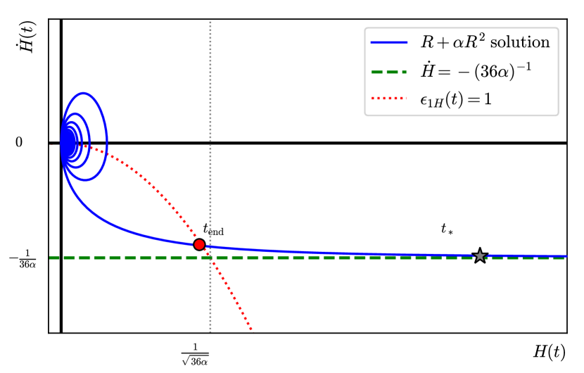
Figure 2: Diagram of a typical solution of $R+\alpha R^{2}$ inflation in the $(H,\dot{H})$ plane. The red dot indicates the end of the inflationary phase, while the gray star illustrates a point associated to a pivot scale $k_{\ast}$. When $\epsilon_{1H}\to 0$, $\dot{H}$ reduces to $-1/36\alpha$, as shown in the green dashed line. The dotted gray line indicates the approximate scale $H\approx 1/\sqrt{36\alpha}$.

Similarly, for $\epsilon_{2H}(t)$ and $\epsilon_{3H}(t)$, we find

$$\epsilon_{2H}(t) =-2\epsilon_{1H}(t)+\frac{1}{3}\epsilon_{1H}(t)^{2}-\frac{5}{9}\epsilon_{1H}(t)^{3}+\order{\epsilon^{4}}\,,$$

$$\epsilon_{3H}(t) =-2\epsilon_{1H}(t)+\frac{2}{3}\epsilon_{1H}(t)^{2}-\frac{5}{3}\epsilon_{1H}(t)^{3}+\order{\epsilon^{4}}\,,$$

$$\epsilon_{4H}(t) =-2\epsilon_{1H}(t)+\epsilon_{1H}(t)^{2}+\order{\epsilon^{3}}\,.$$ (84)

Inflation ends at a time $t_{\mathrm{end}}$ defined by $\ddot{a}(t_{\mathrm{end}})=0$ or, in terms of Hubble flow parameters (10), when $\epsilon_{1H}(t_{\textrm{end}})=1$. The expansion from a reference time $t_{\ast}$ during inflation until the end of inflation or, equivalently, the e-folding number $N_{\ast}$ in

$$a(t_{\mathrm{end}})=\mathrm{e}^{N_{\ast}}\,a(t_{\ast})\,,$$ (85)

can be computed by noticing that $N_{\ast}$ can be written as

$$N_{\ast}\equiv\int_{t_{\ast}}^{t_{\textrm{end}}}H(t)\differential{t}=-\int_{\epsilon_{1H\ast}}^{1}\frac{\differential{\epsilon_{1H}}}{\epsilon_{1H}\;\,\epsilon_{2H}\big{(}\epsilon_{1H}\big{)}},$$ (86)

where the second Hubble-flow parameter is expressed as a function of the first, $\epsilon_{2H}=\epsilon_{2H}(\epsilon_{1H})$, using (VII). Integrating order by order we find

$$N_{\ast}(\epsilon_{1H\ast}) =\frac{1}{2\epsilon_{1Hs}}+\frac{1}{8}\epsilon_{1H\ast}+\frac{19}{864}\epsilon_{1H\ast}^{2}-\frac{71}{7776}\epsilon_{1H\ast}^{3}$$

$$\quad-\frac{\ln(\epsilon_{1H\ast})}{12}+D_{0}+\order{\epsilon_{1H\ast}^{4}},$$ (87)

with

$$D_{0} \textstyle\;=-\frac{1}{2}+\frac{\ln(2)}{24}+\frac{\ln(3)}{12}-\frac{\ln(20)}{24}$$

$$\textstyle\qquad-\frac{19\tan^{-1}\left(\frac{1}{\sqrt{39}}\right)}{12\sqrt{39}}-\frac{19\cot^{-1}\left(\frac{3\sqrt{39}}{7}\right)}{12\sqrt{39}}\simeq-0.635\,.$$

It is clear that, for small values of $\epsilon_{1H\ast}$, the number of e-foldings is determined by the first term but, in our analysis of the N3LO power spectrum (with $t_{\ast}$ taken to be the time when the pivot mode $k_{\ast}$ crosses the horizon), we will need also the higher order terms. The relation (VII) can be perturbatively inverted, to find the following expression

$$\epsilon_{1H\ast}(N_{\ast})=\frac{1}{2N_{\ast}}+\frac{\frac{D_{0}}{2}-\frac{1}{24}\ln(\frac{1}{2N_{\ast}})}{N_{\ast}^{2}}\;+$$

$$\;\;+\frac{D_{1}-D_{2}\ln(\frac{1}{2N_{\ast}})+\frac{1}{288}\ln(\frac{1}{2N_{\ast}})^{2}}{N_{\ast}^{3}}+\mathcal{O}(N_{\ast}^{-4}),$$ (88)

where $D_{1}=(3-4D_{0}+48D_{0}^{2})/96\simeq 0.259$, and $D_{2}=(-1+24D_{0})/(288)\simeq-0.056$. Again, for large values of $N_{\ast}$, the main contribution comes from the first term. In the range $N_{\ast}\in[50,60]$, we have the associated range $\epsilon_{1H\ast}\in[0.00995,0.00830]$. By combining the expansions (VII) with the expression for $\epsilon_{1H\ast}$ given in (VII), we can express all the features of the power spectra for Starobinsky inflation in terms of $N_{\ast}$, up to order $\order{N_{\ast}^{-3}}$.

Table 6: Curvature and tensor perturbations for $R+\alpha R^{2}$ inflation, up to N3LO.

Quantity	Coefficients
$\begin{aligned} \mathcal{A}_{\textrm{s}}&=\frac{G\hbar\,N_{\ast}^{2}}{18\pi\alpha}\Bigg{[}1+\frac{p_{1}^{(\textrm{s})}}{N_{\ast}}-\frac{\ln(2N_{\ast})}{6N_{\ast}}\\ &\quad+\frac{p_{2}^{(\textrm{s})}}{N_{\ast}^{2}}-\,p_{2L}^{(\textrm{s})}\frac{\ln(2N_{\ast})}{N_{\ast}^{2}}+\frac{\ln(2N_{\ast})^{2}}{144N_{\ast}^{2}}\\ &\quad-p_{3L}^{(\textrm{s})}\frac{\ln(2N_{\ast})}{N_{\ast}^{3}}+p_{3L^{2}}^{(\textrm{s})}\frac{\ln(2N_{\ast})^{2}}{N_{\ast}^{3}}+\frac{\ln(2N_{\ast})^{3}}{864N_{\ast}^{3}}\\ &\quad+\frac{p_{3}^{(\textrm{s})}}{N_{\ast}^{3}}+\order{N_{\ast}^{-4}}\Bigg{]}\end{aligned}$	$\begin{aligned} p_{1}^{(\textrm{s})}&=1/2-2C-2D_{0}\simeq 3.2298819\\ p_{2}^{(\textrm{s})}&=-(283/48)+C^{2}-D_{0}/2+3D_{0}^{2}\\ &\quad+C(-(4/3)+2D_{0})-4D_{1}+(7\pi^{2})/12\\ &\simeq 2.7841172\\ p_{2L}^{(\textrm{s})}&=(1-4C-12D_{0}+96D_{2})/24\simeq 0.25526794\\ p_{3L}^{(\textrm{s})}&=D_{0}^{2}-D_{1}+1/12D_{0}(-1+4C-144D_{2})\\ &\quad+D_{2}-4CD_{2}\simeq-0.29960351\\ p_{3L^{2}}^{(\textrm{s})}&=-(D_{0}/24)+D_{2}\simeq-0.029943214\\ p_{3}^{(\textrm{s})}&=-(553/432)+(5C^{2})/12+D_{0}^{2}/2-4D_{0}^{3}\\ &\quad-D_{1}+12D_{0}D_{1}+C[-(127/72)-2D_{0}^{2}\\ &\quad+4D_{1}]+(25\pi^{2})/48-6\zeta(3)\\ &\simeq-3.0222532.\end{aligned}$
$\vspace{0.2em}\begin{aligned} ~{}\\[-12.91663pt] n_{\textrm{s}}&=1-\frac{2}{N_{\ast}}+\frac{\theta_{2}^{(\textrm{s})}}{N_{\ast}^{2}}-\frac{\ln(2N_{\ast})}{6N_{\ast}^{2}}\\ &\quad-\theta_{3L}^{(\textrm{s})}\frac{\ln(2N_{\ast})}{N_{\ast}^{3}}-\frac{\ln(2N_{\ast})^{2}}{72N_{\ast}^{3}}\\ &\quad+\frac{\theta_{3}^{(\textrm{s})}}{N_{\ast}^{3}}+\order{N_{\ast}^{-4}}\end{aligned}$	$\begin{aligned} \theta_{2}^{(\textrm{s})}&=-(1/3)-2C-2D_{0}\simeq 2.3965486\\ \theta_{3L}^{(\textrm{s})}&=1/18+C/3+4D_{2}\simeq-0.41331365\\ \theta_{3}^{(\textrm{s})}&=-(241/18)-2C^{2}-(2D_{0})/3-C(3+8D_{0})/2\\ &\quad-4D_{1}+(7\pi^{2})/6\simeq-4.3133704.\end{aligned}$
$\vspace{0.2em}\begin{aligned} ~{}\\[-12.91663pt] \alpha_{\textrm{s}}=-\frac{2}{N_{\ast}^{2}}-\frac{\ln(2N_{\ast})}{3N_{\ast}^{3}}+\frac{\alpha_{3}^{(\textrm{s})}}{N_{\ast}^{3}}+\order{N_{\ast}^{-4}}\end{aligned}$	$\alpha_{3}^{(\textrm{s})}=-(3/2)-4C-4D_{0}\simeq 3.9597638$
$\vspace{0.2em}\begin{aligned} ~{}\\[-12.91663pt] &\beta_{\textrm{s}}=-\frac{4}{N_{\ast}^{3}}+\order{N_{\ast}^{-4}}\end{aligned}$
$\vspace{0.2em}\begin{aligned} ~{}\\[-12.91663pt] \mathcal{A}_{\textrm{t}}&=\frac{2G\hbar}{3\pi\alpha}\Bigg{[}1-\frac{3}{2N_{\ast}}\\ &\quad+\frac{p_{2}^{(\textrm{t})}}{N_{\ast}^{2}}-\frac{\ln(2N_{\ast})}{8N_{\ast}^{2}}\\ &\quad-p_{3L}^{(\textrm{t})}\frac{\ln(2N_{\ast})}{N_{\ast}^{3}}-\frac{\ln(2N_{\ast})^{2}}{96N_{\ast}^{3}}+\frac{p_{3}^{(\textrm{t})}}{N_{\ast}^{3}}+\order{N_{\ast}^{-4}}\Bigg{]}\end{aligned}$	$\begin{aligned} p_{2}^{(\textrm{t})}&=-(1+24C+24D_{0})/16\simeq 1.9849114\\ p_{3L}^{(\textrm{t})}&=1/96+C/4+3D_{2}\simeq-0.34123524\\ p_{3}^{(\textrm{t})}&=-[85+72C^{2}+6D_{0}+36C(1+4D_{0})\\ &\qquad+144D_{1}-6\pi^{2}]/48\simeq-2.8782506.\end{aligned}$
$\begin{aligned} ~{}\\[-8.61108pt] n_{\textrm{t}}&=-\frac{3}{2N_{\ast}^{2}}-\frac{\ln(2N_{\ast})}{4N_{\ast}^{3}}+\frac{\theta_{3}^{(\textrm{t})}}{N_{\ast}^{3}}+\order{N_{\ast}^{-4}}\end{aligned}$	$\begin{aligned} \theta_{3}^{(\textrm{t})}=-3(C+D_{0}+1)\simeq 1.0948228\end{aligned}$
$\begin{aligned} ~{}\\[-12.91663pt] \alpha_{\textrm{t}}=-\frac{3}{N_{\ast}^{3}}+\order{N_{\ast}^{-4}}\end{aligned}$
$\begin{aligned} ~{}\\[-12.91663pt] &\beta_{\textrm{s}}=0+\order{N_{\ast}^{-4}}\end{aligned}$
$\vspace{0.3em}\begin{aligned} ~{}\\[-12.91663pt] r\equiv\dfrac{\mathcal{A}_{\textrm{t}}}{\mathcal{A}_{\textrm{s}}}=\dfrac{12}{N_{\ast}^{2}}+\dfrac{2\ln(2N_{\ast})}{N_{\ast}^{3}}-r_{3}\dfrac{24}{N_{\ast}^{3}}+\order{N_{\ast}^{-4}}\end{aligned}$	$r_{3}=1-C-D_{0}\simeq 2.3649409$
$\begin{aligned} ~{}\\[-10.00002pt] &\delta\equiv r+8n_{\textrm{t}}=-\frac{48}{N_{\ast}^{3}}+\order{N_{\ast}^{-4}}\end{aligned}$

Perturbations

We derive the quadratic action for SVT perturbations in Starobinsky inflation, working purely in the geometric framework. The starting point is the tensor $F^{\mu\nu}[g_{\mu\nu}]$ obtained from the variation of the action (76),

$$F^{\mu\nu}[g_{\mu\nu}]\equiv\functionalderivative{S}{g_{\mu\nu}}\,=\,-\frac{1}{16\pi G}\sqrt{-g}\,\big{(}G^{\mu\nu}+\alpha\mathcal{H^{\mu\nu}}\big{)}\,,$$ (89)

where we used (80)–(81) and $\delta g_{\mu\nu}=-g_{\mu\alpha}g_{\nu\beta}\delta g^{\alpha\beta}$. Expanding around the FLRW metric (3), we write

$$F^{\mu\nu}[\bar{g}_{\mu\nu}+\delta g_{\mu\nu}]=\bar{F}_{0}^{\mu\nu}(t)\,+\,\bar{F}_{1}^{\mu\nu\rho\sigma}(t)\,\delta g_{\rho\sigma}+\mathcal{O}(\delta g^{2})\,.$$

As we assume that the backgound metric satisfies the Friedman equation (82), the term $\bar{F}_{0}^{\mu\nu}=0$ vanishes. Therefore, the action (76), at quadratic order in the perturbation, can be written as

$$S[\bar{g}_{\mu\nu}+\delta g_{\mu\nu}]=\bar{S}(t)+\int\!\differential[4]{x}\tfrac{1}{2}\,\delta g_{\mu\nu}\bar{F}_{1}^{\mu\nu\rho\sigma}(t)\,\delta g_{\rho\sigma}+\mathcal{O}(\delta g^{3})\,.$$ (90)

We can then use the homogeneity and isotropy of the background to organize perturbations into scalar, vector and tensor (SVT) representations of the $3d$ Euclidean group, $\delta g_{\mu\nu}=\delta g^{(\mathrm{s})}_{\mu\nu}+\delta g^{(\mathrm{v})}_{\mu\nu}+\delta g^{(\mathrm{t})}_{\mu\nu}$ which in the quadratic action decouple, as most easily shown by working in Fourier transform.

Let us consider scalar perturbations first. In Fourier transform (5), using the language of ADM variables $g_{\mu\nu}\differential x^{\mu}\differential{x}^{\nu}=-N^{2}\differential{t}^{2}+h_{ij}(N^{i}\differential{t}+\differential{y}^{i})(N^{j}\differential{t}+\differential{y}^{j})$ (with $i,j=1,2,3$), the perturbation $\delta g^{(\mathrm{s})}_{\mu\nu}$ can be written in terms of the lapse $N=1+\delta N$ and of the shift $N^{i}=0+\delta N^{i}$, with scalar perturbations $\delta N$ and $S$,

$$\delta N(\mathbf{k},t),$$ (91)

$$\delta N^{i}(\mathbf{k},t)=\mathrm{i}\,k^{i}S(\mathbf{k},t)\,$$ (92)

together with the $3d$ metric $h_{ij}=a(t)^{2}\delta_{ij}+\delta h_{ij}^{(\mathrm{s})}$, with scalar perturbations $\mathcal{R}$ and $\mathcal{C}$

$$\delta h_{ij}^{(\mathrm{s})}(\mathbf{k},t)=-2\,\mathcal{R}(\mathbf{k},t)a(t)^{2}\delta_{ij}-k_{i}k_{j}\,\mathcal{C}(\mathbf{k},t)\,.$$ (93)

We work in the comoving gauge $\mathcal{H}^{0}{}_{i}=0$, which generalizes the comoving gauge $T^{0}{}_{i}=0$ for the energy-momentum in general relativity with matter. Solving perturbatively the Hamitonian constraint $F^{0}{}_{0}\approx 0$ and the diffeomorphism constraint $F^{0}{}_{i}\approx 0$, we can express the scalar perturbations $\delta N(\mathbf{k},t)$, $\delta N^{i}$ and $\mathcal{C}$ in terms of the curvature perturbation $\mathcal{R}$. At first order in the perturbation, constant-$t$ spatial sections have scalar curvature given by the $3d$ Ricci scalar ${}^{(3)\!}R=4a(t)^{-2}\,\delta^{ij}\partial_{i}\partial_{j}\mathcal{R}$. Substituting these expressions into (90), and introducing the useful definitions

$$\chi(t) \equiv 1+2\alpha\bar{R}(t)=1+24\alpha H(t)^{2}(1-\tfrac{1}{2}\epsilon_{1H}(t))\,,$$ (94)

$$\epsilon_{\chi}(t) =-\frac{\dot{\chi}(t)}{H(t)\,\chi(t)}\,,$$ (95)

we find that the quadratic action for the single scalar mode, the curvature perturbation $\mathcal{R}(\mathbf{k},t$), takes the form (4) with kinetic amplitude and speed of sound:

$$Z_{\textrm{s}}(t)\, =\frac{3\chi(t)}{16\pi G}\quantity(\frac{\epsilon_{\chi}(t)}{1+\frac{1}{2}\epsilon_{\chi}(t)})^{2}\,,$$ (96)

$$c_{\textrm{s}}(t)\, =\,1\,.$$ (97)

For vector perturbations, working in the same comoving gauge, introducing the transverse vector fields $\delta N^{a}_{T}$ for the shift and $B_{a}(\mathbf{x},t)$ for the ADM metric $\delta h_{ab}^{(\mathrm{v})}(\mathbf{k},t)=\mathrm{i}\,a(t)(k_{a}B_{b}(\mathbf{x},t)+k_{b}B_{a}(\mathbf{k},t))$, and solving the transverse part of the diffeomorphism constraint, one finds as usual that there is no propagating vectorial perturbation. Finally, for transverse-traceless tensor perturbations

$$\delta h_{ab}^{(\mathrm{t})}(\mathbf{k},t)=e_{ab}^{(+)}(\mathbf{k})\gamma_{(+)}(\mathbf{k},t)+e_{ab}^{(-)}(\mathbf{k})\gamma_{(-)}(\mathbf{k},t)\,,$$ (98)

one finds again that the action takes the form (4) with kinetic amplitude and speed of sound:

$$Z_{\textrm{t}}(t)\, =\frac{\chi(t)}{64\pi G}\,,$$ (99)

$$c_{\textrm{t}}(t)\, =\,1\,.$$ (100)

As a check of this expression, note that in the geometric framework for Starobinsky inflation discussed here, the kinetic amplitude of tensor modes (99) reduces to the familiar one in general relativity (75) in the limit $\alpha\to 0$. Note also that these expressions for the kinetic amplitude and speed of sound are exact as we did not use up to this point any Hubble-flow expansion.

Power spectrum

Let us now use the Hubble-flow expansion to express the kinetic amplitude in terms of a series in the single parameter $\epsilon_{1H\ast}$, the first Hubble flow parameter evaluated at the pivot time $t_{\ast}$. For scalar perturbations we find

$$Z_{\textrm{s}\ast} =\frac{\epsilon_{1H\ast}}{2\pi G}\left[1-\frac{19}{6}\epsilon_{1H\ast}+\frac{74}{9}\epsilon_{1H\ast}^{2}\right]+\order{\epsilon_{1H\ast}^{4}}\,,$$ (101)

with Hubble-flow parameters for $Z_{\textrm{s}}$ given by

$$\epsilon_{1Z\ast}^{(\textrm{s})} =-2\epsilon_{1H\ast}+\frac{20}{3}\epsilon_{1H\ast}^{2}-\frac{130}{9}\epsilon_{1H\ast}^{3}+\order{\epsilon_{1H\ast}^{4}}\,,$$

$$\epsilon_{2Z\ast}^{(\textrm{s})} =-2\epsilon_{1H\ast}+7\epsilon_{1H\ast}^{2}-\frac{25}{3}\epsilon_{1H\ast}^{3}+\order{\epsilon_{1H\ast}^{4}}\,,$$

$$\epsilon_{3Z\ast}^{(\textrm{s})} =-2\epsilon_{1H\ast}+\frac{22}{3}\epsilon_{1H\ast}^{2}+\frac{37}{3}\epsilon_{1H\ast}^{3}+\order{\epsilon_{1H\ast}^{4}}\,.$$ (102)

For tensor perturbations we find

$$Z_{\textrm{t}\ast} =\frac{1}{96\pi G\epsilon_{1H\ast}}\left[1+\frac{5}{6}\epsilon_{1H\ast}+\frac{2}{9}\epsilon_{1H\ast}^{2}\right.$$

$$\qquad\left.-\frac{8}{27}\epsilon_{1H\ast}^{3}+\frac{2}{3}\epsilon_{1H\ast}^{4}\right]+\order{\epsilon_{1H\ast}^{4}}\,,$$ (103)

with Hubble-flow parameters for $Z_{\textrm{t}}$ given by

$$\epsilon_{1Z\ast}^{(\textrm{t})} =2\epsilon_{1H\ast}-2\epsilon_{1H\ast}^{2}+\frac{4}{3}\epsilon_{1H\ast}^{3}+\order{\epsilon_{1H\ast}^{4}}\,,$$

$$\epsilon_{2Z\ast}^{(\textrm{t})} =-2\epsilon_{1H\ast}+\frac{7}{3}\epsilon_{1H\ast}^{2}-\frac{14}{9}\epsilon_{1H\ast}^{3}+\order{\epsilon_{1H\ast}^{4}}\,,$$

$$\epsilon_{3Z\ast}^{(\textrm{t})} =-2\epsilon_{1H\ast}+\frac{8}{3}\epsilon_{1H\ast}^{2}-\frac{4}{3}\epsilon_{1H\ast}^{3}+\order{\epsilon_{1H\ast}^{4}}\,.$$ (104)

We can substitute the expressions found above into the the general formulas reported in Tab. 2 and 3, together with the expression (VII) for the first Hubble flow parameter in terms of the number of e-foldings $N_{\ast}$, to find the N3LO formulas for the power spectrum of $R+\alpha R^{2}$ inflation, which are reported in Tab. 6.

Given the phenomenological success of $R+\alpha R^{2}$ inflation in accounting for current cosmological observations of primordial perturbations, it is useful to comment on the accuracy of its predictions. First of all, we note that observational constraints of the scalar tilt $n_{\mathrm{s}}$, result in a preferred value for the number of inflationary e-foldings

$$N_{\ast}=56.2\pm 7.8\,.$$ (105)

Moreover, since the amplitude of curvature perturbation is constrained to be $\ln(10^{10}\mathcal{A}_{\textrm{s}})=3.044\pm 0.014$, the preferred value of the coupling constant $\alpha$ is

$$\alpha=(2.777\pm 0.779)\times 10^{10}\,G\hbar\simeq(2.7\times 10^{-30}\,\textrm{m})^{2}\,,$$ (106)

which results in a prediction for the tensor-to-scalar ratio (for the range $N_{\ast}=55\pm 5$)

$$r=(3.767\pm 0.652)\times 10^{-3}\quad\textrm{at N3LO}\,.$$ (107)

Note that the N3LO corrections are non-negligible and result in a decrease by $7\%$ of the predicted tensor-to-scalar ratio at NLO, (See Fig. 1). It is interesting to remark also that if in the near future an amplitude $\mathcal{A}_{\mathrm{t}}\sim G\hbar/\alpha$ of tensor modes is observed, it will provide evidence for the quantization of gravity [54]. The geometric framework discussed here highlights how the observed amplitude $\mathcal{A}_{\mathrm{s}}\sim(G\hbar/\alpha)N_{\ast}^{2}$ of scalar perturbations via CMB temperature anisotropy already provides a probe of (perturbative) quantum gravity, as implied the Planck area $\ell_{P}^{2}=G\hbar$ in this expression.

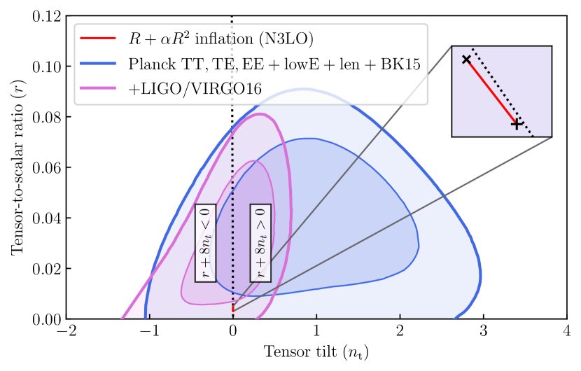
Figure 3: Marginalized joint 68% and 95% C.L. regions for $n_{t}$ and $r$ at $0.01$ Mpc^-1 as reported by the Planck Collaboration [11]. The orange region of LIGO/VIRGO is associated to the constraints on the stochastic gravitational-wave background, i.e., $\Omega_{\textrm{GW}}$ [55]. The dotted black line illustrates the exact consistency relation $r=-8n_{t}$. The $\crossproduct$ ($+$) indicate $N_{\ast}=50\,(60)$ for Starobinsky inflation.

The N3LO calculation allows us to identify also the order of magnitude of violation of the single-field consistency condition, generally stated as $r=-8n_{\textrm{t}}$ at LO [56]. The formalism developed in this work provides a precise prediction of the amount of deviation from this condition for $R+\alpha R^{2}$ inflation,

$$\delta\equiv r+8n_{\textrm{t}}=-\frac{48}{N_{\ast}^{3}}+\order{N_{\ast}^{-4}}.$$ (108)

This result can be compared to the constraints imposed by Planck and LIGO/VIRGO on $r$ and $n_{\mathrm{t}}$, as shown in Fig. 3: the predicted value is within the confidence level regions, with $n_{\mathrm{t}}$ and $\delta$ predicted to be (for the range $N_{\ast}=55\pm 5$)

$$n_{\mathrm{t}} =(-5.088\pm 0.917)\times 10^{-4}\quad\textrm{at N3LO}\,,$$ (109)

$$\delta =(-3.031\pm 0.809)\times 10^{-4}\quad\textrm{at N3LO}\,.$$ (110)

Moreover, we find that $R+\alpha R^{2}$ inflation predicts a value running and running of the running for the scalar power spectrum

$$\alpha_{\textrm{s}} =(-6.626\pm 1.180)\times 10^{-4}\quad\textrm{at N3LO}\,,$$ (111)

$$\beta_{\textrm{s}} =(-2.526\pm 0.674)\times 10^{-5}\quad\textrm{at N3LO}\,.$$ (112)

These values are within the current constraints reported by Planck, as illustrated in Fig. 4. Note also that the predicted value of the running $\alpha_{\textrm{s}}$ is negative and consistent with the $68\%$ C.L. interval $\alpha_{\textrm{s}}=(-6.75\pm 2.05)\times 10^{-4}$ recently obtained in [57] using the posterior probability distribution marginalized over nearly $300$ models of single-field inflation.

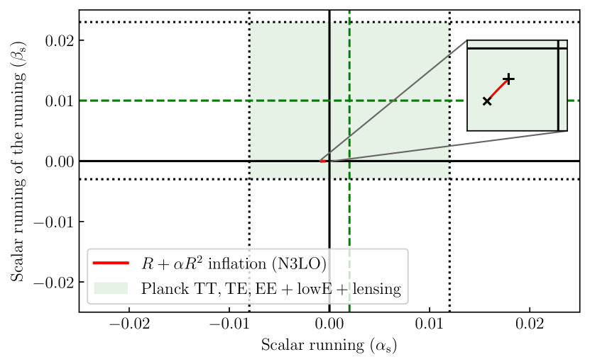
Figure 4: Schematic visualization of the constraints on the running and the running of the running of the scalar tilt. The solid black lines indicate $\alpha_{\textrm{s}}=\beta_{\textrm{s}}=0$, and the dashed green lines the values $\alpha_{\textrm{s}}=0.002\pm 0.010$ and $\beta_{\textrm{s}}=0.010\pm 0.013$, as reported by the Planck Collaboration, both at 68% C.L. [11]. The $\crossproduct$ ($+$) indicate $N_{\ast}=50\,(60)$ for Starobinsky inflation.

VIII Discussion

Table 7: Summary of results.

Result	Where to find it
Generic $Z_{\psi}$, $c_{\psi}$	$\vspace{0.2em}\begin{aligned} ~{}\\[-12.91663pt] &\textrm{Amplitude}\;\mathcal{A}_{\ast}^{(\psi)}:\textrm{Tab. \ref{Tab:GenericTheory-Amplitude} }\\ &\textrm{Features}\;\theta_{\ast}^{(\psi)},\alpha_{\ast}^{(\psi)},\beta_{\ast}^{(\psi)}:\,\textrm{Tab. \ref{Tab:GenericTheory-Features}}\end{aligned}$
Scalar field	$\vspace{0.2em}\begin{aligned} ~{}\\[-12.91663pt] &\textrm{Scalar}\;\mathcal{A}_{\textrm{s}},n_{\textrm{s}},\alpha_{\textrm{s}},\beta_{\textrm{s}}:\;\textrm{Tab. \ref{Tab:SingleField-ScalarFeatures}}\\ &\textrm{Tensor}\;\mathcal{A}_{\textrm{t}},n_{\textrm{t}},\alpha_{\textrm{t}},\beta_{\textrm{t}}:\;\textrm{Tab. \ref{Tab:SingleField-TensorFeatures}}\end{aligned}$
$R+\alpha R^{2}$	$\vspace{0.2em}\begin{aligned} ~{}\\[-12.91663pt] &\mathcal{A}_{\textrm{s,t}},n_{\textrm{s,t}},\alpha_{\textrm{s,t}},\beta_{\textrm{s,t}}:\;\textrm{Tab. \ref{Tab:Starobinsky-Results}}\end{aligned}$

In this paper we derived N3LO expressions for the primordial power spectrum and its features in a broad class of effective theories of inflation with action for perturbations of the form (4). We adopted the Green’s function method [17, 18] to compute the late-time behavior of the mode functions of the quasi-Bunch-Davies initial state at N3LO, assuming a sufficiently long quasi-de Sitter inflationary phase $(N\gg N_{\ast})$. Our main results are summarized in Tab. 7.

Current measurements of primordial observables already probe the amplitude and tilt of scalar modes, and provide contraints on the amplitude and tilt of tensor modes [11]. The next generation of CMB experiments, such as CMB-S4 [15], LiteBIRD[16], CORE [14], PICO [58] or surveys such as the Simons Observatory [59] or EUCLID [60], is expected to measure N2LO corrections and put stronger constraints on N3LO terms, under the assumption of single-field inflation. In this work we introduced a framework that covers up to N3LO all effective models parametrized by the two functions $Z(t)$ and $c(t)$, treated as independent here. As illustrated in Tab. 1, many effective theories fit within the framework developed in this paper. In the case of $R+\alpha R^{2}$ Starobinsky inflation, we computed the N3LO corrections, expressing them explicitly in terms of one single free parameter—the number of inflationary e-foldings $N_{\ast}$ from the exit of the pivot mode $k_{\ast}$ until the end of inflation. The explicit expressions are reported in Tab. 6. We expect these results to be useful to further test this model with even more precise CMB observations in the future, as illustrated in Fig. 3 and 4.

The fact that the primordial power spectrum probes physics at a scale that is only $\sim 5$ orders of magnitude away from the Planck length $\ell_{P}$ is remarkable. This is a regime that lies at the interface of effective field theory and quantum gravity. While, on the one hand, it is important to identify top-down derivations of the cosmological regime of quantum gravity theories such as [25, 26, 61, 62, 63], on the other hand, working at this interface where one parametrizes quantum gravity effects into an effective field theory can allow us to put observational constraints and identify features of quantum geometry in the CMB sky [64]. In particular, it would be interesting to develop a similar N3LO framework for functions $Z_{\mathrm{t}}(t,k)$ and $c_{\mathrm{t}}(t,k)$ with a Fourier mode dependence, such as the ones that appear in models with a parity-violating coupling to the Chern-Simons density [29]. In fact, extracting precise predictions for effective theories such as [65] and [66] could allow us to distinguish quantum gravity theories with observations of primordial parity violation.

Appendix A Generalized conformal time with speed of sound

In conformal time $\eta$, the FLRW metric takes the form

$$\bar{g}_{\mu\nu}\differential{x}^{\mu}\differential{x}^{\nu}=a(t)^{2}\big{(}-\differential{\eta}^{2}+\delta_{ij}\differential{x}^{i}\differential{x}^{j}\big{)},$$ (113)

which corresponds to the following relation to the cosmic time $t$,

$$\derivative{\eta}{t}=\frac{1}{a(t)}.$$ (114)

In de Sitter space we have the exact relation $\eta_{\textrm{dS}}=-1/(aH_{0})$. Here we consider the case of quasi-de Sitter with, in addition, a speed of sound $c_{\psi}\neq 1$. We recall the definition $x=-k_{\ast}\eta$ together with (32). The goal is to write

$$\derivative{\eta}{t}=\frac{c_{\psi}(t)}{a(t)}=-\derivative{t}\quantity(\frac{c_{\psi}(t)}{a(t)H(t)})+\;\textrm{corrections},$$ (115)

in an order-by-order expansion. At zero order, we can start with the ansatz

$$\eta_{\textrm{ansatz}}^{(0)}=-\frac{c_{\psi}(t)}{a(t)H(t)}\quad\to\quad\frac{c_{\psi}(t)}{a(t)}-\derivative{t}\eta_{\textrm{ansatz}}^{(0)}=0+\order{\epsilon}\quad\to\quad\eta^{(0)}=-\frac{c_{\psi}(t)}{a(t)H(t)}\,.$$ (116)

For the next order, we consider the most general ansatz of order one,

$$\eta_{\textrm{ansatz}}^{(1)}=-\frac{c_{\psi}(t)}{a(t)H(t)}\quantity(1+b_{1}\epsilon_{1H}(t)+b_{2}\epsilon_{1c}(t))\;\to\;\frac{c_{\psi}(t)}{a(t)}-\derivative{t}\eta_{\textrm{ansatz}}^{(1)}=-\frac{c_{\psi}(t)((b_{1}-1)\epsilon_{1H}(t)+(b_{2}+1)\epsilon_{1c}(t))}{a(t)}+\order{\epsilon^{2}},$$ (117)

which vanishes for $b_{1}=1$ and $b_{2}=-1$. Hence,

$$\eta^{(1)}=-\frac{c_{\psi}(t)}{a(t)H(t)}\quantity(1+\epsilon_{1H}(t)-b_{2}\epsilon_{1c}(t)).$$ (118)

Similarly, at the next order we have

$$\eta_{\textrm{ansatz}}^{(2)} =-\frac{c(t)}{a(t)H(t)}\Big{(}1+\epsilon_{1H}(t)-\epsilon_{1c}(t)+c_{11}\epsilon_{1H}(t)^{2}+c_{22}\epsilon_{2H}(t)^{2}+c_{12}\epsilon_{1H}(t)\epsilon_{2H}(t)+b_{11}\epsilon_{1c}(t)^{2}+b_{22}\epsilon_{2c}(t)^{2}$$

$$\qquad+b_{12}\epsilon_{1c}(t)\epsilon_{2c}(t)+bc_{1}\epsilon_{1c}(t)\epsilon_{1H}(t)+bc_{2}\epsilon_{2c}(t)\epsilon_{1H}(t)+bc_{3}\epsilon_{1c}(t)\epsilon_{2H}(t)+bc_{4}\epsilon_{2c}(t)\epsilon_{2H}(t)\Big{)}\,.$$ (119)

After replacing the ansatz, we find that

$$\frac{c_{\psi}(t)}{a(t)}-\derivative{t}\eta_{\textrm{ansatz}}^{(2)}=0+\order{\epsilon^{3}}$$ (120)

for $c_{11}\to 1,c_{12}\to-1,c_{22}\to 0,b_{11}\to 1,b_{22}\to 0,bc_{4}\to 0,c_{22}\to 0,bc1\to-2,b_{12}\to 1,bc_{3}\to 0,bc_{2}\to 0,c_{12}\to-1$. Then, up to second order,

$$\eta^{(2)} =-\frac{c_{\psi}(t)}{a(t)H(t)}\Big{[}1+\epsilon_{1H}(t)-\epsilon_{1c}(t)+\epsilon_{1H}(t)^{2}-\epsilon_{1H}(t)\epsilon_{2H}(t)-2\epsilon_{1c}(t)\epsilon_{1H}(t)+\epsilon_{1c}(t)\epsilon_{2c}(t)+\epsilon_{1c}(t)^{2}\Big{]}\,.$$ (121)

The same procedure can be extended order by order. In particular, for the next order we need to assume an ansatz with all the possible combinations of third order quantities. Repeating the same process, we find that the conformal time up to third order is given by,

$$\eta^{(3)} =-\frac{c_{\psi}(t)}{a(t)H(t)}\Big{[}1+\epsilon_{1H}(t)-\epsilon_{1c}(t)+\epsilon_{1H}(t)^{2}-\epsilon_{1H}(t)\epsilon_{2H}(t)-2\epsilon_{1c}(t)\epsilon_{1H}(t)+\epsilon_{1c}(t)\epsilon_{2c}(t)+\epsilon_{1c}(t)^{2}$$

$$\quad+\epsilon_{1H}(t)^{3}+\epsilon_{1H}(t)\epsilon_{2H}(t)\epsilon_{3H}(t)-3\epsilon_{1H}(t)^{2}\epsilon_{2H}(t)+\epsilon_{1H}(t)\epsilon_{2H}(t)^{2}-\epsilon_{1c}(t)\epsilon_{2c}(t)^{2}+3\epsilon_{1c}(t)\epsilon_{1H}(t)\epsilon_{2H}(t)$$

$$\quad-3\epsilon_{1c}(t)^{2}\epsilon_{2c}(t)+3\epsilon_{1c}(t)\epsilon_{1H}(t)\epsilon_{2c}(t)-\epsilon_{1c}(t)\epsilon_{2c}(t)\epsilon_{3c}(t)-\epsilon_{1c}(t)^{3}+3\epsilon_{1c}(t)^{2}\epsilon_{1H}(t)-3\epsilon_{1c}(t)\epsilon_{1H}(t)^{2}\Big{]}\,.$$ (122)

Appendix B Coefficients for the power spectrum in a theory with generic $Z_{\psi}$ and $c_{\psi}$

We report the N3LO coefficients $p_{0\ast}$, $p_{1\ast}$, $p_{2\ast}$, $p_{3\ast}$:

$$p_{0\ast} =(2+3C)\epsilon_{1c\ast}-2(1+C)\epsilon_{1H\ast}+C\epsilon_{1Z\ast}$$

$$\quad+\frac{1}{24}\left(3(-64+24C+36C^{2}+9\pi^{2})\epsilon_{1c\ast}^{2}+12(-6+4C+4C^{2}+\pi^{2})\epsilon_{1H\ast}^{2}\right.$$

$$\quad\left.-3\epsilon_{1c\ast}\left(4(-20+10C+12C^{2}+3\pi^{2})\epsilon_{1H\ast}-2(-24+4C+12C^{2}+3\pi^{2})\epsilon_{1Z\ast}+(16+16C+12C^{2}-\pi^{2})\epsilon_{2c\ast}\right)\right.$$

$$\quad\left.-2\epsilon_{1H\ast}\left(6(-8+2C+4C^{2}+\pi^{2})\epsilon_{1Z\ast}-24-24C-12C^{2}+\pi^{2})\epsilon_{2H\ast}\right)\right.$$

$$\quad\left.+\epsilon_{1Z\ast}\left(3(-8+4C^{2}+\pi^{2})\epsilon_{1Z\ast}-12C^{2}+\pi^{2})\epsilon_{2Z\ast}\right)\right)\epsilon^{2}$$

$$\qquad+\frac{1}{12}\epsilon_{1H\ast}\epsilon_{2H\ast}\epsilon_{3H\ast}(-12C^{2}-4C^{3}+\pi^{2}+C(-24+\pi^{2})-8(1+\zeta(3)))$$

$$\qquad+\frac{1}{12}\epsilon_{1H\ast}\epsilon_{2H\ast}^{2}(-12C^{2}-4C^{3}+\pi^{2}+C(-24+\pi^{2})-8(1+\zeta(3)))$$

$$\qquad+\frac{1}{8}(96-36C^{2}-36C^{3}-13\pi^{2}-15C(-8+\pi^{2}))\epsilon_{1c\ast}^{2}\epsilon_{2c\ast}+(-8+3C^{2}+3C^{3}+\frac{13\pi^{2}}{12}+\frac{5}{4}C(-8+\pi^{2}))\epsilon_{1c\ast}\epsilon_{1H\ast}\epsilon_{2c\ast}$$

$$\qquad+\frac{1}{24}(96-36C^{2}-36C^{3}-13\pi^{2}-15C(-8+\pi^{2}))\epsilon_{1c\ast}\epsilon_{1Z\ast}\epsilon_{2c\ast}+(8-\frac{3C^{2}}{2}-2C^{3}-\frac{13\pi^{2}}{12}+C(6-\frac{5\pi^{2}}{6}))\epsilon_{1H\ast}^{2}\epsilon_{2H\ast}$$

$$\qquad+(-12+\frac{9C^{2}}{2}+3C^{3}+\frac{13\pi^{2}}{8}+C(-9+\frac{5\pi^{2}}{4}))\epsilon_{1c\ast}\epsilon_{1H\ast}\epsilon_{2H\ast}+(-4+\frac{3C^{2}}{2}+C^{3}+\frac{13\pi^{2}}{24}+C(-3+\frac{5\pi^{2}}{12}))\epsilon_{1H\ast}\epsilon_{1Z\ast}\epsilon_{2H\ast}$$

$$\qquad-\frac{1}{8}C(-48+12C^{2}+5\pi^{2})\epsilon_{1c\ast}\epsilon_{1Z\ast}\epsilon_{2Z\ast}+C(-4+C^{2}+\frac{5\pi^{2}}{12})\epsilon_{1H\ast}\epsilon_{1Z\ast}\epsilon_{2Z\ast}-\frac{1}{24}C(-48+12C^{2}+5\pi^{2})\epsilon_{1Z\ast}^{2}\epsilon_{2Z\ast}$$

$$\qquad+\frac{1}{24}\epsilon_{1Z\ast}\epsilon_{2Z\ast}^{2}(4C^{3}-C\pi^{2}+8(-2+\zeta(3)))+\frac{1}{24}\epsilon_{1Z\ast}\epsilon_{2Z\ast}\epsilon_{3Z\ast}(4C^{3}-C\pi^{2}+8(-2+\zeta(3)))$$

$$\qquad+\epsilon_{1c\ast}\epsilon_{1H\ast}\epsilon_{1Z\ast}(24-6C^{3}-\frac{9}{2}C(-8+\pi^{2})-21\zeta(3))+\frac{1}{3}\epsilon_{1H\ast}^{3}(16-4C^{3}-3C(-8+\pi^{2})-14\zeta(3))$$

$$\qquad+\epsilon_{1H\ast}\epsilon_{1Z\ast}^{2}(4-C^{3}-\frac{3}{4}C(-8+\pi^{2})-\frac{7\zeta(3)}{2})+\epsilon_{1c\ast}\epsilon_{2c\ast}^{2}(C^{2}+\frac{C^{3}}{2}-\frac{\pi^{2}}{12}+C(2-\frac{\pi^{2}}{8})+\zeta(3))$$

$$\qquad+\epsilon_{1c\ast}\epsilon_{2c\ast}\epsilon_{3c\ast}(C^{2}+\frac{C^{3}}{2}-\frac{\pi^{2}}{12}+C(2-\frac{\pi^{2}}{8})+\zeta(3))+\epsilon_{1H\ast}^{2}\epsilon_{1Z\ast}(-8+2C^{3}+\frac{3}{2}C(-8+\pi^{2})+7\zeta(3))$$

$$\qquad+\frac{9}{8}\epsilon_{1c\ast}^{3}(4C^{3}+3C(-8+\pi^{2})+2(-8+7\zeta(3)))-\frac{9}{4}\epsilon_{1c\ast}^{2}\epsilon_{1H\ast}(4C^{3}+3C(-8+\pi^{2})+2(-8+7\zeta(3)))$$

$$\qquad+\frac{9}{8}\epsilon_{1c\ast}^{2}\epsilon_{1Z\ast}(4C^{3}+3C(-8+\pi^{2})+2(-8+7\zeta(3)))+\frac{3}{8}\epsilon_{1c\ast}\epsilon_{1Z\ast}^{2}(4C^{3}+3C(-8+\pi^{2})+2(-8+7\zeta(3)))$$

$$\qquad+\frac{1}{24}\epsilon_{1Z\ast}^{3}(4C^{3}+3C(-8+\pi^{2})+2(-8+7\zeta(3)))+\epsilon_{1c\ast}\epsilon_{1H\ast}^{2}(6C^{3}+\frac{9}{2}C(-8+\pi^{2})+3(-8+7\zeta(3)))$$ (123)

$$p_{1\ast} =3\epsilon_{1c\ast}-2\epsilon_{1H\ast}+\epsilon_{1Z\ast}$$

$$\quad+\Big{(}(3+9C)\epsilon_{1c\ast}^{2}+(-5-12C)\epsilon_{1c\ast}\epsilon_{1H\ast}+(2+4C)\epsilon_{1H\ast}^{2}+(1+6C)\epsilon_{1c\ast}\epsilon_{1Z\ast}+(-1-4C)\epsilon_{1H\ast}\epsilon_{1Z\ast}+C\epsilon_{1Z\ast}^{2}$$

$$\quad+(-2-3C)\epsilon_{1c\ast}\epsilon_{2c\ast}+2(1+C)\epsilon_{1H\ast}\epsilon_{2H\ast}-C\epsilon_{1Z\ast}\epsilon_{2Z\ast}\Big{)}$$

$$\qquad+\Big{\{}\frac{27}{8}(-8+4C^{2}+\pi^{2})\epsilon_{1c\ast}^{3}-\frac{27}{4}(-8+4C^{2}+\pi^{2})\epsilon_{1c\ast}^{2}\epsilon_{1H\ast}+\frac{9}{2}(-8+4C^{2}+\pi^{2})\epsilon_{1c\ast}\epsilon_{1H\ast}^{2}+(8-4C^{2}-\pi^{2})\epsilon_{1H\ast}^{3}$$

$$\qquad+\frac{27}{8}(-8+4C^{2}+\pi^{2})\epsilon_{1c\ast}^{2}\epsilon_{1Z\ast}-\frac{9}{2}(-8+4C^{2}+\pi^{2})\epsilon_{1c\ast}\epsilon_{1H\ast}\epsilon_{1Z\ast}+\frac{3}{2}(-8+4C^{2}+\pi^{2})\epsilon_{1H\ast}^{2}\epsilon_{1Z\ast}$$

$$\qquad+\frac{9}{8}(-8+4C^{2}+\pi^{2})\epsilon_{1c\ast}\epsilon_{1Z\ast}^{2}-\frac{3}{4}(-8+4C^{2}+\pi^{2})\epsilon_{1H\ast}\epsilon_{1Z\ast}^{2}+\frac{1}{8}(-8+4C^{2}+\pi^{2})\epsilon_{1Z\ast}^{3}$$

$$\qquad-\frac{3}{8}(24C+36C^{2}+5(-8+\pi^{2}))\epsilon_{1c\ast}^{2}\epsilon_{2c\ast}+\frac{1}{4}(24C+36C^{2}+5(-8+\pi^{2}))\epsilon_{1c\ast}\epsilon_{1H\ast}\epsilon_{2c\ast}$$

$$\qquad+\frac{1}{8}(-24C-36C^{2}-5(-8+\pi^{2}))\epsilon_{1c\ast}\epsilon_{1Z\ast}\epsilon_{2c\ast}+\frac{1}{8}(16+16C+12C^{2}-\pi^{2})\epsilon_{1c\ast}\epsilon_{2c\ast}^{2}$$

$$\qquad+\frac{1}{4}(-36+36C+36C^{2}+5\pi^{2})\epsilon_{1c\ast}\epsilon_{1H\ast}\epsilon_{2H\ast}+\frac{1}{6}(36-36C-36C^{2}-5\pi^{2})\epsilon_{1H\ast}^{2}\epsilon_{2H\ast}$$

$$\qquad+\frac{1}{12}(-36+36C+36C^{2}+5\pi^{2})\epsilon_{1H\ast}\epsilon_{1Z\ast}\epsilon_{2H\ast}+\frac{1}{12}(-24-24C-12C^{2}+\pi^{2})\epsilon_{1H\ast}\epsilon_{2H\ast}^{2}$$

$$\qquad+\frac{1}{8}(48-36C^{2}-5\pi^{2})\epsilon_{1c\ast}\epsilon_{1Z\ast}\epsilon_{2Z\ast}+\frac{1}{12}(-48+36C^{2}+5\pi^{2})\epsilon_{1H\ast}\epsilon_{1Z\ast}\epsilon_{2Z\ast}+\frac{1}{24}(48-36C^{2}-5\pi^{2})\epsilon_{1Z\ast}^{2}\epsilon_{2Z\ast}$$

$$\qquad+\frac{1}{24}(12C^{2}-\pi^{2})\epsilon_{1Z\ast}\epsilon_{2Z\ast}^{2}+\frac{1}{8}(16+16C+12C^{2}-\pi^{2})\epsilon_{1c\ast}\epsilon_{2c\ast}\epsilon_{3c\ast}$$

$$\qquad+\frac{1}{12}(-24-24C-12C^{2}+\pi^{2})\epsilon_{1H\ast}\epsilon_{2H\ast}\epsilon_{3H\ast}+\frac{1}{24}(12C^{2}-\pi^{2})\epsilon_{1Z\ast}\epsilon_{2Z\ast}\epsilon_{3Z\ast}\Big{\}},$$ (124)

$$p_{2\ast} =\frac{9}{2}\epsilon_{1c\ast}^{2}-6\epsilon_{1c\ast}\epsilon_{1H\ast}+2\epsilon_{1H\ast}^{2}+3\epsilon_{1c\ast}\epsilon_{1Z\ast}-2\epsilon_{1H\ast}\epsilon_{1Z\ast}+\frac{1}{2}\epsilon_{1Z\ast}^{2}-\frac{3}{2}\epsilon_{1c\ast}\epsilon_{2c\ast}+\epsilon_{1H\ast}\epsilon_{2H\ast}-\frac{1}{2}\epsilon_{1Z\ast}\epsilon_{2Z\ast}$$ (125)

$$\quad+\Big{\{}\frac{27C}{2}\epsilon_{1c\ast}^{3}-27C\epsilon_{1c\ast}^{2}\epsilon_{1H\ast}+18C\epsilon_{1c\ast}\epsilon_{1H\ast}^{2}-4C\epsilon_{1H\ast}^{3}+\frac{27}{2}C\epsilon_{1c\ast}^{2}\epsilon_{1Z\ast}-18C\epsilon_{1c\ast}\epsilon_{1H\ast}\epsilon_{1Z\ast}+6C\epsilon_{1H\ast}^{2}\epsilon_{1Z\ast}$$

$$\quad+\frac{9}{2}C\epsilon_{1c\ast}\epsilon_{1Z\ast}^{2}-3C\epsilon_{1H\ast}\epsilon_{1Z\ast}^{2}+\frac{C}{2}\epsilon_{1Z\ast}^{3}-\frac{9}{2}(1+3C)\epsilon_{1c\ast}^{2}\epsilon_{2c\ast}+3(1+3C)\epsilon_{1c\ast}\epsilon_{1H\ast}\epsilon_{2c\ast}-\frac{3}{2}(1+3C)\epsilon_{1c\ast}\epsilon_{1Z\ast}\epsilon_{2c\ast}$$

$$\quad+\frac{1}{2}(2+3C)\epsilon_{1c\ast}\epsilon_{2c\ast}^{2}+\frac{9}{2}(1+2C)\epsilon_{1c\ast}\epsilon_{1H\ast}\epsilon_{2H\ast}-3(1+2C)\epsilon_{1H\ast}^{2}\epsilon_{2H\ast}+\frac{3}{2}(1+2C)\epsilon_{1H\ast}\epsilon_{1Z\ast}\epsilon_{2H\ast}$$

$$\quad-(1+C)\epsilon_{1H\ast}\epsilon_{2H\ast}^{2}-\frac{9}{2}C\epsilon_{1c\ast}\epsilon_{1Z\ast}\epsilon_{2Z\ast}+3C\epsilon_{1H\ast}\epsilon_{1Z\ast}\epsilon_{2Z\ast}-\frac{3}{2}C\epsilon_{1Z\ast}^{2}\epsilon_{2Z\ast}+\frac{1}{2}C\epsilon_{1Z\ast}\epsilon_{2Z\ast}^{2}+\frac{1}{2}(2+3C)\epsilon_{1c\ast}\epsilon_{2c\ast}\epsilon_{3c\ast}$$

$$\quad-(1+C)\epsilon_{1H\ast}\epsilon_{2H\ast}\epsilon_{3H\ast}+\frac{1}{2}C\epsilon_{1Z\ast}\epsilon_{2Z\ast}\epsilon_{3Z\ast}\Big{\}},$$

$$p_{3\ast} =\frac{9}{2}\epsilon_{1c\ast}^{3}-9\epsilon_{1c\ast}^{2}\epsilon_{1H\ast}+6\epsilon_{1c\ast}\epsilon_{1H\ast}^{2}-\frac{4}{3}\epsilon_{1H\ast}^{3}+\frac{9}{2}\epsilon_{1c\ast}^{2}\epsilon_{1Z\ast}-6\epsilon_{1c\ast}\epsilon_{1H\ast}\epsilon_{1Z\ast}+2\epsilon_{1H\ast}^{2}\epsilon_{1Z\ast}+\frac{3}{2}\epsilon_{1c\ast}\epsilon_{1Z\ast}^{2}-\epsilon_{1H\ast}\epsilon_{1Z\ast}^{2}+\frac{1}{6}\epsilon_{1Z\ast}^{3}$$

$$-\frac{9}{2}\epsilon_{1c\ast}^{2}\epsilon_{2c\ast}+3\epsilon_{1c\ast}\epsilon_{1H\ast}\epsilon_{2c\ast}-\frac{3}{2}\epsilon_{1c\ast}\epsilon_{1Z\ast}\epsilon_{2c\ast}+\frac{1}{2}\epsilon_{1c\ast}\epsilon_{2c\ast}^{2}+3\epsilon_{1c\ast}\epsilon_{1H\ast}\epsilon_{2H\ast}-2\epsilon_{1H\ast}^{2}\epsilon_{2H\ast}+\epsilon_{1H\ast}\epsilon_{1Z\ast}\epsilon_{2H\ast}-\frac{1}{3}\epsilon_{1H\ast}\epsilon_{2H\ast}^{2}$$

$$-\frac{3}{2}\epsilon_{1c\ast}\epsilon_{1Z\ast}\epsilon_{2Z\ast}+\epsilon_{1H\ast}\epsilon_{1Z\ast}\epsilon_{2Z\ast}-\frac{1}{2}\epsilon_{1Z\ast}^{2}\epsilon_{2Z\ast}+\frac{1}{6}\epsilon_{1Z\ast}\epsilon_{2Z\ast}^{2}+\frac{1}{2}\epsilon_{1c\ast}\epsilon_{2c\ast}\epsilon_{3c\ast}-\frac{1}{3}\epsilon_{1H\ast}\epsilon_{2H\ast}\epsilon_{3H\ast}+\frac{1}{6}\epsilon_{1Z\ast}\epsilon_{2Z\ast}\epsilon_{3Z\ast}.$$ (126)

Appendix C Finite Expression

We report the N3LO expression of $p_{\circledast}$:

$$p_{\circledast} =1+(2+3C)\epsilon_{1c\circledast}-(8+3C+\frac{9C^{2}}{2}+\frac{9\pi^{2}}{8})\epsilon_{1c\circledast}^{2}-2(1+C)\epsilon_{1H\circledast}+(10-5C-6C^{2}-\frac{3\pi^{2}}{2})\epsilon_{1c\circledast}\epsilon_{1H\circledast}$$

$$+\frac{1}{2}(-6+4C+4C^{2}+\pi^{2})\epsilon_{1H\circledast}^{2}+C\epsilon_{1Z\circledast}-(6-C+3C^{2}+\frac{3\pi^{2}}{4})\epsilon_{1c\circledast}\epsilon_{1Z\circledast}$$

$$-\frac{1}{2}(-8+2C+4C^{2}+\pi^{2})\epsilon_{1H\circledast}\epsilon_{1Z\circledast}+\frac{1}{8}(-8+4C^{2}+\pi^{2})\epsilon_{1Z\circledast}^{2}-(2+2C+\frac{3C^{2}}{2}-\frac{\pi^{2}}{8})\epsilon_{1c\circledast}\epsilon_{2c\circledast}$$

$$-\frac{1}{8}(-96+36C^{2}+36C^{3}+13\pi^{2}+15C(-8+\pi^{2}))\epsilon_{1c\circledast}^{2}\epsilon_{2c\circledast}+(-8+3C^{2}+3C^{3}+\frac{13\pi^{2}}{12}+\frac{5}{4}C(-8+\pi^{2}))\epsilon_{1c\circledast}\epsilon_{1H\circledast}\epsilon_{2c\circledast}$$

$$-\frac{1}{24}(-96+36C^{2}+36C^{3}+13\pi^{2}+15C(-8+\pi^{2}))\epsilon_{1c\circledast}\epsilon_{1Z\circledast}\epsilon_{2c\circledast}+(2+2C+C^{2}-\frac{\pi^{2}}{12})\epsilon_{1H\circledast}\epsilon_{2H\circledast}$$

$$+\left(-12+\frac{9C^{2}}{2}+3C^{3}+\frac{13\pi^{2}}{8}+C(-9+\frac{5\pi^{2}}{4})\right)\epsilon_{1c\circledast}\epsilon_{1H\circledast}\epsilon_{2H\circledast}+\left(8-3C^{2}-2C^{3}-\frac{13\pi^{2}}{12}+C\left(6-\frac{5\pi^{2}}{6}\right)\right)\epsilon_{1H\circledast}^{2}\epsilon_{2H\circledast}$$

$$+\left(-4+\frac{3C^{2}}{2}+C^{3}+\frac{13\pi^{2}}{24}+C\left(-3+\frac{5\pi^{2}}{12}\right)\right)\epsilon_{1H\circledast}\epsilon_{1Z\circledast}\epsilon_{2H\circledast}+\frac{1}{24}(-12C^{2}+\pi^{2})\epsilon_{1Z\circledast}\epsilon_{2Z\circledast}$$

$$-\frac{1}{8}C(-48+12C^{2}+5\pi^{2})\epsilon_{1c\circledast}\epsilon_{1Z\circledast}\epsilon_{2Z\circledast}+C\left(-4+C^{2}+\frac{5\pi^{2}}{12}\right)\epsilon_{1H\circledast}\epsilon_{1Z\circledast}\epsilon_{2Z\circledast}$$

$$-\frac{1}{24}C(-48+12C^{2}+5\pi^{2})\epsilon_{1Z\circledast}^{2}\epsilon_{2Z\circledast}+\epsilon_{1c\circledast}\epsilon_{1H\circledast}\epsilon_{1Z\circledast}(24-6C^{3}-\frac{9}{2}C(-8+\pi^{2})-21\zeta(3))$$

$$+\frac{1}{3}\epsilon_{1H\circledast}^{3}(16-4C^{3}-3C(-8+\pi^{2})-14\zeta(3))-\frac{1}{24}\epsilon_{1Z\circledast}\epsilon_{2Z\circledast}^{2}(16-4C^{3}+C\pi^{2}-8\zeta(3))$$

$$-\frac{1}{24}\epsilon_{1Z\circledast}\epsilon_{2Z\circledast}\epsilon_{3Z\circledast}(16-4C^{3}+C\pi^{2}-8\zeta(3))+\epsilon_{1H\circledast}\epsilon_{1Z\circledast}^{2}(4-C^{3}-\frac{3}{4}C(-8+\pi^{2})-\frac{7\zeta(3)}{2})$$

$$+\epsilon_{1c\circledast}\epsilon_{2c\circledast}^{2}(C^{2}+\frac{C^{3}}{2}-\frac{\pi^{2}}{12}+C(2-\frac{\pi^{2}}{8})+\zeta(3))+\epsilon_{1c\circledast}\epsilon_{2c\circledast}\epsilon_{3c\circledast}(C^{2}+\frac{C^{3}}{2}-\frac{\pi^{2}}{12}+C(2-\frac{\pi^{2}}{8})+\zeta(3))$$

$$+\epsilon_{1H\circledast}^{2}\epsilon_{1Z\circledast}(-8+2C^{3}+\frac{3}{2}C(-8+\pi^{2})+7\zeta(3))+\frac{1}{12}\epsilon_{1H\circledast}\epsilon_{2H\circledast}^{2}(-12C^{2}-4C^{3}+\pi^{2}+C(-24+\pi^{2})-8(1+\zeta(3)))$$

$$+\frac{1}{12}\epsilon_{1H\circledast}\epsilon_{2H\circledast}\epsilon_{3H\circledast}(-12C^{2}-4C^{3}+\pi^{2}+C(-24+\pi^{2})-8(1+\zeta(3)))+\frac{9}{8}\epsilon_{1c\circledast}^{3}(4C^{3}+3C(-8+\pi^{2})+2(-8+7\zeta(3)))$$

$$-\frac{9}{4}\epsilon_{1c\circledast}^{2}\epsilon_{1H\circledast}(4C^{3}+3C(-8+\pi^{2})+2(-8+7\zeta(3)))+\frac{9}{8}\epsilon_{1c\circledast}^{2}\epsilon_{1Z\circledast}(4C^{3}+3C(-8+\pi^{2})+2(-8+7\zeta(3)))$$

$$+\frac{3}{8}\epsilon_{1c\circledast}\epsilon_{1Z\circledast}^{2}(4C^{3}+3C(-8+\pi^{2})+2(-8+7\zeta(3)))+\frac{1}{24}\epsilon_{1Z\circledast}^{3}(4C^{3}+3C(-8+\pi^{2})+2(-8+7\zeta(3)))$$

$$+\epsilon_{1c\circledast}\epsilon_{1H\circledast}^{2}(6C^{3}+\frac{9}{2}C(-8+\pi^{2})+3(-8+7\zeta(3)))$$

References

- [1] R. Brout, F. Englert and E. Gunzig, The creation of the universe as a quantum phenomenon., Annals of Physics 115 (1978) 78.
- [2] A.A. Starobinsky, Spectrum of relict gravitational radiation and the early state of the universe, JETP Lett. 30 (1979) 682.
- [3] A.A. Starobinsky, A new type of isotropic cosmological models without singularity, Physics Letters B 91 (1980) 99.
- [4] A.H. Guth, Inflationary universe: A possible solution to the horizon and flatness problems, Phys. Rev. D 23 (1981) 347.
- [5] V.F. Mukhanov and G.V. Chibisov, Quantum Fluctuations and a Nonsingular Universe, JETP Lett. 33 (1981) 532.
- [6] A.D. Linde, A new inflationary universe scenario: A possible solution of the horizon, flatness, homogeneity, isotropy and primordial monopole problems, Physics Letters B 108 (1982) 389.
- [7] A. Albrecht and P.J. Steinhardt, Cosmology for Grand Unified Theories with Radiatively Induced Symmetry Breaking, Phys. Rev. Lett. 48 (1982) 1220.
- [8] A.H. Guth and S.Y. Pi, Fluctuations in the new inflationary universe, Phys. Rev. Lett. 49 (1982) 1110.
- [9] S.W. Hawking, The development of irregularities in a single bubble inflationary universe, Phys. Lett. B 115 (1982) 295.
- [10] A.D. Linde, Chaotic inflation, Phys. Lett. B 129 (1983) 177.
- [11] Planck Collaboration collaboration, Planck 2018 results. X. Constraints on inflation, Astron. Astrophys. 641 (2020) A10 [1807.06211].
- [12] J. Martin, C. Ringeval and V. Vennin, Cosmic Inflation at the Crossroads, 2404.10647.
- [13] J. Martin, C. Ringeval and V. Vennin, Encyclopædia Inflationaris, Phys. Dark Univ. 5-6 (2014) 75 [1303.3787].
- [14] CORE Collaboration, F. Finelli, M. Bucher, A. Achúcarro et al., Exploring cosmic origins with core: Inflation, Journal of Cosmology and Astroparticle Physics 2018 (2016) 016 [1612.08270].
- [15] S4 Collaboration, K. Abazajian, G.E. Addison, P. Adshead et al., CMB-S4: Forecasting constraints on primordial gravitational waves, The Astrophysical Journal 926 (2020) 54 [2008.12619].
- [16] LiteBIRD Collaboration, Probing cosmic inflation with the litebird cosmic microwave background polarization survey, Progress of Theoretical and Experimental Physics 2023 (2022) [2202.02773].
- [17] E.D. Stewart and J.-O. Gong, The density perturbation power spectrum to second-order corrections in the slow-roll expansion, Phys.Lett.B510:1-9,2001 510 (2001) 1 [astro-ph/0101225].
- [18] P. Auclair and C. Ringeval, Slow-roll inflation at N3LO, Phys. Rev. D 106, 063512 (2022) 106 (2022) 063512 [2205.12608].
- [19] J. Beltran Jimenez, M. Musso and C. Ringeval, Exact Mapping between Tensor and Most General Scalar Power Spectra, Phys. Rev. D 88 (2013) 043524 [1303.2788].
- [20] C. Cheung, P. Creminelli, A.L. Fitzpatrick, J. Kaplan and L. Senatore, The effective field theory of inflation, JHEP 0803:014,2008 2008 (2007) 014 [0709.0293].
- [21] Keck Collaboration, P.A.R. Ade, Z. Ahmed et al., BICEP/KECK XIII: Improved constraints on primordial gravitational waves using planck, wmap, and BICEP/KECK observations through the 2018 observing season, Phys. Rev. Lett. 127, 151301 (2021) 127 (2021) 151301 [2110.00483].
- [22] V.F. Mukhanov, H.A. Feldman and R.H. Brandenberger, Theory of cosmological perturbations, Phys. Rept. 215 (1992) 203.
- [23] A. De Felice and S. Tsujikawa, f(r) theories, Living Rev. Rel. 13: 3, 2010 13 (2010) [1002.4928].
- [24] J. Garriga and V.F. Mukhanov, Perturbations in k-inflation, Phys. Lett. B 458 (1999) 219 [hep-th/9904176].
- [25] I. Agullo, A. Ashtekar and W. Nelson, The pre-inflationary dynamics of loop quantum cosmology: Confronting quantum gravity with observations, Class. Quant. Grav. 30, 085014 (2013) 30 (2013) 085014 [1302.0254].
- [26] M. Fernandez-Mendez, G.A. Mena Marugan and J. Olmedo, Hybrid quantization of an inflationary universe, Phys. Rev. D 86 (2012) 024003 [1205.1917].
- [27] M. Satoh and J. Soda, Higher Curvature Corrections to Primordial Fluctuations in Slow-roll Inflation, JCAP 09 (2008) 019 [0806.4594].
- [28] A. Lue, L.-M. Wang and M. Kamionkowski, Cosmological signature of new parity violating interactions, Phys. Rev. Lett. 83 (1999) 1506 [astro-ph/9812088].
- [29] S. Alexander and N. Yunes, Chern-Simons Modified General Relativity, Phys. Rept. 480 (2009) 1 [0907.2562].
- [30] A. Achucarro, J.-O. Gong, S. Hardeman, G.A. Palma and S.P. Patil, Effective theories of single field inflation when heavy fields matter, JHEP 1205 (2012) 066 2012 (2012) [1201.6342].
- [31] D. Baumann, H. Lee and G.L. Pimentel, High-scale inflation and the tensor tilt, Journal of High Energy Physics 2016 (2015) [1507.07250].
- [32] S. Weinberg, Effective Field Theory for Inflation, Phys. Rev. D 77 (2008) 123541 [0804.4291].
- [33] E.D. Stewart and D.H. Lyth, A more accurate analytic calculation of the spectrum of cosmological perturbations produced during inflation, Phys. Lett. B 302 (1993) 171 [gr-qc/9302019].
- [34] S. Habib, K. Heitmann, G. Jungman and C. Molina-Paris, The inflationary perturbation spectrum, Phys. Rev. Lett. 89 (2002) 281301 [astro-ph/0208443].
- [35] J. Martin and D.J. Schwarz, WKB approximation for inflationary cosmological perturbations, Phys. Rev. D 67 (2003) 083512 [astro-ph/0210090].
- [36] R. Casadio, F. Finelli, M. Luzzi and G. Venturi, Improved wkb analysis of cosmological perturbations, Phys. Rev. D 71 (2005) 043517 [gr-qc/0410092].
- [37] R. Easther and J.T. Giblin, The Hubble slow roll expansion for multi field inflation, Phys. Rev. D 72 (2005) 103505 [astro-ph/0505033].
- [38] W.H. Kinney and K. Tzirakis, Quantum modes in dbi inflation: exact solutions and constraints from vacuum selection, Phys.Rev.D77:103517,2008 77 (2007) 103517 [0712.2043].
- [39] L. Lorenz, J. Martin and C. Ringeval, K-inflationary power spectra in the uniform approximation, Phys.Rev.D78:083513,2008 78 (2008) 083513 [0807.3037].
- [40] A. De Felice and S. Tsujikawa, Conditions for the cosmological viability of the most general scalar-tensor theories and their applications to extended galileon dark energy models, JCAP 1202:007, 2012 2012 (2011) 007 [1110.3878].
- [41] D.J. Schwarz, C.A. Terrero-Escalante and A.A. Garcia, Higher order corrections to primordial spectra from cosmological inflation, Phys. Lett. B 517 (2001) 243 [astro-ph/0106020].
- [42] S.M. Leach, A.R. Liddle, J. Martin and D.J. Schwarz, Cosmological parameter estimation and the inflationary cosmology, Phys. Rev. D 66 (2002) 023515 [astro-ph/0202094].
- [43] T.S. Bunch and P.C.W. Davies, Quantum Field Theory in de Sitter Space: Renormalization by Point Splitting, Proc. Roy. Soc. Lond. A 360 (1978) 117.
- [44] V.F. Mukhanov, Gravitational Instability of the Universe Filled with a Scalar Field, JETP Lett. 41 (1985) 493.
- [45] M. Sasaki, Large Scale Quantum Fluctuations in the Inflationary Universe, Prog. Theor. Phys. 76 (1986) 1036.
- [46] R.B. Dingle, Asymptotic expansions: their derivation and interpretation (Chapter XIII), Academic Press (1974).
- [47] R.B. White, Asymptotic Analysis of Differential Equations, Imperial College Press (2005).
- [48] B. Whitt, Fourth-order gravity as general relativity plus matter, Physics Letters B 145 (1984) 176.
- [49] A. Vilenkin, Classical and Quantum Cosmology of the Starobinsky Inflationary Model, Phys. Rev. D 32 (1985) 2511.
- [50] S. Capozziello, R. de Ritis and A.A. Marino, Some aspects of the cosmological conformal equivalence between ’Jordan frame’ and ’Einstein frame’, Class. Quant. Grav. 14 (1997) 3243 [gr-qc/9612053].
- [51] V. Faraoni, E. Gunzig and P. Nardone, Conformal transformations in classical gravitational theories and in cosmology, Fund. Cosmic Phys. 20 (1999) 121 [gr-qc/9811047].
- [52] A. Karam, T. Pappas and K. Tamvakis, Frame-dependence of higher-order inflationary observables in scalar-tensor theories, Phys. Rev. D 96, 064036 (2017) 96 (2017) 064036 [1707.00984].
- [53] T.V. Ruzmaǐkina and A.A. Ruzmaǐkin, Quadratic corrections to the lagrangian density of the gravitational field and the singularity, Soviet Journal of Experimental and Theoretical Physics 30 (1969) 372.
- [54] L.M. Krauss and F. Wilczek, Using cosmology to establish the quantization of gravity, Phys. Rev. D 89 (2014) 047501 [1309.5343].
- [55] The LIGO Scientific Collaboration, The Virgo Collaboration, B. Abbott, R. Abbott, T. Abbott et al., Upper limits on the stochastic gravitational-wave background from advanced ligo’s first observing run, Phys. Rev. Lett. 118, 121101 (2017) 118 (2016) 121101 [1612.02029].
- [56] J.E. Lidsey, A.R. Liddle, E.W. Kolb, E.J. Copeland, T. Barreiro and M. Abney, Reconstructing the inflation potential : An overview, Rev. Mod. Phys. 69 (1997) 373 [astro-ph/9508078].
- [57] J. Martin, C. Ringeval and V. Vennin, Vanilla Inflation Predicts Negative Running, 2404.15089.
- [58] NASA PICO, S. Hanany, M. Alvarez, E. Artis et al., PICO: Probe of inflation and cosmic origins, 1902.10541.
- [59] The Simons Observatory Collaboration, P. Ade, J. Aguirre, Z. Ahmed et al., The simons observatory: Science goals and forecasts, JCAP 1902 (2019) 056 2019 (2018) 056 [1808.07445].
- [60] Euclid Collaboration, S. Ilić, N. Aghanim, C. Baccigalupi et al., preparation: Xv. forecasting cosmological constraints for the and cmb joint analysis, A&A 657 (2021) A91 [2106.08346].
- [61] E. Bianchi, C. Rovelli and F. Vidotto, Towards Spinfoam Cosmology, Phys. Rev. D 82 (2010) 084035 [1003.3483].
- [62] S. Gielen, D. Oriti and L. Sindoni, Cosmology from Group Field Theory Formalism for Quantum Gravity, Phys. Rev. Lett. 111 (2013) 031301 [1303.3576].
- [63] A. Ashtekar, B. Gupt, D. Jeong and V. Sreenath, Alleviating the Tension in the Cosmic Microwave Background using Planck-Scale Physics, Phys. Rev. Lett. 125 (2020) 051302 [2001.11689].
- [64] A. Ashtekar and E. Bianchi, A short review of loop quantum gravity, Rep. Prog. Phys. 84, 042001 (2021) 84 (2021) 042001 [2104.04394].
- [65] E. Bianchi and M. Rincon-Ramirez, Spinfoams, -duality and parity violation in primordial gravitational waves, 2403.06053.
- [66] T. Daniel and L. Jenks, Gravitational Waves in Chern-Simons-Gauss-Bonnet Gravity, 2403.09373.