Active Sensing for Multiuser Beam Tracking with Reconfigurable Intelligent Surface

Abstract

This paper studies a beam tracking problem in which an access point (AP), in collaboration with a reconfigurable intelligent surface (RIS), dynamically adjusts its downlink beamformers and the reflection pattern at the RIS in order to maintain reliable communications with multiple mobile user equipments (UEs). Specifically, the mobile UEs send uplink pilots to the AP periodically during the channel sensing intervals, the AP then adaptively configures the beamformers and the RIS reflection coefficients for subsequent data transmission based on the received pilots. This is an active sensing problem, because channel sensing involves configuring the RIS coefficients during the pilot stage and the optimal sensing strategy should exploit the trajectory of channel state information (CSI) from previously received pilots. Analytical solution to such an active sensing problem is very challenging. In this paper, we propose a deep learning framework utilizing a recurrent neural network (RNN) to automatically summarize the time-varying CSI obtained from the periodically received pilots into state vectors. These state vectors are then mapped to the AP beamformers and RIS reflection coefficients for subsequent downlink data transmissions, as well as the RIS reflection coefficients for the next round of uplink channel sensing. The mappings from the state vectors to the downlink beamformers and the RIS reflection coefficients for both channel sensing and downlink data transmission are performed using graph neural networks (GNNs) to account for the interference among the UEs. Simulations demonstrate significant and interpretable performance improvement of the proposed approach over the existing data-driven methods with nonadaptive channel sensing schemes.

I Introduction

Reconfigurable intelligent surface (RIS) is a promising technology for future wireless communication systems due to its ability to reflect incoming signals toward desired directions in an adaptive fashion [2]. The RIS can enhance communications by establishing focused beams between the access point (AP) and the user equipment (UE), but this focusing capability depends crucially on the availability of channel state information (CSI), which must be obtained in a dedicated channel sensing stage using pilot signals [3, 4, 5]. However, in high-mobility scenarios where CSI needs to be measured frequently, estimating CSI from scratch in each channel sensing phase can lead to large pilot overhead. The main idea of this paper is that significant saving in pilot overhead is possible by exploiting the temporal channel correlation due to UE mobility in the channel sensing stage.

This paper considers a multiuser beam tracking problem in an RIS-assisted mobile communication system, in which the mobile UEs periodically send pilots to the AP through reflection at an RIS, and the AP designs the downlink RIS reflection coefficients and the beamforming vectors based on the received pilots to maintain beam alignment with the mobile UEs over time. To alleviate pilot training overhead, this paper considers the incorporation of active sensing strategy [6] into the beam tracking process. In the proposed active sensing scheme, the RIS reflection coefficients in the CSI acquisition stages are adaptively designed based on the pilots received previously. In effect, we design the RIS to keep track of the mobile UEs with focused sensing beams during the pilot stage. Subsequently, the downlink RIS reflection coefficients and AP beamformers are also designed to focus precisely towards the mobile UEs for data transmission.

The multiuser beam tracking problem in an RIS-assisted mobile communication system is highly nontrivial, primarily due to the significant pilot overhead required to maintain beam alignment. This is because RIS cannot perform active signal transmission and reception. Consequently, the high-dimensional channels to and from the RIS can only be estimated indirectly based on the low-dimensional observations at the AP. Utilizing active sensing to leverage historical channel information can significantly reduce pilot overhead; but finding the optimal active sensing strategy is very challenging due to the complexity of optimization over a sequence of observations and actions.

To address these challenges, this paper proposes a novel deep active sensing framework for the multiuser beam tracking problem. We employ recurrent neural networks (RNNs) with long short-term memory (LSTM) units [7] to automatically summarize information from the historical observations into state vectors. These state vectors are used to design the RIS reflection coefficients for both channel sensing and data transmission stages, and to design the downlink AP beamformers. To efficiently manage interference among the UEs, we utilize a graph neural network (GNN) [8] to model the spatial relation between the UEs and the RIS, and exploit this information to optimize the mappings from the state vectors to the beamformers and reflection patterns. The proposed framework can be shown to significantly reduce pilot overhead, while producing interpretable beamforming and reflection patterns.

I-A Related Works

The channel tracking problems in RIS-assisted mobile communication systems have been investigated previously using model-based statistical signal processing tools, such as Kalman filtering and its variants [9, 10, 11, 12, 13]. For example, [9] studies channel tracking in an RIS-assisted millimeter wave (mmWave) system by using a linear state-space equation to model the temporal correlations of the time-varying RIS-UE channel, which is parameterized by the fading coefficients and the angles of arrival/departure. The temporal channel correlations can then be exploited to reduce pilot overhead using an extended Kalman filter. Additional studies [10, 11, 12, 13] further apply Kalman filtering into various beam tracking contexts, such as the multiple-input multiple-output (MIMO) systems aided by two RISs [11] and the RIS-assisted frequency division duplexing (FDD) systems [12]. While Kalman filtering based algorithms offer low computational complexity, they require explicit modeling of the temporal channel correlations by using a state transition model [14]. In practical mobile communication scenarios where temporal channel correlations is not easily captured by models, the mismatch between the time-varying environment and the state transition models can significantly degrade performance.

To address the issue of model mismatch, studies including [15, 16, 17, 18] propose using machine learning algorithms to directly learn the temporal channel correlations in a data-driven manner for RIS-assisted beam tracking. Temporal correlation can be captured in a data-driven way either using RNN or by reinforcement learning. For example, [15, 16] employ reinforcement learning to capture the temporal correlations in RIS-assisted unmanned aerial vehicle (UAV) systems by formulating the beam tracking problem as a Markov decision process (MDP). The action space includes the design of RIS reflection coefficients and beamformers, the state space comprises prior actions along with resulting UAV coordinates and corresponding CSI, and the reward function is defined as the system utility. However, reinforcement learning is known to suffer from slow convergence [19]. Moreover, a correct definition of state is crucial in MDP, but it is not easy to define state properly in many problems. For example, [15, 16] use perfect CSI as part of the MDP states, but perfect CSI is rarely available in practice. Instead of reinforcement learning, [17] proposes to learn the system state for channel tracking in RIS-aided UAV systems using an RNN. Likewise, RNN is used in [18] for the RIS-assisted multiuser beam tracking problem. The RNN has an ability to automatically summarize time-varying CSI based on the received pilots into a learned state vector. This is a crucial advantage that motivates us also to use the RNN in our setting.

The problem setting in this paper also requires the modeling of spatial relationship between the AP, the RIS, and the UEs. Toward this end, GNN is an indispensable tool for learning these spatial relations [20, 21, 22, 23]. Specifically, previous studies including [24, 20, 23, 18] propose using GNNs to efficiently manage the mutual interference among the UEs by matching the graph structure of the neural network to the spatial connections between the UEs and the RIS. This is an important architectural feature that we also adopt in this paper. It allows more efficient training and gives more interpretable results.

One of the key differentiating features of this paper as compared to prior works is in the design of active sensing strategies for channel sensing. In most prior works [9, 10, 11, 12, 13, 15, 16, 17], the CSI acquisition stage uses fixed RIS reflection coefficients, either generated randomly or based on fixed patterns such as the discrete Fourier transform (DFT) [25]. However, these non-adaptive RIS sensing schemes are far from optimal. On the other hand, [18] adaptively designs the RIS sensing scheme based on an RNN, but proposes to employ the same RIS reflection coefficients in both sensing and data transmission stages. This is suboptimal due to the different functionalities of the RIS in two stages. A main contribution of this paper is a learning approach for adaptively designing the RIS coefficients in the channel sensing stage for tracking multiple UEs, which to the best of authors’ knowledge has not been explored in the existing literature. Recently, active sensing has demonstrated remarkable performance in related applications including localization [26] and beam alignment [27, 28, 6, 29, 30] in fixed channel environment, where the goal is to leverage previously obtained channel measurements to gradually refine focusing onto some desired low-dimensional part of the static channel. The current investigation is concerned with active sensing for beam tracking in the time-varying channels.

I-B Main Contributions

I-B1 Active Sensing using RNN

This paper proposes to leverage historical channel information to adaptively design RIS reflection coefficients across multiple pilot stages to address a multiuser beam tracking problem. This is accomplished by adopting an LSTM-based RNN for its ability to capture the temporal correlations in the channel dynamics. At each CSI acquisition stage, a set of LSTM cells receive a new round of pilots from the mobile UEs, then update its fixed-dimensional hidden and cell state vectors accordingly. The cell state vectors are subsequently utilized to design the RIS reflection coefficients for the next round of channel sensing (as well as for data transmission). The proposed active sensing strategy can achieve significant performance gain over the benchmarks with non-adaptive sensing schemes. The proposed design also exhibits robust performance beyond the training range as it is able to update channel information based on the latest received pilots.

I-B2 Reflection Coefficients Optimization using GNN

This paper proposes to use GNN to learn the mappings from the LSTM cell state vectors to the RIS reflection coefficients for both channel sensing and data transmission. The GNN leverages the spatial relation between the UEs and the RIS to design the reflection patterns while accounting for the mutual interference between the UE’s. The proposed GNN architecture extends the designs in [18, 24, 31], while specifically addressing the distinct roles of the RIS reflection patterns in the sensing vs. data transmission stages. The proposed GNN improves upon previous work [18] that uses the same RIS coefficients for both sensing and communication.

I-B3 Downlink AP Beamforming

After each CSI acquisition stage, this paper proposes to estimate the low-dimensional effective channels between the AP and the UEs by transmitting additional short pilots. The AP beamformers can then be analytically designed. This allows additional performance gain with only a few additional pilots.

I-C Organization of the Paper and Notations

The remaining parts of this paper are organized as follows. Section II introduces the system model and pilot transmission protocol. Section III presents the proposed active sensing scheme for beam tracking. Section IV introduces the proposed learning-based active sensing framework. Numerical results and visual interpretations are provided in Section V. Section VI concludes the paper.

We use lowercase letters, lowercase bold-faced letters, and uppercase bold-faced letters to denote scalars, vectors, and matrices, respectively. We use $(\cdot)^{\sf{T}}$ and $(\cdot)^{\sf{H}}$ to denote transpose and Hermitian transpose, respectively. We use $\mathcal{CN}(\cdot,\cdot)$ and $\mathcal{U}(\cdot,\cdot)$ to denote complex Gaussian distributions and continuous uniform distributions, respectively.

II System Model and Problem Formulation

II-A System Model

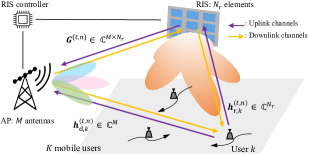
Figure 1: RIS assisted multiuser mobile communication system.

Consider a narrowband RIS-assisted multiuser multiple-input single-output (MU-MISO) system where $K$ single-antenna user equipment (UEs) are served by an access point (AP) with $M$ antennas. The RIS, equipped with $N_{r}$ passive elements, is placed between the AP and UEs to enable the reflection links as shown in Fig. 1. The RIS works cooperatively with the AP to control the phase of the reflected signals by tuning the phase shifters of each passive element through an RIS controller. We model the time-varying channel as a block-fading channel in discrete time, consisting of a sequence of fixed-length blocks. The channels are constant within the block and are correlated across the successive blocks. We further define a framing structure consisting of $N+1$ blocks per frame, and assume that channel variation is not significant within the frame so a fixed beamforming strategy can be used without incurring substantial performance loss. For the $n$-th block of the $t$-th frame, we use $\bm{G}^{(t,n)}\in\mathbb{C}^{M\times N_{r}}$, $\bm{h}_{\mathrm{d},k}^{(t,n)}\in\mathbb{C}^{M}$, and $\bm{h}_{\mathrm{r},k}^{(t,n)}\in\mathbb{C}^{N_{r}}$ to denote the channel matrix from the RIS to the AP, the channel vector from the UE $k$ to the AP, and the channel vector from the UE $k$ to the RIS, respectively.

In the $n$-th block of the $t$-th frame, let $s_{k}^{(t,n)}\in\mathbb{C}$ be the data symbol transmitted from the AP to the UE $k$, with $\mathbb{E}[|s_{k}^{(t,n)}|^{2}]=1$. The AP transmits $s_{k}^{(t,n)}$ to the UE $k$ through a beamforming vector $\bm{b}_{k}\in\mathbb{C}^{M}$, subject to a power constraint $\sum_{k=1}^{K}\|\bm{b}_{k}^{(t)}\|_{2}^{2}\leq P_{d}$, where $P_{d}$ is the downlink transmit power at the AP. We also denote $\bm{B}^{(t)}=[\bm{b}_{1}^{(t)},\dots,\bm{b}_{K}^{(t)}]\in\mathbb{C}^{M\times K}$ as the beamforming matrix at the AP in the $t$-th frame. Let $\bm{w}^{(t)}=[e^{j\theta_{1,t}},e^{j\theta_{2,t}},\dots,e^{j\theta_{N_{r},t}}]^{\sf{T}}\in\mathbb{C}^{N_{r}}$ be the downlink RIS reflection coefficients in the $t$-th frame, where $\theta_{i,t}\in[0,2\pi)$ is the phase shift of the $i$-th passive RIS element. Then, the signal $y_{k}^{(t,n)}\in\mathbb{C}$ received at the UE $k$ in the $n$-th block of the $t$-th frame can be expressed as:

$$y_{k}^{(t,n)}=\sum_{j=1}^{K}(\bm{A}_{k}^{(t,n)}\widetilde{\bm{w}}^{(t)})^{\sf{H}}\bm{b}_{j}^{(t)}s_{j}^{(t,n)}+z_{k}^{(t,n)}\ ,$$ (1)

where $\bm{A}_{k}^{(t,n)}\triangleq[\bm{h}_{\mathrm{d},k}^{(t,n)},\bm{G}^{(t,n)}\operatorname{diag}(\bm{h}_{\mathrm{r},k}^{(t,n)})]\in\mathbb{C}^{M\times(N_{r}+1)}$ is the combined channel between the AP and the UE $k$ in the $n$-th block of the $t$-th frame, $\widetilde{\bm{w}}^{(t)}\triangleq[1,(\bm{w}^{(t)})^{\sf{T}}]^{\sf{T}}\in\mathbb{C}^{N_{r}+1}$ is the effective RIS reflection coefficients, and $z_{k}^{(t,n)}\sim\mathcal{CN}(0,\sigma^{2}_{d})$ denotes the i.i.d. AWGN at the UE $k$. Therefore, the downlink achievable data rate $R_{k}^{(t,n)}$ for the UE $k$ in the $n$-th block of the $t$-th transmission frame can be expressed as:

$$R_{k}^{(t,n)}\!=\log\left(\!1\!+\!\frac{|(\bm{A}_{k}^{(t,n)}\widetilde{\bm{w}}^{(t)})^{\sf{H}}\bm{b}_{k}^{(t)}|^{2}}{\sum_{j=1,j\neq k}^{K}|(\bm{A}_{k}^{(t,n)}\widetilde{\bm{w}}^{(t)})^{\sf{H}}\bm{b}_{j}^{(t)}|^{2}\!+\!\sigma_{d}^{2}}\right)\!.$$ (2)

In this paper, our goal is to jointly optimize the beamforming matrix $\bm{B}^{(t)}$ and the RIS reflection coefficients $\bm{w}^{(t)}$ to establish $K$ reliable communication links between the AP and $K$ mobile UEs as well as to ensure fairness across the UEs. Accordingly, the optimization problem is formulated on a per-frame basis as:

$$(\mathrm{P}1):\;\;\;\mathop{\mathrm{maximize}}_{\bm{B}^{(t)},\ \bm{w}^{(t)}} \;\frac{1}{N}\sum_{n=1}^{N}\left(\min_{k}R_{k}^{(t,n)}\right)$$ (3)

$$\mathop{\mathrm{s.t.}} {}_{\mathop{}}\sum_{k=1}^{K}\|\bm{b}_{k}^{(t)}\|_{2}^{2}\leq P_{d}\ ,$$

$${}_{\mathop{}}\left\lvert[\bm{w}^{(t)}]_{i}\right\rvert=1,\ \forall i,t\ .$$

The optimization problem $(\mathrm{P}1)$ is a challenging nonconvex program. Moreover, solving problem $(\mathrm{P}1)$ requires the knowledge of the combined channel $\bm{A}_{k}^{(t,n)}$’s, which must be estimated. This paper assumes the system operates in time division duplex (TDD) mode, so we can leverage uplink-downlink channel reciprocity to acquire the instantaneous CSI from uplink pilots for downlink beamforming and for setting the RIS reflection coefficients.

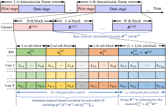
Figure 2: Frame structure of the proposed transmission protocol.

II-B Uplink Pilot Transmission Protocol

The uplink pilot transmission protocol is shown in Fig. 2, in which the mobile UEs send pilots to the AP in the $0$-th block of each transmission frame (also referred to as the pilot stage.) Moreover, this $0$-th block is divided into $L+1$ sub-blocks. The first $L$ sub-blocks consists of $\tau=K$ symbols; and the last sub-block consists of $\tau=\tau_{w}$ symbols, thus the pilot stage (i.e., the $0$-th block) has a total of $KL+\tau_{w}$ symbols.

Here, the pilots in the first $L$ sub-blocks serve to design the RIS reflection coefficients, while the pilots in the last sub-block are utilized for designing the AP beamformers. The pilot sequences $\bm{x}_{k}$ of the UEs are designed to be orthogonal to each other so that they can be decorrelated at the AP, i.e., $\bm{x}_{i}^{\sf{H}}\bm{x}_{j}=0$ if $i\neq j$ and $\bm{x}_{i}^{\sf{H}}\bm{x}_{i}=\tau P_{u}$, where $P_{u}$ is the uplink pilot transmission power, $\tau$ is the pilot length, and $i,j\in\{1,2,\dots,K\}$. The same pilots are sent repeatedly over the first $L$ sub-blocks to design the downlink transmission RIS coefficients in the current frame (as well as the RIS sensing coefficients in the next frame.) In the last sub-block, we fix the downlink transmission RIS coefficients then send $\tau_{w}$ additional pilots to estimate the effective low-dimensional channel.

A crucial observation here is that the pilots are received through the RIS reflection path. Thus, the RIS reflection coefficients are design parameters that can be set in each pilot stage. Here, we assume that the $L$ RIS reflection coefficients across the $L$ sub-blocks are designed together within each frame and adaptively across the frames, so that the UE-to-RIS and the RIS-to-AP channels are sensed in a sequential fashion in order to account for the historical channel observations. We refer to the set of $L$ RIS reflection coefficients in the pilot stage of each frame as the RIS sensing vectors.

In all $L+1$ sub-blocks, the AP decorrelates the received pilots in each sub-block by matching the pilot sequence for each UE. Let $\widehat{\bm{Y}}_{\ell}^{(t)}=[\widehat{\bm{y}}_{(\ell-1)\tau+1}^{(t)},\dots,\widehat{\bm{y}}_{\ell\tau}^{(t)}]\in\mathbb{C}^{M\times\tau}$ denote the received signal at the AP in the $\ell$-th sub-block of the pilot stage in the $t$-th frame. Let $\bm{v}^{(t)}_{\ell}\in\mathbb{C}^{N_{r}}$ denote the $\ell$-th sensing vector in the pilot stage of the $t$-th frame, we can express

$$\widehat{\bm{Y}}_{\ell}^{(t)}=\sum_{k=1}^{K}\bm{A}_{k}^{(t,0)}\widetilde{\bm{v}}^{(t)}_{\ell}\bm{x}_{k}^{\sf{H}}+\widehat{\bm{Z}}_{\ell}^{(t)}\ ,$$ (4)

where $\widetilde{\bm{v}}^{(t)}_{\ell}\triangleq[1,(\bm{v}^{(t)}_{\ell})^{\sf{T}}]^{\sf{T}}\in\mathbb{C}^{N_{r}+1}$ is the $\ell$-th effective sensing vector in the $t$-th frame and $\widehat{\bm{Z}}_{\ell}^{(t)}\in\mathbb{C}^{M\times\tau}$ is the sensing noise, whose columns are assumed to be independently distributed as $\mathcal{CN}(0,\sigma^{2}_{u}\bm{I})$. By the orthogonality of the pilots, we can form $\bar{\bm{y}}_{k,\ell}^{(t)}\in\mathbb{C}^{M}$, which is the contribution from the UE $k$ in the $\ell$-th sub-block of the pilot stage within the $t$-th frame [32, 24]:

$$\bar{\bm{y}}_{k,\ell}^{(t)}=\frac{1}{\tau P_{u}}\widehat{\bm{Y}}_{\ell}^{(t)}\bm{x}_{k}=\bm{A}_{k}^{(t,0)}\widetilde{\bm{v}}^{(t)}_{\ell}+\bar{\bm{z}}_{k,\ell}^{(t)}\ ,$$ (5)

where $\bar{\bm{z}}_{k,\ell}^{(t)}\!\triangleq\!\frac{1}{\tau P_{u}}\widehat{\bm{Z}}_{\ell}^{(t)}\bm{x}_{k}$. Denote $\bar{\bm{Y}}_{k}^{(t)}=[\bar{\bm{y}}_{k,1}^{(t)},\dots,\bar{\bm{y}}_{k,L}^{(t)}]\in\mathbb{C}^{M\times L}$ as the contribution from the UE $k$ across the first $L$ sub-blocks of the $t$-th frame, we can express $\bar{\bm{Y}}_{k}^{(t)}$ as:

$$\bar{\bm{Y}}_{k}^{(t)}\triangleq\bm{A}_{k}^{(t,0)}\bm{V}^{(t)}+\bar{\bm{Z}}_{k}^{(t)}\ ,$$ (6)

where $\bm{V}^{(t)}=[\widetilde{\bm{v}}^{(t)}_{1},\dots,\widetilde{\bm{v}}^{(t)}_{L}]\in\mathbb{C}^{(N_{r}+1)\times L}$ and $\bar{\bm{Z}}_{k}^{(t)}=[\bar{\bm{z}}_{k,1}^{(t)},\dots,\bar{\bm{z}}_{k,L}^{(t)}]\in\mathbb{C}^{M\times L}$.

Note that there are $(M+N_{r})K+MN_{r}$ unknown channel coefficients in $\bm{G}^{(t,0)}$, $\bm{h}_{r,k}^{(t,0)}$’s, and $\bm{h}_{d,k}^{(t,0)}$’s for $k=1,\dots,K$. Since the number of RIS elements $N_{r}$ is often very large (possibly hundreds), estimating the channels perfectly would lead to significant pilot overhead. It is therefore advantageous to bypass explicit channel estimation and to directly design the beamformers and the RIS reflection patterns based on the received pilots using a neural network [33].

Furthermore, the time-varying channels across different frames are often highly correlated, meaning that the historical channel information is valuable for predicting forthcoming channel states. It is therefore advantageous to use a sensing strategy that accounts for the historical channel observations across the frames, so it can focus on the region of interest to further save the pilot overhead, as described next.

III Active Sensing for Beam Tracking

To exploit the temporal correlations of the time-varying channel, this paper proposes an active sensing strategy for designing the RIS sensing vectors (in the first $L$ sub-blocks within the pilot stage of each frame) adaptively across frames based on the pilots received in previous frames. Within each frame, we also design the downlink data transmission RIS reflection coefficients after $L$ sub-blocks, then with $\tau_{w}$ additional pilots in the $(L+1)$-th sub-block, design the downlink AP beamformers. The detailed process is explained below.

In the pilot stage of the $t$-th transmission frame, the RIS sensing vectors $\{\bm{v}^{(t)}_{\ell}\}^{L}_{\ell=1}$ are designed based on the channel observations received prior to the $t$-th frame as:

$$\{\bm{v}^{(t)}_{\ell}\}^{L}_{\ell=1}=\mathcal{F}^{(t)}\left(\{\{\bar{\bm{Y}}_{k}^{(j)}\}_{k=1}^{K}\}_{j=1}^{t-1}\right)\ ,$$ (7)

where the elements of the output RIS sensing vector $\bm{v}^{(t)}_{\ell}$ should satisfy the unit modulus constraint, i.e., $|[\bm{v}^{(t)}_{\ell}]_{i}|=1$. Here, we refer to $\mathcal{F}^{(t)}:\mathbb{C}^{M\times LK(t-1)}\rightarrow\mathbb{C}^{N_{r}L}$ as the uplink active sensing scheme in the $t$-th frame. Since there are no channel observations before the $1$-st transmission frame, we let $\{\bm{v}^{(1)}_{\ell}\}^{L}_{\ell=1}=\mathcal{F}^{(1)}(\varnothing,\varnothing)$, where $\varnothing$ denotes that $\mathcal{F}^{(1)}(\cdot,\cdot)$ takes no input and outputs some random initial $\{\bm{v}^{(1)}_{\ell}\}^{L}_{\ell=1}$.

By utilizing the RIS sensing vectors $\{\bm{v}^{(t)}_{\ell}\}^{L}_{\ell=1}$, the AP collects a sequence of pilots as in (4) in the $t$-th transmission frame. Subsequently, the AP utilizes all the pilots received so far to design the downlink RIS reflection coefficients $\bm{w}^{(t)}$ for the subsequent data transmission within the $t$-th frame:

$$\bm{w}^{(t)}=\mathcal{G}^{(t)}\left(\{\{\bar{\bm{Y}}_{k}^{(j)}\}_{k=1}^{K}\}_{j=1}^{t}\right),$$ (8)

where the element of the output RIS reflection coefficients $\bm{w}^{(t)}$ should again satisfy the unit modulus constraint, i.e., $|[\bm{w}^{(t)}]_{i}|=1$. We also refer to $\mathcal{G}^{(t)}:\mathbb{C}^{M\times LKt}\rightarrow\mathbb{C}^{N_{r}}$ as the downlink beam alignment scheme in the $t$-th frame.

Next, we fix the RIS reflection coefficients as $\bm{w}^{(t)}$ and design the data transmission beamforming matrix $\bm{B}^{(t)}$ at the AP based on the pilot in the $(L+1)$-th sub-block. To reduce searching space, this paper leverages the following beamforming structure based on uplink-downlink duality [34]:

$$\bm{b}_{k}^{(t)}\!\!=\!\!\sqrt{p_{k}^{(t)}}\!\frac{(\bm{I}_{M}\!+\!\sum_{i\neq k}\frac{\lambda_{i}^{(t)}}{\sigma^{2}_{d}}\bm{h}_{c,i}^{(t,0)}(\bm{h}_{c,i}^{(t,0)})^{\sf{H}})^{-1}\bm{h}_{c,k}^{(t,0)}}{\|(\bm{I}_{M}\!+\!\sum_{i\neq k}\frac{\lambda_{i}^{(t)}}{\sigma^{2}_{d}}\bm{h}_{c,i}^{(t,0)}(\bm{h}_{c,i}^{(t,0)})^{\sf{H}})^{-1}\bm{h}_{c,k}^{(t,0)}\|_{2}},$$ (9)

where $\bm{h}_{c,k}^{(t,0)}\triangleq\bm{A}_{k}^{(t,0)}\widetilde{\bm{w}}^{(t)}\in\mathbb{C}^{M}$ denotes the low-dimensional effective channel between the AP and the UE $k$ in the pilot stage ($0$-th block) of the $t$-th frame. In (9), $p_{k}^{(t)}\geq 0$ and $\lambda_{k}^{(t)}\geq 0$ respectively represent for the primal downlink power and the virtual uplink power of the UE $k$ in the $t$-th frame, satisfying the power constraints $\sum_{k=1}^{K}p_{k}^{(t)}=\sum_{k=1}^{K}\lambda_{k}^{(t)}=P_{d}$. Accordingly, the beamforming vector design is equivalent to finding the optimal power allocations as follows:

$$\{\bm{p}^{(t)},\bm{\lambda}^{(t)}\}=\mathcal{H}^{(t)}\left(\{\bar{\bm{y}}_{k,L+1}^{(t)}\}_{k=1}^{K}\right),$$ (10)

where $\bm{p}^{(t)}\!\triangleq\![p_{1}^{(t)},\dots,p_{K}^{(t)}]^{\sf{T}}\!\in\!\mathbb{R}^{K}$, $\bm{\lambda}^{(t)}\!\triangleq\![\lambda_{1}^{(t)},\dots,\lambda_{K}^{(t)}]^{\sf{T}}\!\in\mathbb{R}^{K}$, and $\mathcal{H}^{(t)}:\mathbb{C}^{MK}\rightarrow\mathbb{R}^{K\times K}$ is the downlink power allocation scheme in the $t$-th frame.

In (9), we note that the effective channel $\bm{h}_{c,k}^{(t,0)}$ is needed to design the beamforming vectors. Here, since $\bm{h}_{c,k}^{(t,0)}$ is a low-dimensional channel vector, its estimation is straightforward when the RIS reflection coefficients $\widetilde{\bm{w}}^{(t)}$ are fixed. Specifically, this paper simply estimates $\bm{h}_{c,k}^{(t,0)}$ based on the pilot in the $(L+1)$-th sub-block as follows. The decorrelated received pilot $\bar{\bm{y}}_{k,L+1}^{(t)}$ from the UE $k$ in the $(L+1)$-th sub-block is $\bar{\bm{y}}_{k,L+1}^{(t)}=\bm{A}_{k}^{(t,0)}\widetilde{\bm{w}}^{(t)}+\bar{\bm{z}}_{k,L+1}^{(t)}\triangleq\bm{h}_{c,k}^{(t,0)}+\bar{\bm{z}}_{k,L+1}^{(t)}$. So approximately, the effective low-dimensional channel $\check{\bm{h}}_{c,k}^{(t,0)}\in\mathbb{C}^{M}$ is simply:

$$\check{\bm{h}}_{c,k}^{(t,0)}=\bar{\bm{y}}_{k,L+1}^{(t)}\ .$$ (11)

We can now formulate the multiuser beam tracking problem for maximizing the minimum downlink user rate as that of designing the uplink active sensing scheme $\mathcal{F}^{(t)}$, the downlink beam alignment scheme $\mathcal{G}^{(t)}$, and the downlink power allocation scheme $\mathcal{H}^{(t)}$ to maximize:

$$\begin{array}[]{ll}(\mathrm{P}2)\!:\;\;\underset{\begin{subarray}{c}\mathcal{F}^{(t)}(\cdot),\ \mathcal{G}^{(t)}(\cdot),\\ \mathcal{H}^{(t)}(\cdot)\end{subarray}}{\operatorname{maximize}}&\mathbb{E}\left[\displaystyle\frac{1}{N}\sum_{n=1}^{N}\left(\min_{k}R_{k}^{(t,n)}\right)\right]\\ \ \ \ \ \ \ \ \ \ \ \ \ \ \ \ \ \mathrm{s.t.}&\eqref{eq: UL sensing scheme},\ \eqref{eq: downlink beam alignment scheme},\ \eqref{beamforming structure},\ \eqref{eq: downlink power allocation scheme},\ \eqref{eq: LS}\ ,\end{array}$$ (12)

where the expectation is taken over the channel and noise distributions, and $N$ is the number of data blocks in every transmission frame. The objective function is chosen to ensure that all UEs meet a downlink rate constraint during all $N$ blocks of data transmissions.

Analytically solving this variational optimization problem $(\mathrm{P}2)$ is challenging, because it involves a joint optimization over the high-dimensional mappings $\mathcal{F}^{(t)}$, $\mathcal{G}^{(t)}$, and $\mathcal{H}^{(t)}$. Moreover, since the input dimensions of the functions $\mathcal{F}^{(t)}$, $\mathcal{G}^{(t)}$, and $\mathcal{H}^{(t)}$ increase with the number of tracking frames, finding a scalable solution analytically is nearly impossible.

To address the challenge of solving problem $(\mathrm{P}2)$, we propose to utilize deep neural network as a powerful function approximator [35] to parameterize the functions $\mathcal{F}^{(t)}$, $\mathcal{G}^{(t)}$, and $\mathcal{H}^{(t)}$. In this way, the computational complexity of the optimization is transferred to the neural network training process [33]. The key is to identify a neural network architecture capable of summarizing historical channel information across different frames in designing an optimal sensing strategy for beam tracking, as well as in performing effective interference management within each frame.

IV Learning-Based Active Sensing Framework for Multiuser Beam Tracking

This paper proposes a learning-based active sensing framework that optimizes both the uplink channel sensing and downlink data transmission strategies for effective multiuser beam tracking. Specifically, we employ a GNN to model the spatial relation between the UEs and the RIS, while leveraging the graphic structure to efficiently manage interference among the UEs. Furthermore, we utilize a LSTM-based RNN to capture the temporal correlations in the channel dynamics in order to exploit the historical channel information in designing active sensing and beam tracking strategies.

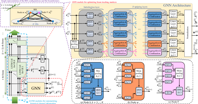
Figure 3: Overall graph neural network architecture with an initialization layer, $D$ updating layers, and a final normalization layer.

IV-A GNN for Interference Management

In an RIS-assisted multiuser mobile communication systems, a primary challenge lies in managing the interference among UEs. Interference management requires coordination between the downlink beamformers and the RIS reflection coefficients, which need to be designed based on the received pilots through appropriate RIS sensing vectors.

This paper proposes to use a GNN to map the effective CSI information to the optimized uplink sensing and downlink reflection coefficients at the RIS, as well as the downlink power allocations at the AP for each transmission frame. A key motivation for employing a GNN is that it captures the permutation invariant and equivariant properties of the beam tracking problem. Specifically, the optimal RIS reflection coefficients should remain unchanged regardless of user ordering (i.e., permutation invariant). Likewise, any permutation of user index labels should permute the AP beamformers correspondingly (i.e., permutation equivariant). These properties are difficult to learn by a fully connected neural network, but are embedded in the architecture of a GNN [36] and have been successfully applied in the RIS setting [24].

The spatial relation among the UEs and the RIS are modeled based on graph representations of the RIS configurations and AP beamformers as shown in Fig. 3. The graph consists of $K+2$ nodes, with nodes $1$ to $K$ correspond to the power allocations for UE $1$ through UE $K$, and the nodes labeled $V$ and $w$ correspond to the uplink sensing and downlink reflection coefficients at the RIS, respectively. Each node $\xi$, $\xi\in\{w,V,1,\dots K\}$, is associated with a representation vector denoted by $\bm{s}^{(t)}_{\xi}$. Specifically, the vector $\bm{s}^{(t)}_{w}$ is used for designing the downlink RIS reflection coefficients $\bm{w}^{(t)}$, the vector $\bm{s}^{(t)}_{V}$ is used for designing the RIS sensing vectors $\{\bm{v}^{(t+1)}_{\ell}\}^{L}_{\ell=1}$, and the vector $\bm{s}^{(t)}_{k}$ is used for designing the power allocations $\{p_{k}^{(t)},\lambda_{k}^{(t)}\}$ of the beamformer $\bm{b}^{(t)}_{k}$. We design the graph with user nodes $1$ to $K$ being fully connected, and establish edges from RIS nodes $V$ and $w$ to all user nodes, respectively. Here, the RIS nodes $V$ and $w$ have different representation vectors, because sensing and data transmission have very different functionalities.

The overall GNN aims to learn the graph representation vector $\bm{s}^{(t)}_{\xi}$’s through an initialization layer, $D$ updating layers, and a final layer that includes normalization. As shown in Fig. 3, the GNN first encodes all the useful information about each node in the $t$-th transmission frame into a corresponding representation vector $\bm{s}^{(t)}_{\xi,0}$’s according to:

$$\bm{s}^{(t)}_{k,0} =f_{1}(\bm{c}^{(t)}_{k})\ ,\ k=1,\dots,K\ ,$$ (13a)

$$\bm{s}^{(t)}_{w,0} =f_{2}(\psi_{1}(\bm{c}^{(t)}_{1},\dots,\bm{c}^{(t)}_{K}))\ ,$$ (13b)

$$\bm{s}^{(t)}_{V,0} =f_{3}(\psi_{1}(\bm{c}^{(t)}_{1},\dots,\bm{c}^{(t)}_{K}))\ ,$$ (13c)

where $\psi_{1}(\cdot)$ is the element-wise mean pooling function, and $\bm{c}^{(t)}_{k}$’s are the state information vectors that contain all the useful channel information of the corresponding mobile UEs in the $t$-th frame. Here, $f_{1}(\cdot)$, $f_{2}(\cdot)$, and $f_{3}(\cdot)$ represent fully connected neural networks with the rectified linear unit (ReLU) activation function employed in all the dense layers.

To capture the spatial structure between the RIS and UEs, the initial graph representation vector $\bm{s}^{(t)}_{\xi,0}$’s undergo $D$ iterations of updates, each utilizing the output of the preceding layer as input. More specifically, the updates for the RIS node $w$ and $V$ incorporate their current representations as well as the representations of all UE nodes, while the representation vector of the UE node $k$ is updated based on its own prior representation and the representations of all other nodes in the network. These update procedures maintain the GNN’s permutation invariance and equivariance, and therefore allows more efficient training. The updating rules of the $d$-th updating layer are given as:

$$\bm{s}^{(t)}_{k,d+1} =f_{5}(\bm{s}^{(t)}_{k,d},f_{V}(\bm{s}^{(t)}_{V,d}),f_{w}(\bm{s}^{(t)}_{w,d}),\psi_{2}(\{f_{4}(\bm{s}^{(t)}_{\xi,d})\}_{\forall\xi\neq k})),$$ (14a)

$$\bm{s}^{(t)}_{w,d+1} =f_{7}(f_{w}(\bm{s}^{(t)}_{w,d}),\psi_{1}(f_{6}(\bm{s}^{(t)}_{1,d}),\dots,f_{6}(\bm{s}^{(t)}_{K,d})),$$ (14b)

$$\bm{s}^{(t)}_{V,d+1} =f_{9}(f_{V}(\bm{s}^{(t)}_{V,d}),\psi_{1}(f_{8}(\bm{s}^{(t)}_{1,d}),\dots,f_{8}(\bm{s}^{(t)}_{K,d})).$$ (14c)

Here, $\psi_{2}(\cdot)$ is the element-wise max pooling function, while $f_{4}(\cdot),f_{5}(\cdot),f_{6}(\cdot),f_{7}(\cdot),f_{8}(\cdot),f_{9}(\cdot),f_{w}(\cdot),f_{V}(\cdot)$ are fully connected neural networks with ReLU activation function applied in each of their dense layers.

After $D$ layers of iteration, the updated representation vector $\bm{s}^{(t)}_{\xi,D}$’s would contain sufficient information to design the beam tracking matrices. To obtain the correct output dimensions, we pass $\bm{s}^{(t)}_{k,D}$’s, $\bm{s}^{(t)}_{w,D}$, and $\bm{s}^{(t)}_{V,D}$ through linear layers $g_{1}(\cdot),g_{2}(\cdot),g_{3}(\cdot)$ with $2K$, $2N_{r}$, and $2N_{r}L$ fully connected units, respectively. Specifically, $\bm{s}^{(t)}_{k,D+1}=g_{1}(\bm{s}^{(t)}_{k,D})\in\mathbb{R}^{2K}$, $\bm{s}^{(t)}_{w,D+1}=g_{2}(\bm{s}^{(t)}_{w,D})\in\mathbb{R}^{2N_{r}}$, and $\bm{s}^{(t)}_{V,D+1}=g_{3}(\bm{s}^{(t)}_{V,D})\in\mathbb{R}^{2N_{r}L}$. The final representation vector $\bm{s}^{(t)}_{\xi,D+1}$’s are then normalized to produce the RIS sensing vectors $\{\bm{v}^{(t+1)}_{\ell}\}^{L}_{\ell=1}$, downlink RIS reflection coefficients $\bm{w}^{(t)}$, and power allocations $\{\bm{p}^{(t)},\bm{\lambda}^{(t)}\}$, respectively, while ensuring that the unit modulus constraints on $\bm{w}^{(t)}$, $\bm{v}_{\ell}^{(t+1)}$’s and the power constraints on $\{\bm{p}^{(t)},\bm{\lambda}^{(t)}\}$ are satisfied.

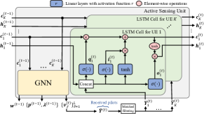
Figure 4: Active sensing unit for multiuser beam tracking with RIS.

IV-B LSTM for Exploiting Temporal Channel Correlation

This paper proposes to use an LSTM-based RNN to capture the temporal correlations of the time-varying channel by automatically summarizing the channel information into state information vector $\bm{c}^{(t)}_{k}$’s in (13), which are further processed by the GNN to design the beam tracking strategies. As shown in Fig. 4, $K$ copies of the LTSM cells with shared weights are deployed to summarize the state information for the $K$ mobile UEs, respectively. In the $t$-th frame, the $k$-th LSTM cell takes new pilots $\bar{\bm{Y}}_{k}^{(t)}$ from UE $k$ to update its hidden state vector $\bm{h}_{k}^{(t)}$ and cell state vector $\bm{c}_{k}^{(t)}$ according to [7]:

$$\bm{c}^{(t)}_{k} =\bm{q}_{k}^{(t)}\circ\bm{c}_{k}^{(t-1)}+\bm{i}_{k}^{(t)}\circ\tanh(\bm{u}_{c}(\bar{\bm{Y}}_{k}^{(t)})+\bm{w}_{c}(\bm{h}_{k}^{(t-1)})),$$ (15a)

$$\bm{h}_{k}^{(t)} =\bm{o}_{k}^{(t)}\circ\tanh(\bm{c}_{k}^{(t)})\ ,$$ (15b)

where $\bm{q}_{k}^{(t)}$, $\bm{i}_{k}^{(t)}$, and $\bm{o}_{k}^{(t)}$ are the activation vectors of the forget gate, input gate and output gate within the $k$-th LSTM cell, respectively. The updating rules for different gates are given as $\bm{r}_{k}^{(t)}=\sigma(\bm{u}_{r}(\bar{\bm{Y}}_{k}^{(t)})+\bm{w}_{r}(\bm{h}_{k}^{(t-1)}))$, where $r\in\{q,i,o\}$, and $\sigma(\cdot)$ is the element-wise sigmoid function. Here, $\bm{u}_{c}$, $\bm{u}_{q}$, $\bm{u}_{i}$, $\bm{u}_{o}$, $\bm{w}_{c}$, $\bm{w}_{q}$, $\bm{w}_{i}$, and $\bm{w}_{o}$ are fully connected layers, with the weights of each being shared across $K$ LSTM cells.

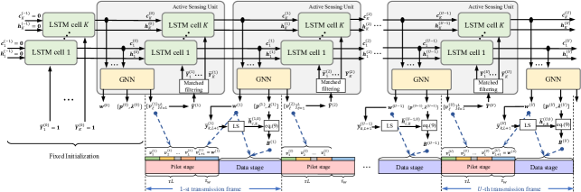
Figure 5: Proposed active sensing framework for multiuser beam tracking with RIS. During the training phase, we concatenated $U$ active sensing units correspond to $U$ transmission frames. Once trained and deployed, we reuse the active sensing units for a potentially infinite number of transmission frames.

IV-C Active Sensing Framework for Beam Tracking

The overall active sensing framework is shown in Fig. 5. It works as follows.

IV-C1 RIS Sensing Vector Design

In the pilot stage of the $(t-1)$-th frame, the LSTM cell state $\bm{c}_{k}^{(t-1)}$’s that encapsulate the temporal channel correlations for the $K$ mobile UEs based on the previous frames are fed into a GNN. The GNN then outputs the RIS sensing vectors $\{\bm{v}^{(t)}_{\ell}\}^{L}_{\ell=1}$ for the next round of CSI acquisition (i.e., pilot stage of the $t$-th frame). We observe empirically that it is also possible to replace the LSTM cell state $\bm{c}_{k}^{(t-1)}$ with the hidden state $\bm{h}_{k}^{(t-1)}$ as the GNN input.

IV-C2 State Vector Update

In the $t$-th frame, $K$ LSTM cells with shared weights take in the most recent channel observation $\bar{\bm{Y}}_{k}^{(t)}$’s, alongside the preceding cell state $\bm{c}_{k}^{(t-1)}$’s and hidden state $\bm{h}_{k}^{(t-1)}$’s, to generate the new cell states $\bm{c}_{k}^{(t)}$’s and hidden state $\bm{h}_{k}^{(t)}$’s. By convention, we initialize $\bm{c}_{k}^{(-1)}=\bm{h}_{k}^{(-1)}=\bm{0}$, and $\bar{\bm{Y}}_{k}^{(0)}=\bm{1}$ for all $k$ in $\{0,\dots,K\}$.

IV-C3 Downlink Beam Alignment

Utilizing the updated LSTM cell state $\bm{c}_{k}^{(t)}$’s as input, the proposed GNN computes the downlink RIS reflection coefficients $\bm{w}^{(t)}$ and power allocations $\{\bm{p}^{(t)},\bm{\lambda}^{(t)}\}$. The AP then estimates the effective low-dimensional channel $\bm{h}_{c,k}^{(t,0)}$’s based on the additional $\tau_{w}$ pilot symbols transmitted via the reflection of the $(L+1)$-th RIS sensing vector $\bm{v}_{L+1}^{(t)}=\bm{w}^{(t)}$. With the estimated low-dimensional channel $\check{\bm{h}}_{c,k}^{(t,0)}$ and designed power allocations $\{\bm{p}^{(t)},\bm{\lambda}^{(t)}\}$, the downlink beamforming vector $\bm{b}^{(t)}_{k}$’s for subsequent data transmissions are computed via (9).

IV-D Neural Network Training and Inference

The active sensing units are concatenated to form a deep neural network as shown in Fig. 5, with each unit corresponding to a transmission frame. The neural network weights are tied together across the stages. By training the concatenated neural network, the active sensing unit is able to explore the temporal channel correlation from the input pilot sequence. The proposed architecture is trained offline in an unsupervised fashion. Specifically, we employ Adam optimizer [37] to minimize the negative of the average minimum downlink rate over $U$ frames as $-\frac{1}{U}\sum_{t=1}^{U}\mathbb{E}[\frac{1}{N}\sum_{n=1}^{N}(\min_{k}R_{k}^{(t,n)})]$, where the expectation is approximated by the empirical average over the training set. In this way, the uplink active sensing scheme $\mathcal{F}^{(t)}$, the downlink beam alignment scheme $\mathcal{G}^{(t)}$, and the downlink power allocation scheme $\mathcal{H}^{(t)}$ are jointly designed to optimize the beam tracking performance. In practice, we choose the number of the concatenated active sensing units $U$ to be sufficiently large so that the temporal correlations of the time-varying channel can be learned through the periodically received pilots. Once the neural network is trained, the trained active sensing unit can be reused for a potentially infinite number of frames, since the LSTM cell learns to keep updating the channel information based on the latest received pilots.

In the simulations, we observe that it is possible to further improve the performance of directly using the power allocations $\{\bm{p}^{(t)},\bm{\lambda}^{(t)}\}$ designed by neural network. This is primarily because the proposed active sensing framework only has moderate size of the hidden neurons, which restricts its expressive capacity. It is possible to adopt a refined approach using the fact that the effective low-dimensional channel $\bm{h}_{c,k}^{(t,0)}$’s can be easily estimated according to (11). By employing a fixed-point iterations method [38, 39] which takes the estimated $\check{\bm{h}}_{c,k}^{(t,0)}$’s as input, we can analytically determine the optimal power allocations. This method allows for a more precise adjustment of power allocations, ensuring that the beamforming vectors computed therefrom are better optimized.

More specifically, the optimal power allocation $\bm{\lambda}^{(t)}_{*}$ is the unique positive solution of the following fixed-point equation:

$$[\bm{\lambda}^{(t)}_{*}]_{k}=\frac{\tau^{(t)}_{*}}{f(\bm{\lambda}^{(t)}_{*},\check{\bm{h}}_{c,k}^{(t,0)},\{\check{\bm{h}}_{c,i}^{(t,0)}\}_{\forall i\neq k})}$$ (16)

$$\triangleq\frac{\tau^{(t)}_{*}}{(\check{\bm{h}}_{c,k}^{(t,0)})^{\sf{H}}(\sum_{i\neq k}[\bm{\lambda}^{(t)}_{*}]_{i}\check{\bm{h}}_{c,i}^{(t,0)}(\check{\bm{h}}_{c,i}^{(t,0)})^{\sf{H}}+\sigma_{d}^{2}\bm{I}_{M})^{-1}\check{\bm{h}}_{c,k}^{(t,0)}}\ ,$$

where $\tau^{(t)}_{*}\!=\!P_{d}/\sum_{k=1}^{K}(f(\bm{\lambda}^{(t)}_{*},\check{\bm{h}}_{c,k}^{(t,0)},\{\check{\bm{h}}_{c,i}^{(t,0)}\}_{\forall i\neq k}))^{-1}$.

Further, the optimal power allocation $\bm{p}^{(t)}_{*}$ is obtained as:

$$\bm{p}^{(t)}_{*}=(\bm{I}_{K}-\tau^{(t)}_{*}\bm{D}^{(t)}\bm{F}^{(t)})^{-1}\tau^{(t)}_{*}\sigma_{d}^{2}\bm{D}^{(t)}\bm{1}_{K}\ ,$$ (17)

where $\bm{D}^{(t)}=\text{diag}(\frac{1}{|(\check{\bm{h}}_{c,1}^{(t,0)})^{\sf{H}}\widetilde{\bm{b}}^{(t)}_{1}|^{2}},\dots,\frac{1}{|(\check{\bm{h}}_{c,K}^{(t,0)})^{\sf{H}}\widetilde{\bm{b}}^{(t)}_{K}|^{2}})$ and $[\bm{F}^{(t)}]_{k,i}=1/|(\check{\bm{h}}_{c,k}^{(t,0)})^{\sf{H}}\widetilde{\bm{b}}^{(t)}_{i}|^{2}$, if $k\neq i$ and $0$ otherwise. Here, $\widetilde{\bm{b}}^{(t)}_{k}$’s denote the beamforming directions which can be computed based on $\bm{\lambda}^{(t)}_{*}$ and $\check{\bm{h}}_{c,k}^{(t,0)}$’s via (9).

Note however, in order to preserve the differentiability of gradients during back-propagation, we cannot employ the fixed-point iterations for computing power allocations in the neural network’s training phase. Only in the inference phase of the proposed active sensing framework, we replace the power allocations $\{\bm{p}^{(t)},\bm{\lambda}^{(t)}\}$ designed by the GNN with $\{\bm{p}^{(t)}_{*},\bm{\lambda}^{(t)}_{*}\}$ analytically determined through fixed-point iterations to obtain the best performance.

V Numerical Results and Interpretations

V-A Simulation Setup

We consider an RIS-assisted MU-MISO communication system as illustrated in Fig. 8, consisting of an AP with $8$ antennas and an RIS with $100$ passive elements. In the Cartesian coordinate system shown in Fig. 8, the $(x,y,z)$-coordinates of the AP and the RIS are $(100\text{m},-100\text{m},0\text{m})$ and $(0\text{m},0\text{m},0\text{m})$, respectively. We assume that the RIS is equipped with a $10\times 10$ uniform rectangular array placed on the $(y,z)$-plane, and the AP has a uniform linear array parallel to the $x$-axis. The system is assumed to operate at a carrier frequency $f_{c}=1\text{GHz}$ with $10$MHz bandwidth. The uplink pilot transmit power $P_{u}$ and the downlink data transmit power $P_{d}$ are set to be $5$dBm and $10$dBm, and the noise spectrum density at the AP and UE are set to be $N_{0,u}=-154$dBm/Hz and $N_{0,d}=-160$dBm/Hz, respectively.

V-A1 UE Mobility Model

As shown in Fig. 8, there are $K=3$ mobile UEs located within a rectangular service area $[5\text{m},45\text{m}]\times[-35\text{m},35\text{m}]$ on the $(x,y)$-plane, with their $z$-coordinates fixed as $-20\text{m}$. Furthermore, as illustrated in Fig. 8, the $(x,y)$-coordinates of the mobile UE $k$ in the $(i+1)$-th time block are determined as:

$$[x_{k}^{(i+1)},y_{k}^{(i+1)}]^{\sf{T}}=[x_{k}^{(i)},y_{k}^{(i)}]^{\sf{T}}+[\lambda\cos\gamma_{k}^{(i)},\lambda\sin\gamma_{k}^{(i)}]^{\sf{T}}\!,$$ (18)

where $\gamma_{k}^{(i)}$ denotes the moving direction of the UE $k$ in the $i$-th time block and $\lambda$ denotes the UE displacement per block. Here, the initial position of the UEs is uniformly distributed within the service area, i.e., $x_{k}^{(1)}\sim\mathcal{U}(5\text{m},45\text{m})$ and $y_{k}^{(1)}\sim\mathcal{U}(-35\text{m},35\text{m})$. To model practical trajectories of the mobile UEs, we assume that $\gamma_{k}^{(i)}$ is updated at each block as $\gamma_{k}^{(i+1)}=\gamma_{k}^{(i)}+\triangle\gamma$, where the initial moving direction $\gamma_{k}^{(1)}\sim\mathcal{U}(0,2\pi)$ and $\triangle\gamma\sim\mathcal{U}(-10^{\circ},10^{\circ})$. We further assume that the mobile UEs move at a constant speed of $v_{\text{UE}}=10\text{m/s}$, which results in a maximum Doppler frequency $f_{max}=v_{\text{UE}}f_{c}/c=33.3\text{Hz}$ with $c=3\times 10^{8}\text{m/s}$ as the speed of light. The UE displacement per block is then calculated as $\lambda=v_{\text{UE}}T_{b}=v_{\text{UE}}/2f_{max}=0.15\text{m}$, where $T_{b}=1/2f_{max}$ is the duration of each block. The mobile UEs are restricted to a $40\text{m}\times 70\text{m}$ service area. If a UE crosses this boundary, its coordinates and movement direction are mirrored back into the area, as shown in Fig. 8.

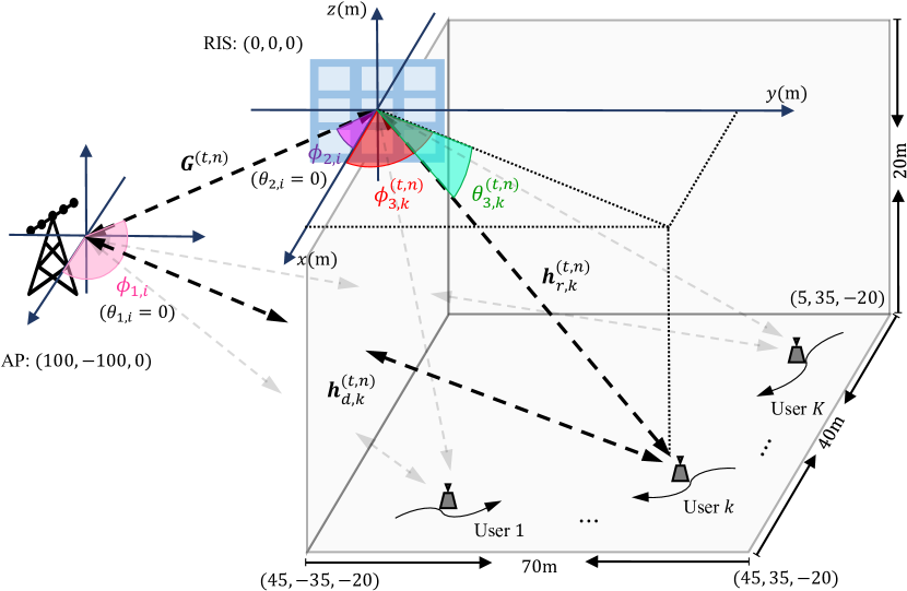
Figure 6: System geometries for simulations.

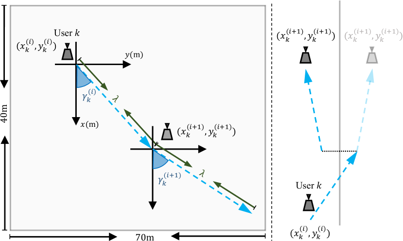
Figure 7: Illustration of the UE’s mobility model.

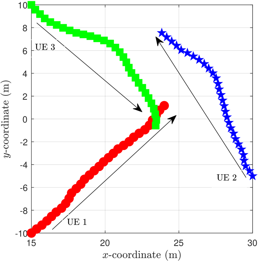
Figure 8: Trajectories of UEs.

V-A2 Channel Model

In the $n$-th block of the $t$-th transmission frame, we assume that the channels from the AP to the mobile UEs are modeled by the Rayleigh fading as:

$$\bm{h}_{d,k}^{(t,n)}=\beta_{d,k}^{(t,n)}\widetilde{\bm{h}}_{d,k}^{(t,n)}\ ,$$ (19)

where $\beta_{d,k}^{(t,n)}$ denotes the path-loss of the direct link between the AP and the UE $k$ modeled in (dB) as $32+43.3\log(l_{d,k}^{(t,n)})$, where $l_{d,k}^{(t,n)}$ is the distance of the direct link from the AP to the UE $k$. The variation of the entries of the non-line-of-sight (NLOS) components of the direct link $[\widetilde{\bm{h}}_{d,k}^{(t,n)}]_{i}$ is modeled by the stationary Gauss-Markov process as follows [14]:

$$\left\{\begin{aligned} {}_{i}&=\rho[\widetilde{\bm{h}}_{d,k}^{(t,n-1)}]_{i}+\sqrt{1-\rho^{2}}\mu^{(t,n-1)},2\leq n\leq N,\\ [\widetilde{\bm{h}}_{d,k}^{(t,n)}]_{i}&=\rho[\widetilde{\bm{h}}_{d,k}^{(t-1,N)}]_{i}+\sqrt{1-\rho^{2}}\mu^{(t-1,N)}\ ,\ n=1\ ,\end{aligned}\right.$$ (20)

where the correlation coefficient $\rho=0.9995$, perturbation term $\mu^{(k,n)}\sim\mathcal{CN}(0,1)$, and $[\widetilde{\bm{h}}_{d,k}^{(1,1)}]_{i}\sim\mathcal{CN}(0,1)$. We assume that the RIS is deployed at a location where multiple paths exist between the AP and the RIS, and a LOS channel exists between the RIS and each mobile UE. More specifically, the AP-RIS link $\bm{G}^{(t,n)}$ and the RIS-UE link $\bm{h}_{r,k}^{(t,n)}$’s follow the Rician fading model as:

$$\bm{G}^{(t,n)}=\beta_{G}^{(t,n)}(\sqrt{\varepsilon/(1+\varepsilon)}\ \sum_{i}^{N_{G}}\widehat{\bm{G}}_{i}+\sqrt{1/(1+\varepsilon)}\ \widetilde{\bm{G}}^{(t,n)}),$$ (21)

$$\bm{h}_{r,k}^{(t,n)}=\beta_{r,k}^{(t,n)}(\sqrt{\varepsilon/(1+\varepsilon)}\ \widehat{\bm{h}}_{r,k}^{(t,n)}+\sqrt{1/(1+\varepsilon)}\ \widetilde{\bm{h}}_{r,k}^{(t,n)}),$$ (22)

where $N_{G}$ is the number of paths between the AP and RIS, and $\varepsilon$ is the Rician factor which is set to be $10$. The path loss (in dB) of the AP-RIS link $\beta_{G}$ and the RIS-UE link $\beta_{r}^{(t,n)}$ are modeled as $28+16.9\log(l_{G})$ and $28+16.9\log(l_{r}^{(t,n)})$, respectively, where $l_{G}$ and $l_{r}^{(t,n)}$ are the distance of the corresponding links. Similar to (20), the distribution of the entries of the NLOS components of the AP-RIS link $[\widetilde{\bm{G}}^{(t,n)}]_{ij}$ and the RIS-UE link $[\widetilde{\bm{h}}_{r,k}^{(t,n)}]_{i}$’s are modeled by the same stationary Gauss-Markov process, with $[\widetilde{\bm{G}}^{(1,1)}]_{ij}\sim\mathcal{CN}(0,1)$ and $[\widetilde{\bm{h}}_{r,k}^{(1,1)}]_{i}\sim\mathcal{CN}(0,1)$.

The LOS part of the RIS-UE link $\widehat{\bm{h}}_{r,k}^{(t,n)}$ is a function of the UE/RIS locations. Specifically, let $\theta_{3,k}^{(t,n)}$, $\phi_{3,k}^{(t,n)}$ denote the elevation and azimuth angle of arrivals (AoAs) from the UE $k$ to the RIS at the $n$-th block of the $t$-th frame, as shown in Fig. 8. We can write $\widehat{\bm{h}}_{r,k}^{(t,n)}=\bm{a}_{\text{RIS}}(\theta_{3,k}^{(t,n)},\phi_{3,k}^{(t,n)})$, where the $u$-th element of the steering vector at RIS is given as [24]:

$${[\bm{a}_{\text{RIS}}(\theta_{3,k}^{(t,n)},\phi_{3,k}^{(t,n)})]_{u}}$$ (23)

$$=e^{j\frac{2\pi d_{\text{RIS}}}{\lambda_{c}}\{i_{1}(u,v)\sin(\phi_{3,k}^{(t,n)})\cos(\theta_{3,k}^{(t,n)})+i_{2}(u,v)\sin(\theta_{3,k}^{(t,n)})\}}.$$

Here, $\lambda_{c}$ is the carrier wavelength, $d_{\text{RIS}}$ is the distance between two adjacent RIS elements, $i_{1}(u,v)=\bmod(u-1,v)$, and $i_{2}(u,v)=\lfloor\frac{u-1}{v}\rfloor$, where $v$ is the number of columns of the RIS. Without loss of generality, we set $d_{\text{RIS}}=\lambda_{c}/2$ and $v=10$ in simulations. Similarly, let $\phi_{2,i}$ and $\phi_{1,i}$ denote the $i$-th azimuth angle of departure (AoD) and azimuth AoA from the RIS to the AP, corresponding to the $i$-th path $\widehat{\bm{G}}_{i}$ between the AP and the RIS. Then we can write $\widehat{\bm{G}}_{i}=\bm{a}_{\text{AP}}(\phi_{1,i})\bm{a}_{\text{RIS}}(\theta_{2,i},\phi_{2,i})^{\sf{H}}$, where $\theta_{2,i}=0$ as shown in Fig. 8 and the steering vector of the AP is given by:

$$\bm{a}_{\text{AP}}(\phi_{1,i})=[1,\cdots,e^{j\frac{2\pi(M-1)d_{\text{AP}}}{\lambda_{c}}\cos\left(\phi_{1,i}\right)}]^{\sf{T}}.$$ (24)

Here, $d_{\text{AP}}$ denotes the distance between two adjacent antenna elements. In simulations, we set $d_{\text{AP}}=\lambda_{c}/2$ and generate the AoAs/AoDs according to uniform distributions, i.e., $\phi_{1,i}\sim\mathcal{U}(0,2\pi)$ and $\phi_{1,i}\sim\mathcal{U}(-\pi/2,0)$.

V-B Implementation Details

The proposed active sensing framework is implemented on Tensorflow [40]. For the LSTM cells, the dimensions of hidden state $\bm{h}_{k}^{(t)}$’s, cell state $\bm{c}_{k}^{(t)}$’s, and hidden layers $\bm{u}_{c}$, $\bm{u}_{q}$, $\bm{u}_{i}$, $\bm{u}_{o}$, $\bm{w}_{c}$, $\bm{w}_{q}$, $\bm{w}_{i}$, $\bm{w}_{o}$ are set to be $512$. We adopt a GNN with $D=2$ updating layers. Within the GNN architecture, the DNNs $f_{1}(\cdot)$, $f_{2}(\cdot)$, and $f_{3}(\cdot)$ are of size $512\times 1024\times 512$, and the size of DNNs $f_{4}(\cdot)$, $f_{5}(\cdot)$, $f_{6}(\cdot)$, $f_{7}(\cdot)$, $f_{8}(\cdot)$, $f_{9}(\cdot)$, $f_{w}(\cdot)$, $f_{V}(\cdot)$ are $512\times 512\times 512$. We concatenate $U=20$ active sensing units to train the proposed framework. In each training epoch, the neural network samples $6400$ training data including random channel and noise realizations. We terminate the training process if the validation loss does not decrease over $30$ consecutive training epochs. An instance of trajectories for $K=3$ mobile UEs is shown in Fig. 8.

We assume there are $N_{G}=8$ paths between the AP and RIS. Each transmission frame contains $N=3$ blocks. In the pilot stage (the $0$-th block) of each frame, there are $4$ sub-blocks, i.e., $L=3$. The effective downlink channel $\bm{h}_{c,k}^{(t,0)}$’s are estimated in the $4$-th sub-block with $\tau_{w}=10$ pilots.

V-C Benchmark Methods

BCD with Perfect CSI [3]

Given the perfect CSI of the channel $\bm{G}^{(t,1)}$, $\bm{h}_{\mathrm{d},k}^{(t,1)}$’s, and $\bm{h}_{\mathrm{r},k}^{(t,1)}$’s, we can find a performance benchmark for the proposed active sensing framework by solving the following optimization problem:

$$(\bm{B}^{(t)}_{*},\bm{w}^{(t)}_{*})=\mathrm{argmax}_{\bm{B}^{(t)},\bm{w}^{(t)}}\min_{k}\{R_{k}^{(t,1)}\}\ ,$$ (P3)

subject to $\sum_{k}\|\bm{b}_{k}\|_{2}^{2}\leq P_{d}$ and $|[\bm{w}^{(t)}]_{n}|=1$ using the block coordinate descent (BCD) algorithm, which iteratively optimizes the beamforming matrix $\bm{B}^{(t)}$ and the downlink RIS reflection coefficients $\bm{w}^{(t)}$. Specifically, in each iteration, we optimize $\bm{B}^{(t)}$ using the fixed-point iterations (16) - (17) with $\bm{w}^{(t)}$ fixed [38], and then optimize $\bm{w}^{(t)}$ using the Riemannian conjugate gradient (RCG) method with fixed $\bm{B}^{(t)}$ [41, 42].

GNN with Fixed Sensing Scheme [24]

In the first $L$ sub-blocks of each transmission frame, the AP receives pilots through a fixed set of the sensing vectors $\{\bm{v}_{\ell}\}^{L}_{\ell=1}$ which are generated either randomly or learned from channel statistics. The GNN as described in the proposed approach is employed to map the received pilots $\bar{\bm{Y}}_{k}^{(t)}$’s to the downlink RIS reflection coefficients $\bm{w}^{(t)}$. Subsequently, $\tau_{w}$ additional pilot symbols are transmitted to estimate the effective channel $\bm{h}_{c,k}^{(t,0)}$’s for power allocation refinement. The sensing vector $\bm{v}_{L+1}^{(t)}$ is set to be $\bm{w}^{(t)}$ in this refinement stage.

GNN & LSTM without Active Sensing [24, 6, 18]

This baseline is similar to the proposed approach, except that the RIS sensing vectors $\{\bm{v}^{(t)}_{\ell}\}^{L}_{\ell=1}$ are not actively designed across different transmission frames. Without active sensing, $\bm{v}^{(t)}_{\ell}$’s can be designed based on the following three schemes: (i) the phases of each $\bm{v}^{(t)}_{\ell}$ are randomly drawn from a uniform distribution over $[0,2\pi)$ [24]; (ii) $\bm{v}^{(t)}_{\ell}$’s are learned from statistics according to channel realizations in the training phase [6]; (iii) using the current RIS reflection coefficients $\bm{w}^{(t)}$ for the next round of pilot acquisition [18], i.e., $\bm{v}_{\ell}^{(t+1)}=\bm{w}^{(t)}$, $\ell=1,\dots,L$. In (i), (ii), and (iii), $\tau_{w}$ additional pilot symbols are transmitted in the $(L+1)$-th sub-block with $\bm{v}_{L+1}^{(t)}=\bm{w}^{(t)}$ to estimate the effective channel $\bm{h}_{c,k}^{(t,0)}$’s for power allocation refinement.

GNN & LSTM without Power Allocation Refinement

This benchmark is similar to the proposed active sensing framework but without the power allocation refinement stage. That is, it computes the downlink beamforming matrix $\bm{B}^{(t)}$ using the power allocations $\{\bm{p}^{(t)},\bm{\lambda}^{(t)}\}$ produced by the GNN, without replacing it with $\{\bm{p}_{*}^{(t)},\bm{\lambda}_{*}^{(t)}\}$ as computed in (16) - (17). In this benchmark, the RIS sensing vectors are still designed adaptively based on the proposed active sensing scheme.

Random $\bm{w}^{(t)}$ with Perfect CSI

Given the perfect CSI of the channels, we compute the downlink beamforming matrix $\bm{B}^{(t)}$ via (16) - (17) with randomly generated downlink RIS reflection coefficients $\bm{w}^{(t)}$.

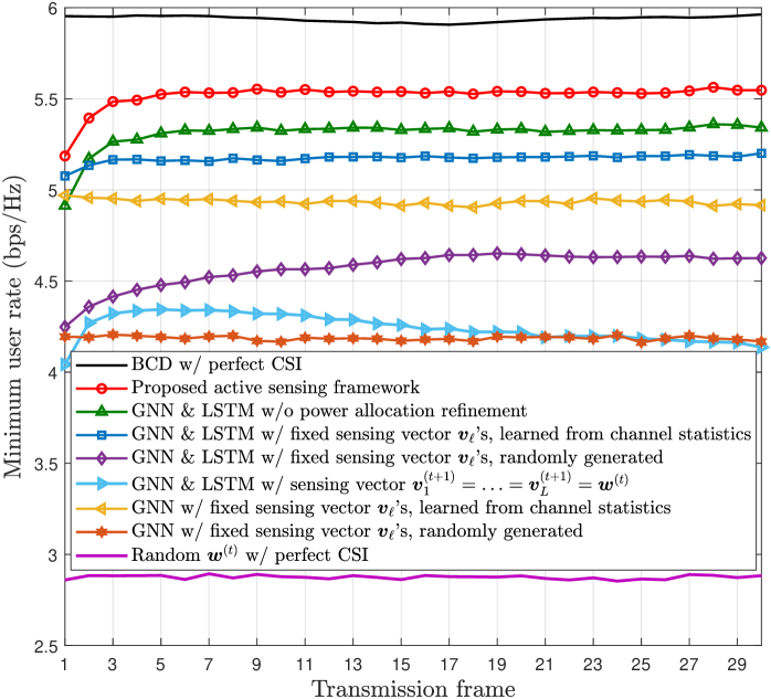
Figure 9: Average minimum user rate at the $1$-st block of each frame (i.e., $\min_{k}\{R_{k}^{(t,1)}\}$) for different beam tracking methods. Here, $L=3$, $M=8$, $N_{r}=100$, $K=3$, $N_{G}=8$, $\tau_{w}=10$.

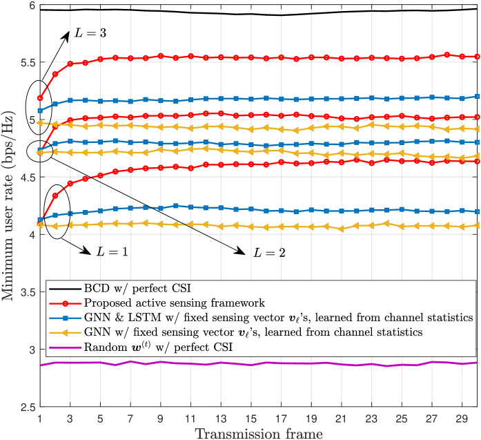
Figure 10: The impact of different number of sensing vectors $L$’s within each frame on different beam tracking methods. Here, $M=8$, $N_{r}=100$, $K=3$, $N_{G}=8$, $\tau_{w}=10$.

V-D Performance Comparison

Fig. 9 shows the downlink minimum user rate of different beam tracking methods in different transmission frames. The proposed active sensing framework initially achieves around $84\%$ of the BCD algorithm with perfect CSI, indicating efficient initial design based on the statistics of the UE mobility pattern. As the AP receives more pilots, the performance of the proposed approach improves quickly to $94\%$ of the performance of the benchmark with perfect CSI. This indicates that the proposed active sensing framework can efficiently exploit the temporal correlations of the time varying channel. Specifically, the beam tracking methods using both GNN and LSTM significantly outperform those benchmarks with only GNNs. This is because the LSTM-based methods are able to exploit the historical channel information to design the AP beamforming vectors and the downlink RIS reflection coefficients, thereby improving beam tracking performance over time. Among the beam tracking approaches with LSTM, the proposed framework performs the best, because it designs the RIS sensing vectors in an active manner. This shows the benefits of adaptively designing the RIS sensing vectors based on previously received pilots.

For the benchmarks with fixed sensing schemes, Fig. 9 shows that the ones with learned sensing vectors outperform those with random sensing vectors. This shows the performance gain of designing the RIS sensing vectors based on channel statistics. Additionally, the GNN & LSTM benchmark, which uses the same RIS reflection coefficients for both pilot acquisition and data transmission stages, performs less effectively as compared to other GNN & LSTM benchmarks that employ distinct RIS reflection coefficients for these two stages. This shows the importance of designing the RIS reflection coefficients in channel sensing and data transmission stages separately. Moreover, we remark that a $5\%$ performance improvement can be obtained from power allocation refinement.

Furthermore, Fig. 9 shows that the proposed framework maintains its performance for transmission frames beyond $20$, despite being trained with only $20$ concatenated active sensing units corresponding to $20$ frames. We also observe empirically that the proposed framework continues to sustain its performance over hundreds of frames by reusing the active sensing unit. This robust performance beyond the training range is due to the ability of the LSTM cells to effectively capture the UE mobility patterns and to consistently update channel information based on the latest received pilots.

Impact of Different $L$’s

Next, we evaluate the performance of the proposed approach for different number of sensing vector $L$’s within each frame. As can be seen from Fig. 10, the proposed active sensing framework always outperforms the benchmarks with fixed sensing strategies, because it leverages past observations to actively design the RIS sensing vectors. Furthermore, it is observed that LSTM-based methods (including the proposed approach) show faster convergence as the number of sensing sub-blocks $L$ increases. This is because a larger $L$ provides the LSTM with more observations in every frame, thereby facilitating more efficient capturing of temporal channel correlations.

V-E Interpretation of the Learned Solutions

In this section, we use the array response of the RIS and the SINR map as a means to illustrate qualitatively and quantitatively the correctness of the solutions learned by the proposed framework, respectively. In the pilot stage (i.e., $0$-th block) of the $t$-th frame, the array response of the RIS sensing vector $\bm{v}_{\ell}^{(t)}$ at the coordinates $[x,y]$ is given as [24]:

$$r_{\text{RIS}}(\phi_{2,1},\dots,\phi_{2,N_{G}},\theta_{3,[x,y]}^{(t,0)},\phi_{3,[x,y]}^{(t,0)},\bm{v}_{\ell}^{(t)})$$ (25)

$$=|(\sum_{i=1}^{N_{G}}\bm{a}_{\text{RIS}}(\theta_{2,i},\phi_{2,i}))^{\sf{H}}\operatorname{diag}(\bm{v}_{\ell}^{(t)})\bm{a}_{\text{RIS}}(\theta_{3,[x,y]}^{(t,0)},\phi_{3,[x,y]}^{(t,0)})|\ ,$$

where $\ell=1,\dots,L$ and $\theta_{2,i}=0$, $i=1,\dots,N_{G}$. Here, $\theta_{3,[x,y]}^{(t,n)}$ and $\phi_{3,[x,y]}^{(t,n)}$ denotes the elevation and azimuth AoA from the coordinates $[x,y]$ to the RIS. When the coordinates $[x,y]$ coincide with the actual location of the mobile UE $k$, $\theta_{3,[x,y]}^{(t,n)}$ and $\phi_{3,[x,y]}^{(t,n)}$ equivalents to $\theta_{3,k}^{(t,n)}$ and $\phi_{3,k}^{(t,n)}$ as in (23). Similarly, the array response of the downlink RIS reflection coefficients $\bm{w}^{(t)}$ in the $n$-th block of the $t$-th frame can be computed as $r_{\text{RIS}}(\phi_{2,1},\dots,\phi_{2,N_{G}},\theta_{3,[x,y]}^{(t,n)},\phi_{3,[x,y]}^{(t,n)},\bm{w}^{(t)})$. In addition, the array response of the downlink beamforming vector $\bm{b}_{k}^{(t)}$ can be expressed as:

$$r_{\text{AP},k}(\phi,\bm{b}_{k}^{(t)})=|\bm{a}_{\text{AP}}(\phi)^{\sf{H}}\bm{b}_{k}^{(t)}|\ ,k=1,\dots,K\ ,$$ (26)

where $\phi\sim\mathcal{U}(0,2\pi)$ is the effective AoA. We can further compute the SINR using the downlink beamformers $\{\bm{b}^{(t)}_{k}\}_{k=1}^{K}$ and RIS reflection coefficients $\bm{w}^{(t)}$ as follows:

$$\frac{|(\bm{A}^{(t,n)}_{[x,y]}\widetilde{\bm{w}}^{(t)})^{\sf{H}}\bm{b}_{k}^{(t)}|^{2}}{\sum_{j=1,j\neq k}^{K}|(\bm{A}^{(t,n)}_{[x,y]}\widetilde{\bm{w}}^{(t)})^{\sf{H}}\bm{b}_{j}^{(t)}|^{2}+\sigma_{d}^{2}}\ ,\ k=1,\dots,K\ ,$$ (27)

where $\bm{A}^{(t,n)}_{[x,y]}$ is the combined channel between the AP and the coordinates $[x,y]$ in the $n$-th block of the $t$-th frame. When the coordinates $[x,y]$ coincide with the actual location of the mobile UE $k$, the combined channel $\bm{A}^{(t,n)}_{[x,y]}$ equivalents to $\bm{A}^{(t,n)}_{k}$ as in (1).

Interpretation of the Downlink Beam Alignment Strategy

In Fig. 11(a), the array response of the downlink RIS reflection coefficients $\bm{w}^{(t)}$ shows that the proposed framework effectively tracks the UEs by progressively reflecting increasingly focused downlink beams via the RIS towards the actual positions of the mobile UEs. It is observed that the peaks corresponding to the first two UEs are sometimes weaker than the third UE, but we can see from Fig. 11(b) that these weaker UEs are compensated by stronger array response of the beamformers at the AP. Therefore, the proposed framework indeed learns to jointly optimize the downlink RIS reflection coefficients and the beamforming matrix to ensure fairness in maximizing the minimum rate across the three mobile UEs, while exploiting channel correlations to design improved RIS reflection coefficients and beamformers over time.

Interpretation of the Learned Solutions via SINR Map

we further plot the downlink SINR map for each mobile UE to show the overall beam tracking effectiveness of the proposed framework. As shown in Fig. 12, the SINR map broadly covers areas around the UEs initially, but progressively narrows to focus on actual positions of all three mobile UEs. This progressive focusing indicates that proposed framework is able to design sensible downlink beamformers $\bm{b}_{k}^{(t)}$ and data transmission RIS reflection coefficients $\bm{w}^{(t)}$ by utilizing both temporal and spatial information from the received pilots.

Interpretation of the Proposed Active Sensing Strategy

As illustrated in Fig. 13, the proposed framework designs $L=3$ RIS sensing vectors cooperatively. For example, in the pilot stage of the $30$-th frame, one UE (represented by the red dot) is not targeted by the first RIS sensing vector $\bm{v}_{1}^{(t)}$, but is focused by $\bm{v}_{2}^{(t)}$. Meanwhile, the weaker array response of $\bm{v}_{2}^{(t)}$ towards the green UE and $\bm{v}_{3}^{(t)}$ towards the blue UE are compensated by stronger responses from the other two sensing vectors, respectively. This cooperative sensing strategy is not seen in the initial tracking frame, but is progressively developed over time by leveraging historical channel observations. As a result, the proposed framework actively narrows the sensing range and enhances the pilot SNR in the uplink CSI acquisition stages, leading to more informative neural network inputs and improved beam tracking performance. In contrast, the GNN & LSTM benchmark employs a non-adaptive approach by using channel statistics to train fixed RIS sensing vectors, which cover nearly the entire service area for CSI acquisition. However, this broad coverage results in lower uplink SNR during CSI acquisition and, subsequently, higher pilot overhead.

VI Conclusion

This paper proposes an active sensing based beam tracking approach for RIS-assisted multiuser mobile communication systems. The proposed approach can adaptively design the AP beamformers and the RIS reflection coefficients for downlink data transmission, as well as the RIS reflection coefficients for uplink channel sensing. This is accomplished by utilizing an LSTM-based RNN to summarize received pilot information into state vectors, and a GNN to optimize the mapping from state vectors to the beam tracking matrices. Numerical results demonstrate that the proposed active sensing framework produces interpretable solutions and achieves significantly higher data rates than benchmark data-driven methods with non-adaptive sensing.

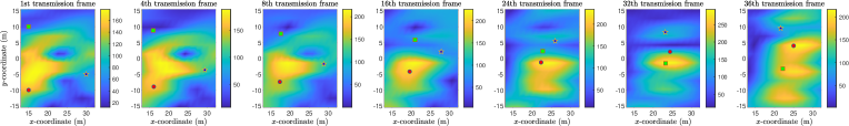
(a) Array response of the downlink RIS reflection coefficients $\bm{w}^{(t)}$ obtained by the proposed framework.

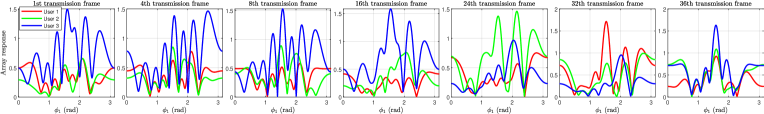
(b) Array response of the downlink beamforming vectors $\bm{b}^{(t)}_{k}$’s obtained by the proposed framework.

Figure 11: Array response of the downlink RIS reflection coefficients and beamformers obtained by the proposed framework in different frames. The proposed framework is tested on a randomly generated trajectory. Here, $L=3$, $M=8$, $N_{r}=100$, $K=3$, $N_{G}=8$, $\tau_{w}=10$.

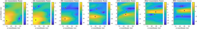
(a) SINR (dB) map of the UE $1$.

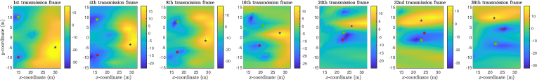
(b) SINR (dB) map of the UE $2$.

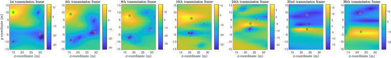
(c) SINR (dB) map of the UE $3$.

Figure 12: SINR (dB) map around the position of mobile UEs under the proposed active sensing framework in different frames. The proposed framework is tested on a randomly generated trajectory. Here, $L=3$, $M=8$, $N_{r}=100$, $K=3$, $N_{G}=8$, $\tau_{w}=10$.

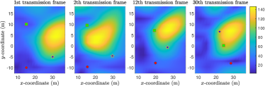
(a) $\bm{v}^{(t)}_{1}$, actively designed by the proposed framework.

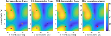
(b) Fixed $\bm{v}_{1}$, learned from channel statistics.

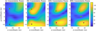
(c) $\bm{v}^{(t)}_{2}$, actively designed by the proposed framework.

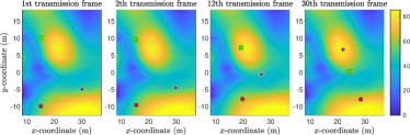
(d) Fixed $\bm{v}_{2}$, learned from channel statistics.

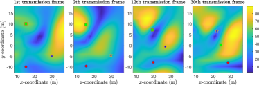
(e) $\bm{v}^{(t)}_{3}$, actively designed by the proposed framework.

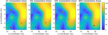
(f) Fixed $\bm{v}_{3}$, learned from channel statistics.

Figure 13: The array response of the RIS sensing vectors obtained by the proposed active sensing framework and by the GNN & LSTM benchmark without active sensing in the pilot stage (the 0-th block) across the different frames. Here, $L=3$, $M=8$, $N_{r}=100$, $K=3$, $N_{G}=8$, $\tau_{w}=10$.

References

- [1] H. Han, T. Jiang, and W. Yu, “Active beam tracking with reconfigurable intelligent surface,” in Proc. IEEE Int. Conf. Acoust., Speech Signal Process. (ICASSP), Rhodes Island, Greece, Jun. 2023, pp. 1–5.
- [2] M. Di Renzo, A. Zappone, M. Debbah, M.-S. Alouini, C. Yuen, J. de Rosny, and S. Tretyakov, “Smart radio environments empowered by reconfigurable intelligent surfaces: How it works, state of research, and the road ahead,” IEEE J. Sel. Areas Commun., vol. 38, no. 11, pp. 2450–2525, Jul. 2020.
- [3] Q.-U.-A. Nadeem, H. Alwazani, A. Kammoun, A. Chaaban, M. Debbah, and M.-S. Alouini, “Intelligent reflecting surface-assisted multi-user miso communication: Channel estimation and beamforming design,” IEEE Open J. Commun. Soc., vol. 1, pp. 661–680, 2020.
- [4] L. Wei, C. Huang, G. C. Alexandropoulos, C. Yuen, Z. Zhang, and M. Debbah, “Channel estimation for RIS-empowered multi-user MISO wireless communications,” IEEE Trans. Wireless Commun., vol. 69, no. 6, pp. 4144–4157, Jun. 2021.
- [5] Z. Wang, L. Liu, and S. Cui, “Channel estimation for intelligent reflecting surface assisted multiuser communications: Framework, algorithms, and analysis,” IEEE Trans. Wirel. Commun., vol. 19, no. 10, pp. 6607–6620, 2020.
- [6] F. Sohrabi, T. Jiang, W. Cui, and W. Yu, “Active sensing for communications by learning,” IEEE J. Sel. Areas Commun., vol. 40, no. 6, pp. 1780–1794, Jun. 2022.
- [7] S. Hochreiter and J. Schmidhuber, “Long short-term memory,” Neural Comput., vol. 9, no. 8, pp. 1735–1780, Nov. 1997.
- [8] W. Hamilton, Z. Ying, and J. Leskovec, “Inductive representation learning on large graphs,” Adv. Neural Inf. Process. Syst., vol. 30, 2017.
- [9] S. E. Zegrar, L. Afeef, and H. Arslan, “A general framework for ris-aided mmwave communication networks: Channel estimation and mobile user tracking,” Sept. 2020. [Online]. Available: https://arxiv.org/abs/2009.01180
- [10] D. Yu, G. Zheng, A. Shojaeifard, S. Lambotharan, and Y. Liu, “Kalman filter based channel tracking for RIS-assisted multi-user networks,” IEEE Trans. Wireless Commun., pp. 1–1, 2023.
- [11] T. Li, H. Tong, Y. Xu, X. Su, and G. Qiao, “Double IRSs aided massive MIMO channel estimation and spectrum efficiency maximization for high-speed railway communications,” IEEE Trans. Veh. Technol., vol. 71, no. 8, pp. 8630–8645, 2022.
- [12] P. Cai, J. Zong, X. Luo, Y. Zhou, S. Chen, and H. Qian, “Downlink channel tracking for intelligent reflecting surface-aided FDD MIMO systems,” IEEE Trans. Veh. Technol., vol. 70, no. 4, pp. 3341–3353, Apr. 2021.
- [13] Y. Wei, M.-M. Zhao, A. Liu, and M.-J. Zhao, “Channel tracking and prediction for IRS-aided wireless communications,” IEEE Trans. Wireless Commun., vol. 22, no. 1, pp. 563–579, 2023.
- [14] V. Va, H. Vikalo, and R. W. Heath, “Beam tracking for mobile millimeter wave communication systems,” in Proc. IEEE Glob. Conf. Signal Inf. Process. (GlobalSIP), 2016, pp. 743–747.
- [15] K. Guo, M. Wu, X. Li, H. Song, and N. Kumar, “Deep reinforcement learning and NOMA-based multi-objective RIS-assisted IS-UAV-TNs: Trajectory optimization and beamforming design,” IEEE Trans. Intell. Transp. Syst., vol. 24, no. 9, pp. 10 197–10 210, 2023.
- [16] L. Wang, K. Wang, C. Pan, and N. Aslam, “Joint trajectory and passive beamforming design for intelligent reflecting surface-aided UAV communications: A deep reinforcement learning approach,” IEEE Trans. Mob. Comput., vol. 22, no. 11, pp. 6543–6553, 2023.
- [17] J. Yu, X. Liu, Y. Gao, C. Zhang, and W. Zhang, “Deep learning for channel tracking in IRS-assisted UAV communication systems,” IEEE Trans. Wireless Commun., vol. 21, no. 9, pp. 7711–7722, 2022.
- [18] C. Liu, X. Liu, Z. Wei, D. W. K. Ng, and R. Schober, “Scalable predictive beamforming for IRS-assisted multi-user communications: A deep learning approach,” Nov. 2022. [Online]. Available: https://arxiv.org/abs/2211.12644
- [19] G. Dulac-Arnold, N. Levine, D. J. Mankowitz, J. Li, C. Paduraru, S. Gowal, and T. Hester, “Challenges of real-world reinforcement learning: definitions, benchmarks and analysis,” Mach. Learn., vol. 110, no. 9, pp. 2419–2468, 2021.
- [20] M. Eisen and A. Ribeiro, “Optimal wireless resource allocation with random edge graph neural networks,” IEEE Trans. Signal Process., vol. 68, pp. 2977–2991, 2020.
- [21] M. Lee, G. Yu, and G. Y. Li, “Graph embedding-based wireless link scheduling with few training samples,” IEEE Trans. Wirel. Commun., vol. 20, no. 4, pp. 2282–2294, 2021.
- [22] Y. Shen, Y. Shi, J. Zhang, and K. B. Letaief, “Graph neural networks for scalable radio resource management: Architecture design and theoretical analysis,” IEEE J. Sel. Areas Commun., vol. 39, no. 1, pp. 101–115, 2021.
- [23] J. Kim, H. Lee, S.-E. Hong, and S.-H. Park, “A bipartite graph neural network approach for scalable beamforming optimization,” IEEE Trans. Wirel. Commun., vol. 22, no. 1, pp. 333–347, 2023.
- [24] T. Jiang, H. V. Cheng, and W. Yu, “Learning to reflect and to beamform for intelligent reflecting surface with implicit channel estimation,” IEEE J. Sel. Areas Commun., vol. 39, no. 7, pp. 1931–1945, Jul. 2021.
- [25] T. L. Jensen and E. De Carvalho, “An optimal channel estimation scheme for intelligent reflecting surfaces based on a minimum variance unbiased estimator,” in Proc. IEEE Int. Conf. Acoust., Speech Signal Process. (ICASSP), May 2020, pp. 5000–5004.
- [26] Z. Zhang, T. Jiang, and W. Yu, “Localization with reconfigurable intelligent surface: An active sensing approach,” IEEE Trans. Wirel. Commun., pp. 1–1, 2023.
- [27] S.-E. Chiu, N. Ronquillo, and T. Javidi, “Active learning and csi acquisition for mmWave initial alignment,” IEEE J. Sel. Areas Commun., vol. 37, no. 11, pp. 2474–2489, 2019.
- [28] F. Sohrabi, Z. Chen, and W. Yu, “Deep active learning approach to adaptive beamforming for mmWave initial alignment,” IEEE J. Sel. Areas Commun., vol. 39, no. 8, pp. 2347–2360, Aug. 2021.
- [29] T. Jiang, F. Sohrabi, and W. Yu, “Active sensing for two-sided beam alignment and reflection design using ping-pong pilots,” IEEE J. Sel. Areas Inf. Theory., vol. 4, pp. 24–39, 2023.
- [30] T. Jiang and W. Yu, “Active sensing for reciprocal MIMO channels,” in Proc. IEEE 23rd Int. Workshop Signal Process. Adv. Wireless Commun. (SPAWC), 2023, pp. 166–170.
- [31] Z. Zhang, T. Jiang, and W. Yu, “Learning based user scheduling in reconfigurable intelligent surface assisted multiuser downlink,” IEEE J. Sel. Top. Signal Process., vol. 16, no. 5, pp. 1026–1039, 2022.
- [32] J. Chen, Y.-C. Liang, H. V. Cheng, and W. Yu, “Channel estimation for reconfigurable intelligent surface aided multi-user mmwave MIMO systems,” IEEE Trans. Wireless Commun., pp. 1–1, 2023.
- [33] W. Yu, F. Sohrabi, and T. Jiang, “Role of deep learning in wireless communications,” IEEE BITS Info. Th. Magazine, pp. 1–14, 2022.
- [34] E. Björnson, M. Bengtsson, and B. Ottersten, “Optimal multiuser transmit beamforming: A difficult problem with a simple solution structure [lecture notes],” IEEE Signal Process. Mag., vol. 31, no. 4, pp. 142–148, 2014.
- [35] S. Liang and R. Srikant, “Why deep neural networks for function approximation?” in Proc. Int. Conf. Learn. Represent. (ICLR), 2017.
- [36] S. Ravanbakhsh, J. Schneider, and B. Poczos, “Equivariance through parameter-sharing,” in Proc. Int. Conf. Mach. Learn. (ICML). PMLR, 2017, pp. 2892–2901.
- [37] D. P. Kingma and J. Ba, “Adam: A method for stochastic optimization,” Dec. 2014. [Online]. Available: https://arxiv.org/abs/1412.6980
- [38] Q.-U.-A. Nadeem, A. Kammoun, A. Chaaban, M. Debbah, and M.-S. Alouini, “Asymptotic max-min SINR analysis of reconfigurable intelligent surface assisted MISO systems,” IEEE Trans. Wirel. Commun., vol. 19, no. 12, pp. 7748–7764, 2020.
- [39] D. W. H. Cai, T. Q. S. Quek, and C. W. Tan, “A unified analysis of max-min weighted sinr for MIMO downlink system,” IEEE Trans. Signal Process., vol. 59, no. 8, pp. 3850–3862, 2011.
- [40] M. Abadi et al., “Tensorflow: Large-scale machine learning on heterogeneous distributed systems,” Mar. 2016. [Online]. Available: https://arxiv.org/abs/1603.04467
- [41] X. Yu, D. Xu, and R. Schober, “MISO wireless communication systems via intelligent reflecting surfaces,” in 2019 IEEE/CIC Int. Conf. Commun. China (ICCC). IEEE, 2019, pp. 735–740.
- [42] T. Jiang and W. Yu, “Interference nulling using reconfigurable intelligent surface,” IEEE J. Sel. Areas Commun., vol. 40, no. 5, pp. 1392–1406, 2022.