Learning from Students: Applying t-Distributions
to Explore Accurate and Efficient Formats for LLMs

Abstract

Large language models (LLMs) have recently achieved state-of-the-art performance across various tasks, yet due to their large computational requirements, they struggle with strict latency and power demands. Deep neural network (DNN) quantization has traditionally addressed these limitations by converting models to low-precision integer formats. Yet recently alternative formats, such as Normal Float (NF4), have been shown to consistently increase model accuracy, albeit at the cost of increased chip area. In this work, we first conduct a large-scale analysis of LLM weights and activations across 30 networks to conclude most distributions follow a Student’s t-distribution. We then derive a new theoretically optimal format, Student Float (SF4), with respect to this distribution, that improves over NF4 across modern LLMs, for example increasing the average accuracy on LLaMA2-7B by 0.76% across tasks. Using this format as a high-accuracy reference, we then propose augmenting E2M1 with two variants of supernormal support for higher model accuracy. Finally, we explore the quality and performance frontier across 11 datatypes, including non-traditional formats like Additive-Powers-of-Two (APoT), by evaluating their model accuracy and hardware complexity. We discover a Pareto curve composed of INT4, E2M1, and E2M1 with supernormal support, which offers a continuous tradeoff between model accuracy and chip area. For example, E2M1 with supernormal support increases the accuracy of Phi-2 by up to 2.19% with 1.22% area overhead, enabling more LLM-based applications to be run at four bits.

1. Cornell University  2. Google

1 Introduction

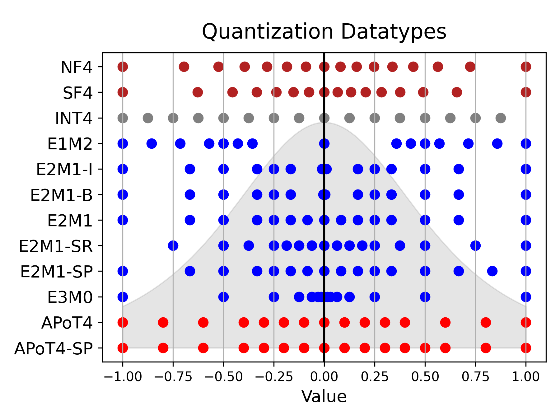
Figure 1: Quantization Datatypes – Datatypes should reflect DNN weight and activation distributions to achieve the highest quality. In this work, we compare model accuracy, chip area, and power consumption across datatypes to map the quality-efficiency Pareto frontier. We also propose alternative datatypes including Student Float (SF4), super-range E2M1 (SR), and super-precision E2M1 (SP). These complement existing Normal Float (NF4), Intel E2M1 (E2M1-I), bitsandbytes E2M1 (E2M1-B) and Additive Powers of Two (APoT4) datatypes.

Quantization has become the mainstream method for deep neural network (DNN) compression (Hao et al., 2021). Compared to alternatives like pruning, it retains original model quality at higher compression ratios (Kuzmin et al., 2023), and importantly it can be applied post-training, often without any fine-tuning. This makes it suitable for large language models (LLMs), which require significant resources during fine-tuning for gradient and optimizer state buffers. Recent LLM quantization works have successfully lowered weight and activation precision to eight bits (Frantar et al., 2023; Xiao et al., 2023) and four bits (Zhao et al., 2023; Liu et al., 2023; Shao et al., 2023) with minimal accuracy loss.

At four bits, prior LLM quantization has focused on integer datatypes since they are supported in current DNN accelerators (Jouppi et al., 2023). However, recent work has shown eight-bit floating-point (FP8), e.g. E4M3, achieves higher accuracy compared to INT8, where E represents the number of exponent bits and M the number of mantissa bits (Kuzmin et al., 2022; Micikevicius et al., 2022; Shen et al., 2023). These improvements motivate the further study of four-bit non-integer formats, such as FP4, which can be included in next-generation DNN accelerators.

Figure 1 shows seven FP4 variants in blue, along with INT4 and multiple alternative formats. These formats are all normalized to one for comparison and set against an example weight or activation distribution in the background. The agreement between the datatype shape and the distributions being quantized primarily determines the model accuracy. For example, typically E2M1 achieves higher accuracy than INT4 because it allocates more coverage to the center of data distribution where the majority of values are found. This is particularly important at four bits, since at higher bitwidths, there are enough values that most datatypes can provide dense coverage, reducing the differences among datatypes.

In addition to model quality, datatypes must also have efficient multiply-and-accumulate (MAC) units, which perform nearly all of the compute-intensive LLM operations. For instance, while E2M1 has higher accuracy, up to a 7.13% LAMBADA improvement on Phi-2, INT4 has an 8% smaller and more power-efficient MAC unit. In this work, we explore this accuracy-efficiency frontier and summarize our contributions as follows:

1. Conduct a large-scale profiling of the weights and activations across 30 DNNs and discover that most DNN distributions are best approximated by the Student’s t-distribution.

2. Derive a theoretically optimal datatype with respect to this distribution, Student Float (SF4), and empirically verify that it improves the state-of-the-art for lookup-based weight-only quantization.

3. Propose two variants of supernormal support for E2M1 and Additive Powers-of-Two (APoT) datatypes, using SF4 as a high-accuracy reference.

4. Plot the Pareto frontier for accuracy and performance across datatypes, comparing FP4 vs. INT4, discussing FP4 variants, and improving the accuracy of E2M1 and APoT4 with supernormal support.

2 Related Work

DNN quantization can be broadly categorized into two branches: quantization-aware training (QAT) (Zhang et al., 2023a) and post-training quantization (PTQ) (Zhao et al., 2019). PTQ directly performs quantization after the model has finished training, often without any training or calibration data (Cai et al., 2020; Nagel et al., 2019). This data-free approach simplifies the model deployment process and reduces compute, but this simplicity typically leads to lower model accuracy, especially at low precision. In this scenario, the choice of datatype is particularly important in preserving high model accuracy. Traditionally, integer was the only option at low precision, yet recent work has proposed floating-point, lookup-based datatypes, and more complex alternative formats. At four bits, these datatypes have complex quality and performance trade-offs that affect the model accuracy, chip area, and estimated power.

2.1 Floating-Point

Floating-point formats like FP32, FP16, and BF16 have been essential for deep learning given their ability to represent a wide range of values necessary for weights, activations, and gradients. Recently, the Open Compute Project proposed a standard for lower-precision formats, including FP4, FP6, and micro-scaling formats (Rouhani, 2023), which share exponents and scale factors at the block level. This standard follows prior research like VS-Quant (Dai et al., 2021) and micro-exponents (MX) (Rouhani et al., 2023), which share scales per block and introduce multi-level scale factors. In addition, the quantization library “bitsandbytes” (Dettmers et al., 2022a) has implemented an FP4 datatype for weight-only LLM quantization. This library provides the primary quantization support for Hugging Face transformers, which is the most popular framework for LLMs (Wolf et al., 2020). Similarly, Intel’s neural compressor, which has become a popular library for LLM compression research, offers an FP4 implementation for weight-only LLM quantization (Shen et al., 2023).

In addition to new standards and tools, multiple recent works have compared floating-point against integer formats. FLIQS (Dotzel et al., 2024) and MoFQ (Zhang et al., 2023b) discovered that floating-point formats produce higher accuracies across vision, language, and recommendation tasks, where the differences are larger at lower precisions. Our work continues this line of research by comparing seven different FP4 candidates across LLMs, proposing supernormal extensions to them, and mapping their quality and hardware efficiency tradeoffs.

2.2 Logarithmic Datatypes

Floating-point formats become logarithmic formats when all bits are allocated to the exponent. These formats have been considered for accelerating DNNs since they replace the costly digital multiplications (Alsuhli et al., 2023) with exponent addition. Early works used logarithmic numbers to accelerate convolutional neural networks (CNNs) (Miyashita et al., 2016), yet they often led to lower model accuracy, since their datatype shape does not match the natural DNN distributions, as shown in Figure 1.

Additive Powers-of-Two (APoT) addresses this quality issue by adding two logarithmic numbers to better fit DNN distributions (Li et al., 2020) and increase model accuracy. At four bits, the APoT4 format has the form: $(-1)^{S}\,(2^{E}+2^{\tilde{E}})$, where $E\in\{0,2^{-1},2^{-2},2^{-4}\}$ and $\tilde{E}\in\{0,2^{-3}\}$. Our work maps the quality-efficiency frontier of these formats, describes the limitations of native E3M0, and introduces two variants of E3M0 and APoT that achieve higher accuracy with minor area overhead.

2.3 Normal Float

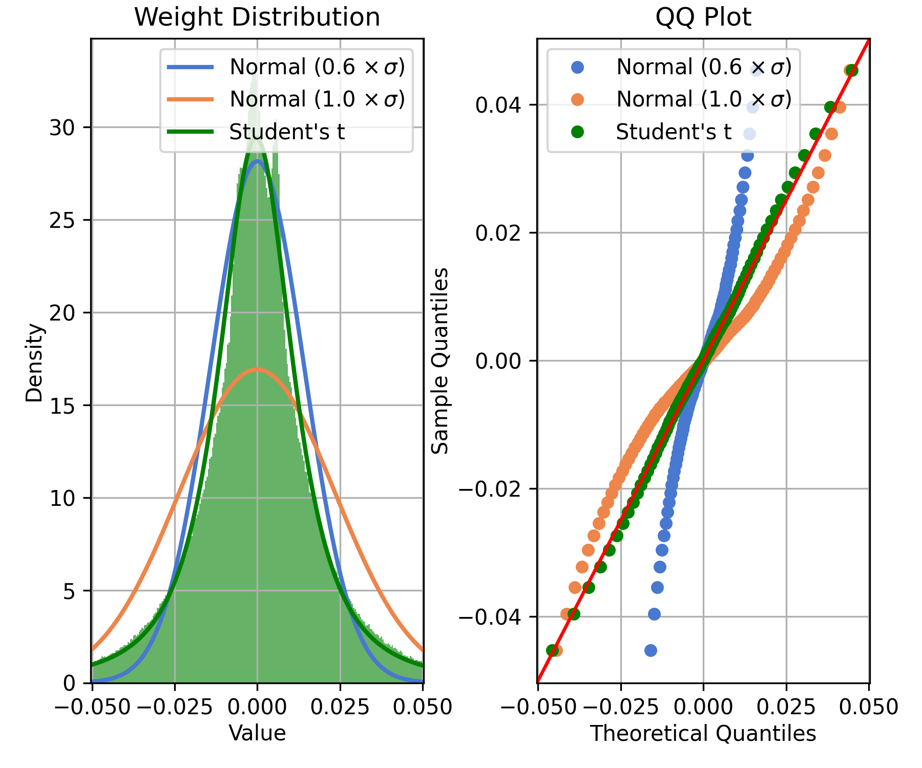
Figure 2: Mistral-7B Weight Profile – The weights in Mistral-7B are best approximated by t-distributions. The best fitting normal distribution (1.0 $\times$ $\sigma$) poorly fits the peak of the distribution, and forcing it to fit the peak (0.6 $\times$ $\sigma$) causes poor representation on the larger values. Straight lines on quantile-quantile (Q-Q) plots indicate perfect fits between theoretical and sampled distributions.

While logarithmic datatypes were developed primarily for performance, Normal Float (NF4) was constructed for model accuracy (Dettmers et al., 2023). It equally divides the probability mass for normal distributions using quantile functions (Dettmers et al., 2022b), ensuring approximately the same number of weights get mapped to each datatype value. This leads to high accuracy, yet it relies on floating-point lookup tables and high-precision MAC units to be implemented in real hardware. In our work, we propose an alternate lookup format, Student Float (SF4), to increase the accuracy of weight-only quantized LLMs and build various hardware-efficient datatypes based on its insights.

2.4 Distribution Profiling

Multiple DNN compression works have performed small-scale studies on weights and activations to motivate their work. For example, QLoRA (Dettmers et al., 2023) used the Shapiro-Wilk normality test on LLaMA2-7B weights to argue that many weights are approximately normally distributed while developing NF4. A few earlier works, however, noticed DNN weights often deviate from normal distributions (Guo et al., 2022). ACIQ (Banner et al., 2018) classified many weights as Laplace distributions, which is a more peaked and centralized distribution, and later OCS (Zhao et al., 2019) found that squared Laplace distributions provided the best fit. We expand on this profiling work by studying the weight and activation distributions from over 30 DNNs, including popular LLMs such as LLaMA2, Phi-2, and Mistral-7B.

3 Proposed Datatypes

Model	Weight		Activation
	$\nu$	KS-$\Delta$	$\nu$	KS-$\Delta$
OPT-1B	6.682.86	0.040	5.914.08	0.117
BLOOM-560M	5.872.68	0.020	6.754.84	0.066
BLOOM-7B	10.135.96	-0.019	4.511.33	0.049
Falcon-7B	5.872.68	0.020	6.754.84	0.066
LLaMA2-7B	6.783.45	0.025	2.980.89	0.022
Yi-6B	7.264.98	0.013	2.503.30	0.036
FLAN-T5	13.472.40	0.004	5.341.53	0.031
Mistral-7B	1.660.67	0.049	1.672.15	0.111
Zephyr-3B	4.595.20	0.099	2.371.03	0.098
BERT	13.132.42	-0.069	6.454.35	0.034
RoBERTa	7.282.18	0.022	6.694.77	0.022
ALBERT	10.874.86	0.000	7.811.75	0.018
ResNet18	2.710.69	0.069	10.946.20	-0.008
ResNet50	2.951.22	0.052	6.577.03	0.006
MobileNetV2	5.025.55	0.003	8.227.92	0.003
EfficientNet-B0	4.295.42	0.065	3.511.86	0.029

Table 1: Weight and Activation Profiling – DNN distributions are better approximated by t-distributions, typically with single-digit degrees of freedom ($\nu$). The mean and variance for $\nu$ are calculated across layers. The Kolmogorov-Smirnov (KS) $\Delta$ measures the difference between the KS distance run on the best-fit normal and Student’s t-distributions. Positive values indicate a smaller distance to the t-distribution.

In this section, we conduct a large-scale profiling of LLM weight and activation distributions across models and applications. We then use these distributions to analytically derive the SF4 datatype and introduce supernormal support, which increases model accuracy for E2M1 and APoT4 formats with low hardware overhead.

3.1 Student’s t-Distribution

Instead of the normal distribution, we use the Student’s t-distribution to model LLM weights and activations. This distribution, $S(t;\mu,\tau^{2},\nu)$, generalizes the normal distribution by introducing a degree of freedom parameter $\nu$ that controls its peaks and tails. Larger $\nu$ leads to wider peaks and thinner tails, and vice versa (shown in Appendix E). In addition, the $\mu$ offset parameter allows it to model distributions with non-zero means, and $\tau^{2}$ controls its overall scale. In context, the offset $\mu$ is important for matching activation distributions, which are often skewed due to asymmetric activation functions. The t-distribution probability density function (PDF) is shown below for $\mu=0$ and $\tau^{2}=1$, where $\Gamma$ is the generalized factorial.

$$S(t) =\frac{\Gamma\left(\frac{\nu+1}{2}\right)}{\sqrt{\nu\pi}\,\Gamma\left(\frac{\nu}{2}\right)}\left(1+\frac{t^{2}}{\nu}\right)^{-\frac{\nu+1}{2}}$$ (1)

As $\nu\to\infty$, this distribution converges to the standard normal distribution. This is useful for studying LLM weights and activations, since if the distributions are normal, then $\nu$ will be relatively high during profiling. Likewise, as $\nu\to 1$, it approaches the Cauchy distribution, which has thinner peaks and fatter tails. The PDFs for these two cases are shown below:

$$S(t;\nu\to\infty) =\frac{1}{\sqrt{2\pi}}e^{-\frac{t^{2}}{2}}$$ (2)

$$S(t;\nu\to 1) =\frac{1}{\pi}\left(1+t^{2}\right)^{-1}$$ (3)

Figure 2 (left) shows the histogram of an MLP weight tensor from Mistral-7B (Jiang et al., 2023) along with the t-distribution and standard normal distribution. It demonstrates the best-fit t-distribution gives a better representation compared to the best-fit normal distribution ($1.0\times\sigma$) at small and large values. Furthermore, it shows that this is not just a matter of incorrect scaling. Since when $\sigma$ is scaled down by 0.6 in the normal distribution to fit the peak, the larger values are no longer well-represented. The right figure shows the same results in a quantile-quantile (Q-Q) plot, which compares the theoretical quantiles of each distribution to the profiled quantiles of the weight tensor. In a Q-Q plot, straight lines represent perfect matches, and therefore the t-distribution represents a much stronger fit overall.

Algorithm 1 Student Float Derivation

1:  Set $\delta=\frac{1}{2}\left(\frac{1}{32}+\frac{1}{30}\right)$.

2:  Compute eight evenly spaced probabilities $p_{1},\ldots,p_{8}$ where $p_{1}=\delta$ and $p_{8}=\frac{1}{2}$, and then compute eight evenly spaced probability values $p_{8},\ldots,p_{16}$ such that $p_{8}=\frac{1}{2}$ and $p_{16}=1-\delta$.

3:  Set $\tilde{s}_{i}=Q_{S}(p_{i};\nu)$ where $Q_{S}$ is the quantile function for the Student’s t-distribution $S(t;\nu$) with degrees of freedom $\nu$.

4:  Normalize $\tilde{s}$ to $[-1,1]$: $s_{i}=\frac{\tilde{s}_{i}}{\max_{i}|\tilde{s}_{i}|}$.

Table 1 expands this analysis by quantifying the mean and variance for $\nu$ across layers in LLMs, BERT-like models, and CNNs. It shows that the best fitting t-distributions typically have small single-digit degrees of freedom ($\nu$), with a few exceptions like the weights in FLAN-T5 (Wei et al., 2022) and BERT (Devlin et al., 2019). This implies they are significantly different from normal distributions on average. The table also quantifies the distribution fit by listing the difference between the Kolmogorov-Smirnov (KS) distances for the best-fitting t-distribution and normal distributions. The positive differences in most models indicate that the t-distribution has an overall better fit. More networks and analysis are in Appendix A.

3.2 Student Float

		OPT-125M		OPT-1B		Phi-2		LLaMA2-7B
	$\nu$	PPL	ACC	PPL	ACC	PPL	ACC	PPL	ACC
FP32	-	26.02	37.90	6.64	57.89	5.52	62.57	3.40	73.92
NF4	-	33.77	34.06	7.21	56.43	6.47	60.94	3.71	71.98
SF4	3	29.24	37.18	7.65	54.92	6.38	61.07	3.58	72.38
SF4	4	27.21	37.30	6.95	57.50	6.26	61.19	3.52	72.54
SF4	5	25.69	38.56	6.90	57.83	6.33	61.56	3.60	72.42
SF4	6	25.80	37.90	6.70	58.59	6.34	60.92	3.69	71.82
SF4	7	29.22	36.43	6.81	58.08	6.48	60.33	3.69	71.80

Table 2: Degrees of Freedom – LLM evaluation on LAMBADA accuracy (ACC) and perplexity (PPL). SF4 achieves its highest quality when generated with the most common degrees of freedom ($\nu$) profiled in Table 1. SF4 converges to NF4 in the limit (shown in Appendix E), yet its accuracy peaks around $\nu=5$.

		Mistral-7B		OPT-1B		OPT-6.7B		LLaMA2-7B		Phi-2		BLOOM-7B		Yi-6B
Calib. Method		None	MSE	None	MSE	None	MSE	None	MSE	None	MSE	None	MSE	None	MSE
LAMBADA ↑	FP32	75.90	75.90	57.89	57.89	67.69	67.69	73.92	73.92	62.57	62.57	57.64	57.64	68.27	68.27
	NF4	74.97	74.97	56.43	56.37	67.88	68.43	71.20	71.98	61.28	60.94	57.03	57.09	67.46	68.19
	SF4	75.90	75.00	58.02	57.83	68.02	68.02	71.96	72.42	60.47	61.56	57.97	57.87	67.84	68.04
	INT4	73.92	73.74	55.52	56.96	63.92	67.07	72.06	70.19	58.59	55.11	56.08	56.14	64.93	61.75
	E2M1-I	74.17	74.36	56.18	56.53	67.49	66.02	71.43	70.72	58.20	59.15	55.75	55.82	64.39	62.12
	E2M1-B	73.98	73.65	55.73	57.13	66.97	65.55	70.75	70.68	58.32	59.91	55.64	55.72	63.92	60.64
	E2M1	74.75	74.81	56.26	57.52	67.84	67.86	72.40	71.51	59.95	58.92	56.51	56.48	66.74	66.95
	+ SR	72.95	72.95	54.41	54.41	67.26	67.26	71.07	71.07	62.24	62.24	50.18	50.34	59.97	60.01
	+ SP	75.41	74.99	55.85	57.46	67.24	67.36	71.65	71.84	61.73	60.97	56.86	56.72	67.38	67.45
	E3M0	74.23	71.05	52.36	53.02	62.64	64.47	69.92	68.66	54.96	55.58	56.47	56.42	65.15	65.38
	APoT4	75.41	73.78	56.22	54.67	66.08	67.53	72.77	71.58	59.62	59.97	57.02	57.12	68.19	68.07
	+ SP	75.12	74.05	55.27	55.25	65.92	68.06	73.22	71.63	61.09	61.50	57.13	57.23	68.04	68.31

Table 3: Weight-Only Eval – Student Float (SF4) typically outperforms NF4, and the super normal variants (SR and SP) often improve over E2M1 and APoT4 although there are many exceptions. All models evaluated with weight-only sub-channel quantization with block size 128 with optional MSE clipping calibration. Further evaluations on WikiText-2 are in Appendix B.

Given these results, we can a generate datatype that optimizes for these profiled t-distributions by optimizing some quantity that correlates with model accuracy. In this section, we choose to minimize the difference between the number of weights or activations mapped to each datatype value. This effectively equalizes the load across the datatype and ensures the quantized histogram for SF4 will be approximately flat. This process is described in Algorithm 4, which was adapted from the NF4 process (Dettmers et al., 2023). It first generates sixteen numbers, $p_{i}$, equally spread out in probability space, and then maps these through the quantile function, $Q(p)$. This quantile function gives the value $x=Q(p)$, such that $S(X\leq x)=p$, where $X$ is a random variable following the t-distribution $S$. Therefore, equally spread probabilities will be mapped to quantiles that equally divide the probability mass.

Table 2 shows a small study on choosing the degrees of freedom ($\nu$) for SF4 and measures the LAMBADA accuracy and perplexity on OPT-125M, OPT-1B, Phi-2, and LLaMA2-7B. It shows the highest accuracy and lowest perplexity results typically cluster around $\nu=5$, which is close to the most common $\nu$ profiled in Table 1. This supports the claim that optimizing for equal load across the datatype typically leads to the highest accuracy. Then, as $\nu$ increases, the peaks of the t-distribution become shorter and wider, SF4 spreads out more, and in the limit, it converges to NF4 (shown in Appendix E). This table shows that SF4 reaches its highest accuracy significantly before converging to NF4. In Section 4, we choose $\nu=5$ for all SF4 datatypes for simplicity and to provide a single drop-in replacement for NF4.

3.3 Supernormal Support

	LAMB	Hella	Wino	PIQA	BoolQ	ARC-c	$\Delta$%
FP32	73.92	57.14	69.14	78.07	77.74	43.43	0.00
NF4	72.35	56.55	69.53	76.99	77.40	42.49	-1.10
SF4	73.20	56.81	69.06	77.69	78.56	43.34	-0.22
INT4	72.06	56.53	69.14	77.31	76.76	42.92	-1.17
E2M1-I	71.43	56.50	68.90	77.80	77.06	42.66	-1.30
E2M1-B	70.75	56.54	68.98	77.58	76.73	43.34	-1.28
E2M1	71.65	56.69	69.53	77.97	78.13	42.49	-0.85
+ SR	71.07	54.66	66.85	76.77	73.55	42.41	-3.49
+ SP	71.65	56.84	69.43	77.99	78.26	42.49	-0.80
E3M0	69.92	54.61	67.64	76.55	75.32	39.59	-4.32
APoT4	72.77	56.27	68.27	78.07	77.55	43.17	-0.86
+ SP	73.22	56.56	68.59	77.69	77.68	43.86	-0.39

Table 4: LLaMA2-7B Weight-Only – Accuracy improvements with SF4 and super-precision formats continue common zero-shot benchmarks. $\Delta$% represents the mean relative percentage change in accuracy from FP32. All models shown in Appendix I.

Given its high accuracy, SF4 can be used as a reference for building efficient datatypes. Figure 1 includes five E2M1 variants in comparison to SF4 and shows the importance of correctly choosing the subnormal bias. E2M1-I and E2M1-B push their subnormal values too close to zero, which will introduce large quantization errors on the most numerous central values in the distribution.

Beyond subnormal support, E2M1 and SF4 use a different number of values, where E2M1 only uses 15 unique values and SF4 uses all $2^{4}=16$ values. This missing value is caused by the floating-point sign bit, which introduces positive and negative zeros. At higher precision, this redundancy does not affect FP8 since these waste only 0.4% of its bitspace, but it makes a large difference at four bits, where FP4 wastes 6.25% of its values. Therefore, we propose adding additional supernormal support to E2M1 to complement the existing subnormal support. This reassigns negative zero to a useful value and brings these formats more in line with the SF4 datatype shape. In the following sections, we evaluate the accuracy and efficiency of two supernormal variants:

1. Super-range (SR), which extends the range of the values by allocating one point at the edge of the distribution.

2. Super-precision (SP), which extends the precision by giving one extra value within the distribution.

Super-precision matches the symmetry of SF4 and often achieves higher accuracy compared to super-range, yet it leads to larger chip area and power. For instance, it decreases the WikiText-2 perplexity compared to super-range across LLMs, including LLaMA2-7B, OPT1B, and Phi-2, while increasing the area of the corresponding MAC unit by 14%. Finally, we also add super-precision support to the APoT4 (Li et al., 2020) datatype in an analogous way. All datatype values are listed explicitly in Appendix F.

4 Experiments

In this section, we evaluate these proposed datatypes in addition to previous integer, floating-point, logarithmic, and lookup datatypes. These datatypes are evaluated across models, metrics, and methods totaling over 4000 data points. The main results are shown in this section, and the remainder are located the Appendix.

4.1 Language Models

Block Size	16	32	64	128	256	CW
NF4	-1.19	-0.89	-1.79	-1.87	-1.44	-4.86
SF4	-1.04	-1.04	-1.38	-1.33	-1.44	-3.69
INT4	-1.98	-2.27	-2.27	-2.96	-3.53	-7.98
E2M1-I	-1.90	-1.70	-2.02	-2.67	-3.37	-6.57
E2M1-B	-2.33	-2.00	-2.17	-2.80	-3.90	-8.58
E2M1	-1.27	-1.59	-1.67	-1.40	-1.62	-3.92
+ SR	-13.54	-4.98	-1.91	-1.86	-1.58	-3.21
+ SP	-0.39	-0.97	-0.92	-0.66	-0.92	-3.85
E3M0	-3.25	-3.33	-4.20	-4.50	-5.77	-6.17
APoT4	-1.34	-2.04	-2.34	-1.90	-2.30	-4.35
+ SP	-0.64	-1.47	-1.13	-1.29	-1.64	-3.43

Table 5: Phi-2 Subchannel Sweep – Differences between formats exist even with the smallest subchannel block sizes. All results are from Phi-2 with weight-only quantization. The average relative accuracy change (↑) from FP32 is shown, calculated across LAMBADA, HellaSwag, Winogrande, PIQA, BoolQ and ARC-c. Channelwise (CW) quantization is shown in the last column.

		M-7B	O-1B	O-6B	L-7B	P-2B	B-7B	Y-6B
No SmoothQuant	NF4	-4.49	-11.02	-4.27	-2.65	-8.00	-8.50	-10.61
	SF4	-3.98	-10.95	-4.76	-2.82	-6.79	-7.39	-9.17
	INT4	-8.74	-20.72	-9.44	-6.27	-16.19	-17.94	-24.37
	E2M1-I	-8.46	-16.00	-5.62	-6.11	-15.66	-12.40	-17.97
	E2M1-B	-10.33	-15.92	-6.22	-7.47	-17.82	-14.84	-21.45
	E2M1	-5.08	-11.09	-4.16	-2.68	-8.41	-9.32	-11.52
	+ SR	-13.02	-11.10	-6.92	-12.28	-8.53	-7.48	-31.46
	+ SP	-3.88	-12.03	-4.52	-3.42	-7.25	-8.97	-10.30
	E3M0	-8.40	-10.74	-8.19	-10.66	-15.25	-6.20	-10.56
	APoT4	-5.46	-12.78	-4.62	-3.74	-9.62	-10.20	-12.59
	+ SP	-5.68	-12.02	-4.85	-3.50	-8.48	-9.59	-12.81
SmoothQuant	NF4	-3.75	-9.66	-1.77	-3.60	-6.98	-4.49	-5.46
	SF4	-2.86	-10.02	-1.39	-3.45	-5.86	-2.19	-3.76
	INT4	-7.09	-10.93	-3.60	-6.35	-19.97	-11.58	-11.52
	E2M1-I	-7.20	-11.17	-2.74	-5.60	-17.27	-8.64	-10.32
	E2M1-B	-7.71	-10.10	-3.59	-6.63	-22.07	-10.74	-13.05
	E2M1	-3.77	-10.71	-1.34	-3.44	-7.57	-4.23	-5.93
	+ SR	-15.52	-10.49	-5.45	-13.14	-8.02	-5.23	-26.38
	+ SP	-3.95	-11.87	-1.18	-3.24	-7.98	-4.19	-6.24
	E3M0	-8.01	-10.75	-6.39	-9.13	-13.05	-6.71	-9.77
	APoT4	-4.54	-9.36	-2.10	-4.23	-9.82	-6.34	-6.40
	+ SP	-4.55	-9.76	-1.65	-4.19	-8.20	-5.63	-6.20

Table 6: W4A4 Eval – Evaluation of W4A4 quantization averaged across LAMBADA, HellaSwag, Winogrande, PIQA, BoolQ and ARC-c. Each value represents the mean relative percentage accuracy change (↑) from FP32.

Beginning with weight-only quantization, Table 3 compares all datatypes in terms of their LAMBADA (Kazemi et al., 2023) accuracy. This metric was chosen because it is one of the most common and most sensitive metrics and provides a less noisy evaluation compared to other zero-shot tasks. The evaluation includes Mistral-7B (Jiang et al., 2023), LLaMA2-7B models (Touvron et al., 2023), OPT-1B (Zhang et al., 2022), OPT-6.7B, Phi-2 (Li et al., 2023), BLOOM-7B (Scao et al., 2023), and Yi-6B. The models were quantized and evaluated with a modified version of the neural compressor library that includes lookup-based weight quantization for new datatypes. All models use symmetric, sub-channel quantization with block size 128, with either no clipping or weight-based MSE clipping. This block size was selected since it is small enough to significantly increase model accuracy but large enough to align most MAC units without requiring the split-reductions. Both clipping methods were included to ensure the datatype accuracy was not heavily dependent on the quantization algorithm itself. Further optimizations, such as GPTQ (Frantar et al., 2023), were attempted to improve the weight-only quantized models before comparison, yet they did not consistently improve accuracy, as shown in Appendix C, and were omitted in this comparison.

This table demonstrates that SF4 improves model quality compared to NF4 in most cases. In addition, it shows the FP4 variants, even in the worst case, typically outperform INT4, which agrees with the results seen in prior higher-precision comparisons to integer formats (Dotzel et al., 2024; Kuzmin et al., 2022). Within these FP4 formats, the Intel and bitsandbytes variants consistently underperform compared to the E2M1 baseline, which is due to their concentrated subnormal values shown in Figure 1. Finally, the baseline APoT datatype often performs well against E2M1 and INT4, for example, increasing LAMBADA accuracy by 1.44% compared to INT4 on LLaMA2-7B.

Table 3 further shows that supernormal support typically increases model quality, yet there are instances when the baseline format achieves a higher accuracy. Further evaluations on WikiText-2 in Appendix B, which is even more sensitive than LAMBADA to model changes, show a more well-defined picture with super-precision consistently improving accuracy. Table 4 expands the weight-only comparison to include LAMBADA, HellaSwag (Zellers et al., 2019), WinoGrande (Sakaguchi et al., 2019), PIQA (Bisk et al., 2020), BoolQ (Clark et al., 2019), and ARC-c (Moskvichev et al., 2023). It reinforces the previous observations, and when averaged across all benchmarks SF4 leads to the smallest relative accuracy loss ($\Delta$) at 0.22%, followed by the super-precision variants of E2M1 and APoT4.

Table 5 aggregates all of these metrics and compares formats on Phi-2 with varying subchannel block size. It demonstrates that the differences among formats shrinks as the block size decreases. This is due to the shapes of the distributions becoming more irregular as the block size decreases and naturally all formats increase in quality, leaving less room for differences among them. Yet, even at the most extreme granularity with block size of 16, which is beyond what modern DNN accelerators can support efficiently, the differences between formats remain, and the super-precision E2M1 format performs notably well, only losing 0.39% from the FP32 baseline.

Table 6 expands this analysis to weight and activation quantization, which is important since MAC unit require both inputs to be quantized. It lists a large comparison across all the previously mentioned models and metrics, showing the average accuracy change from FP32 baseline. Across formats, the accuracy drops are naturally larger, e.g. INT4 dropping 24.37% on Yi-6B. Yet, in many cases, the drop is limited by including SmoothQuant (Xiao et al., 2023), which transfers the quantization difficulty from activations to weights, reducing the accuracy for INT4 to only 11.52% on Yi-6B.

NF4 and SF4 are included in this table, even though they require custom hardware and methods like product quantization to achieve hardware speedups. As before, these formats typically outperform the hardened datatypes, with SF4 achieving the highest overall accuracies with and without SmoothQuant, e.g. limiting the accuracy loss to an average of 2.86% on Mistral-7B.

4.2 Three Bit Quantization

	LAMB ↑	Hella ↑	Wino ↑	PIQA ↑	BoolQ ↑	Wiki ↓
FP32	57.89	41.54	59.51	71.71	57.83	16.41
NF3	46.28	38.10	54.93	68.06	53.01	25.06
SF3	47.41	36.90	56.99	68.82	53.27	22.56
INT3	00.97	27.66	49.96	56.37	40.34	33.12
E2M0	23.52	32.43	53.99	64.15	51.96	28.98

Table 7: Three Bit OPT-1B – The 4-bit quantization improvements continue with weight-only 3-bit quantization.

The lookup datatypes NF4 and SF4 can be generalized to other precisions with slight modifications to Algorithm 4. At three bits, Table 7 evaluates OPT-1B across a similar subset of tasks. This table demonstrates that at lower bitwidths, Student Float continues to outperform Normal Float across most evaluations, particularly on the more sensitive LAMBADA and Wikitext-2 metrics with an improvement of 1.13% and 2.50 respectively. This adds further support to the previous claim that matching the datatype to the LLM distributions increases model accuracy.

Of the possible FP3 datatypes, only E2M0 is well-defined, and it performs better than INT3 in all cases, which is in contrast to E3M0, where INT4 nearly always has higher quality. This is because at low precision, the dynamic range of the exponent is restricted, and E2M0 becomes close in shape to SF3 (shown in Appendix F).

4.3 Vision Models

Since the weights and activations for LLMs and convolutional neural networks (CNNs) follow the same distributions according to Table 1, we expect similar quality trends on CNNs. Table 8 shows these results on ResNet18 (He et al., 2015), ResNet50, DenseNet121 (Huang et al., 2017),and ViT-B-16 with weight and activation quantization. SF4 again improves over NF4 and reaches the highest accuracies in all models. For instance, it improves ResNet18 by 5.08% when evaluated on ImageNet-1K. Super-precision also outperforms the E2M1 and APoT4 baselines, where E2M1 improves by up to $5.71\%$ and APoT4 by 0.96%.

	ResNet18	ResNet50	Dense121	ViT-B-16
FP32	69.76	76.13	74.43	81.07
NF4	58.04	67.66	68.76	79.48
SF4	63.12	69.05	69.48	80.28
INT4	40.09	29.36	47.48	77.61
E2M1	55.39	64.47	67.74	79.66
+ SR	57.04	66.80	67.97	79.57
+ SP	61.10	68.31	68.81	79.94
E3M0	49.70	50.04	53.98	78.99
APoT4	54.66	65.13	62.34	78.96
+ SP	55.03	66.09	63.11	79.04

Table 8: Vision Models – Given their similar distributions, vision models have similar improvements with SF4 and super-precision formats. All models are evaluated on ImageNet using channel-wise weight and activation quantization, with clipping thresholds determined statically over 256 training examples.

5 Hardware Comparison

Datatypes must maintain high model quality and also be efficient in real hardware. To examine the hardware cost of different datatypes, we model their MAC units using SystemVerilog and then use Synopsys Design Compiler to synthesize their area and estimate their power under TSMC 28nm technology. Each MAC unit contains a multiplier and an accumulator that has been sized to iteratively add 256 terms from a dot product.

5.1 Area and Power Estimates

Table 9 summarizes these hardware costs across datatypes and assumes lossless accumulation in integer or fixed-point. This assumption means that each format must vary its accumulator bitwidth to avoid overflow and underflow, which can have a significant effect on the total area. At low precision, this accumulator area can even exceed the multiplier area, e.g. the E2M1 accumulator is 13.8% larger than its multiplier. This is typically not true at higher precision, since multipliers scale quadratically with bitwidth while adders only scale linearly.

This table shows that, despite often having the lowest accuracy, INT4 remains the most efficient format due to its small accumulator. Other formats, which have larger dynamic ranges, increase the required multiplier accumulator bitwidth, leading to a larger total area of the MAC unit. However, the MAC unit is only one part of the system, which also involves memory, communication, and additional control components. With this in mind, Table 9 includes an estimated system overhead with respect to INT4. This estimate assumes the MAC units and memory occupy approximately $10\%$ and $60\%$ area of the entire design, respectively, which is common within modern DNN accelerators (Chen et al., 2019; Jouppi et al., 2023). Since the memory system is largely unaffected for a given bitwidth, the increased area for compute is dampened at the system level.

	Accum.	Mult.	Accum.	MAC		Rel. Chip
	Bits	$\mu m^{2}$	$\mu m^{2}$	$\mu m^{2}$	$\mu W$	Overhead 1
INT4	16	75.3	85.4	160.7	48.5	$0.0\%$
INT5	18	106.6	97	203.6	59.8	$17.7\%$
E2M1-I	20	119.1	109.1	228.2	59.7	$4.2\%$
E2M1-B	23	137.9	131	268.9	67.9	$6.7\%$
E2M1	17	79.7	90.7	170.4	49.6	$0.6\%$
+ SR	18	96.8	94.5	191.3	53.5	$1.9\%$
+ SP	19	121.5	96.5	218.0	54.6	$3.6\%$
E3M0	22	98.0	119.7	217.7	59.5	$3.6\%$
APoT4	16	96.2	85.4	181.6	47.2	$1.3\%$
+ SP	16	99.7	85.4	185.1	45.5	$1.5\%$

• Assuming the MAC units and the memory system occupy 10% and 60% of the chip area, respectively (Chen et al., 2019; Jouppi et al., 2021).

Table 9: Hardware Results – Area and power measurements for the MAC units for each datatype. The relative system overhead represents the area overhead of each format compared to INT4, accounting for the other components of a DNN accelerator.

In addition to non-traditional formats, future accelerators can vary the bitwidth beyond four bits. To consider this possibility, Table 9 includes the estimated area and power for INT5, which would outperform all four-bit formats in model quality. It would even achieve this with a comparable MAC area compared to some four-bit datatypes. However, it would add significant memory overhead that leads to a large increase in the overall system area. For example, although the MAC area of INT5 only increases by $2.7\%$ over INT4, the required memory is at least $1.25\times$ higher, leading to $17.7\%$ system overhead in total.

5.2 Quality vs. Area

Combining the quality and performance results, Figure 3 plots the average accuracy changes across models and tasks. It also highlights the Mistral-7B model, leaving the other models with and with SmoothQuant for Appendix H. The accuracy change is evaluated across the same tasks in Table 6 with respect to the unquantized baseline. This figure shows a Pareto curve from INT4 at the lowest area and quality to super-precision E2M1 with the highest area and quality. It first demonstrates the strength of E2M1 compared to INT4, since it can significantly reduce the average accuracy drop across models by 7.34% with a near negligible system overhead of 0.6%. The APoT datatypes are typically in the middle of the curve, with accuracies close to E2M1. However, APoT requires additional logic to be converted from higher-precision FP32 or BF16, and therefore it becomes less useful than E2M1 in real systems.

Super-precision offers accuracy boosts to E2M1 across most models. With approximately a 3% system area overhead, super-precision could be worth the extra complexity if it enables more LLM applications at four bits. Other formats such as the Intel and bitsandbytes variants of E2M1 and E3M0 are strictly worse; they have higher dynamic range, which increases the size of the accumulator, and they nearly always reduce model accuracy compared to E2M1.

6 Conclusion

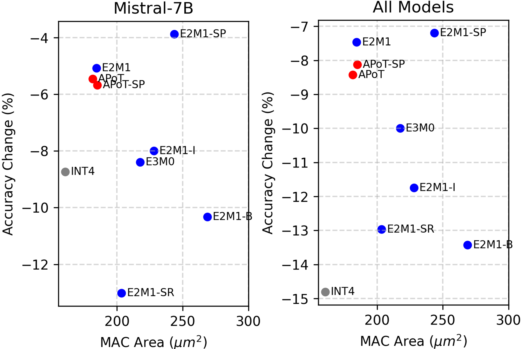
Figure 3: Quality vs. Area – Relative accuracy change from unquantized baselines averaged across zero-shot tasks. All Model results averaged across Mistral-7B, OPT-1B, OPT-6.7B, LLaMA2-7B, Phi-2, BLOOM-7B, and Yi-6B.

DNN quantization has become essential for enabling LLM applications to reach latency targets and reduce infrastructure costs. Traditionally, these quantization methods have relied on integer datatypes, yet the recent success of FP8 formats motivates further study of non-integer formats at four bits. In this work, we first profile over 30 DNNs and discover most have weights and activations that are best approximated by the Student’s t-distribution. Then, by optimizing for this distribution, we introduce Student Float (SF4), which can be used as a drop-in replacement for NF4 in memory-bound applications involving weight-only quantization. We first find it increases model quality across the most popular LLMs and then use these insights to analyze more efficient datatypes. For example, the high accuracy of E2M1 over INT4 stems from its piecewise approximation of SF4. These high-quality datatypes reduce the need for more complex algorithmic optimizations such as SmoothQuant, GPTQ, and granular subchannel quantization. This decreases the system complexity, such as maintaining SmoothQuant scales on residual branches and optimizing low block-size subchannel quantization, and it lowers the effort necessary for high-quality LLM quantization.

Finally, we introduce supernormal extensions to E2M1 and APoT to increase their model accuracies at the cost of minor increases in the system area. We map out the Pareto frontier across datatypes in terms of model accuracy and chip area. This frontier begins with INT4 with lowest accuracy but highest efficiency and extends to E2M1 with super-precision with highest accuracy and close to highest area. In particular, we find that E2M1 with supernormal support increases the accuracy of Phi-2 by up to 2.19% with 1.22% estimated chip overhead, offering a promising option to enable new quality-neutral LLM applications at four bits.

Appendix A Weight and Activation Profiling

Model	Weight		Activation
	$\nu$	KS-$\Delta$	$\nu$	KS-$\Delta$
GPT2	2.040.86	0.086	7.212.13	0.097
OPT-1B	6.682.86	0.040	5.914.08	0.117
BLOOM-560M	5.872.68	0.020	6.754.84	0.066
BLOOM-7B	10.135.96	-0.019	4.511.33	0.049
Falcon-7B	5.872.68	0.020	6.754.84	0.066
LLaMA2-7B	6.783.45	0.025	2.980.89	0.022
Yi-6B	7.264.98	0.013	2.503.30	0.036
T5-Small	11.804.01	0.004	6.742.94	0.021
FLAN-T5	13.472.40	0.004	5.341.53	0.031
Mistral-7B	1.660.67	0.049	1.672.15	0.111
Zephyr-3B	4.595.20	0.099	2.371.03	0.098
BERT	13.132.42	-0.069	6.454.35	0.034
RoBERTa	7.282.18	0.022	6.694.77	0.022
ALBERT	10.874.86	0.000	7.811.75	0.018
VGG19	5.962.24	0.016	1.810.75	0.095
ResNet18	2.710.69	0.069	10.946.20	-0.008
ResNet50	2.951.22	0.052	6.577.03	0.006
ResNet101	1.960.84	0.075	9.265.13	0.008
InceptionV3	2.610.83	0.044	12.024.62	0.002
InceptionV4	2.291.55	0.007	9.186.11	-0.039
MNASNet100	4.454.27	0.020	9.845.56	0.021
MobileNetV2	5.025.55	0.003	8.227.92	0.003
MobileNetV3	4.353.16	0.031	7.825.98	0.581
EfficientNet-B0	4.295.42	0.065	3.511.86	0.029
ConvNext-S	1.960.79	0.110	4.594.07	0.069
RegNet	2.911.78	0.075	6.122.37	0.037
ConvMixer	2.451.16	0.125	9.845.56	0.021
CoAT-Lite	2.111.87	0.050	7.295.28	-0.006
PiT-B	8.133.25	0.006	8.874.22	0.017

Table 10: Profiling – DNN distributions are better approximated by t-distributions, typically with single-digit degrees of freedom ($\nu$). The mean and variance for $\nu$ are calculated across layers. The Kolmogorov-Smirnov (KS) $\Delta$ measures the difference between the KS distance run on the best-fit normal and Student’s t-distributions. Positive values indicate a smaller distance to the t-distribution. For activation profiling, model inputs are randomly generated.

Model	Weight		Activations
	$\nu$	KS-$\Delta$	$\nu$	KS-$\Delta$
Query	9.884.78	-0.008	3.770.46	0.027
Key	9.484.85	-0.001	11.074.56	-0.002
Value	13.832.10	-0.001	9.404.33	0.002
Out	8.774.50	0.004	4.021.44	0.029
FC1	9.564.98	0.010	9.725.16	0.034
FC2	5.682.64	0.021	9.725.16	0.242
Total	9.534.72	0.004	4.661.11	0.040

Table 11: OPT-125M Profiling Breakdown – Disaggregating the profiling metrics for different layer types on OPT-125M.

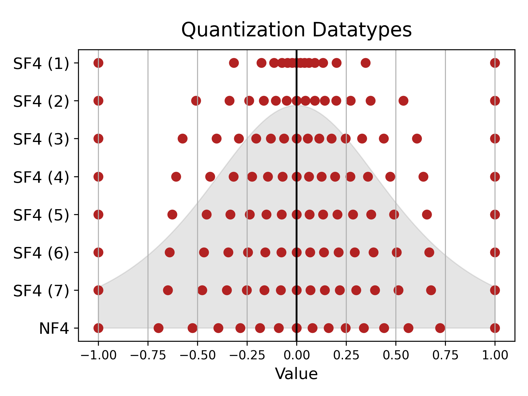
Figure 4: Degrees of Freedom – Higher degrees of freedom lead to datatypes with more spread, and in the limit, SF4 approaches NF4. Most distributions have degrees of freedom close to 5, and therefore the SF4 ($\nu=5$) datatype is used throughout Section 4.

For weights and activation profiling, we use Huggingface transformers, PyTorch torchvision, and the timm package to load models. We chose the models holistically based on historical significance, current popularity, architectural types, and diversity across tasks. This leads to including LLMs, BERT-like transformers, CNNs, RNNs, and diffusion models.

To profile the model, we iterate through the model modules and filter for nn.Linear, nn.Conv1D, and nn.Conv2D. If the weight tensors are extremely large containing hundreds of millions of entries, we randomly downsample since small studies showed this did not significantly affect the profiling results. For activation profiling, we use randomly generated inputs with the appropriate shape to match the current model.

Table 10 shows all the model profiling data, comparing between Student’s t-distributions and normal distributions. It lists the mean and variance for the degrees of freedom $\nu$ calculated across layers within the model. In addition, it shows the difference between two Kolmogorov-Smirnov distances: the first is between the profiled distributions and the best-fitting normal distribution, and the second with respect to the best-fitting Student’s t-distribution. A positive difference between the normal and t-distribution distances indicates that the t-distribution is closer, and therefore it better represents the profiled data.

The degrees of freedom and KS-$\Delta$ are shown for both the weights and activations. Overall, the activations typically have smaller degrees of freedom. For example, BLOOM-7B has an average of 10.13 for its weights and 4.51 for its activations, and FLAN-T5 has 13.47 for its weights and 5.34 for its activations. The degrees of freedom and KS-$\Delta$ are also very correlated, since a high degree of freedom indicates a distribution closer to normal. Only the models with $\nu>10$ have a negative KS-$\Delta$, which indicates this is a useful intuitive cutoff for classifying a distribution as normal.

In addition, we disaggregate the data across layer types, e.g. separating the attention layers from the linear layers in transformers. This analysis is shown in Table 11 for the OPT-125M model, which separately averages the degrees of freedom and KS-$\Delta$ for different layer types. It shows some differences between layer types, with FC2 having the lowest $\nu$, yet overall most layers are similar within their variance.

Appendix B Weight-Only

		Mistral-7B		OPT-1B		OPT-6.7B		LLaMA2-7B		Phi-2		BLOOM-7B		Yi-6B
Calib. Method		None	MSE	None	MSE	None	MSE	None	MSE	None	MSE	None	MSE	None	MSE
WikiText-2 ↓	FP32	18.01	18.01	16.41	16.41	12.28	12.28	8.79	8.79	11.05	11.05	14.71	14.71	10.21	10.21
	NF4	19.80	19.36	17.17	17.13	12.73	12.75	9.11	9.12	11.89	11.89	14.94	14.74	10.36	10.47
	SF4	19.09	19.34	17.11	17.10	12.67	12.66	9.16	9.10	11.83	11.84	14.96	14.84	10.34	10.36
	INT4	20.17	20.81	18.28	18.02	13.27	13.20	9.33	9.71	12.41	12.81	15.16	15.25	10.71	11.34
	E2M1-I	20.07	20.55	17.86	18.00	12.92	12.96	9.37	9.74	12.19	12.38	15.18	15.16	10.69	11.34
	E2M1-B	20.93	21.17	18.34	18.15	13.11	13.19	9.43	9.89	12.37	12.64	15.22	15.26	10.76	11.54
	E2M1	19.76	19.27	17.24	17.25	12.78	12.79	9.17	9.21	11.97	11.99	15.01	15.18	10.42	10.54
	+ SR	20.25	20.25	17.62	17.62	13.06	13.06	9.84	9.84	12.58	12.58	15.95	15.82	11.60	11.54
	+ SP	19.38	19.47	17.19	17.18	12.76	12.77	9.13	9.20	11.92	11.96	14.98	14.89	10.37	10.29
	E3M0	20.25	21.93	18.29	18.41	13.31	13.91	9.87	10.06	12.74	12.92	15.61	15.71	11.42	11.43
	APoT4	19.13	19.23	17.47	17.42	12.84	12.88	9.15	9.27	12.09	12.17	15.02	14.98	10.46	10.49
	+ SP	18.93	19.32	17.40	17.32	12.80	12.85	9.11	9.41	11.98	12.06	14.99	14.92	10.40	10.39

Table 12: Weight-Only WikiText-2 – All models evaluated with weight-only sub-channel quantization with block size 128. Student Float (SF4) typically outperforms NF4, and the super normal variants (SR and SP) often improve the model performance over E2M1.

Table 12 shows the additional evaluations across models on WikiText-2. As a measure of perplexity, this is most sensitive metric to model changes, as others tend to mask their changes through a classification problem (e.g. multiple choice). This table shows consistent improvement with SF4 over NF4 across models with the exception of BLOOM-7B. Results are shown with and without MSE calibration.

	EN ↑	FR ↑	DE ↑	IT ↑	ES ↑	Wiki ↓
FP32	73.92	50.69	39.51	46.09	43.57	8.791
NF4	73.20	48.20	37.53	44.50	42.67	9.105
SF4	72.35	48.79	38.54	44.81	44.44	9.163
INT4	72.06	47.45	37.26	42.87	42.60	9.333
E2M1-I	71.43	47.43	37.07	42.48	42.05	9.366
E2M1-B	70.75	47.41	36.54	42.11	41.02	9.427
E2M1	71.65	47.49	37.05	42.91	42.50	9.168
+ SR	71.07	45.27	35.14	41.45	39.36	9.842
+ SP	71.65	47.00	37.36	42.87	42.01	9.131
E3M0	69.92	45.37	35.20	42.05	40.68	9.868
APoT4	72.77	48.98	37.88	45.16	41.53	9.149
+ SP	73.22	48.75	37.55	44.34	41.57	9.109

Table 13: LLaMA2-7B Multi-Lingual – LLaMA2-7B comparison across multi-lingual LAMBADA tasks and WikiText-2. SF4 outperforms NF4 on lookup datatypes, and E2M1 with subnormal and super-precision outperforms other FP4 datatypes.

Table 13 shows the results of LLaMA2-7B on a multi-lingual version of the LAMBADA dataset. It reinforces the previous trends, which SF4 typically achieving higher accuracy and E2M1 with and without super-precision outperform other datatypes.

Appendix C GPTQ

	Channelwise		Subchannel
	RTN	GPTQ	RTN	GPTQ
NF4	-4.86	-2.48	-1.87	-1.14
SF4	-3.69	-2.49	-1.33	-1.65
INT4	-7.98	-6.45	-2.96	-2.39
E2M1-I	-6.57	-5.47	-2.67	-2.31
E2M1-B	-8.58	-5.35	-2.80	-2.46
E2M1	-3.92	-2.57	-1.40	-1.48
+ SR	-3.21	-2.19	-1.86	-1.17
+ SP	-3.85	-2.35	-0.66	-1.54
E3M0	-6.17	-4.76	-4.50	-3.64
APoT4	-4.35	-3.80	-1.90	-1.89
+ SP	-3.43	-2.91	-1.29	-1.46

Table 14: Phi-2 GPTQ – Format quality differences remain with weight-only quantization with the inclusion of more sophisticated methods like GPTQ (Frantar et al., 2023). The average accuracy drop (%) is shown, calculated across LAMBADA, HellaSwag, Winogrande, PIQA, BoolQ, and ARC-c. Round-to-nearest (RTN) quantization is the baseline and results are evaluated with and without subchannel quantization with 128-element subchannels.

We further include additional recent weight-only optimization to ensure the quality differences between formats are not sensitive to additional optimizations. GPTQ (Frantar et al., 2023) is a popular weight-only optimizer that uses the second-order Hessian information to improve quantization quality. Table 14 shows the addition of GPTQ on the Phi-2 model evaluated across the standard zero-shot task mixture: LAMBADA, HellaSwag, Winogrande, PIQA, BoolQ, and ARC-c. It uses both channelwise and subchannel quantization with subchannel size 128, which is a common choice to balance quality and performance. These results were gathered from a modified version of neural compressor that uses lookup based quantization during the GPTQ optimization step.

The table overall shows some improvement from using GPTQ, although the results are mixed across methods and benchmarks. The super-precision E2M1 formats again show their dominance across methods, with the best performing method being RTN super-precision E2M1 with only a 0.66% average decrease in accuracy across tasks.

Appendix D SmoothQuant

	Channelwise		Subchannel
	No SQ	SQ	No SQ	SQ
NF4	-41.87	-22.30	-2.65	-3.60
SF4	-25.12	-14.02	-2.82	-3.45
INT4	-52.01	-50.42	-6.27	-6.35
E2M1-I	-51.63	-51.69	-6.11	-5.60
E2M1-B	-52.68	-52.71	-7.47	-6.63
E2M1	-37.01	-20.93	-2.68	-3.44
+ SR	-25.04	-20.88	-12.28	-13.14
+ SP	-41.16	-20.03	-3.42	-3.24
E3M0	-16.17	-23.46	-10.66	-9.13
APoT4	-51.19	-48.89	-3.74	-4.23
+ SP	-51.39	-42.49	-3.50	-4.19

Table 15: LlaMA2-7B W4A4 SmoothQuant – Quality differences between formats are not changed with adding SmoothQuant (SQ). Results use either channelwise or subchannel quantization with a subchannel block size of 128. The average accuracy drop (%) is shown, calculated across LAMBADA, HellaSwag, Winogrande, PIQA, BoolQ, and ARC-c. Activation quantization is dynamic and SQ uses an alpha factor of 0.5.

With weight-only quantization, Section C confirmed that the addition of more advanced quantization algorithms did not affect relative format performance. Likewise, with four-bit weight and activation quantization (W4A4) techniques like SmoothQuant (Xiao et al., 2023) (SQ) have been proposed to improve accuracy by shifting the quantization difficulty from the activations to the weights. Originally proposed for W8A8 quantization, the same method can be applied to lower precisions as well.

Table 15 shows the results for Phi-2 with W4A4 quantization, with and without SQ applied, evaluated across LAMBADA, HellaSwag, Winogrande, PIQA, BoolQ, and ARC-c. It first confirms that subchannel quantization is essential for LLM quantization at this precision, since the average accuracy drop across tasks is close to 50% on average. It also shows that SQ does not always increase model quality, although it does on average. Since these differences are small compared to the differences among formats, this does not affect their relative quality.

Appendix E Student Float

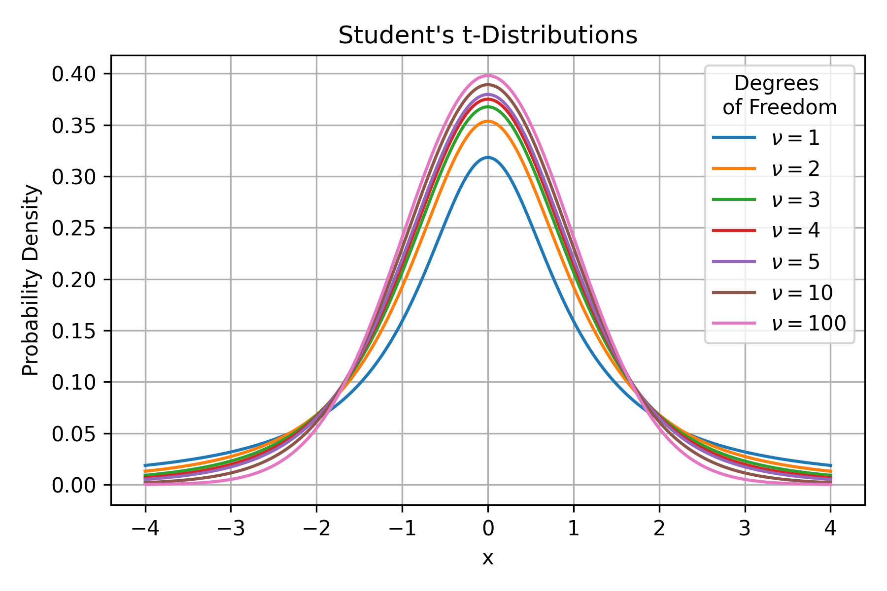
Figure 5: t-Distributions – Increasing the degrees of freedom, $\nu$, leads to more probability mass in the center, and less at the edges of the distribution. This leads to more representation in the center of the SF4 datatype, and in the limit, the NF4 datatype.

Figure 4 shows that SF4 converges to NF4 as its degrees of freedom increase to infinity. This allows testing for gradually denser datatypes toward NF4 and making comparisons to the corresponding degrees of freedom in the profiling results in Table 10. Overall, on average models approximately have $\nu=5$, which leads to the highest accuracy results across tasks.

Appendix F Datatype Values

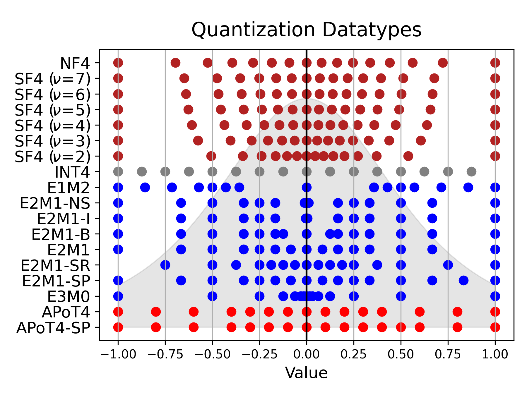
Figure 6: Datatype Shapes – The shapes of all considered datatypes, including lookup datatypes, integer, floating-point, and APoT (Li et al., 2020).

Datatype	Values
NF4	-1.000	-0.696	-0.525	-0.395	-0.284	-0.185	-0.091	0.000	0.080	0.161	0.246	0.338	0.441	0.563	0.723	1.000
SF4 ($\nu=3$)	-1.000	-0.576	-0.404	-0.292	-0.205	-0.131	-0.064	0.000	0.056	0.114	0.176	0.246	0.330	0.439	0.606	1.000
SF4 ($\nu=4$)	-1.000	-0.609	-0.436	-0.318	-0.225	-0.145	-0.071	0.000	0.062	0.126	0.194	0.270	0.359	0.472	0.638	1.000
SF4 ($\nu=5$)	-1.000	-0.628	-0.455	-0.334	-0.237	-0.153	-0.075	0.000	0.066	0.133	0.205	0.284	0.376	0.491	0.657	1.000
SF4 ($\nu=6$)	-1.000	-0.640	-0.467	-0.345	-0.246	-0.158	-0.078	0.000	0.068	0.138	0.212	0.293	0.387	0.504	0.669	1.000
INT4	-8.000	-7.000	-6.000	-5.000	-4.000	-3.000	-2.000	-1.000	0.000	1.000	2.000	3.000	4.000	5.000	6.000	7.000
E2M1-I	-6.000	-4.000	-3.000	-2.000	-1.500	-1.000	-0.062	0.000	0.062	1.000	1.500	2.000	3.000	4.000	6.000
E2M1-B	-12.000	-8.000	-6.000	-4.000	-3.000	-2.000	-0.062	0.000	0.062	2.000	3.000	4.000	6.000	8.000	12.000
E2M1-NS	-6.000	-4.000	-3.000	-2.000	-1.500	-1.000	-0.750	0.000	0.750	1.000	1.500	2.000	3.000	4.000	6.000
E2M1	-6.000	-4.000	-3.000	-2.000	-1.500	-1.000	-0.500	0.000	0.500	1.000	1.500	2.000	3.000	4.000	6.000
+ SR	-6.000	-4.000	-3.000	-2.000	-1.500	-1.000	-0.500	0.000	0.500	1.000	1.500	2.000	3.000	4.000	6.000	8.000
+ SP	-6.000	-4.000	-3.000	-2.000	-1.500	-1.000	-0.500	0.000	0.500	1.000	1.500	2.000	3.000	4.000	5.000	6.000
E3M0	-16.000	-8.000	-4.000	-2.000	-1.000	-0.500	-0.250	0.000	0.250	0.500	1.000	2.000	4.000	8.000	16.000
APoT4	-1.000	-0.800	-0.600	-0.400	-0.300	-0.200	-0.100	0.000	0.100	0.200	0.300	0.400	0.600	0.800	1.000
+ SP	-1.000	-0.800	-0.600	-0.400	-0.300	-0.200	-0.100	0.000	0.100	0.200	0.300	0.400	0.500	0.600	0.800	1.000

Table 16: Quantized Datatype Values – The specific values for each datatype across lookup, integer, floating-point, and alternative formats. Some datatypes have only 15 values, as opposed to 16 ($2^{4}$), since they include a dedicated sign bit, which leads to representations for positive and negative zero. The Student Float (SF4) formats include versions for different degrees of freedom ($\nu$), which cluster values in different ways. For floating-point formats, the Intel (Shen et al., 2023) (I-E2M1) and bitsandbytes (Dettmers et al., 2022a) (B-E2M1) versions are included as references too. Additive Powers of Two (APoT) (Li et al., 2020) is also shown which performs the sum of two logarithmic numbers. Finally, the super-precision (SP), super-range (SR), and no subnormal (NS) variants are shown for some of these formats.

This section lists the values for all the datatypes used in the evaluations in Section 4 and Section 5. In addition, it shows all of the datatypes in the same figure, including the lookup datatypes, integer, floating-point, and APoT variants.

Appendix G Additive Powers-of-Two

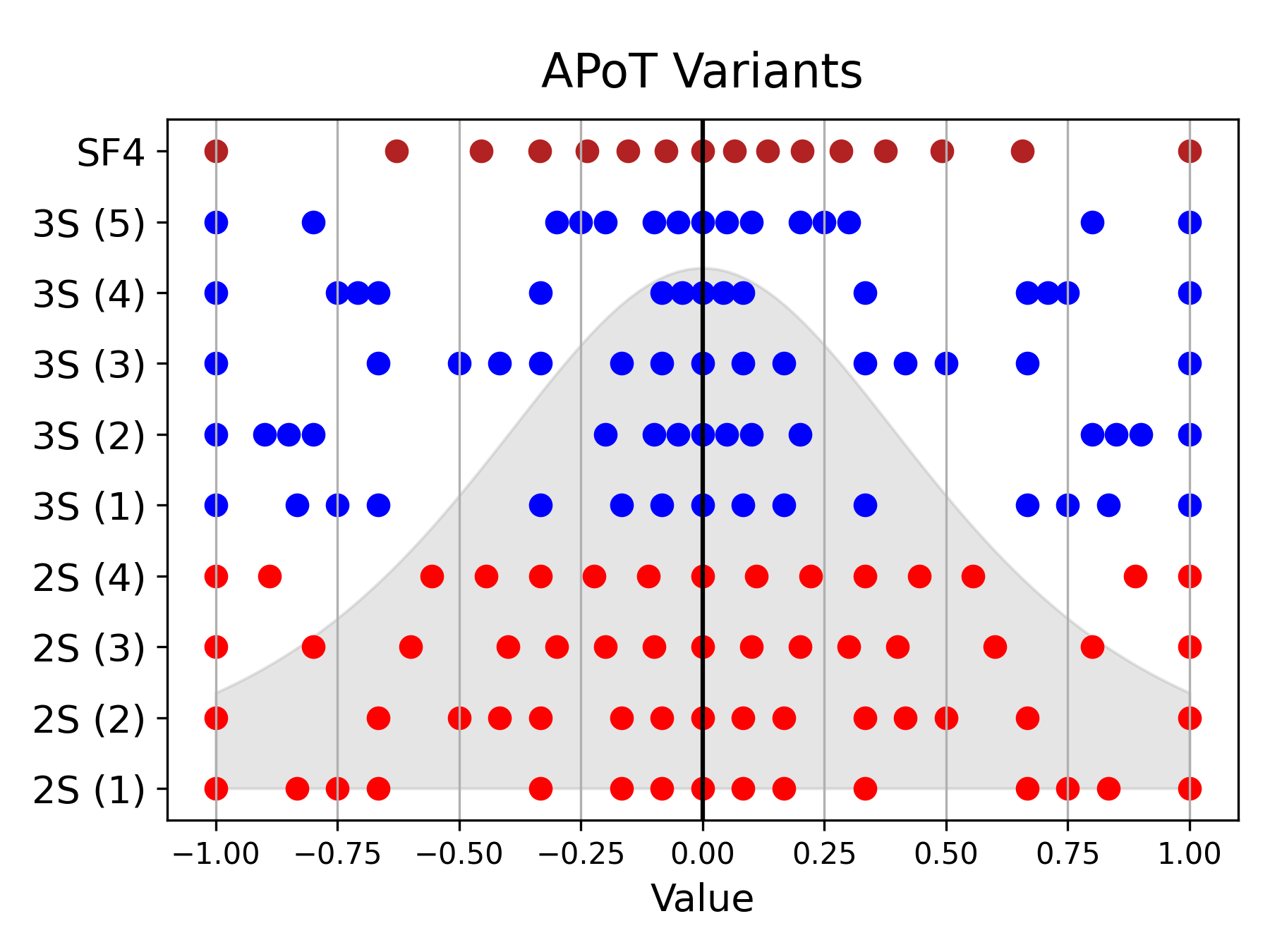
Figure 7: APoT4 Variants – Comparison across APoT4 variants with two sets (2S) and three sets (3S), where each datatype is constructed by all possible sums by taking one value from each set. For example, the 2S (3) variant used in Section 4, uses the sets $S_{1}\in\{0,2^{-1},2^{-2},2^{-4}\}$ and $S_{2}\in\{0,2^{-3}\}$. The values to construct the sets are always drawn from $\{0,2^{-1},2^{-2},2^{-4}\}$. SF4 is shown for reference.

The Additive Powers-of-Two method leads to a large search space of datatypes, where all the most reasonable variants are shown in Figure 7. These have been filtered to remove datatypes that lead to duplicate values (under-utilizing the bitspace) and different configurations that lead to the exact same datatype. This figure shows that the 2S (3) variant best approximates the SF4 datatype, and therefore in this work we focus only on this variant.

Appendix H Additional Paretos

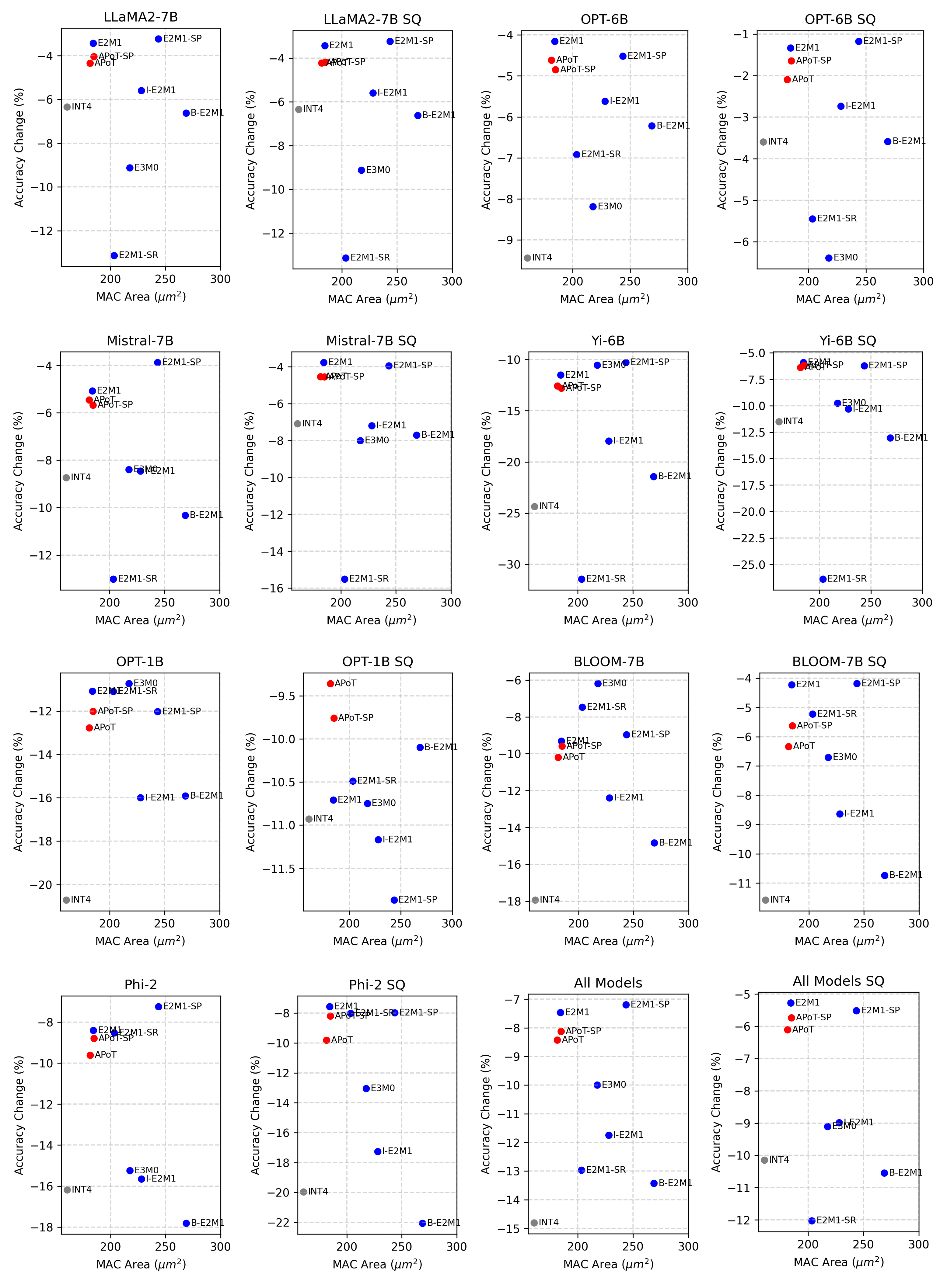
Figure 8: All Model Paretos – Relative accuracy change from unquantized baselines averaged across LAMBADA, HellaSwag, Winogrande, PIQA, BoolQ, and ARC-c. All models are quantized with W4A4 subchannel quantization with SmoothQuant (Xiao et al., 2023) included on models with the SQ label.

This section includes all of the Pareto-curves for Mistral-7B, OPT-1B, OPT-6.7B, LLaMA2-7B, Phi-2, BLOOM-7B, and Yi-6B evaluated across LAMBADA, HellaSwag, Winogrande, PIQA, BoolQ, and ARC-c. The y-axis represents the average relative accuracy change from floating-point, and the x-axis is the corresponding MAC area for the datatype.

Appendix I Additional Tables

Metric	LAMB	Hella	Wino	PIQA	BoolQ	ARC-c
BF16	73.92	57.14	69.14	78.07	77.74	43.43
NF4	72.35	56.55	69.53	76.99	77.40	42.49
SF4	73.20	56.81	69.06	77.69	78.56	43.34
INT4	72.06	56.53	69.14	77.31	76.76	42.92
I-E2M1	71.43	56.50	68.90	77.80	77.06	42.66
B-E2M1	70.75	56.54	68.98	77.58	76.73	43.34
E2M1	71.65	56.69	69.53	77.97	78.13	42.49
+ SR	71.07	54.66	66.85	76.77	73.55	42.41
+ SP	71.65	56.84	69.43	77.99	78.26	42.49
E3M0	69.92	54.61	67.64	76.55	75.32	39.59
APoT4	72.77	56.27	68.27	78.07	77.55	43.17
+ SP	73.22	56.56	68.59	77.69	77.68	43.86

Table 17: LLaMA-7B Weight-Only Subchannel 128

	LAMB	Hella	Wino	PIQA	BoolQ	ARC-c
FP32	62.57	55.84	75.45	78.78	83.21	52.56
NF4	60.47	54.66	75.22	77.42	82.81	50.85
SF4	61.28	54.75	75.30	78.13	80.76	52.56
INT4	58.59	54.51	75.61	77.69	79.14	51.02
I-E2M1	58.20	54.06	74.59	77.69	82.45	51.28
B-E2M1	58.32	54.07	75.22	77.04	82.32	50.85
E2M1	59.95	54.83	76.24	77.09	83.06	51.96
+ SR	63.24	53.32	75.06	78.40	81.38	50.17
+ SP	61.73	55.06	76.01	76.99	83.21	52.73
E3M0	54.96	52.18	74.59	78.56	80.86	50.43
APoT4	59.62	54.50	74.35	77.91	81.35	52.82
+ SP	61.09	54.66	74.27	78.35	81.71	52.90

Table 18: Phi-2 Weight-Only Subchannel 128

Metric	LAMB	Hella	Wino	PIQA	BoolQ	ARC-c
FP32	75.92	61.22	73.88	80.58	83.58	50.43
NF4	74.97	60.90	72.93	80.30	82.84	49.74
SF4	75.90	60.73	73.80	80.63	83.09	49.40
INT4	73.92	60.59	73.80	80.36	82.23	49.32
I-E2M1	74.17	60.41	72.45	80.36	82.84	48.98
B-E2M1	73.98	60.36	72.22	80.09	82.48	48.81
E2M1	74.75	60.57	73.16	80.14	82.29	48.55
+ SR	72.95	59.07	73.56	79.65	82.84	47.95
+ SP	75.41	60.96	72.93	80.36	83.46	47.78
E3M0	74.23	58.76	72.22	79.71	81.99	46.42
APoT4	75.41	60.89	73.95	80.30	83.09	47.44
+ SP	75.12	61.05	73.09	80.20	83.03	48.21

Table 19: Mistral-7B Weight-Only Subchannel 128

Metric	LAMB	Hella	Wino	PIQA	BoolQ	ARC-c
FP32	68.27	55.40	70.96	77.64	75.50	46.25
NF4	67.46	54.81	71.03	77.26	78.47	44.97
SF4	67.84	54.75	70.80	77.15	76.97	45.14
INT4	64.93	54.51	68.75	77.31	75.41	44.37
I-E2M1	64.39	54.48	71.11	77.26	75.81	44.71
B-E2M1	63.92	54.56	70.56	77.09	75.32	44.20
E2M1	66.74	54.52	69.85	76.71	76.57	45.05
+ SR	59.97	52.95	67.80	75.90	76.18	43.52
+ SP	67.38	54.83	70.56	76.71	76.27	46.50
E3M0	65.15	52.48	68.90	76.33	73.82	41.81
APoT4	68.21	55.08	70.24	77.69	77.49	45.73
+ SP	68.14	55.25	70.88	77.58	77.34	45.39

Table 20: Yi-6B Weight-Only Subchannel 128

Metric	LAMB	Hella	Wino	PIQA	BoolQ	ARC-c
FP32	57.64	46.49	64.56	72.69	62.81	30.29
NF4	57.03	45.47	62.98	72.96	63.46	30.38
SF4	57.77	45.43	64.25	72.25	62.87	29.86
INT4	56.08	45.31	63.54	73.12	63.55	29.44
I-E2M1	55.75	45.66	63.38	72.80	63.24	29.95
B-E2M1	55.64	45.47	62.90	72.96	63.21	30.20
E2M1	56.51	45.26	63.30	72.63	63.43	30.12
+ SR	50.18	44.56	62.75	72.63	61.44	30.63
+ SP	56.86	45.41	63.46	72.74	63.46	30.03
E3M0	56.47	44.36	61.25	72.47	63.67	29.78
APoT4	57.02	45.30	63.85	72.96	62.57	29.86
+ SP	57.13	45.46	63.22	72.47	62.72	29.86

Table 21: BLOOM-7B Weight-Only Subchannel 128

Metric	LAMB	Hella	Wino	PIQA	BoolQ	ARC-c
FP32	67.69	50.49	65.43	76.28	66.06	30.72
NF4	67.88	49.34	64.25	76.22	65.99	30.63
SF4	68.02	49.58	64.96	75.90	64.04	30.03
INT4	63.92	49.02	63.93	75.63	65.23	31.23
I-E2M1	67.49	49.44	64.17	76.22	65.84	30.20
B-E2M1	66.97	49.42	63.06	76.55	67.06	31.14
E2M1	67.84	49.15	64.17	76.06	66.02	30.63
+ SR	67.26	48.48	64.48	75.14	63.46	29.44
+ SP	67.24	49.29	63.77	76.17	65.96	30.38
E3M0	62.64	48.16	63.38	74.65	65.96	30.12
APoT4	66.08	49.64	64.64	75.79	65.02	30.63
+ SP	65.92	49.59	64.96	75.95	64.31	31.06

Table 22: OPT-6B Weight-Only Subchannel 128

		LAMB	Hella	Wino	PIQA	BoolQ	ARC-c
No SmoothQuant	FP32	68.27	55.4	70.96	77.64	75.5	46.25
	NF4	51.17	51.34	63.77	74.21	71.93	40.70
	SF4	55.29	51.58	64.33	74.59	73.03	40.44
	INT4	31.4	46.14	56.2	71.49	58.84	34.81
	I-E2M1	42.36	48.89	60.14	71.93	64.16	36.77
	B-E2M1	34.52	47.16	55.64	70.78	63.64	37.80
	E2M1	49.62	50.93	63.61	73.23	72.02	40.19
	+ SR	23.50	41.69	55.33	65.13	63.12	25.94
	+ SP	48.13	50.80	63.77	74.21	66.61	40.36
	E3M0	59.07	49.19	64.80	73.07	69.97	38.48
	APoT4	47.18	50.42	62.35	74.48	69.05	41.21
	+ SP	48.13	50.80	63.77	74.21	66.61	40.36
SmoothQuant	NF4	61.81	53.40	65.59	74.92	72.75	43.94
	SF4	64.72	53.48	66.93	76.61	73.24	44.45
	INT4	51.85	51.13	63.93	74.65	68.29	39.76
	I-E2M1	53.58	51.55	63.38	74.48	68.20	42.06
	B-E2M1	51.39	50.93	62.27	73.78	67.25	38.23
	E2M1	61.91	53.13	65.59	75.84	69.45	44.28
	+ SR	34.97	44.82	57.46	65.51	65.47	26.62
	+ SP	59.25	53.37	66.69	75.35	70.70	43.94
	E3M0	59.77	49.82	65.35	74.16	72.08	37.37
	APoT4	58.80	53.07	67.64	74.43	72.81	42.58
	+ SP	59.25	53.37	66.69	75.35	70.70	43.94

Table 23: Yi-6B W4A4 Subchannel 128

		LAMB	Hella	Wino	PIQA	BoolQ	ARC-c
No SmoothQuant	FP32	57.64	46.49	64.56	72.69	62.81	30.29
	NF4	44.23	42.69	59.12	69.86	60.55	29.18
	SF4	48.98	43.24	59.04	70.29	58.87	29.01
	INT4	31.15	39.91	54.38	67.79	54.16	26.88
	I-E2M1	41.8	42.04	55.33	68.72	57.22	27.65
	B-E2M1	36.48	40.83	54.78	67.95	57.77	27.13
	E2M1	44.21	42.37	59.51	70.02	59.51	28.16
	+ SR	48.22	41.51	57.22	70.62	61.96	29.61
	+ SP	44.58	42.82	58.48	70.73	59.69	28.41
	E3M0	52.55	42.48	56.51	70.24	62.48	29.27
	APoT4	40.15	41.95	58.88	70.40	60.98	28.41
	+SP	41.35	41.98	59.19	70.62	59.82	29.18
SmoothQuant	NF4	52.90	44.50	60.69	71.38	61.65	28.84
	SF4	55.29	45.06	61.09	72.31	63.64	29.86
	INT4	41.72	41.72	56.83	69.53	57.13	28.41
	I-E2M1	47.08	42.21	57.06	69.91	61.50	28.24
	B-E2M1	43.76	41.06	56.67	69.86	61.13	27.30
	E2M1	53.77	44.52	60.46	71.76	61.74	28.75
	+ SR	52.94	42.11	58.41	71.06	63.30	29.44
	+ SP	51.09	43.92	58.98	70.78	59.62	30.12
	E3M0	51.93	42.4	57.93	69.8	62.84	28.07
	APoT	50.11	43.81	58.33	70.62	59.48	29.86
	+ SP	51.09	43.92	58.98	70.78	59.62	30.12

Table 24: BLOOM-7B W4A4 Subchannel 128

		LAMB	Hella	Wino	PIQA	BoolQ	ARC-c
No SmoothQuant	FP32	73.92	57.14	69.14	78.07	77.74	43.43
	NF4	73.03	55.57	67.09	76.55	75.96	41.38
	SF4	72.21	55.28	66.69	76.93	75.72	41.81
	INT4	69.92	53.76	65.27	75.79	69.88	40.10
	I-E2M1	69.55	54.33	65.11	75.57	70.34	40.27
	B-E2M1	68.31	53.65	62.43	74.81	70.0	40.27
	E2M1	72.21	55.61	67.01	76.39	76.24	41.72
	+ SR	63.96	48.91	61.01	73.18	70.18	35.58
	+ SP	72.64	54.79	66.61	76.66	73.88	41.38
	E3M0	65.03	51.29	62.35	74.43	69.42	36.26
	APoT4	72.79	55.01	65.82	76.39	74.07	41.04
	+ SP	72.64	54.79	66.61	76.66	73.88	41.38
SmoothQuant	NF4	72.50	55.22	66.54	76.66	74.28	40.70
	SF4	71.90	55.09	66.06	77.04	75.35	41.04
	INT4	70.35	54.07	65.43	75.79	68.90	39.85
	I-E2M1	70.39	53.92	66.22	76.28	72.11	39.33
	B-E2M1	70.44	53.73	64.96	75.03	69.88	39.51
	E2M1	72.21	55.10	65.9	76.93	74.71	41.38
	+ SR	64.25	47.97	61.33	73.01	68.96	34.47
	+ SP	71.78	55.13	65.75	77.37	73.94	39.93
	E3M0	66.74	51.16	64.25	75.68	71.71	36.18
	APoT4	71.82	54.87	66.22	76.39	73.76	40.36
	+ SP	71.78	55.13	65.75	77.37	73.94	39.93

Table 25: LLaMA-7B W4A4 Subchannel 128

		LAMB	Hella	Wino	PIQA	BoolQ	ARC-c
No SmoothQuant	FP32	75.90	61.22	73.88	80.58	83.58	50.43
	NF4	72.02	59.66	68.11	79.38	80.64	47.18
	SF4	73.47	59.83	69.38	79.71	81.10	46.25
	INT4	64.99	58.11	67.01	77.69	76.82	44.37
	I-E2M1	66.41	57.23	68.59	78.35	74.98	44.62
	B-E2M1	64.22	57.19	66.22	77.09	75.29	42.66
	E2M1	72.0	59.56	69.85	79.05	79.60	45.14
	+ SR	65.01	51.32	66.46	75.35	76.02	39.33
	+ SP	70.83	59.66	69.30	78.56	79.57	44.71
	E3M0	70.87	55.48	66.14	77.86	80.12	42.15
	APoT4	71.2	59.29	68.43	79.38	79.33	45.65
	+ SP	70.83	59.66	69.30	78.56	79.57	44.71
SmoothQuant	NF4	73.86	59.17	71.19	79.54	80.58	46.42
	SF4	74.50	59.64	71.74	79.98	82.20	46.67
	INT4	68.41	57.91	68.41	77.89	77.52	45.76
	I-E2M1	68.97	58.54	68.27	78.56	76.12	45.05
	B-E2M1	68.91	57.86	68.90	78.45	75.38	44.20
	E2M1	73.63	59.45	71.98	79.92	79.91	45.90
	+ SR	64.93	50.29	65.75	75.3	72.05	35.58
	+ SP	73.67	59.63	69.14	79.43	79.88	45.65
	E3M0	71.53	55.82	66.77	77.09	79.42	43.09
	APoT4	73.67	59.37	69.69	78.67	79.42	46.25
	+ SP	73.67	59.63	69.14	79.43	79.88	45.65

Table 26: Mistral-7B W4A4 Subchannel 128

		LAMB	Hella	Wino	PIQA	BoolQ	ARC-c
No SmoothQuant	FP32	57.89	41.54	59.51	71.71	57.83	23.38
	NF4	40.13	36.57	57.14	66.16	52.08	22.95
	SF4	41.98	37.27	55.33	66.54	51.38	22.78
	INT4	28.06	32.65	53.43	61.92	47.83	20.99
	I-E2M1	39.10	35.50	52.80	65.02	46.27	21.42
	B-E2M1	36.25	34.28	54.78	63.33	45.90	23.29
	E2M1	39.82	36.71	57.14	65.56	53.06	22.70
	+ SR	40.62	37.16	54.62	68.01	51.90	22.78
	+ SP	37.55	35.66	56.04	65.89	54.37	22.70
	E3M0	44.13	37.82	54.46	67.74	50.98	22.01
	APoT4	37.69	35.61	57.54	64.91	54.16	21.42
	+ SP	37.55	35.66	56.04	65.89	54.37	22.70
SmoothQuant	NF4	44.75	38.11	54.46	67.85	49.63	23.63
	SF4	43.61	38.02	57.30	67.41	49.33	22.78
	INT4	42.42	37.22	54.46	66.81	52.57	22.44
	I-E2M1	43.47	37.03	55.72	66.05	50.55	22.35
	B-E2M1	43.37	36.99	56.67	65.94	50.43	23.63
	E2M1	43.64	37.84	57.85	67.03	47.55	22.53
	+ SR	40.02	37.27	57.06	68.12	53.46	22.18
	+ SP	40.91	37.77	57.70	67.85	51.68	23.12
	E3M0	42.34	37.87	55.17	67.52	52.57	21.84
	APoT4	41.72	37.97	57.54	68.34	51.53	23.21
	+ SP	40.91	37.77	57.70	67.85	51.68	23.12

Table 27: OPT-1B W4A4 Subchannel 128

		LAMB	Hella	Wino	PIQA	BoolQ	ARC-c
No SmoothQuant	FP32	67.69	50.49	65.43	76.28	66.06	30.72
	NF4	64.89	47.86	62.75	74.54	63.21	29.01
	SF4	65.57	47.81	63.54	74.37	62.20	27.99
	INT4	53.15	44.98	60.46	72.8	62.84	28.50
	I-E2M1	62.41	47.76	60.69	73.99	62.60	29.18
	B-E2M1	60.39	47.04	61.01	73.78	63.00	29.18
	E2M1	65.22	47.39	62.75	74.32	64.10	29.01
	+ SR	62.47	46.09	59.67	73.99	63.52	27.82
	+ SP	61.73	47.28	62.04	73.88	63.82	30.03
	E3M0	57.23	45.32	60.77	72.74	62.94	28.58
	APoT4	61.40	47.56	62.43	75.14	63.39	29.95
	+ SP	61.73	47.28	62.04	73.88	63.82	30.03
SmoothQuant	NF4	67.79	49.22	63.06	75.24	65.38	30.03
	SF4	68.29	49.24	63.85	75.14	64.74	30.46
	INT4	66.72	48.8	63.22	74.10	62.57	29.10
	I-E2M1	65.55	48.64	62.83	74.59	65.29	30.03
	B-E2M1	65.94	48.40	61.72	74.27	63.06	30.12
	E2M1	68.27	49.23	63.69	75.19	64.71	30.63
	+ SR	64.62	46.36	60.22	74.81	64.37	28.41
	+ SP	67.75	49.64	64.25	74.81	62.87	30.08
	E3M0	61.96	47.30	60.93	73.50	62.6	28.33
	APoT	67.26	49.56	64.09	75.30	62.32	30.38
	+ SP	67.75	49.64	64.25	74.81	62.87	30.08

Table 28: OPT-6B W4A4 Subchannel 128

		LAMB	Hella	Wino	PIQA	BoolQ	ARC-c
No SmoothQuant	FP32	62.57	55.84	75.45	78.78	83.21	52.56
	NF4	52.20	51.63	71.03	76.93	74.62	49.74
	SF4	53.06	51.22	71.82	75.08	79.88	50.60
	INT4	41.18	47.4	67.48	74.37	66.97	46.16
	I-E2M1	43.18	47.4	67.01	75.35	66.73	45.99
	B-E2M1	39.82	46.5	67.88	74.43	66.64	42.92
	E2M1	49.66	51.19	71.82	75.30	78.29	49.23
	+SR	51.81	49.40	73.56	75.73	78.47	47.10
	+ SP	51.19	50.85	69.46	76.50	77.58	49.32
	E3M0	42.15	47.63	66.61	74.05	72.81	45.22
	APoT4	49.58	50.25	69.85	76.77	75.60	48.46
	+ SP	51.19	50.85	69.46	76.50	77.58	49.32
SmoothQuant	NF4	52.98	51.74	71.82	75.73	79.72	49.23
	SF4	55.33	51.53	71.82	76.44	80.92	49.74
	INT4	31.94	46.57	64.96	72.03	69.45	44.54
	I-E2M1	36.97	47.85	67.88	72.63	67.37	46.50
	B-E2M1	31.13	45.91	64.56	72.58	66.97	40.70
	E2M1	51.68	51.33	71.03	76.28	77.92	50.17
	+ SR	52.78	49.39	72.93	76.39	78.01	48.21
	+ SP	49.95	50.86	71.74	74.92	81.25	48.38
	E3M0	49.41	47.51	69.14	74.70	71.41	44.88
	APoT4	47.86	50.49	70.40	75.14	79.11	47.53
	+ SP	49.95	50.86	71.74	74.92	81.25	48.38

Table 29: Phi-2 W4A4 Subchannel 128

References

- Alsuhli et al. (2023) Alsuhli, G., Sakellariou, V., Saleh, H., Al-Qutayri, M., Mohammad, B., and Stouraitis, T. Number systems for deep neural network architectures: A survey. arxiv, 2023.
- Banner et al. (2018) Banner, R., Nahshan, Y., Hoffer, E., and Soudry, D. Aciq: analytical clipping for integer quantization of neural networks. arxiv, 2018.
- Bisk et al. (2020) Bisk, Y., Zellers, R., Bras, R. L., Gao, J., and Choi, Y. Piqa: Reasoning about physical commonsense in natural language. Conf. on Artificial Intell., 2020.
- Cai et al. (2020) Cai, Y., Yao, Z., Dong, Z., Gholami, A., Mahoney, M. W., and Keutzer, K. Zeroq: A novel zero shot quantization framework. CVPR, 2020.
- Chen et al. (2019) Chen, Y.-H., Yang, T.-J., Emer, J., and Sze, V. Eyeriss v2: A flexible accelerator for emerging deep neural networks on mobile devices. Journal of Emerging and Selected Topics in Circuits and Systems, 2019.
- Clark et al. (2019) Clark, C., Lee, K., Chang, M.-W., Kwiatkowski, T., Collins, M., and Toutanova, K. Boolq: Exploring the surprising difficulty of natural yes/no questions. North. American. Assoc. for Comp. Linguistics, 2019.
- Dai et al. (2021) Dai, S., Venkatesan, R., Ren, H., Zimmer, B., Dally, W. J., and Khailany, B. Vs-quant: Per-vector scaled quantization for accurate low-precision neural network inference. MLSys, 2021.
- Dettmers et al. (2022a) Dettmers, T., Lewis, M., Belkada, Y., and Zettlemoyer, L. Llm.int8(): 8-bit matrix multiplication for transformers at scale. NeurIPS, 2022a.
- Dettmers et al. (2022b) Dettmers, T., Lewis, M., Shleifer, S., and Zettlemoyer, L. 8-bit optimizers via block-wise quantization. ICLR, 2022b.
- Dettmers et al. (2023) Dettmers, T., Pagnoni, A., Holtzman, A., and Zettlemoyer, L. Qlora: Efficient finetuning of quantized llms. NeurIPS, 2023.
- Devlin et al. (2019) Devlin, J., Chang, M.-W., Lee, K., and Toutanova, K. Bert: Pre-training of deep bidirectional transformers for language understanding. North. American. Assoc. for Comp. Linguistics, 2019.
- Dotzel et al. (2024) Dotzel, J., Wu, G., Li, A., Umar, M., Ni, Y., Abdelfattah, M. S., Zhang, Z., Cheng, L., Dixon, M. G., Jouppi, N. P., Le, Q. V., and Li, S. Fliqs: One-shot mixed-precision floating-point and integer quantization search. AutoML, 2024.
- Frantar et al. (2023) Frantar, E., Ashkboos, S., Hoefler, T., and Alistarh, D. Gptq: Accurate post-training quantization for generative pre-trained transformers. NeurIPS, 2023.
- Guo et al. (2022) Guo, C., Zhang, C., Leng, J., Liu, Z., Yang, F., Liu, Y., Guo, M., and Zhu, Y. Ant: Exploiting adaptive numerical data type for low-bit deep neural network quantization. Int. Symp. on Micro Arch., 2022.
- Hao et al. (2021) Hao, C., Dotzel, J., Xiong, J., Benini, L., Zhang, Z., and Chen, D. Enabling design methodologies and future trends for edge ai: Specialization and codesign. IEEE Design & Test, 2021.
- He et al. (2015) He, K., Zhang, X., Ren, S., and Sun, J. Deep residual learning for image recognition. CVPR, 2015.
- Huang et al. (2017) Huang, G., Liu, Z., van der Maaten, L., and Weinberger, K. Q. Densely connected convolutional networks. CVPR, 2017.
- Jiang et al. (2023) Jiang, A. Q., Sablayrolles, A., Mensch, A., Bamford, C., Chaplot, D. S., de las Casas, D., Bressand, F., Lengyel, G., Lample, G., Saulnier, L., Lavaud, L. R., Lachaux, M.-A., Stock, P., Scao, T. L., Lavril, T., Wang, T., Lacroix, T., and Sayed, W. E. Mistral 7b. arxiv, 2023.
- Jouppi et al. (2021) Jouppi, N. P., Hyun Yoon, D., Ashcraft, M., Gottscho, M., Jablin, T. B., Kurian, G., Laudon, J., Li, S., Ma, P., Ma, X., Norrie, T., Patil, N., Prasad, S., Young, C., Zhou, Z., and Patterson, D. Ten lessons from three generations shaped google’s tpuv4i : Industrial product. Int. Conf. on Computer Arch., 2021.
- Jouppi et al. (2023) Jouppi, N. P., Kurian, G., Li, S., Ma, P., Nagarajan, R., Nai, L., Patil, N., Subramanian, S., Swing, A., Towles, B., Young, C., Zhou, X., Zhou, Z., and Patterson, D. Tpu v4: An optically reconfigurable supercomputer for machine learning with hardware support for embeddings. Int. Conf. on Computer Arch., 2023.
- Kazemi et al. (2023) Kazemi, M., Kim, N., Bhatia, D., Xu, X., and Ramachandran, D. Lambada: Backward chaining for automated reasoning in natural language. Assoc. for Comp. Linguistics, 2023.
- Kuzmin et al. (2022) Kuzmin, A., Van Baalen, M., Ren, Y., Nagel, M., Peters, J., and Blankevoort, T. Fp8 quantization: The power of the exponent. NeurIPS, 2022.
- Kuzmin et al. (2023) Kuzmin, A., Nagel, M., van Baalen, M., Behboodi, A., and Blankevoort, T. Pruning vs quantization: Which is better? NeurIPS, 2023.
- Li et al. (2020) Li, Y., Dong, X., and Wang, W. Additive powers-of-two quantization: An efficient non-uniform discretization for neural networks. ICLR, 2020.
- Li et al. (2023) Li, Y., Bubeck, S., Eldan, R., Giorno, A. D., Gunasekar, S., and Lee, Y. T. Textbooks are all you need ii: phi-1.5 technical report. arxiv, 2023.
- Liu et al. (2023) Liu, J., Gong, R., Wei, X., Dong, Z., Cai, J., and Zhuang, B. Qllm: Accurate and efficient low-bitwidth quantization for large language models. arxiv, 2023.
- Micikevicius et al. (2022) Micikevicius, P., Stosic, D., Burgess, N., Cornea, M., Dubey, P., Grisenthwaite, R., Ha, S., Heinecke, A., Judd, P., Kamalu, J., et al. Fp8 formats for deep learning. arXiv preprint arXiv:2209.05433, 2022.
- Miyashita et al. (2016) Miyashita, D., Lee, E. H., and Murmann, B. Convolutional neural networks using logarithmic data representation. arxiv, 2016.
- Moskvichev et al. (2023) Moskvichev, A., Odouard, V. V., and Mitchell, M. The conceptarc benchmark: Evaluating understanding and generalization in the arc domain. Trans. on Machine Learning, 2023.
- Nagel et al. (2019) Nagel, M., van Baalen, M., Blankevoort, T., and Welling, M. Data-free quantization through weight equalization and bias correction. ICCV, 2019.
- Rouhani (2023) Rouhani, B. Next-generation narrow precision data formats for ai. online, 2023. URL https://www.opencompute.org/blog/amd-arm-intel-meta-...
- Rouhani et al. (2023) Rouhani, B., Zhao, R., Elango, V., Shafipour, R., Hall, M., Mesmakhosroshahi, M., More, A., Melnick, L., Golub, M., Varatkar, G., Shao, L., Kolhe, G., Melts, D., Klar, J., L’Heureux, R., Perry, M., Burger, D., Chung, E., Deng, Z., Naghshineh, S., Park, J., and Naumov, M. With shared microexponents, a little shifting goes a long way. Int. Conf. on Computer Arch., 2023.
- Sakaguchi et al. (2019) Sakaguchi, K., Bras, R. L., Bhagavatula, C., and Choi, Y. Winogrande: An adversarial winograd schema challenge at scale. arxiv, 2019.
- Scao et al. (2023) Scao, T. L., Fan, A., Akiki, C., Pavlick, E., Ilić, S., Hesslow, D., Castagné, R., and Luccioni, A. S. Bloom: A 176b-parameter open-access multilingual language model. arxiv, 2023.
- Shao et al. (2023) Shao, W., Chen, M., Zhang, Z., Xu, P., Zhao, L., Li, Z., Zhang, K., Gao, P., Qiao, Y., and Luo, P. Omniquant: Omnidirectionally calibrated quantization for large language models. arxiv, 2023.
- Shen et al. (2023) Shen, H., Mellempudi, N., He, X., Gao, Q., Wang, C., and Wang, M. Efficient post-training quantization with fp8 formats. arxiv, 2023.
- Touvron et al. (2023) Touvron, H., Martin, L., Stone, K., Albert, P., Almahairi, A., Babaei, Y., Bashlykov, N., Batra, S., and Bhargava, P. Llama 2: Open foundation and fine-tuned chat models. arxiv, 2023.
- Wei et al. (2022) Wei, J., Bosma, M., Zhao, V. Y., Guu, K., Yu, A. W., Lester, B., Du, N., Dai, A. M., and Le, Q. V. Finetuned language models are zero-shot learners. ICLR, 2022.
- Wolf et al. (2020) Wolf, T., Debut, L., Sanh, V., Chaumond, J., Delangue, C., Moi, A., Cistac, P., Rault, T., Louf, R., Funtowicz, M., Davison, J., Shleifer, S., von Platen, P., Ma, C., Jernite, Y., Plu, J., Xu, C., Scao, T. L., Gugger, S., Drame, M., Lhoest, Q., and Rush, A. M. Transformers: State-of-the-art natural language processing. Association for Computational Linguistics, 2020.
- Xiao et al. (2023) Xiao, G., Lin, J., Seznec, M., Wu, H., Demouth, J., and Han, S. Smoothquant: Accurate and efficient post-training quantization for large language models. ICML, 2023.
- Zellers et al. (2019) Zellers, R., Holtzman, A., Bisk, Y., Farhadi, A., and Choi, Y. Hellaswag: Can a machine really finish your sentence? Assoc. for Comp. Linguistics, 2019.
- Zhang et al. (2022) Zhang, S., Roller, S., Goyal, N., Artetxe, M., Chen, M., Chen, S., Dewan, C., Diab, M., Li, X., Lin, X. V., Mihaylov, T., Ott, M., Shleifer, S., Shuster, K., Simig, D., Koura, P. S., Sridhar, A., Wang, T., and Zettlemoyer, L. Opt: Open pre-trained transformer language models. arxiv, 2022.
- Zhang et al. (2023a) Zhang, Y., Garg, A., Cao, Y., Łukasz Lew, Ghorbani, B., Zhang, Z., and Firat, O. Binarized neural machine translation. NeurIPS, 2023a.
- Zhang et al. (2023b) Zhang, Y., Zhao, L., Cao, S., Wang, W., Cao, T., Yang, F., Yang, M., Zhang, S., and Xu, N. Integer or floating point? new outlooks for low-bit quantization on large language models. arxiv, 2023b.
- Zhao et al. (2019) Zhao, R., Hu, Y., Dotzel, J., De Sa, C., and Zhang, Z. Improving Neural Network Quantization without Retraining using Outlier Channel Splitting. ICML, June 2019.
- Zhao et al. (2023) Zhao, Y., Lin, C.-Y., Zhu, K., Ye, Z., Chen, L., Zheng, S., Ceze, L., Krishnamurthy, A., Chen, T., and Kasikci, B. Atom: Low-bit quantization for efficient and accurate llm serving. arxiv, 2023.