Structure-Preserving Network Compression Via Low-Rank Induced Training Through Linear Layers Composition

Abstract

Deep Neural Networks (DNNs) have achieved remarkable success in addressing many previously unsolvable tasks. However, the storage and computational requirements associated with DNNs pose a challenge for deploying these trained models on resource-limited devices. Therefore, a plethora of compression and pruning techniques have been proposed in recent years. Low-rank decomposition techniques are among the approaches most utilized to address this problem. Compared to post-training compression, compression-promoted training is still under-explored. In this paper, we present a theoretically-justified novel approach, termed Low-Rank Induced Training (LoRITa), that promotes low-rankness through the composition of linear layers and compresses by using singular value truncation. This is achieved without the need to change the structure at inference time or require constrained and/or additional optimization, other than the standard weight decay regularization. Moreover, LoRITa eliminates the need to (i) initialize with pre-trained models and (ii) specify rank selection prior to training. Our experimental results (i) demonstrate the effectiveness of our approach using MNIST on Fully Connected Networks, CIFAR10 on Vision Transformers, and CIFAR10/100 on Convolutional Neural Networks, and (ii) illustrate that we achieve either competitive or SOTA results when compared to leading structured pruning methods in terms of FLOPs and parameters drop.

1 INTRODUCTION

In recent years, the rapid progress of machine learning has sparked substantial interest, particularly in the realm of Deep Neural Networks (DNNs), utilizing architectures such as Fully Connected Networks (FCNs) [30], Convolutional Neural Networks (CNN) [18], and Transformers [37]. DNNs have demonstrated remarkable performance across diverse tasks, including classification [6], image reconstruction [28], object recognition [26], natural language processing [37], and image generation [39]. However, the extensive storage and computational requirements of these models hinder their application in resource-limited devices. Addressing these challenges has become a focal point in recent research efforts within the context of a variety of model compression algorithms [20, 25].

Model compression techniques, based on their core strategies, can be classified into parameter quantization [16], knowledge distillation [11], lightweight model design [41], model pruning [9], and low-rank decomposition [23]. This paper specifically delves into low-rank training, partially falling under the latter category. Our approach aims to achieve a low-rank model directly through training from random initialization.

The post-training low-rank decomposition algorithms for network compression necessitate pre-trained weights [25]. In contrast, existing low-rank training methods require structural alterations to the network architecture, the specification of a pre-defined rank during training, and/or additional constraints or iterations in the training process.

In this paper, we introduce Low-Rank Induced Training (LoRITa), a novel approach that promotes low-rankness through (i) the overparameterization of layers to be compressed by linear composition and (ii) Singular Value Decomposition (SVD) post-training truncation. Unlike the well-known Low-Rank Adaptation (LoRA) method [12], our method eliminates the need for initializing with pre-trained models. LoRITa uses weight decay, the commonly chosen regularizer, for training models.

Contributions: we summarize our contributions as follows.

• We introduce a novel method that combines low-rank promoted training through linear layer composition with post-training singular value truncation on the product of composed trained weights.

• We provide theoretical justification for the low-rank nature of LoRITa-trained models by showing that standard weight decay regularization naturally imposes low-rankness to models with linear layer composition before activation.

• Through extensive experiments conducted on DNN-based image classification tasks across different FCNs, CNNs, and ViTs architectures, using MNIST, CIFAR10, and CIFAR100 datasets, we demonstrate the efficacy of our algorithm. Furthermore, as compared to leading structured pruning methods, we show that LoRITa trained models achieve either competitive or SOTA results in term of FLOPs reduction and parameters drop.

Organization: Section 2 dicusses prior arts that are related to our work. Section 3 introduces the notation, SVD, and the layers we consider. Our proposed method, LoRITa, along with its theoretical foundations, is presented in Section 4. Section 5 presents the experimental results, followed by discussing the conclusions in Section 6.

2 Related Work

In the past decade, numerous methods have been proposed in the realm of DNN compression, employing techniques such as low-rank decomposition or model pruning. Recent survey papers, such as Li et al. [20], Marinó et al. [25], offer comprehensive overviews. This section aims to survey recent works closely related to our method. Specifically, we explore papers focused on (i) post-training low-rank compression methods, (ii) low-rank training approaches, (iii) structured pruning methods, and (iv) linear layers composition for over-parameterized training.

Post-training Low-Rank Compression Methods: As an important compression strategy, low-rank compression seeks to utilize low-rank decomposition techniques for factorizing the original trained full-rank DNN model into smaller matrices or tensors. This process results in notable storage and computational savings (refer to Section 4 in Li et al. [20]). In the work by Yu et al. [40], pruning methods were combined with SVD, requiring feature reconstruction during both the training and testing phases. Another approach, presented in Lin et al. [23], treated the convolution kernel as a 3D tensor, considering the fully connected layer as either a 2D matrix or a 3D tensor. Low-rank filters were employed to expedite convolutional operations. For instance, using tensor products, a high-dimensional discrete cosine transform (DCT) and wavelet systems were constructed from 1D DCT transforms and 1D wavelets, respectively. While our method and the aforementioned approaches utilize low-rank decomposition and maintain the network structure in inference, a notable distinction lies in our approach being a training method that promotes low-rankness through the composition of linear layers. It is important to emphasize that any low-rank-based post-training compression technique can be applied to a DNN trained with LoRITa. This will be demonstrated in our experimental results, particularly with the utilization of two singular-value truncation methods.

Low-Rank Promoted Training Methods: Here, we review methods designed to promote low-rankness in DNN training. These approaches typically involve employing one or a combination of various techniques, such as introducing structural modifications (most commonly under-parameterization), encoding constraints within the training optimization process, or implementing custom and computationally-intensive regularization techniques such as the use of Bayesian estimator [7], iterative SVD [5], or the implementation of partially low-rank training [38]. The study presented in Kwon et al. [17] introduces an approach leveraging SVD compression for over-parameterized DNNs through low-dimensional learning dynamics inspired by a theoretical study on deep linear networks. The authors identify a low-dimensional structure within weight matrices across diverse architectures. Notably, the post-training compression exclusively targets the linear layers appended to the FCN, necessitating a specialized initialization. More importantly, a pre-specified rank is required, posing a challenge as finding the optimal combination of ranks for all layers is a difficult problem. In comparison, our work shares similarities as it employs a composition of multiple matrices. However, our approach encompasses all weight matrices, attention layer weights, and convolutional layers, providing a more comprehensive treatment of DNN architectures. The study conducted by Tai et al. Tai et al. [34] introduced an algorithm aimed at computing the low-rank tensor decomposition to eliminate redundancy in convolution kernels. Additionally, the authors proposed a method for training low-rank-constrained CNNs from scratch. This involved parameterizing each convolutional layer as a composition of two convolutional layers, resulting in a CNN with more layers than the original. The training algorithm for low-rank constrained CNNs required enforcing orthogonality-based regularization and additional updates. Notably, their approach did not extend to attention layers in ViTs and fully connected weight matrices. Moreover, during testing, unlike our method, their approach necessitates the presence of additional CNN layers. In a recent contribution by Sui et al. [33], a low-rank training approach was proposed to achieve high accuracy, high compactness, and low-rank CNN models. The method introduces a structural change in the convolutional layer, employing under-parameterization. Besides altering the structure, this method requires low-rank initialization and imposes orthogonality constraints during training. It is noteworthy that LoRITa, in contrast, not only preserves the existing structure at inference time but also eliminates the need for optimization with complex constraints, relying on the standard training with weight decay. The study by Denil et al. [3] introduced a training approach induced by low-rankness. The authors proposed replacing each matrix in an FCN architecture with a low-rank product of two smaller matrices. Notably, unlike LoRITa, this method requires specifying the rank of the factorization before the training process. During training, one matrix undergoes training, while the other needs to be predicted. In contrast, our approach employs SVD.

Structured Pruning Methods: When contrasted with weight quantization and unstructured pruning approaches, structured pruning techniques emerge as more practical [8]. This preference stems from the dual benefits of structured pruning: not only does it reduce storage requirements, but it also lowers computational demands. As delineated in a recent survey [8], there exists a plethora of structured pruning methods, particularly tailored for Convolutional Neural Networks (CNNs).

As our proposed approach offers both storage and computational reductions, the following methods will serve as our baselines in the experimental results. These methods belong to five categories. Firstly, we consider regularization-based methods, such as Scientific Control for reliable DNN Pruning (SCOP) [35], and Adding Before Pruning (ABP) [36], which introduce extra parameters for regularization. Secondly, we consider methods based on joint pruning and compression, exemplified by the Hinge technique [19], and the Efficient Decomposition and Pruning (EDP) method [29]. Thirdly, we consider activation-based methods such as Graph Convolutional Neural Pruning (GCNP) [14] (where the graph DNN is utilized to promote further pruning on the CNN of interest), Channel Independence-based Pruning (CHIP) [32], and Filter Pruning via Deep Learning with Feature Discrimination in Deep Neural Networks with Receptive Field Criterion (RFC) (DLRFC) [10]), which utilize a feature discrimination-based filter importance criterion. Next, we consider weight-dependent methods, such as the adaptive Exemplar filters method (EPruner) [21], and Cross-layer Ranking & K-reciprocal Nearest Filters method (CLR-RNF) [22]. Finally, we consider a method proposed in [24] based on automatically searching for the optimal kernel shape (SOKS) and conducting stripe-wise pruning.

Linear Layers Composition Methods: Here, we review recent studies that utilize linear composition for non-compression purposes. This means the methods that involve substituting each weight matrix with a sequence of consecutive layers without including any activation functions. The study presented in Guo et al. [4] introduced ExpandNet, where the primary objective of the composition is to enhance generalization and training optimization. The authors empirically show that this expansion also mitigates the problem of gradient confusion. The research conducted in Khodak et al. [15] explores spectral initialization and Frobenius decay in DNNs with linear layer composition to enhance training performance. The focus is on the tasks of training low-memory residual networks and knowledge distillation. In contrast to our method, this approach employs under-parameterization, where the factorized matrices are smaller than the original matrix. Additionally, the introduced Frobenius decay regularizes the product of matrices in a factorized layer, rather than the individual terms. This choice adds complexity to the training optimization compared to the standard weight decay used in our approach. The study conducted in Huh et al. [13] provides empirical evidence demonstrating how linear overparameterization of DNN models can induce a low-rank bias, as they show in their study, improving generalization performance without changing the model capacity.

3 PRELIMINARIES

Notation: Given a matrix $\mathbf{A}\in\mathbb{R}^{m\times n}$, SVD factorizes it into three matrices: $\mathbf{A}=\mathbf{U}\mathbf{\Sigma}\mathbf{V}^{\top}$, where $\mathbf{U}\in\mathbb{R}^{m\times m}$ and $\mathbf{V}\in\mathbb{R}^{n\times n}$ are orthogonal matrices, and $\mathbf{\Sigma}\in\mathbb{R}^{m\times n}$ is a diagonal matrix with non-negative real numbers known as singular values, $s_{i}$. For a matrix $\mathbf{A}$, its Schatten $p$-norm, $\|\mathbf{A}\|_{p}$, is the $\ell_{p}$ norm on the singular values, i.e. $\|\mathbf{A}\|_{p}:=(\sum_{i}s_{i}^{p})^{1/p}$. The nuclear (resp. Frobenius) norm, denoted as $\|\mathbf{A}\|_{*}$ (resp. $\|\mathbf{A}\|_{F}$), corresponds to the Schatten $p$-norm with $p=1$ (resp. $p=2$). For any positive integer $N$, $[N]:=\{1,\ldots,N\}$. We use $\sigma(\cdot)$ and $\textrm{SM}(\cdot)$ to denote the ReLU and softmax activation functions, respectively.

3.1 Fully Connected, Convolutional, & Attention Layers

Consider a DNN-based model with $L$ fully-connected layers for which the input $\mathbf{x}$ and output $\mathbf{y}$ are related as:

$$\mathbf{y}(\Theta,\mathbf{x})=\mathbf{W}_{L}\dots\sigma(\mathbf{W}_{2}\sigma(\mathbf{W}_{1}\mathbf{x}))\>,$$ (1)

where $\Theta=\{\mathbf{W}_{i},\forall i\in[L]\}$ is the set of all parameters. For the sake of simplicity in notation, we will temporarily exclude the consideration of the bias, as it should not affect our conclusion.

For CNN, the input is a third-order tensor for a multi-channel image, with dimensions $(H,W,D)$, where $H$ is the height, $W$ is the width, and $D$ is the depth (the number of channels). The convolutional kernel is a fourth-order tensor denoted by $\mathbf{K}$, with dimensions $(F_{H},F_{W},F_{D},M)$. The output of the convolution operation is a third-order tensor $\mathbf{O}$ given as

$$\mathbf{O}(x,y,m)=\sum_{i=0}^{F_{H}-1}\sum_{j=0}^{F_{W}-1}\sum_{k=0}^{F_{D}-1}\mathbf{I}(x+i,y+j,k)\mathbf{K}(i,j,k,m).$$ (2)

Here, $x$ and $y$ are the pixel indices and $m$ is the channel index in image $\mathbf{I}$. The total number of output channels is equal to the number of filters $M$. The summation iterates over the spatial dimensions of the filter $(i,j)$ and the input depth $k$.

ViTs consist of multi-head attention and fully connected layers. For one-head attention layer [37], we have

$$\mathbf{Y}=\textrm{SM}\Big{(}\frac{\mathbf{X}\mathbf{W}_{Q}(\mathbf{X}\mathbf{W}_{K})^{\top}}{\sqrt{d}}\Big{)}\mathbf{X}\mathbf{W}_{V}\>,$$ (3)

where $\mathbf{X}$ and $\mathbf{Y}$ are the input and output matrices, respectively. We consider the trainable weights $\mathbf{W}_{Q}$, $\mathbf{W}_{K}$, and $\mathbf{W}_{V}$. Here, $d$ corresponds to the queries and keys dimension [37].

The goal is to compress the trained weights to minimize storage and computational requirements without compromising test accuracy significantly.

4 Model Compression with LoRITa

In this section, we start by presenting two standard singular value truncation methods. Second, we present our proposed LoRITa framework. Third, we discuss the theoretical foundation of our method.

Local Singular Value Truncation (LSVT) of Trained Weights: A standard approach to compress the trained weights is through singular value truncation. For each trainable weight matrix $\mathbf{W}=\mathbf{U}\mathbf{\Sigma}\mathbf{V}^{\top}\in\mathbb{R}^{m\times n}$, with a storage requirement of $mn$ entries, its best rank-$r$ approximation can be represented as:

$$\mathbf{W}\approx\mathbf{U}_{r}\mathbf{\Sigma}_{r}\mathbf{V}^{\top}_{r},$$ (4)

where $\mathbf{U}_{r}\in\mathbb{R}^{m\times r}$ contains the first $r$ columns of $\mathbf{U}$, $\mathbf{\Sigma}_{r}\in\mathbb{R}^{r\times r}$ is a diagonal matrix that include the largest $r$ singular values, and $\mathbf{V}^{\top}_{r}\in\mathbb{R}^{r\times n}$ contains the first $r$ rows of $\mathbf{V}^{\top}$. These are called the $r$-term truncation of $\mathbf{U}$, $\mathbf{\Sigma}$, and $\mathbf{V}$.

Global Singular Value Truncation (GSVT) of Trained Weights: For DNNs, not every layer holds the same level of importance. Therefore, using the local SVT might not lead to the best compression method. To tackle this problem, we can apply a global singular value truncation strategy. This involves sorting all the singular values from the weight matrices together and then deciding which singular values to drop based on this global ranking. This approach offers an automated method for identifying the principal components of the entire network.

With the $r$-term truncation, for both LSVT and GSVT, the storage requirement reduces from $mn$ to $(m+n)r$. We use $\textrm{SVD}_{r}(\mathbf{W})\in\mathbb{R}^{m\times n}$ to denote the SVD $r$-truncated matrix of $\mathbf{W}\in\mathbb{R}^{m\times n}$.

In both LSVT and GSVT, our aim is to minimize the accuracy drop resulting from truncation by ensuring that the weight matrices, $\mathbf{W}$, exhibit high compressibility. This compressibility is characterized by a rapid decay in the singular values of $\mathbf{W}$. Such a decay pattern enables us to discard a substantial number of singular values without significantly sacrificing accuracy. Consequently, this property enhances the effectiveness of the compression process. Based on this discussion, a notable insight emerges:

Next, we propose our method of low-rank promoted training through the composition of linear layers before activation.

4.1 The Proposed LoRITa Framework

Our method is simple:

• During training, we employ overparametrization along with weight decay of suitable strength to achieve maximal rank compression in a global manner without sacrificing the model’s capacity.

• Thanks to the overparametrized nature of the training procedure, post training, we have the flexibility of employing either a fixed-rank layer-wise singular value truncation or a global singular value truncation, on the product of the appended trained matrices.

In the training process, we express each trainable weight matrix $\mathbf{W}\in\mathbb{R}^{m\times n}$ as a composition of $N>1$ matrices: $\mathbf{W}=\mathbf{W}^{1}\mathbf{W}^{2}\dots\mathbf{W}^{N}$. Here, $\mathbf{W}^{1}\in\mathbb{R}^{m\times n}$ and subsequent matrices $\mathbf{W}^{2},\mathbf{W}^{3},\dots,\mathbf{W}^{N}\in\mathbb{R}^{n\times n}$. For the model given in (1), the input/output relation becomes:

$$\mathbf{y}(\Theta,\mathbf{x})=\prod_{k\in[N]}\mathbf{W}^{k}_{L}\dots\sigma\Big{(}\prod_{k\in[N]}\mathbf{W}^{k}_{2}\sigma(\prod_{k\in[N]}\mathbf{W}^{k}_{1}\mathbf{x})\Big{)},$$ (5)

where $\Theta=\{\mathbf{W}^{k}_{i},\forall k\in[N],\forall i\in[L]\}$.

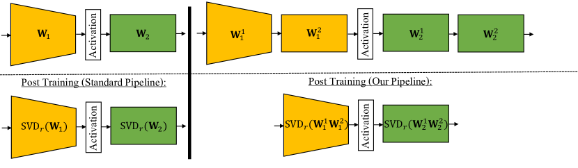
Figure 1: Illustrative example showcasing the standard (left) and our (right) pipelines. Here, a factorization of $2$ is applied to each weight matrix in a simple $2$-layered neural network. Post-training, conventional methods employ singular value truncation on the trained weights, whereas in our approach, singular value truncation is conducted on the product of two trained matrices for each weight matrix. It is important to note that, unlike [17], specifying the rank for SVT is only needed post training.

The training minimizes the objective

$$\min_{\Theta}\frac{1}{J}\sum_{i=1}^{J}\ell(\mathbf{y}(\Theta,\mathbf{x}_{i}),y_{i})+\lambda\sum_{j=1}^{N}\sum_{l=1}^{L}\|\mathbf{W}_{l}^{j}\|_{F}^{2}\>,$$

where $\lambda$ is the weight decay parameter, and $J$ is the number of data points in the training set. We note that the proposed factorization works for $m\geq n$ and $m\leq n$.

Throughout the training process, we optimize the weight matrices $\mathbf{W}^{k}_{i}$, for all $i\in[L]$, and $k\in[N]$. Following the training phase, SVD $r$-truncation is applied to each product $\mathbf{W}_{i}:=\prod_{k\in[N]}\mathbf{W}^{k}_{i}$. This involves decomposing the weight matrix into two low-rank factors, and only these factors are retained for storage. The underlying concept is that a model trained in this manner exhibits enhanced compressibility compared to the original model described by (1). The resulting weight matrices $\mathbf{W}_{i}$ demonstrate a faster decay in singular values. This strategic approach to training and approximation aims to achieve a more compact and efficient representation of the neural network trained weights, and preserve structure during inference. The procedure is outlined in Algorithm 1. Figure 1 presents an example of our proposed method.

The matrices that correspond to the weights of attention layers in (3) are treated in a similar fashion as fully-connected layers.

For convolutional layers, the fourth-order tensor $\mathbf{K}$, with dimensions $F_{H}\times F_{W}\times F_{D}\times M$, is reshaped into a matrix. This is achieved through a mode-4 unfolding, resulting in a matrix $\mathbf{K}^{(4)}$ of size $F_{H}F_{W}F_{D}\times M$. $\mathbf{K}^{(4)}$ is then expressed as a composite of $N$ matrices, denoted as $\mathbf{K}^{(4)}=\mathbf{K}^{1}\mathbf{K}^{2}\cdots\mathbf{K}^{N}$. Throughout the training phase, each $\mathbf{K}^{i}$ is updated as a weight matrix. Post-training, SVD with $r$-truncation is applied to $\mathbf{K}^{(4)}=\mathbf{K}^{1}\mathbf{K}^{2}\cdots\mathbf{K}^{N}$ to obtain low-rank factors $\mathbf{L}$ and $\mathbf{R}$, each with $r$ columns, ensuring that $\mathbf{K}^{(4)}\approx\mathbf{L}\mathbf{R}^{\top}$. During the inference phase, we first compute the convolutions of the input with the filters in $\mathbf{L}$ reshaped back to tensors, then apply $\mathbf{R}^{\top}$ to the output of the convolutions. More specifically, we reshape $\mathbf{L}$ back to a fourth-order tensor of size $F_{H}\times F_{W}\times F_{D}\times r$, denoted by $\tilde{\mathbf{L}}$, then we conduct its convolution with the input

$$\tilde{\mathbf{O}}(x,y,m^{\prime})=\sum_{i=0}^{F_{H}-1}\sum_{j=0}^{F_{W}-1}\sum_{k=0}^{F_{D}-1}\mathbf{I}(x+i,y+j,k)\mathbf{\tilde{L}}(i,j,k,m^{\prime})$$

with $m^{\prime}\in[r]$. The final output is obtained as

$$\mathbf{O}(x,y,m)=\sum_{m^{\prime}=1}^{r}\tilde{\mathbf{O}}(x,y,m^{\prime})\mathbf{R}(m,m^{\prime})\>.$$

Compared to the convolution in (2), the computational cost for a single convolution operation is reduced from $\mathcal{O}(F_{H}F_{W}F_{D}M)$ to $\mathcal{O}(F_{H}F_{W}F_{D}r)$. Similarly, the storage requirements are also decreased by a comparable magnitude.

Algorithm 1 Network Compression Via Low-Rank Promoted Training Through Linear Layers Composition.

Input: $L$ trainable weights $\mathbf{W}_{i},\forall i\in[L]$, factorization parameter $N>1$, & singular value truncation parameters $r$.
Output: Compressed and trained Weights.
1: For each $i\in[L]$
2:    Replace $\mathbf{W}_{i}$ by $\mathbf{W}^{1}_{i},\dots,\mathbf{W}^{N}_{i}$
3: Train $\mathbf{W}^{k}_{i},\forall i\in[L],\forall k\in[N]$ using Adam and weight decay.
4: For each $i\in[L]$
5:    Use $\textrm{SVD}_{r}(\prod_{k\in[N]}\mathbf{W}^{k}_{i})$ instead of $\mathbf{W}_{i}$

Next, We will explain the rationale behind our proposed approach.

4.2 Theoretical Underpinnings of LoRITa

In this subsection, we start by stating the following proposition.

Proposition 4.1.

Let $\mathbf{A}\in\mathbb{R}^{m\times n}$ be an arbitrary matrix and $r\leq\min\{m,n\}$ be its rank. For a fixed integer $M\in\mathbb{Z}_{+}$, $\mathbf{A}$ can be expressed as the product of $M$ matrices $\mathbf{R}_{i}\in\mathbb{R}^{m_{i}\times n_{i}}$ i.e., $\mathbf{A}=\prod_{i\in[M]}\mathbf{R}_{i}$ ($m_{i+1}=n_{i}\geq r$, $i=1,...,M-1$, $m_{1}=m$, $n_{M}=n$), in infinitely many ways. For any $p\in(0,1]$ and $p_{i}>0$, $\forall i\in[M]$, satisfying $\sum_{i\in[M]}\frac{1}{p_{i}}=\frac{1}{p}$, it holds

$$\begin{gathered}\|\mathbf{A}\|_{p}=\min_{\mathbf{R}_{i},i\in[M]}\Big{(}p\sum_{i\in[M]}\|\mathbf{R}_{i}\|^{p_{i}}_{p_{i}}/p_{i}\Big{)}^{1/p}\\ \textrm{s.t.}\prod_{i\in[M]}\mathbf{R}_{i}=\mathbf{A}\>.\end{gathered}$$ (6)

Proposition 4.1 closely aligns with Theorems 4 and 5 from Shang et al. [31], featuring a similar proof structure. The key distinction lies in our case’s deviation from assuming prior knowledge of the rank of $\mathbf{A}$, which is conventionally set to $\min(m,n)$.

Proposition 4.1 indicates that the Schatten-$p$ norm of any matrix is equivalent to the minimization of the weighted sum of Schatten-$p_{i}$ norm of each factor matrix by which the weights of these terms are $\frac{p}{p_{i}}$ for all $i\in[M]$.

For $p=1$, $M=2$, and $p_{1}=p_{2}=2$, (6) reduces to

$$\begin{gathered}\|\mathbf{A}\|_{*}=\min_{\mathbf{R}_{1},\mathbf{R}_{2}}\frac{1}{2}\big{(}\|\mathbf{R}_{1}\|^{2}_{F}+\|\mathbf{R}_{2}\|^{2}_{F}\big{)}\quad\\ \textrm{s.t.}\ \ \mathbf{R}_{1}\mathbf{R}_{2}=\mathbf{A}\>.\end{gathered}$$ (7)

For some integer $q>1$, let $p=\frac{1}{q}$, $M=2q$, and $p_{1}=p_{2}=\dots=p_{2q}=2$. Then, (6) becomes:

$$\begin{gathered}\|\mathbf{A}\|_{1/q}=\min_{\mathbf{R}_{i},i\in[2q]}\Big{(}\frac{1}{2q}\sum_{i\in[2q]}\|\mathbf{R}_{i}\|^{2}_{F}\Big{)}^{q}\quad\\ \textrm{s.t.}\ \ \prod_{i\in[2q]}\mathbf{R}_{i}=\mathbf{A}\>.\end{gathered}$$ (8)

If $p\in(0,1]$, minimizing the Schatten $p$-norm encourages low-rankness. A smaller $p$ strengthens the promotion of sparsity by the Schatten $p$-norm [27]. Think of the $\mathbf{A}$ matrix in (7) and (8) as weight matrices in FCNs, matricized convolutional layers in CNNs, or matrices representing query, key, and value in attention layers. These identities ((7) and (8)) imply that by re-parameterizing the weight matrix $\mathbf{A}$ as a product of $2q$ other matrices $\mathbf{R}_{i}$, where $i\in[2q]$, and using $\mathbf{R}_{i}$ (instead of $\mathbf{A}$) as the variable in gradient descent (or Adam), the weight decay on the new variable corresponds to the right-hand side of (8). Additionally, (8) suggests that the more $\mathbf{R}_{i}$ we use to represent $\mathbf{A}$, the lower rank we obtain for $\mathbf{A}$. This explains why our proposed model in (5) can achieve a lower rank for the weights compared to the traditional formulation in (1).

Remark 4.2.

While theoretically, increasing $N$ suggests an enhancement in the low-rankness of the appended trained weights, in practice, this leads to prolonged training durations. However, prioritizing shorter test times for large models is particularly crucial. This consideration is significant, especially given that testing or inference happens continuously, unlike training, which occurs only once or infrequently. This aspect significantly affects user experience, especially on resource-limited devices where compressed models are often deployed.

Remark 4.3.

In contrast to previous works, Proposition 4.1, the foundation of LoRITa, reveals that we do not assume that the weights are strictly low-rank nor require the knowledge of the weight matrix’s (approximate) rank during the training phase. Consequently, our approach encourages low-rankness without compromising the network’s capacity.

Ideally, to enforce low-rankness of the weights $W_{l}$, $l=1,...,L$, one would add the Schatten $p$ norm ($0<p<1$) penalty on each individual weight to the objective function

$$\min_{\overline{\Theta}}\frac{1}{J}\sum_{i=1}^{J}\ell(\mathbf{y}(\overline{\Theta},\mathbf{x}_{i}),y_{i})+\sum_{l=1}^{L}\alpha_{l}\|\mathbf{W}_{l}\|_{p}^{p}\>,$$

where $\overline{\Theta}=\{\mathbf{W}_{l},l=1,...,L\}$, and $\alpha_{i}>0$ are the strengths of the penalties. Proposition 4.1 indicates that if we choose $p=\frac{1}{K}$ with some even integer $K$, then we can re-parametrize the network using depth-$K$ linear factorizations and turn the above optimization into the following equivalent form that avoids the computation of SVD on-the-fly

$$\min_{\Theta}\frac{1}{J}\sum_{i=1}^{J}\ell(\mathbf{y}(\Theta,\mathbf{x}_{i}),y_{i})+\sum_{l=1}^{L}\frac{\alpha_{l}p}{2}\sum_{i=1}^{K}\|\mathbf{W}^{i}_{l}\|_{F}^{2}\>,$$ (9)

where $\Theta=\{\mathbf{W}_{l}^{i},l=1,...,L,i=1,...,K\}$.

However, (9) still has too many turning parameters $\alpha_{l}$, $i=1,...,L$. Next, we show that with ReLU activation, we can reduce the number of hyperparameters to 1.

Proposition 4.4.

With ReLU activation, the optimization problem (9) with an arbitrary choice of hyperparameters $\{\alpha_{i}\}_{i=1}^{K}$ has an equivalent single-hyper-parameter formulation

$$\min_{\Theta}\frac{1}{J}\sum_{i=1}^{J}\ell(\mathbf{y}(\Theta,\mathbf{x}_{i}),y_{i})+\lambda\sum_{l=1}^{L}\sum_{i=1}^{K}\|\mathbf{W}^{i}_{l}\|_{F}^{2}\>,$$ (10)

in the sense that they share the same networks as the minimizers.

Remark 4.5.

The proposition supports the practice of using a single weight decay parameter during network training, as is commonly done in the literature.

Proof.

The proposition is derived from the scaling ambiguity inherent in the ReLU activation. This property allows for the output of the network to remain unchanged when a scalar is multiplied by the weight matrix of one layer and the same scalar is divided by the weight matrix of another layer.

Let $\{\hat{W}^{i}_{l}$, $i\in[K],l\in[L]\}$, be the minimizer of (9). Then we can take $\lambda=\frac{p}{2}\left(\prod\limits_{i=1}^{L}\alpha_{l}\right)^{1/L}$, and verify that the rescaled weights $\{\beta_{l}\hat{W}^{i}_{l},i\in[K],l\in[L\}$ with $\beta_{l}=\sqrt{\frac{\alpha_{l}p}{2\lambda}}$ becomes the minimizer of (10). Indeed, since $\prod_{l=1}^{L}\beta_{l}=1$ (due to the definition of $\beta_{l}$ and $\lambda$), the network constructed with rescaled weights $\beta_{l}\hat{W}^{i}_{l}$ functions identically to one using the original weights $\hat{W}^{i}_{l}$. Consequently, when we insert the original and rescaled weights to (9) and (10), respectively, the first terms of the objectives are identical. Additionally, with the chosen value of $\lambda$, direct calculations confirm that the second terms in these objectives are also the same. This indicates that rescaling by $\beta_{l}$ maintains the consistency of the objective values. Now we show $\{\beta_{l}\hat{W}^{i}_{l},i\in[K],l\in[L\}$ is a (minimizer may not be unique) minimizer of (10), by contradiction. If it is not one of the minimizers, then there must exist another set of weights $\{\tilde{W}^{i}_{l},i\in[K],l\in[L\}$ that achieve lower objective values for (10). This in turn implies the reversely rescaled weights $\{\frac{1}{\beta}\tilde{W}^{i}_{l},i\in[K],l\in[L\}$ by $\beta_{l}$ must achieve the same low value for the original objective function (9). This contradicts the assumption that $\{\hat{W}^{i}_{l}$, $i\in[K],l\in[L]\}$ is a minimizer of (9). ∎

Remark 4.6.

The benefit of overparametrization in network training has been observed previously in [15, 1, 4, 13] for various reasons. Arora et al. [1] proved that overparametrization can accelerate the convergence of gradient descent in deep linear networks by analyzing the trajectory of gradient flow. Guo et al. [4] found that combining overparametrization with width expansion can enhance the overall performance of compact networks. Huh et al. [13] noted through experiments that overparametrization slightly improves the performance of the trained network, and deeper networks appear to have better rank regularization. These previous works focus on performance and acceleration. Our work complements these findings, providing numerical and theoretical evidence to justify the benefits of overparametrized weight factorization in network compression due to the weight decay behaving as a rank regularizer.

Model	Dataset	$N=1$	$N=2$	$N=3$
FCN-6	MNIST	0.983	0.982	0.977
FCN-8	MNIST	0.983	0.982	0.977
FCN-10	MNIST	0.983	0.981	0.977
ViT-L8-H1	CIFAR10	0.717	0.729	0.727
ViT-L8-H4	CIFAR10	0.710	0.718	0.701
ViT-L8-H8	CIFAR10	0.705	0.719	0.714

Table 1: Test Accuracy results of the standard ($N=1$) and our over-parameterized ($N>1$) models. The models here are trained without data augmentation.

Model	Dataset	$N=1$	$N=2$
CNN - VGG13	CIFAR10	0.919	0.922
CNN - ResNet18	CIFAR10	0.928	0.927
CNN - VGG13	CIFAR100	0.678	0.686
CNN - ResNet18	CIFAR100	0.708	0.714
ViT-L4-H8	CIFAR10	0.861	0.852
ViT-L8-H8	CIFAR10	0.865	0.857
ViT-L16-H8	CIFAR10	0.856	0.867

Table 2: Test Accuracy results of the standard ($N=1$) and our over-parameterized ($N>1$) models. The models here are trained with data augmentation.

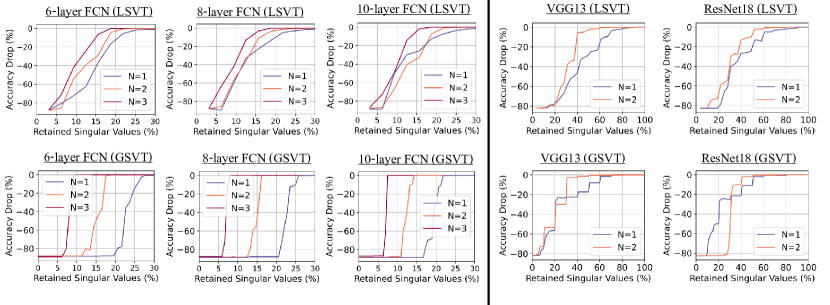
Figure 2: Low-rank compression results of FCNs on MNIST (left), and CNNs on CIFAR10 (right). The results of the top (resp. bottom) row correspond to applying the Local (resp. Global) SVT. $N=1$ results represent the baseline, whereas $N>1$ results are for the LoRITa-trained models.

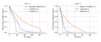
Figure 3: Empirically showing the faster decay of singular values of the first two weight matrices (layer 0 (left) and layer 1 (right)) of the standard model ($N=1$) vs. LoRITa-trained models ($N=2$ and $N=3$) using the FCN8 architecture of Table 1.

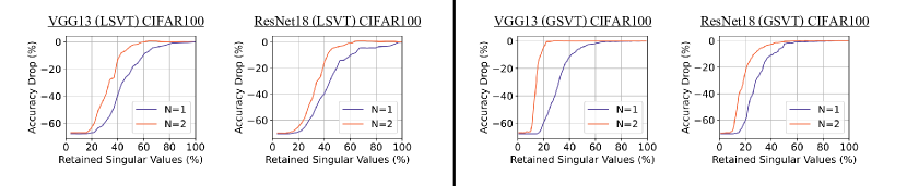
Figure 4: Low-rank compression results of the considered CNNs with applying local (left) and global (right) SVT. Here, $N=1$ (resp. $N=2$) corresponds to the models trained without (resp. with) LoRITa.

Figure 5: Low-rank compression results of the 8-layer ViT models with varied attention heads (as indicated on top of each plot) for CIFAR10. The models here are trained without data augmentation. $N=1$ denotes the baseline, while $N=2$ and $N=3$ represent our method.

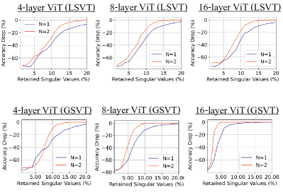
Figure 6: Low-rank compression of ViT models with data augmentation and CIFAR10 dataset. The (top) three plots correspond to applying LSVT. The (bottom) three plots correspond to applying GSVT.

5 EXPERIMENTAL RESULTS

5.1 LoRITa Evaluation on FCNs, CNNs, & ViTs

To rigorously evaluate the effectiveness of our proposed LoRITa method in achieving a rank reduction, we begin by applying this technique to FCNs. Subsequently, we expand our testing to include CNNs. Finally, we consider ViTs, motivated by the composition of their attention layers, which are essentially built from fully connected layers. The evaluation criterion is the reduction in accuracy with respect to (w.r.t.) the percentage of Retained Singular Values. The latter is defined as the number of retained singular values divided by the total number of singular values per matrix, averaged across all trained matrices. As a result, the drop in accuracy is computed by subtracting the testing accuracy with singular value truncation (SVT) from the testing accuracy without applying SVT.

A variety of models, datasets, and overparameterization scenarios are considered, as outlined in Table 1 and Table 2. For the ViT models, the number following L and H represent the number of layers and the number of heads, respectively. For comparison with baselines, we consider the models with $N=1$ (models without overparameterization using LoRITa during training). Further experimental setup details can be found in the respective captions of these tables. We use PyTorch to conduct our experiments, and our code will be released at a later date.

In each experiment, our initial phase consists of training the baseline model with optimal weight decay settings to achieve the highest achievable test accuracy. Subsequently, we apply the LoRITa method to re-parameterize the original model. This process involves initializing from a random state and fine-tuning the weight decay to ensure that the final test accuracies remain comparable to those of the initial models. See the test accuracies in Table 1 and Table 2.

Subsequently, we implement SVT on the weight matrices to compress the model, examining the impact on test accuracy as smaller singular values are eliminated. We delve into the LSVT and GSVT strategies, as discussed in Section 4, to determine which singular values to eliminate.

When employing GSVT on ViTs, singular values within the attention and fully connected layers are independently managed. Similarly, for CNNs, compression is applied distinctly to both the convolutional and fully connected layers, treating each type separately.

Evaluation on FCNs: Here, we evaluate our proposed method on fully connected neural networks, varying the number of layers, utilizing the Adam optimizer with a learning rate set to $1\times 10^{-2}$, and employing a consistent layer dimension of $96$. Overparameterization is applied across all layers in the model. To ensure a fair comparison, we begin by fine-tuning the baseline model $(N=1)$ across a range of weight decay parameters $\{5\times 10^{-6},1\times 10^{-5},2\times 10^{-4},5\times 10^{-5},1\times 10^{-4},2\times 10^{-4}\}$. Subsequently, we extend our exploration of weight decay within the same parameter range for models with $N>1$. As depicted in Table 1, setting $N$ to values larger than one results in closely matched final test accuracies. The results for FCNs on the MNIST dataset are illustrated in Figure 2(left). In these plots, LSVT (resp. GSVT) is employed for the top (resp. bottom) three plots, providing insights into the effectiveness of the proposed technique. As observed, in almost all the considered cases, models trained with $N>1$ achieve better compression results (w.r.t. the drop in test accuracy) when compared to the $N=1$ models. For the example of the 10-layer FCN model (with GSVT), using LoRITa with $N=3$ achieves no drop in test accuracy by keeping only 15% of the singular values. When LoRITa is not employed ($N=1$), the model is required to retain approximately 22% of the singular values in order to achieve the zero drop in test accuracy. It is important to highlight that the strength of the parameter $\lambda$ associated with the sparsity-promoting regularizer (in this instance, weight decay) is not selected to maximize the compression rate. Instead, the choice of $\lambda$ is geared towards maximizing the test performance of the network, as is conventionally done. Remarkably, adopting this approach still yields a commendable compression rate.

In Figure 3, we empirically demonstrate the faster decay of singular values in LoRITa-trained models. In particular, Figure 3 (left) (resp. Figure 3 (right)) show the singular values of the first (resp. second) weight matrices of the standard model ($N=1$) and LoRITa-trained models ($N=2$ and $N=3$) for the FCN8 architecture of Table 1. As observed, models trained with LoRITa exhibit faster decay, and increasing $N$ promotes faster decay.

Method	Acc.(%) ($\uparrow$)	Pruned Acc.(%) ($\uparrow$)	Pruned FLOPs(M) ($\downarrow$)	FLOPs Drop(%) ($\uparrow$)	Pruned Model Param.(M) ($\downarrow$)	Param. Drop(%) ($\uparrow$)
LoRITa ($N=3$)	91.63	91	18.47	54.7	0.11	61
LoRITa ($N=2$)	92.33	91.64	19.09	53.22	0.12	55.8
SOKS [24]	92.05	90.78	15.49	62.04	0.14	48.14
SCOP [35]	92.22	90.75	18.08	55.7	0.12	56.3
Hinge [19]	92.54	91.84	18.57	54.5	0.12	55.45
GCNP [14]	92.25	91.58	20.18	50.54	0.17	38.51
ABP [36]	92.15	91.03	21.34	0.15	45.1	95

Table 3: Evaluation of LoRITa models as compared to SOTA structured pruning/compression methods using ResNet20 on CIFAR10. The results of the other methods are reported according to Table 3 in [8] (most recent survey paper) and ranked according to the FLOPs drop percentage. The ResNet20 FLOPs (resp. parameters) is 40.81M (resp. 0.27M).

Method	Acc.(%) ($\uparrow$)	Pruned Acc.(%) ($\uparrow$)	Pruned FLOPs(M) ($\downarrow$)	FLOPs Drop(%) ($\uparrow$)	Pruned Model Param.(M) ($\downarrow$)	Param. Drop(%) ($\uparrow$)
LoRITa ($N=3$)	93.62	93.07	47.73	84.8	0.79	94.6
LoRITa ($N=2$)	94.13	93.23	50.21	84.03	0.94	93.64
EDP [29]	93.6	93.52	62.57	80.11	0.56	95.59
CHIP [32]	93.96	93.18	67.32	78.6	1.87	87.3
DLRFC [10]	93.25	93.64	72.51	76.95	0.83	94.38
EPruner [21]	93.02	93.08	74.42	76.34	1.65	88.8
CLR-RNF [22]	93.02	93.32	81.48	74.1	0.74	95

Table 4: Evaluation of LoRITa models as compared to SOTA structured pruning/compression methods using VGG16 on CIFAR10. The results of the other methods are reported according to Table 3 in [8] (most recent survey paper) and ranked according to the FLOPs drop percentage. The VGG16 FLOPs (resp. parameters) is 314.59M (resp. 14.73M).

Evaluation on CNNs: In this subsection, we evaluate the performance of our proposed method on the well-known VGG13 and ResNet18 architectures using the CIFAR10 and CIFAR100 datasets. The learning rate applied in this evaluation is set to $3\times 10^{-4}$. The weight decay was searched over $\{1\times 10^{-2},5\times 10^{-3},1\times 10^{-3}\}$ for CIFAR10 and $\{1\times 10^{-5},5\times 10^{-5},1\times 10^{-4}\}$ for CIFAR100. The results for the CIFAR10 dataset are depicted in Figure 2(right). Additionally, Figure 4 illustrates the outcomes for the CIFAR100 dataset, where the first (resp. last) two plots correspond to applying local (resp. global) SVT. Consistent with the FCN results, we observe improved compression outcomes for models trained with LoRITa. The findings from the CNN results suggest that, despite using a straightforward matricization of the convolutional filter, enhanced compression results are still evident. For the instance of VGG13, GSVT, and CIFAR100 (second plot in Figure 4), retaining 20% of the singular values, not using LoRITa results in 60% drop in accuracy, whereas our LoRITa-trained model only results in nearly 5% drop in test accuracy. Furthermore, we observe that the test accuracy of the compressed model when LoRITa is applied is slightly higher than the test accuracy of the uncompressed model. This is reported at approximately 65% retained singular values when $N=2$ in Figure 4(left).

Evaluation on ViTs: To validate the efficacy of our compression technique, we evaluate it using ViTs [2], which are noted for their capability to deliver leading-edge image classification outcomes with adequate pre-training. To comprehensively show that our training approach can yield a model of lower rank under various conditions, we first test our method on the CIFAR10 image classification task without data augmentation, employing ViTs with different head counts. Following this, we evaluate our approach on larger ViTs, incorporating data augmentation.

All the considered ViT models underwent optimization via the Adam optimizer with a learning rate of $3\times 10^{-4}$. The hidden dimension is $256$ for all ViTs. To facilitate compression, we apply overparameterization across all attention modules within the model. For a fair comparison, we initially fine-tuned the baseline model $(N=1)$ across the following weight decay parameters $\{5\times 10^{-5},1\times 10^{-4},2\times 10^{-4},5\times 10^{-4},1\times 10^{-3},2\times 10^{-3}\}$. Subsequently, we explore weight decay within the same range for our models. As evidenced in Table 1 and Table 2, setting $N$ to different values resultes in closely matched final test accuracies.

The compression effects on ViT models without data augmentation are depicted in Figure 5. We note that with a higher $N$ value, it is possible to achieve a lower model rank. The baseline model’s test accuracy begins to decline at an 85% compression rate (retaining 15% of the singular values), whereas the case of $N=3$ leads to stable test accuracy even at a 95% compression rate (retaining 5% of the singular values). We extend our evaluation to include ViTs with different layers and data augmentation (the results of Figure 6). The use of data augmentation displayed a considerable improvement in testing accuracy (before compression) as shown when comparing the ViT results of Table 1 and Table 2. Nevertheless, employing our method consistently resulted in models of a lower rank, as illustrated in Figure 5 and Figure 6.

The outcomes consistently indicate that our training approach results in models with a lower rank compared to employing only weight decay, across a variety of training configurations and network architectures.

5.2 Comparison With Structured Pruning on CNNs

In this subsection, we compare our LoRITa compression method with the structured pruning techniques delineated in Section 2. The metrics employed for this comparison are the required FLOPs and the number of parameters dropped after compression/pruning, computed using the ‘ptflops’ Python package.

The outcomes are showcased in Table 3 for the ResNet20 architecture and Table 4 for the VGG-16 architecture, both trained on the CIFAR10 dataset. The columns denote: 1) Test accuracy before pruning (%); 2) Test accuracy after pruning/compression (%); 3) FLOPs after pruning/compression (M); 4) FLOPs drop (%); 5) Pruned model parameters (M); 6) Parameters drop (%). The results of baselines are as reported in Table 3 and Table 5 of [8] for ResNet20 and VGG-16, respectively, with arrows indicating preferable results.

It’s important to underscore that the reported results in these tables are ranked based on the best achievable FLOPs drop percentage, as reducing FLOPs is the most desirable outcome when compressing and/or pruning NNs. We select the best baselines with respect to FLOPs and parameter drop, hence the different sets of methods for each architecture.

Furthermore, it’s noteworthy that following all the considered baselines, the reported results for LoRITa in Tables 3 and 4 are post one batch of fine-tuning. While most considered baselines employ multiple iterations of fine-tuning.

As long as the top-1 accuracy isn’t compromised by much (approximately 2%, as per [8]), larger FLOPs drop signifies better compression methods. It’s also imperative to note that the last column, Parameters Drop, is vital as it signifies the amount of memory reduction.

For VGG16, our result boasts the best FLOPs drop and demonstrates competitive Parameters Drop.

In the case of ResNet20, our result achieves nearly the best Parameters Drop. Although our FLOPs Drop is 8% lower than SOKS, and comparable to SCOP and Hinge. However, among these three, SCOP and Hinge underperform on VGG-16, with a FLOPs Drop of 54% and 39% (see Table 5 in [8]) respectively, in contrast to our 84%. It’s worth noting that SCOP didn’t report results for any VGG-16 networks.

We also observe that for both cases, our $N=3$ model outperforms our $N=2$ model in terms of both FLOPs Drop and Parameters Drop.

6 Conclusion

In this study, we introduced a novel approach, Low-Rank Induced Training (LoRITa). This theoretically-justified method promotes low-rankness through the composition of linear layers and achieves compression by employing singular value truncation. Notably, LoRITa accomplishes this without necessitating changes to the model structure at inference time, and it avoids the need for constrained or additional optimization steps. Furthermore, LoRITa eliminates the requirement to initialize with full-rank pre-trained models or specify rank selection before training. Our experimental validation, conducted on a diverse range of architectures and datasets, attests to the effectiveness of the proposed approach. Through rigorous testing, we have demonstrated that LoRITa yields compelling results in terms of model compression and resource efficiency, offering a promising avenue for addressing the challenges associated with deploying deep neural networks on resource-constrained platforms.

References

- Arora et al. [2018] Sanjeev Arora, Nadav Cohen, and Elad Hazan. On the optimization of deep networks: Implicit acceleration by overparameterization. In International Conference on Machine Learning, pages 244–253. PMLR, 2018.
- Beyer et al. [2022] Lucas Beyer, Xiaohua Zhai, and Alexander Kolesnikov. Better plain vit baselines for imagenet-1k. arXiv preprint arXiv:2205.01580, 2022.
- Denil et al. [2013] Misha Denil, Babak Shakibi, Laurent Dinh, Marc’Aurelio Ranzato, and Nando De Freitas. Predicting parameters in deep learning. Advances in neural information processing systems, 26, 2013.
- Guo et al. [2020] Shuxuan Guo, Jose M Alvarez, and Mathieu Salzmann. Expandnets: Linear over-parameterization to train compact convolutional networks. Advances in Neural Information Processing Systems, 33:1298–1310, 2020.
- Gural et al. [2020] Albert Gural, Phillip Nadeau, Mehul Tikekar, and Boris Murmann. Low-rank training of deep neural networks for emerging memory technology. arXiv preprint arXiv:2009.03887, 2020.
- Han et al. [2022] Kai Han, Yunhe Wang, Hanting Chen, Xinghao Chen, Jianyuan Guo, Zhenhua Liu, Yehui Tang, An Xiao, Chunjing Xu, Yixing Xu, et al. A survey on vision transformer. IEEE transactions on pattern analysis and machine intelligence, 45(1):87–110, 2022.
- Hawkins et al. [2022] Cole Hawkins, Xing Liu, and Zheng Zhang. Towards compact neural networks via end-to-end training: A bayesian tensor approach with automatic rank determination. SIAM Journal on Mathematics of Data Science, 4(1):46–71, 2022.
- He and Xiao [2023] Yang He and Lingao Xiao. Structured pruning for deep convolutional neural networks: A survey. IEEE Transactions on Pattern Analysis and Machine Intelligence, 2023.
- He et al. [2019] Yang He, Ping Liu, Ziwei Wang, Zhilan Hu, and Yi Yang. Filter pruning via geometric median for deep convolutional neural networks acceleration. In Proceedings of the IEEE/CVF conference on computer vision and pattern recognition, pages 4340–4349, 2019.
- He et al. [2022] Zhiqiang He, Yaguan Qian, Yuqi Wang, Bin Wang, Xiaohui Guan, Zhaoquan Gu, Xiang Ling, Shaoning Zeng, Haijiang Wang, and Wujie Zhou. Filter pruning via feature discrimination in deep neural networks. In European Conference on Computer Vision, pages 245–261. Springer, 2022.
- Hinton et al. [2015] Geoffrey Hinton, Oriol Vinyals, and Jeff Dean. Distilling the knowledge in a neural network. arXiv preprint arXiv:1503.02531, 2015.
- Hu et al. [2021] Edward J Hu, Yelong Shen, Phillip Wallis, Zeyuan Allen-Zhu, Yuanzhi Li, Shean Wang, Lu Wang, and Weizhu Chen. Lora: Low-rank adaptation of large language models. arXiv preprint arXiv:2106.09685, 2021.
- Huh et al. [2021] Minyoung Huh, Hossein Mobahi, Richard Zhang, Brian Cheung, Pulkit Agrawal, and Phillip Isola. The low-rank simplicity bias in deep networks. arXiv preprint arXiv:2103.10427, 2021.
- Jiang et al. [2022] Di Jiang, Yuan Cao, and Qiang Yang. On the channel pruning using graph convolution network for convolutional neural network acceleration. In IJCAI, pages 3107–3113, 2022.
- Khodak et al. [2021] Mikhail Khodak, Neil Tenenholtz, Lester Mackey, and Nicolo Fusi. Initialization and regularization of factorized neural layers. arXiv preprint arXiv:2105.01029, 2021.
- Krishnamoorthi [2018] Raghuraman Krishnamoorthi. Quantizing deep convolutional networks for efficient inference: A whitepaper. arXiv preprint arXiv:1806.08342, 2018.
- Kwon et al. [2023] Soo Min Kwon, Zekai Zhang, Dogyoon Song, Laura Balzano, and Qing Qu. Efficient compression of overparameterized deep models through low-dimensional learning dynamics. arXiv preprint arXiv:2311.05061, 2023.
- LeCun et al. [1998] Yann LeCun, Léon Bottou, Yoshua Bengio, and Patrick Haffner. Gradient-based learning applied to document recognition. Proceedings of the IEEE, 86(11):2278–2324, 1998.
- Li et al. [2020] Yawei Li, Shuhang Gu, Christoph Mayer, Luc Van Gool, and Radu Timofte. Group sparsity: The hinge between filter pruning and decomposition for network compression. In Proceedings of the IEEE/CVF conference on computer vision and pattern recognition, pages 8018–8027, 2020.
- Li et al. [2023] Zhuo Li, Hengyi Li, and Lin Meng. Model compression for deep neural networks: A survey. Computers, 12(3):60, 2023.
- Lin et al. [2021] Mingbao Lin, Rongrong Ji, Shaojie Li, Yan Wang, Yongjian Wu, Feiyue Huang, and Qixiang Ye. Network pruning using adaptive exemplar filters. IEEE Transactions on Neural Networks and Learning Systems, 33(12):7357–7366, 2021.
- Lin et al. [2022] Mingbao Lin, Liujuan Cao, Yuxin Zhang, Ling Shao, Chia-Wen Lin, and Rongrong Ji. Pruning networks with cross-layer ranking & k-reciprocal nearest filters. IEEE Transactions on neural networks and learning systems, 2022.
- Lin et al. [2018] Shaohui Lin, Rongrong Ji, Chao Chen, Dacheng Tao, and Jiebo Luo. Holistic cnn compression via low-rank decomposition with knowledge transfer. IEEE transactions on pattern analysis and machine intelligence, 41(12):2889–2905, 2018.
- Liu et al. [2022] Guangzhe Liu, Ke Zhang, and Meibo Lv. Soks: Automatic searching of the optimal kernel shapes for stripe-wise network pruning. IEEE Transactions on Neural Networks and Learning Systems, 2022.
- Marinó et al. [2023] Giosué Cataldo Marinó, Alessandro Petrini, Dario Malchiodi, and Marco Frasca. Deep neural networks compression: A comparative survey and choice recommendations. Neurocomputing, 520:152–170, 2023.
- Minaee et al. [2021] Shervin Minaee, Yuri Boykov, Fatih Porikli, Antonio Plaza, Nasser Kehtarnavaz, and Demetri Terzopoulos. Image segmentation using deep learning: A survey. IEEE transactions on pattern analysis and machine intelligence, 44(7):3523–3542, 2021.
- Nie et al. [2012] Feiping Nie, Heng Huang, and Chris Ding. Low-rank matrix recovery via efficient schatten p-norm minimization. In Proceedings of the AAAI Conference on Artificial Intelligence, volume 26, pages 655–661, 2012.
- Ravishankar et al. [2019] Saiprasad Ravishankar, Jong Chul Ye, and Jeffrey A Fessler. Image reconstruction: From sparsity to data-adaptive methods and machine learning. Proceedings of the IEEE, 108(1):86–109, 2019.
- Ruan et al. [2021] Xiaofeng Ruan, Yufan Liu, Chunfeng Yuan, Bing Li, Weiming Hu, Yangxi Li, and Stephen Maybank. Edp: An efficient decomposition and pruning scheme for convolutional neural network compression. IEEE Transactions on Neural Networks and Learning Systems, 32(10):4499–4513, 2021. 10.1109/TNNLS.2020.3018177.
- Rumelhart et al. [1986] D. E. Rumelhart, J. L. McClelland, and the PDP Research Group. Parallel Distributed Processing: Explorations in the Microstructure of Cognition (Vol. 2). MIT Press, 1986.
- Shang et al. [2016] Fanhua Shang, Yuanyuan Liu, and James Cheng. Unified scalable equivalent formulations for schatten quasi-norms. arXiv preprint arXiv:1606.00668, 2016.
- Sui et al. [2021] Yang Sui, Miao Yin, Yi Xie, Huy Phan, Saman Aliari Zonouz, and Bo Yuan. Chip: Channel independence-based pruning for compact neural networks. Advances in Neural Information Processing Systems, 34:24604–24616, 2021.
- Sui et al. [2024] Yang Sui, Miao Yin, Yu Gong, Jinqi Xiao, Huy Phan, and Bo Yuan. Elrt: Efficient low-rank training for compact convolutional neural networks. arXiv preprint arXiv:2401.10341, 2024.
- Tai et al. [2015] Cheng Tai, Tong Xiao, Yi Zhang, Xiaogang Wang, et al. Convolutional neural networks with low-rank regularization. arXiv preprint arXiv:1511.06067, 2015.
- Tang et al. [2020] Yehui Tang, Yunhe Wang, Yixing Xu, Dacheng Tao, Chunjing Xu, Chao Xu, and Chang Xu. Scop: Scientific control for reliable neural network pruning. Advances in Neural Information Processing Systems, 33:10936–10947, 2020.
- Tian et al. [2021] Guanzhong Tian, Yiran Sun, Yuang Liu, Xianfang Zeng, Mengmeng Wang, Yong Liu, Jiangning Zhang, and Jun Chen. Adding before pruning: Sparse filter fusion for deep convolutional neural networks via auxiliary attention. IEEE Transactions on Neural Networks and Learning Systems, 2021.
- Vaswani et al. [2017] Ashish Vaswani, Noam Shazeer, Niki Parmar, Jakob Uszkoreit, Llion Jones, Aidan N Gomez, Łukasz Kaiser, and Illia Polosukhin. Attention is all you need. Advances in neural information processing systems, 30, 2017.
- Waleffe and Rekatsinas [2020] Roger Waleffe and Theodoros Rekatsinas. Principal component networks: Parameter reduction early in training. arXiv preprint arXiv:2006.13347, 2020.
- Yang et al. [2023] Ling Yang, Zhilong Zhang, Yang Song, Shenda Hong, Runsheng Xu, Yue Zhao, Wentao Zhang, Bin Cui, and Ming-Hsuan Yang. Diffusion models: A comprehensive survey of methods and applications. ACM Computing Surveys, 56(4):1–39, 2023.
- Yu et al. [2017] Xiyu Yu, Tongliang Liu, Xinchao Wang, and Dacheng Tao. On compressing deep models by low rank and sparse decomposition. In Proceedings of the IEEE conference on computer vision and pattern recognition, pages 7370–7379, 2017.
- Zhang et al. [2018] Xiangyu Zhang, Xinyu Zhou, Mengxiao Lin, and Jian Sun. Shufflenet: An extremely efficient convolutional neural network for mobile devices. In Proceedings of the IEEE conference on computer vision and pattern recognition, pages 6848–6856, 2018.