A View on Out-of-Distribution Identification from
a Statistical Testing Theory Perspective
Abstract
We study the problem of efficiently detecting Out-of-Distribution (OOD) samples at test time in supervised and unsupervised learning contexts. While ML models are typically trained under the assumption that training and test data stem from the same distribution, this is often not the case in realistic settings, thus reliably detecting distribution shifts is crucial at deployment. We re-formulate the OOD problem under the lenses of statistical testing and then discuss conditions that render the OOD problem identifiable in statistical terms. Building on this framework, we study convergence guarantees of an OOD test based on the Wasserstein distance, and provide a simple empirical evaluation.
1 Introduction
Supervised and unsupervised learning models traditionally operate under the assumption that the distributions of data observed during training and testing are the same (Murphy, 2012). However, this ideal scenario rarely holds true in real-world applications, where data distributions can shift. OOD detection generally refers to the task of identifying instances that lie outside the distribution of data seen during training (Yang et al., 2021; Liu et al., 2021). It serves as a crucial component towards safe and trustworthy AI when deploying machine learning models in real-world scenarios such as self-driving cars (e.g., (Ji et al., 2021)), medical diagnostics and cybersecurity (Hendrycks et al., 2021). Failure to accurately detect OOD samples in these settings can lead to severe consequences.
There is a very rich literature on methods to detect OOD. Some highly influential contributions include: Hendrycks and Gimpel (2016); Liang et al. (2018); Sun et al. (2021), that propose a softmax score for neural networks; Ren et al. (2019) that advocates for likelihood ratios based scores; Liu et al. (2020) that instead utilize energy-based scores; and Huang et al. (2021) that uses gradient information of the KL divergence. Theoretical studies on the problem of OOD detection are limited. Recent works include Ye et al. (2021); Fort et al. (2021) and Morteza and Li (2022). In particular, Zhang et al. (2021) analyzes the causes of failures in OOD detection with generative models, while Fang et al. (2022) derive conditions for learnability of the OOD problem under a PAC-learnability framework.
In this work, we adopt a statistical testing approach to the problem (Lehmann et al., 1986). While this perspective is not entirely new (Zhang et al., 2021; Haroush et al., 2022), we progress a step further and derive theoretical guarantees under a non-parametric statistical testing framework based on the Wasserstein distance (Vallender, 1974; Panaretos and Zemel, 2019). These results help understand the conditions for identifiability of the OOD classification problem.
2 Problem Framework
Suppose we are in a supervised learning setting and we observe i.i.d. data at training time, stemming from the joint distribution (In-Distribution, or ID). At test time, data might generate either from the same joint distribution as training , or a fixed out-of-training (OOD) joint distribution . Thus, at test time, data points are sampled from the mixture
where indicates the prevalence of OOD samples. In this supervised learning context, a distribution shift in the joint can stem from either a shift in the marginal , also known as ‘covariate shift’, or in the marginal , known as ‘semantic shift’, or in both at the same time (Yang et al., 2021). In unsupervised settings shifts can occur only in . In typical supervised learning settings however, at test time, we do not observe output labels . Yet, this is not always the case. For example in online learning we observe a stream of independent pairs that we can use to update the model, thus we can possibly detect both anomalies in and in . Finally, in time series we observe a stream of temporally dependent data points, where the objective is to detect a change point in time (Saatçi et al., 2010; Aminikhanghahi and Cook, 2017; Van den Burg and Williams, 2020). Given these different types of data streaming, we define the generalized OOD detection problem as follows
Problem 2.1 (OOD Detection).
Given an ID distribution and training data , the aim is to construct a binary classifier such that
where denotes the -th entry of the test dataset.
The analogy between the ‘zero-shot’ OOD classification problem above and statistical tests has been drawn by recent works (Zhang et al., 2021; Haroush et al., 2022). In statistical testing theory (Lehmann et al., 1986), the goal is to test a null versus an alternative hypothesis VS , via a test indicator function , where is a random variable, is a test statistic and an acceptance region. Also, we denote the power of a test, or True Positive Rate (TPR), as the probability of accepting when this is true: ,. We can then draw the following equivalence between OOD detection and a ‘goodness-of-fit’ tests:
Remark 2.2 (OOD Test).
Given the hypotheses , Problem 2.1 is a statistical testing problem where , with test statistic and critical value .
The critical test value is usually cross-validated using the training data, and indicates the type-I error probability of the test (typical values are ). The task is to design a test statistic that gives the best guarantees in terms of test power (equivalently known as False Positive Rate).
3 A Wasserstein Distance OOD Test
The test statistic we consider is based on the Wasserstein distance. The -Wasserstein distance is defined, given two probability measures and on , as
where is the space of all couplings of and (joint probability measures whose marginals are and ). The Wasserstein distance, unlike other distributional divergences, possesses typical metric properties, such as symmetry and triangle inequality (Ramdas et al., 2017; Panaretos and Zemel, 2019), that we need in order to derive the results in the next section. The Wasserstein OOD test is sketched out as follows. A model of the data generating distribution (e.g., regression, classification, generative, etc.), parametrized by , is learnt using . Then, at test time, the test statistic for the hypotheses vs is defined as , replacing with its sample equivalent, and the critical test value is computed as the on the training data.
3.1 OOD Identifiability and Test Power
In this section we derive theoretical properties of the Wasserstein OOD test, and we use these to shed light on the identifiability, or learnability (Fang et al., 2022), of the OOD detection problem more in general. We start by demonstrating that, in the limit of OOD samples , the Wasserstein OOD test is uniformly consistent, i.e., its power (or True Positive Rate) , under some specific condition linking the ID and the OOD distributions. Let be the OOD samples at test time, a scalar depending only on , and the OOD distribution corresponding to a certain , then we have:
Theorem 3.1 (Uniform Consistency).
Let be a test dataset. The test based on for hypotheses vs , is such that
as , over alternatives that satisfy , where .
Proof is provided in the appendix. The intuition behind Thm. 3.1 is that the test power (or TPR) of is asymptotically optimal in the limit of if the OOD is far enough from the ID . Thus, the OOD detection problem is ‘identifiable’ when there is asymptotically no ‘overlap’ between the ID and OOD distributions (note that this is valid for any test) (Ye et al., 2021; Fang et al., 2022). Notice that while we prove consistency in terms of Wasserstein distance, the same result can in theory be obtained also for other distributional distances, for example Kolmogorov-Smirnov (KS) distance (but not the KL and JS divergence, which are not symmetric and do not satisfy the triangle inequality). However, as we will discuss later, Wasserstein distance also has practical implementation advantages; e.g., KS distance cannot easily be computed for multivariate distributions.
While uniform consistency holds in the limit of , we can also derive a non-asymptotic lower bound on using concentration inequalities as follows. Notice that, contrary to Thm. 3.1, the following results pertain uniquely to the Wasserstein distance case.
Theorem 3.2 (Non-Asymptotic Lower Bound).
Let be a test dataset. The test for hypotheses vs , is such that
if and .
Here, and are defined according to the appendix. What happends then if condition does not hold, i.e., when and are very near (‘near OOD’)? We can derive a worst case upper bound of the distance based tests as follows.
Theorem 3.3 (Worst Case Upper Bound).
Let be a test dataset. The test for hypotheses vs , is such that
as , for alternatives satisfying .
This means that the OOD detection problem is not identifiable for OOD distrubutions such that . In fact, no test can have high power in such cases where the OOD distribution is at a distance from (Lehmann et al., 1986). Lastly, we derive an asymptotic upper bound for the ‘intermediate’ case of not diverging nor converging to 0, but of distance converging to a constant , such as the one depicted in the MNIST example in Section 4.2. This reads:
Theorem 3.4 (Intermediate Case Asymptotic Upper Bound).
Let be a test dataset. The test for hypotheses vs , is such that
for alternatives such that .
In general, for the case where and , the test power will converge to a limit strictly between and .
3.2 Distributional Distance Tests
The theoretical results in the previous section shed light on the identifiability of the OOD detection problem, by laying out the conditions that guarantee certain upper bounds or convergence in terms of test power, or TPR, . Although these results pertain to the proposed Wasserstein distance OOD test, they can be in theory obtained also for other distributional distances (e.g., total variation distance, KS distance, etc.). In this section we explain why distributional distances are preferable, compared, e.g., to entropy and k-NN based tests (Ren et al., 2019) and detail the advantages of using Wasserstein distance specifically.
Q1: Why Distance Based OOD Tests?
OOD metrics based on distributional distances guarantee that aleatoric (pure noise) components are removed from consideration. To prove this point, consider the Shannon entropy (Shannon, 1948) of a distribution over a random variable , , as a measure of Total Variation (TV) of . TV can be decomposed w.r.t. another random variable into the following (Cover, 1999):
The conditional entropy is a natural measure of aleatoric uncertainty or pure noise, that does not bear any ‘semantic’ information (e.g., an image background). Conversely, the mutual information , where is the KL divergence (Lindley, 1956), is a measure of epistemic uncertainty only, as it represents how much information can be gained on by observing realizations of (and viceversa), net of aleatoric components. In an OOD context this means intuitively that the smaller , the more likely it is that we are observing data from the same distribution, . Finally, notice that there is a direct link between KL-divergence and Wasserstein distance (see Appendix B.1), such that both are infact different measures of mutual information .
Q2: Why Wasserstein Distance?
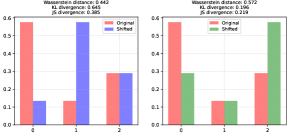
Inspired by optimal transport theory, the Wasserstein distance has clear geometric interpretations, and it embeds information about the geometry of the support (Panaretos and Zemel, 2019); see Figure 1 above for an example. Thus, compared to the popular KL and JS divergences, Wasserstein can provide meaningful and smooth representations of the distance between two distributions and , even when there is no overlap between them (Arjovsky et al., 2017); see example in Section 6.2 of Weng (2019). Theoretical results in Section 3.1 thus are not derivable for the KL divergence case, as this is not symmetric and does not satisfy the triangle inequality. Compared to KS distance (used in KS tests) instead, Wasserstein distance can be easily applied to multivariate data, whereas the former requires multivariate empirical cumulative distribution functions, which are notoriously hard to compute (Justel et al., 1997; Langrené and Warin, 2021). Then finally, contrary to parametric families of distances (e.g., Mahalanobis distance, even though this is technically a distance between a point and a distribution), it does not necessarily need parametric assumptions, although these can simplify computations as we show in the section below.
Eventually, we stress that in the case of (multivariate) Gaussian distributions, the computation of distances mentioned above can be heavily simplified to closed form operation. In Appendix B.2, we include the simplified version of KL Divergence and 2-Wasserstein Distance for the case of and being multivariate Gaussians.
4 Experiments
In this section we present results from two experiments: the first is a simple depiction of how test power changes depending on overlap, while the second implements some of the OOD tests on a image classification problem111Code is provided at https://github.com/albicaron/OOD_test..
4.1 Generative Model Example
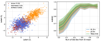
Suppose we access a high-dimensional dataset at training time consisting of continuous , where . We set and as training sample and feature dimensions. We want to learn a simple generative model for , by assuming that these are generated by lower dimensional features with where . For visualization purposes, we pick , generated randomly as a , where . We learn via a Factor Loading (FL) model (Gorsuch, 2014), where and the latent factors are unobserved and assumed to be , the noise is . At test time we assume we sequentially receive independent sample batches of size , , and we have to detect whether a batch OOD w.r.t. the training sample (this could be the case, e.g., in quality assurance/control problems, continuous authentication in security (Eberz et al., 2017) or experimental design) through their latent features .
We construct an OOD test to assess whether a test batch is OOD as follows: i) split the data into 80%-20% train-validation; ii) fit a FL model on the 80% train set and compute the estimated latent factors ; iii) use the 20% validation set to compute the estimated ; iv) Compute the KL, JS and Wasserstein distances between the FL estimated and — notice that these densities are both -dimensional Gaussians by model assumption, so we can use the computational simplifications of Appendix B.2; v) Repeat the previous steps for folds and compute the OOD test critical value as the quantile of each distance . At test time we observe a sequence of 100 independent sample batches, of which 50% are ID, while 50% are OOD and exhibit a shift in the latent features away from the ID mean, and equal to times the standard deviation of the true train ID features .
We report in Figure 5 the following quantities: the first plot on the left depicts the true latent features , the estimated features via FL, and the features subject to an OOD distributional shift; the plot on the right instead reports the Area Under the Receiver Operating Characteristic (AUROC) curve, computed between the true positive rates (test power) and the false positive rates (probability of type-I error for each method, for increasing values of OOD mean shift (in terms of number of standard deviations). Notice that AUROC reaches the optimal 95% level for all the OOD tests, as the OOD distribution more clearly separates from the ID one and overlap reduces.
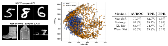
4.2 MNIST Classification
The second experiment involves an image classification task. We consider the MNIST dataset at training time, and learn a CNN probabilistic classifier on the labels in . At test time, we receive 50% of samples from MNIST (ID) and 50% samples from Fashion MNIST, which is treated as the OOD dataset, and we have to correctly detect which ones are OOD. Samples from each dataset are depicted in the first plot on the left in Figure 3. In the middle plot of Figure 3, we report the two principal latent features of each dataset, learnt via Truncated SVD. As can be seen their distributions appear to have a good degree of overlap, which is not surprising as MNIST and Fashion MNIST images share common patterns. The OOD tests are constructed similarly to Section 4.1, using the softmax distributions . We consider a standard ‘max-softmax’ OOD detector (Hendrycks and Gimpel, 2016; Liang et al., 2018), an entropy based detector (that computes the entropy of the softmax distribution, and a KL and Wasserstein distance OOD detectors. For the KL and Wasserstein detectors, the distance is computed between and the uniform distribution as a reference. Results in terms of AUROC, TPR and FPR are reported in the table on the right of Figure 3, and show that the Wasserstein based OOD test slightly outperforms the others.
5 Conclusion
In this short paper we present novel theoretical results that shed light on the identifiability of OOD detection (Fang et al., 2022). These results stem from recasting the problem as one of statistical testing and leverage the properties of the Wasserstein distance to derive asymptotic and non-asymptotic bounds on test power. We conclude with two simple experiments on generative modelling and classification.
Acknowledgments
Research funded by the Defence Science and Technology Laboratory (Dstl) which is an executive agency of the UK Ministry of Defence providing world class expertise and delivering cutting-edge science and technology for the benefit of the nation and allies. The research supports the Autonomous Resilient Cyber Defence (ARCD) project within the Dstl Cyber Defence Enhancement programme.
References
- Aminikhanghahi and Cook [2017] Samaneh Aminikhanghahi and Diane J Cook. A survey of methods for time series change point detection. Knowledge and information systems, 51(2):339–367, 2017.
- Arjovsky et al. [2017] Martin Arjovsky, Soumith Chintala, and Léon Bottou. Wasserstein generative adversarial networks. In International conference on machine learning, pages 214–223. PMLR, 2017.
- Bernardo [1979] José M Bernardo. Expected information as expected utility. the Annals of Statistics, pages 686–690, 1979.
- Bolley et al. [2007] François Bolley, Arnaud Guillin, and Cédric Villani. Quantitative concentration inequalities for empirical measures on non-compact spaces. Probability Theory and Related Fields, 137:541–593, 2007.
- Bonneel et al. [2015] Nicolas Bonneel, Julien Rabin, Gabriel Peyré, and Hanspeter Pfister. Sliced and radon wasserstein barycenters of measures. Journal of Mathematical Imaging and Vision, 51:22–45, 2015.
- Cai and Lim [2022] Yuhang Cai and Lek-Heng Lim. Distances between probability distributions of different dimensions. IEEE Transactions on Information Theory, 68(6):4020–4031, 2022.
- Cover [1999] Thomas M Cover. Elements of information theory. John Wiley & Sons, 1999.
- Daxberger and Hernández-Lobato [2019] Erik Daxberger and José Miguel Hernández-Lobato. Bayesian variational autoencoders for unsupervised out-of-distribution detection. arXiv preprint arXiv:1912.05651, 2019.
- Eberz et al. [2017] Simon Eberz, Kasper B Rasmussen, Vincent Lenders, and Ivan Martinovic. Evaluating behavioral biometrics for continuous authentication: Challenges and metrics. In Proceedings of the 2017 ACM on Asia conference on computer and communications security, pages 386–399, 2017.
- Fang et al. [2022] Zhen Fang, Yixuan Li, Jie Lu, Jiahua Dong, Bo Han, and Feng Liu. Is out-of-distribution detection learnable? Advances in Neural Information Processing Systems, 35:37199–37213, 2022.
- Fort et al. [2021] Stanislav Fort, Jie Ren, and Balaji Lakshminarayanan. Exploring the limits of out-of-distribution detection. Advances in Neural Information Processing Systems, 34:7068–7081, 2021.
- Foster [2021] Adam Evan Foster. Variational, Monte Carlo and policy-based approaches to Bayesian experimental design. PhD thesis, University of Oxford, 2021.
- Gal et al. [2017] Yarin Gal, Riashat Islam, and Zoubin Ghahramani. Deep bayesian active learning with image data. In International conference on machine learning, pages 1183–1192. PMLR, 2017.
- Ghosal and Van der Vaart [2017] Subhashis Ghosal and Aad Van der Vaart. Fundamentals of nonparametric Bayesian inference, volume 44. Cambridge University Press, 2017.
- Gorsuch [2014] Richard L Gorsuch. Factor analysis: Classic edition. Routledge, 2014.
- Hallin et al. [2021] Marc Hallin, Gilles Mordant, and Johan Segers. Multivariate goodness-of-fit tests based on wasserstein distance. Electronic Journal of Statistics, 15:1328–1371, 2021.
- Hanneke and others [2014] Steve Hanneke et al. Theory of disagreement-based active learning. Foundations and Trends® in Machine Learning, 7(2-3):131–309, 2014.
- Haroush et al. [2022] Matan Haroush, Tzviel Frostig, Ruth Heller, and Daniel Soudry. A statistical framework for efficient out of distribution detection in deep neural networks. In International Conference on Learning Representations, 2022.
- Hendrycks and Gimpel [2016] Dan Hendrycks and Kevin Gimpel. A baseline for detecting misclassified and out-of-distribution examples in neural networks. In International Conference on Learning Representations, 2016.
- Hendrycks et al. [2021] Dan Hendrycks, Nicholas Carlini, John Schulman, and Jacob Steinhardt. Unsolved problems in ml safety. arXiv preprint arXiv:2109.13916, 2021.
- Houlsby et al. [2011] Neil Houlsby, Ferenc Huszár, Zoubin Ghahramani, and Máté Lengyel. Bayesian active learning for classification and preference learning. arXiv preprint arXiv:1112.5745, 2011.
- Huang et al. [2021] Rui Huang, Andrew Geng, and Yixuan Li. On the importance of gradients for detecting distributional shifts in the wild. Advances in Neural Information Processing Systems, 34:677–689, 2021.
- Izmailov et al. [2018] Pavel Izmailov, Dmitrii Podoprikhin, Timur Garipov, Dmitry Vetrov, and Andrew Gordon Wilson. Averaging weights leads to wider optima and better generalization. In 34th Conference on Uncertainty in Artificial Intelligence 2018, pages 876–885, 2018.
- Ji et al. [2021] Xiaoyu Ji, Yushi Cheng, Yuepeng Zhang, Kai Wang, Chen Yan, Wenyuan Xu, and Kevin Fu. Poltergeist: Acoustic adversarial machine learning against cameras and computer vision. In 2021 IEEE Symposium on Security and Privacy (SP), pages 160–175. IEEE, 2021.
- Justel et al. [1997] Ana Justel, Daniel Peña, and Rubén Zamar. A multivariate kolmogorov-smirnov test of goodness of fit. Statistics & probability letters, 35(3):251–259, 1997.
- Langrené and Warin [2021] Nicolas Langrené and Xavier Warin. Fast multivariate empirical cumulative distribution function with connection to kernel density estimation. Computational Statistics & Data Analysis, 162:107267, 2021.
- Lee et al. [2018] Kimin Lee, Kibok Lee, Honglak Lee, and Jinwoo Shin. A simple unified framework for detecting out-of-distribution samples and adversarial attacks. Advances in neural information processing systems, 31, 2018.
- Lehmann et al. [1986] Erich Leo Lehmann, Joseph P Romano, and George Casella. Testing statistical hypotheses, volume 3. Springer, 1986.
- Liang et al. [2018] Shiyu Liang, Yixuan Li, and R Srikant. Enhancing the reliability of out-of-distribution image detection in neural networks. In International Conference on Learning Representations, 2018.
- Lindley [1956] Dennis V Lindley. On a measure of the information provided by an experiment. The Annals of Mathematical Statistics, 27(4):986–1005, 1956.
- Liu et al. [2020] Weitang Liu, Xiaoyun Wang, John Owens, and Yixuan Li. Energy-based out-of-distribution detection. Advances in neural information processing systems, 33:21464–21475, 2020.
- Liu et al. [2021] Jiashuo Liu, Zheyan Shen, Yue He, Xingxuan Zhang, Renzhe Xu, Han Yu, and Peng Cui. Towards out-of-distribution generalization: A survey. arXiv preprint arXiv:2108.13624, 2021.
- Ming et al. [2022] Yifei Ming, Hang Yin, and Yixuan Li. On the impact of spurious correlation for out-of-distribution detection. In Proceedings of the AAAI Conference on Artificial Intelligence, volume 36, pages 10051–10059, 2022.
- Morteza and Li [2022] Peyman Morteza and Yixuan Li. Provable guarantees for understanding out-of-distribution detection. In Proceedings of the AAAI Conference on Artificial Intelligence, volume 36, pages 7831–7840, 2022.
- Murphy [2012] Kevin P Murphy. Machine learning: a probabilistic perspective. MIT press, 2012.
- Nietert et al. [2021] Sloan Nietert, Ziv Goldfeld, and Kengo Kato. Smooth -wasserstein distance: structure, empirical approximation, and statistical applications. In International Conference on Machine Learning, pages 8172–8183. PMLR, 2021.
- Ovadia et al. [2019] Yaniv Ovadia, Emily Fertig, Jie Ren, Zachary Nado, David Sculley, Sebastian Nowozin, Joshua Dillon, Balaji Lakshminarayanan, and Jasper Snoek. Can you trust your model’s uncertainty? evaluating predictive uncertainty under dataset shift. Advances in neural information processing systems, 32, 2019.
- Panaretos and Zemel [2019] Victor M Panaretos and Yoav Zemel. Statistical aspects of wasserstein distances. Annual review of statistics and its application, 6:405–431, 2019.
- Pukelsheim [2006] Friedrich Pukelsheim. Optimal design of experiments. SIAM, 2006.
- Rahaman and others [2021] Rahul Rahaman et al. Uncertainty quantification and deep ensembles. Advances in Neural Information Processing Systems, 34:20063–20075, 2021.
- Rainforth et al. [2023] Tom Rainforth, Adam Foster, Desi R Ivanova, and Freddie Bickford Smith. Modern bayesian experimental design. arXiv preprint arXiv:2302.14545, 2023.
- Ramdas et al. [2017] Aaditya Ramdas, Nicolás García Trillos, and Marco Cuturi. On wasserstein two-sample testing and related families of nonparametric tests. Entropy, 19(2):47, 2017.
- Rasmussen et al. [2006] Carl Edward Rasmussen, Christopher KI Williams, et al. Gaussian processes for machine learning, volume 1. Springer, 2006.
- Ren et al. [2019] Jie Ren, Peter J Liu, Emily Fertig, Jasper Snoek, Ryan Poplin, Mark Depristo, Joshua Dillon, and Balaji Lakshminarayanan. Likelihood ratios for out-of-distribution detection. Advances in neural information processing systems, 32, 2019.
- Saatçi et al. [2010] Yunus Saatçi, Ryan D Turner, and Carl E Rasmussen. Gaussian process change point models. In Proceedings of the 27th International Conference on Machine Learning (ICML-10), pages 927–934, 2010.
- Shannon [1948] Claude Elwood Shannon. A mathematical theory of communication. The Bell system technical journal, 27(3):379–423, 1948.
- Sun et al. [2021] Yiyou Sun, Chuan Guo, and Yixuan Li. React: Out-of-distribution detection with rectified activations. Advances in Neural Information Processing Systems, 34:144–157, 2021.
- Sun et al. [2022] Yiyou Sun, Yifei Ming, Xiaojin Zhu, and Yixuan Li. Out-of-distribution detection with deep nearest neighbors. In International Conference on Machine Learning, pages 20827–20840. PMLR, 2022.
- Vallender [1974] SS Vallender. Calculation of the wasserstein distance between probability distributions on the line. Theory of Probability & Its Applications, 18(4):784–786, 1974.
- Van den Burg and Williams [2020] Gerrit JJ Van den Burg and Christopher KI Williams. An evaluation of change point detection algorithms. arXiv preprint arXiv:2003.06222, 2020.
- Vaswani et al. [2017] Ashish Vaswani, Noam Shazeer, Niki Parmar, Jakob Uszkoreit, Llion Jones, Aidan N Gomez, Łukasz Kaiser, and Illia Polosukhin. Attention is all you need. Advances in neural information processing systems, 30, 2017.
- Weng [2019] Lilian Weng. From gan to wgan. arXiv preprint arXiv:1904.08994, 2019.
- Wilson and Izmailov [2020] Andrew G Wilson and Pavel Izmailov. Bayesian deep learning and a probabilistic perspective of generalization. Advances in neural information processing systems, 33:4697–4708, 2020.
- Wilson [2020] Andrew Gordon Wilson. The case for bayesian deep learning. arXiv preprint arXiv:2001.10995, 2020.
- Yang et al. [2021] Jingkang Yang, Kaiyang Zhou, Yixuan Li, and Ziwei Liu. Generalized out-of-distribution detection: A survey. arXiv preprint arXiv:2110.11334, 2021.
- Ye et al. [2021] Haotian Ye, Chuanlong Xie, Tianle Cai, Ruichen Li, Zhenguo Li, and Liwei Wang. Towards a theoretical framework of out-of-distribution generalization. Advances in Neural Information Processing Systems, 34:23519–23531, 2021.
- Zhang et al. [2021] Lily Zhang, Mark Goldstein, and Rajesh Ranganath. Understanding failures in out-of-distribution detection with deep generative models. In International Conference on Machine Learning, pages 12427–12436. PMLR, 2021.
Appendix A Proofs of Theorems
In this first appendix section, we report the proofs for the theorem presented in the main body of the work. We make sure of the cleaner notation for a -Wasserstein distance.
Theorem A.1 (Restatement of Theorem 3.1).
Let be a test dataset. The test based on for hypotheses vs , is such that
as , over alternatives that satisfy , where .
Proof.
Let be a sequence of probabilities depending on satisfying . Then, letting be an estimate of , by the triangle inequality of Wasserstein distance we have:
which implies:
Due to continuity of the cumulative distribution function relative to the random variable , , we can write , which can be written as
Now, we have that is a tight sequence, i.e., with , and arbitrarily small. Thus we have that
implying at the same time, since and , so that . ∎
We proceed with the proof of non-asymptotic lower bounds of Theorem 3.2.
Theorem A.2 (Restatement of Theorem 3.2).
Let be a test dataset. The test for hypotheses vs , is such that
if and .
Proof.
Starting again from the triangle inequality property of Wasserstein distance as in the previous proof, we can obtain
Again, in the same way of the previous proof we can apply the cumulative distribution function and obtain
Now, we make use of Wasserstein Concentration inequality theorem stated in Bolley et al. [2007] that reads
Theorem A.3 (Bolley et al. [2007]).
Let and let be a probability on satisfying
For and , there exists some constant such that for we have
where:
Applying the concentration inequality result of Bolley et al. [2007] above to our can we can derive the following
∎
We proceed with the proof of Thm. 3.3 for the worst-case scenario where the two distributions tend to .
Theorem A.4 (Restatement of Theorem 3.3).
Let be a test dataset. The test for hypotheses vs , is such that
as , for alternatives satisfying .
Proof.
Starting from the Wasserstein triangle inequality:
We can apply the cumulative distribution function to get , that we can write as
And then condition trivially implies that in reality ( is true) and thus, by construction of the test, we have that: test power for accepting against alternative type-I error probability . Which translate into:
∎
Eventually, we conclude by proving Thm 3.4 for the intermediate case where , such as the one depicted in the MNIST example.
Theorem A.5 (Restatement of Theorem 3.4).
Let be a test dataset. The test for hypotheses vs , is such that
for alternatives such that .
Appendix B Additional Information on Distances
Firstly, we report here the definitions of some of the distances mentioned throughout the body of the paper. Let be a compact metric set and let be probability distributions defined on , then we can define the following distribution divergences/distances:
-
•
The Kolmogorov-Smirnov (KS) Distance:
where is the cumulative distribution function evaluated at
-
•
The Kullback-Leibler (KL) Divergence:
where and are density functions
-
•
The Jensen-Shannon (JS) Divergence:
where is a mixture probability measure
-
•
The Wasserstein (W) Distance:
where is the space of all couplings of and (joint probability measures whose marginals are and ).
B.1 Link between KL and Wasserstein Distance
In this Appendix subsection we briefly sketch the mathematical relationship between the KL divergence and the Wasserstein distance. Following results in Cai and Lim [2022] we have that:
where is the Total Variation (TV) distance . While on the other hand then we have that
Thus putting the two together:
B.2 Simplifications for Gaussian Densities
We conclude by including simplification of KL divergence and Wasserstein distance in the case of and being (multivariate) Gaussian distributions, and . For the KL divergence we have
While for the Wasserstein distance case we have: