Functional Post-Clustering Selective Inference with Applications to EHR Data Analysis

Abstract

In electronic health records (EHR) analysis, clustering patients according to patterns in their data is crucial for uncovering new subtypes of diseases. Existing medical literature often relies on classical hypothesis testing methods to test for differences in means between these clusters. Due to selection bias induced by clustering algorithms, the implementation of these classical methods on post-clustering data often leads to an inflated type-I error. In this paper, we introduce a new statistical approach that adjusts for this bias when analyzing data collected over time. Our method extends classical selective inference methods for cross-sectional data to longitudinal data. We provide theoretical guarantees for our approach with upper bounds on the selective type-I and type-II errors. We apply the method to simulated data and real-world Acute Kidney Injury (AKI) EHR datasets, thereby illustrating the advantages of our approach.

1 Introduction

Testing for a difference in means between groups of functional data is fundamental to answering research questions across various scientific areas (Fan and Lin, 1998; Cuevas et al., 2004; Zhang and Chen, 2007; Zhang, 2014). Recently, there has been an increasing demand for post-clustering inference of functional data, namely, testing the difference between groups discovered by clustering algorithms. In particular, the electronic health records (EHR) system contains a rich source of longitudinal observational data, covering patient demographics, vital signs, and biochemical markers, making these data ideal for identifying subphenotypes of patients. With the increasing prevalence of EHR data, longitudinal data clustering methods used to evaluate patient subphenotypes have become more commonly applied in clinical research, especially in the analysis of vital signs, laboratory values, interventions, etc (Manzini et al., 2022; Ramaswamy et al., 2021; Lou et al., 2021; Chen et al., 2022; Zeldow et al., 2021). Post-clustering inference for functional data is a challenging problem and existing testing methods are often not applicable. The main challenge of this problem is the selection bias, which would lead to inflated false discoveries if uncorrected, induced by clustering algorithms. In more detail, the clustering forces separation regardless of the underlying truth, making the $p$-value spuriously small. In practice, empirical observations reveal that applying classical methods often leads to spuriously small $p$-values (Hall and Van Keilegom, 2007; Zhang and Chen, 2007; Horváth and Kokoszka, 2012; Qiu et al., 2021). This is an instance of a broader phenomenon termed data snooping (Ioannidis, 2005), referring to the misuse of data analysis to find patterns in data that can be presented as statistically significant, thus leading to potentially false conclusions.

The selective inference framework is commonly employed as a remedy for selection bias. However, the focus of selective inference has primarily been on data with discrete observations. Due to the nature of EHR data, there is an urgent demand for a novel selective inference framework that accommodates continuous functional datasets with unaligned observations.

To address this challenge, in this paper, we develop a valid test for the difference in means between two clusters estimated from the functional data, named Post-clustering Selective Inference for Multi-feature Functional Data (PSIMF). To handle the continuity of functional datasets, which often contain large timesteps and cannot be treated as discrete data, our method finds the low-rank spectral representation for the continuous data based on kernel ridge regression. To address the selection bias in the inference procedure, we propose a selective inference framework leveraging the clustering information. Next, we discuss the EHR phenotyping problem before introducing more details of our procedure.

1.1 Application: Phenotyping Based on Electronic Health Records

Phenotyping refers to the process of identifying specific clinical characteristics or patterns of patients. The application of longitudinal clustering methods to electronic health records (EHR) data has proven to be a powerful tool for phenotyping, offering novel insights into patient heterogeneity and disease progression. Numerous studies have similarly utilized longitudinal clustering methods with EHR data to identify various patient subtypes and advance clinical research. For instance, researchers studied type 2 diabetes mellitus (T2DM) patients by analyzing their data on various biochemical markers (Manzini et al., 2022). These markers included glycated hemoglobin (HbA1c), body mass index (BMI), and diastolic and systolic blood pressures, among others. By applying longitudinal deep learning clustering methods on EHR, Manzini et al. (2022) identified seven different subtypes of T2DM. In addition, a hybrid semimechanistic modeling methodology was introduced to analyze the progression of chronic kidney disease (CKD) (Ramaswamy et al., 2021). When applied to the EHR data of CKD patients, the model effectively identified five distinct patient subpopulations. Through this pioneering method, the emphasis was placed on harnessing longitudinal data to understand disease progression phenotypes, thereby aiming to streamline individualized treatment strategies for each subgroup.

1.2 Main Contributions

Our work introduces a post-clustering selective inference framework for functional data and provides theoretical guarantees to control selective errors under the Gaussian distributional assumption. Our framework comprises three parts:

1. We utilize low-dimensional embedding to transform high-dimensional functional data into low-dimensional tensors (i.e., three-way arrays) while simultaneously imputing missing values. This embedding is a linear transformation that preserves normality, resulting in a random tensor where each slice follows a matrix normal distribution.

2. We propose an estimator to evaluate the unknown covariance matrices of the matrix normal distribution and use the estimated covariance matrices to perform a whitening transformation.

3. We define the selective $p$-value based on the tensor obtained through low-dimensional embedding and the whitening transformation. Inspired by previous work, our selective $p$-value leverages clustering information to reduce selection bias and control the selective type-I error. Furthermore, we prove that the proposed $p$-value is the conditional probability of a scaled Chi-square distribution truncated to a subset. We also introduce a Monte Carlo approximation to estimate the proposed selective $p$-value.

Our work presents two major novelties compared to previous works (Lucy L. Gao and Witten, 2024; Chen and Witten, 2023; Yun and Barber, 2023; Hivert et al., 2022). First, our selective inference framework addresses functional data with missing values and multiple features, while previous works often focus on vector inputs. We impute missing values through low-dimensional embedding, specifically using basis expansion regression. This linear transformation preserves both null and alternative hypotheses, transforming records of a feature into a low-dimensional vector. The resulting data has a tensor structure induced by the multiple features. Consequently, we extend selective inference for matrix inputs (Lucy L. Gao and Witten, 2024) into the tensor case and define the selective $p$-value.

Second, we employ the sample covariance estimator for the whitening transformation. Unlike previous works that often assume covariance matrices are scaled identity matrices, this assumption may not hold in our scenarios with multi-feature functional observations. Therefore, estimators for the scaled parameter, such as the mean estimator (Lucy L. Gao and Witten, 2024), may fail in functional settings. To address this issue, we demonstrate that the problem essentially boils down to estimating the covariance of a truncated normal distribution, and we develop a sample covariance estimator accordingly. We prove that the sample covariance estimator is consistent under the null hypothesis and our selective inference framework then controls the selective type-I error. Furthermore, we show that the statistical power converges to 1, and the proposed selective inference framework is asymptotically powerful.

The merit of the proposed procedure is illustrated in a real data example on Acute Kidney Injury (AKI) EHR data. AKI is a potentially life-threatening condition that impacts approximately 20% of hospitalized patients in the United States (Wang et al., 2012). Given this prevalence, early warning of patient outcomes becomes crucial as it can significantly improve prognosis (MacLeod, 2009). Identifying new subphenotypes often serves as the foundation for such early warnings. The most direct, insightful, and currently available indicator for AKI is the temporal trajectory of creatinine. We apply our proposed method to the inference after longitudinal clustering of AKI based on creatinine. In conducting this, we utilized EHR data from the MIMIC-IV database (Johnson et al., 2020, 2023; Goldberger et al., 2000). Our approach yields results that are both meaningful and credible.

The code of the proposed PSIMF is available online (https://github.com/Telvc/PMISF).

1.3 Related work

Selective Inference.

In classic statistical inference, hypotheses are assumed to be predetermined before observing the dataset. However, in a broad range of supervised and unsupervised learning tasks, such as regression and clustering, the hypotheses are often data-driven. Consequently, the model selection step introduces selection bias, rendering classical inference methods inadequate. To address this issue, Berk et al. (2013), Fithian et al. (2014), and Lee et al. (2016) developed the selective inference framework, a process for making statistical inferences that account for the selection effect. Building on the work of Lee et al. (2016), selective inference has been extensively applied to the high-dimensional linear models (Tibshirani et al., 2016; Yang et al., 2016; Loftus and Taylor, 2015; Charkhi and Claeskens, 2018; Taylor and Tibshirani, 2018; Hyun et al., 2021; Jewell et al., 2022). In recent years, Lucy L. Gao and Witten (2024) proposed an elegant selective inference framework for conducting hypothesis tests on post-clustering datasets, inspiring a series of subsequent studies on this topic (Chen and Witten, 2023; Zhang et al., 2019; Hivert et al., 2022; Yun and Barber, 2023). While most existing work focuses on post-clustering inference for discrete data, this paper aims to develop a selective inference framework for multi-feature functional data.

Functional Clustering.

In this paper, we investigate post-clustering inference for functional data. Functional clustering involves categorizing curves, functions, or shapes based on their patterns or structures. This method has been explored in functional data analysis literature due to its practical applications. For example, Abraham et al. (2003); Serban and Wasserman (2005); Kayano et al. (2010); Coffey et al. (2014); Giacofci et al. (2013) developed two-stage clustering methods that leverage functional basis expansion. These methods reduce the dimensionality of functional data through basis expansion regression before implementing clustering techniques for low-dimensional vectors. In contrast, Peng and Müller (2008); Chiou and Li (2007) proposed methods that select the basis using functional principal components (FPC), avoiding the need for a prespecified set of basis functions. Additionally, other research directions include functional clustering approaches such as leveraging the FPC subspace-projection (Chiou, 2012; Chiou and Li, 2008) and model-based clustering (Banfield and Raftery, 1993; James and Sugar, 2003; Jacques and Preda, 2014; Heinzl and Tutz, 2014).

Modeling of Matrix Distribution.

In this paper, we model multi-feature functional data using the matrix normal distribution. To implement the whitening transformation in our proposed selective inference framework, we propose to estimate the block covariance matrix, determined by the Kronecker product of two covariance matrices. Estimating the block covariance matrix has been extensively explored in the literature (Dawid, 1981; Dutilleul, 1999; Yin and Li, 2012; Tsiligkaridis and Hero, 2013; Zhou, 2014; Hoff, 2015; Ding and Dennis Cook, 2018; Hoff et al., 2022).

1.4 Notation and Preliminaries

In this paper, we denote $\mathcal{MN}(\mu,\Sigma_{1},\Sigma_{2})$ as the matrix normal distribution with mean $\mu$ and covariance matrices $\Sigma_{1},\Sigma_{2}$. Specifically, if $Z$ is a random matrix with i.i.d. standard Gaussian entries, then $\mu+\Sigma_{1}^{1/2}Z\Sigma_{2}^{1/2}\sim\mathcal{MN}(\mu,\Sigma_{1},\Sigma_{2})$. For any positive integer $m$, $\mathbb{S}_{+}^{m}$ denotes the collection of all $m$-by-$m$ symmetric positive semi-definite matrices. For any matrix $A\in\mathbb{R}^{m\times n}$, we denote $\lVert A\rVert_{F}$ as its Frobenius norm, and $\text{vec}(A)\in\mathbb{R}^{mn}$ denotes the vectorization of $A$, which is defined as follows:

$$\text{vec}\left(\begin{bmatrix}A_{11}&\cdots&A_{1m}\\ \vdots&\ddots&\vdots\\ A_{n1}&\cdots&A_{nm}\end{bmatrix}\right)=\begin{bmatrix}A_{11}&\cdots&A_{1m}&A_{21}&\cdots&A_{2m}&\cdots&A_{n1}&\cdots&A_{nm}\end{bmatrix}^{\top}\in\mathbb{R}^{mn}.$$

For any Hilbert space $\mathcal{H}$, we denote $\lVert\cdot\rVert_{\mathcal{H}}$ as the associated norm. For any vector function $\mu=(\mu_{1},\mu_{2},\cdots,\mu_{n}):\mathcal{D}\rightarrow\mathbb{R}^{n}$, where $\mathcal{D}\subseteq\mathbb{R}$ is the domain, we denote $\lVert\mu\rVert_{\infty}=\sup_{x\in\mathcal{D}}\max\{|\mu_{1}(x)|,|\mu_{2}(x)|,\cdots,|\mu_{n}(x)|\}$. For any functions $f,g$, we define $f\odot g$ as their Cartesian product. Namely, for any $(f\odot g)(x,y)=f(x)\cdot g(y)$, where $x,y$ are in the domains of $f,g$ respectively. For any two matrices $A\in\mathbb{R}^{m\times n},B\in\mathbb{R}^{p\times q}$, define

$$A\otimes B=\begin{bmatrix}a_{11}B&\cdots&a_{1n}B\\ \vdots&\ddots&\vdots\\ a_{m1}B&\cdots&a_{mn}B\end{bmatrix}\in\mathbb{R}^{(pm)\times(qn)}$$

as their Kronecker product. For any positive integer $n$ and any $n$-mode tensor $\mathcal{A}\in\mathbb{R}^{i_{1}\times\cdots\times i_{n}}$, define $\mathcal{A}[j,:,\cdots,:]$ as its $j$th mode-1 slice, $\mathcal{A}[:,j,:,\ldots,:]$ as its $j$th mode-2 slice, etc. For any matrix $U\in\mathbb{R}^{i_{m}\times K}$, where $i_{1},\ldots,i_{n},K$ are positive integers, define $U\times_{m}\mathcal{A}\in\mathbb{R}^{i_{1}\times\cdots i_{m-1}\times K\times i_{m+1}\times i_{n}}$ as their mode-$m$ tensor product. The cardinality of a set $A$ is denoted by $|A|$.

1.5 Paper Organization

This paper is organized as follows. In Section 2, we introduce the problem formulation of post-clustering inference for functional data. Section 3 introduces our proposed method PSIMF. Section 4 proves how our method achieves bounded selective type-I and type-II errors. Lastly, Section 5 presents our numerical experiments on synthetic data to validate our theory and on real-world Acute Kidney Injury (AKI) EHR data.

2 Problem Formulation

This section introduces the problem of post-clustering inference for functional data, illustrated in the context of the EHR data analysis. EHR contains records of diverse features for different patients, where each record of a feature and a patient forms a trajectory of functional data. We consider the EHR data from $n$ patients and $m$ features. We observe $\mathcal{W}=(W_{ij})_{i\in[n],j\in[m]}$ for each subject $i\in[n]$ and feature $j\in[m]$, where $W_{ij}$ is the observed data of the $i$th subject and $j$th feature within a certain period recording their physical features. Let $\Omega=(\Omega_{ij})_{i\in[n],j\in[m]}$ be the corresponding time points of the record $\mathcal{W}$, where $\Omega_{ij}\coloneqq(t_{ijk})_{k\in[r_{ij}]}\in\mathbb{R}^{r_{ij}}$ is the record of time points for the $j$th feature of the $i$th subject, $r_{ij}$ is the number of time points for this record, and $W_{ij}\coloneqq(W_{ij}(t_{ijk}))\in\mathbb{R}^{r_{ij}}$ is the record for the $j$th feature of the $i$th patient. For all $i\in[n],j\in[m]$ and $k\in[r_{ij}]$, denote the time point of observations as $\{t_{ijk}\}\subseteq[0,T]$. In summary, the data for each subject $i$ comprises $m$ features, with each feature $j$ represented by a vector $W_{ij}$ corresponding to the time points $\Omega_{ij}$. Our observations are thus $W_{ij}(t)$, for $i\in[n]$, $j\in[m]$, and $t\in\Omega_{ij}$. Real EHR data often contain missing values, resulting in $\Omega_{ij}$ frequently having low cardinality. Given these data, our objective is to uncover the phenotypes of the subjects, i.e., the potential clusters among these subjects.

2.1 Model Setup

Next, we introduce the model of functional post-clustering inference. We assume the measurements of each feature $W_{ij}$ along time follow a Gaussian process. This implies that the feature records on a set of time points follow a multivariate normal distribution. Given the similarity between subjects and for the sake of analytical simplicity, we assume that these Gaussian processes $W_{ij}$ share a common covariance function across all subjects $i$. Furthermore, as each subject $i$ contains multiple features, the record $W_{i}=(W_{ij})_{j\in[m]}$ for the subject $i$ could be viewed as a multivariate Gaussian process, which is formally defined as follows.

Definition 1 (Multivariate Gaussian process).

We denote $f\sim\mathcal{MGP}(\mu,R)$ and say $f\coloneqq(f_{1},f_{2},\cdots,f_{m})$ is a multivariate Gaussian process on $[0,T]$ with the vector-valued mean function $\mu\coloneqq(\mu_{1},\cdots,\mu_{m}):[0,T]\rightarrow\mathbb{R}^{m}$ and covariance function $R\coloneqq(R_{j_{1}j_{2}})_{j_{1},j_{2}\in[m]}:[0,T]\times[0,T]\rightarrow\mathbb{R}^{m\times m}$, if the following holds for any $t_{1},t_{2},\cdots,t_{r}\in[0,T]$:

$$\text{vec}(f(t_{1}),f(t_{2}),\cdots,f(t_{r}))\sim\mathcal{N}(\text{vec}(\mu(t_{1}),\mu(t_{2}),\cdots,\mu(t_{r})),\Sigma),$$

where $\Sigma$ is defined as follows. For any $s,t\in[mr]$, there exist unique $j_{1},j_{2}\in[m]$ and $k_{1},k_{2}\in[r]$ such that $s=(j_{1}-1)r+k_{1},t=(j_{2}-1)r+k_{2}$. Define

$$\Sigma[s,t]\coloneqq Cov(f_{j_{1}}(t_{k_{1}}),f_{j_{2}}(t_{k_{2}}))=R_{j_{1}j_{2}}(t_{k_{1}},t_{k_{2}}).$$

Here $R_{j_{1}j_{2}}$ is the auto-covariance function when $j_{1}=j_{2}$ and is the cross-covariance function if $j_{1}\neq j_{2}$.

We introduce the following assumption on the distribution of observations $W_{ij}$.

Assumption 1 (Distributional Assumption of Observations).

Suppose $W_{ij}$’s satisfy

$$W_{ij}(t_{ijk})=Z_{ij}(t_{ijk})+\epsilon_{ijk}\quad\text{for all}\quad t_{ijk}\in\Omega_{ij},$$ (1)

$$\text{and}\quad Z_{i}\sim\mathcal{MGP}(\mu_{i},R),\epsilon_{ijk}\stackrel{{\scriptstyle iid}}{{\sim}}\mathcal{N}(0,\sigma_{j}^{2}),\quad Z_{i},\epsilon_{ijk}\text{ are independent}.$$

Here, $\mu_{i}\coloneqq(\mu_{ij})_{j\in[m]}:[0,1]\rightarrow\mathbb{R}^{m}$ is the mean vector function for subject $i$, $Z_{i}$ follows the multivariate Gaussian process, $\epsilon_{ijk}$ is the Gaussian noise, and $R$ is the covariance function. Suppose that $R$ and $\mu_{i}$ are Lipschitz continuous for all $i\in[n]$. $Z_{1},\ldots,Z_{n}$ are all independent. In addition, for all $i\in[n],j\in[m]$, suppose $t_{ijk}\stackrel{{\scriptstyle iid}}{{\sim}}\mathcal{U}[0,1]$ for all $k\in[r_{ij}]$.

Assumption 1 concerns all features within the period $[0,T]$ and supposes they follow the multivariate Gaussian process with additive noise. Under Assumption 1, for different subjects, the auto- and cross-covariance kernels of $W_{i}$ are identical, while their mean functions, denoted as $\mu_{i}$, may differ across different $i$.

In addition to the actual observations of the data $W_{ij}$, for the convenience of presenting our methods and theory, we also assume $\mathcal{W}=(w_{ij})_{i\in[n],j\in[p]}$ is a collection of $n$ random samples, each generated according to Model (1).

2.2 Formulation of the Post-clustering Inference Problem

In two-component clustering analysis, we apply a functional clustering algorithm, such as two-stage clustering methods with functional basis expansion (Abraham et al., 2003; Serban and Wasserman, 2005; Kayano et al., 2010; Coffey et al., 2014; Giacofci et al., 2013) on $W$ to obtain two clusters of subjects, denoted by $\mathcal{C}_{1}$ and $\mathcal{C}_{2}$. Here, $\mathcal{C}_{1}$ and $\mathcal{C}_{2}$ record the indices of subjects in Clusters 1 and 2, respectively, and form a partition of $[n]$. We aim to test if there is a significant difference in the means of clusters $\mathcal{C}_{1},\mathcal{C}_{2}$.

In previous work on selective inference for matrix data, Lucy L. Gao and Witten (2024) considers the hypothesis test

$$\widetilde{H_{0}}^{\{\mathcal{C}_{1},\mathcal{C}_{2}\}}:\overline{\mu}_{\mathcal{C}_{1}}=\overline{\mu}_{\mathcal{C}_{2}}\quad\text{versus}\quad\widetilde{H_{1}}^{\{\mathcal{C}_{1},\mathcal{C}_{2}\}}:\overline{\mu}_{\mathcal{C}_{1}}\neq\overline{\mu}_{\mathcal{C}_{2}},$$

where $\overline{\mu}_{\mathcal{C}_{1}}\coloneqq\sum_{i\in\mathcal{C}_{1}}\mu_{i}/|\mathcal{C}_{1}|$ and $\overline{\mu}_{\mathcal{C}_{2}}\coloneqq\sum_{i\in\mathcal{C}_{2}}\mu_{i}/|\mathcal{C}_{2}|$ denote the group means of clusters $\mathcal{C}_{1}$ and $\mathcal{C}_{2}$. However, this hypothesis test cannot be generalized to the functional setting due to the typical unknown covariance function $R$. To elaborate, Lucy L. Gao and Witten (2024) assumes $X_{i}\sim\mathcal{N}(\mu_{i},\sigma^{2}I_{d})$, where $X_{i}$ is the data in vector format (e.g., sequencing reads), $\mu_{i}$ is the mean function, and $\sigma^{2}$ is the unknown variance parameter. In contrast, in the functional setting, the covariance matrix $\sigma^{2}I_{d}$ is replaced by a covariance function $R$, and estimating $R$ without additional assumptions is challenging. This difficulty arises because the estimation of $R$ requires knowledge of the mean function $\mu_{i}$, and any non-zero difference in $\mu_{i}$ within a cluster $\mathcal{G}\in{\mathcal{C}_{1},\mathcal{C}_{2}}$ would introduce a nuisance parameter, complicating the estimation process. Similar phenomena and discussions were presented in Yun and Barber (2023), where they extended the selective inference framework for matrix data proposed in Lucy L. Gao and Witten (2024); Chen and Witten (2023) to settings with unknown variance.

To address the aforementioned issue, we propose a modeling approach for the null hypothesis, wherein all subjects in a cluster have the same mean function. The variability of observations across different samples is encapsulated through their covariance function $R$. We define $\mu_{\mathcal{C}_{1}}=\mu_{i},\forall i\in\mathcal{C}_{1}$ and $\mu_{\mathcal{C}_{2}}=\mu_{i},\forall i\in\mathcal{C}_{2}$ as the mean functions of samples in clusters $\mathcal{C}_{1}$ and $\mathcal{C}_{2}$, respectively. Consequently, the task of post-clustering selective inference can be formulated as the following hypothesis-testing problem:

$$H_{0}^{\{\mathcal{C}_{1},\mathcal{C}_{2}\}}:\mu_{\mathcal{C}_{1}}=\mu_{\mathcal{C}_{2}}\quad\text{versus}\quad H_{1}^{\{\mathcal{C}_{1},\mathcal{C}_{2}\}}:\mu_{\mathcal{C}_{1}}\neq\mu_{\mathcal{C}_{2}}.$$ (2)

A natural approach for solving (2) is to apply Wald test (Wald, 1943). Considering a special case: suppose the time points of measurements $\Omega_{i}$ are consistent across all subjects. In this case, $w_{i}=(w_{ij})_{j\in[m]}$ forms a $\left(\sum_{j=1}^{m}r_{1j}\right)$-dimensional vector. Denote $\overline{w}_{\mathcal{C}_{1}}$ and $\overline{w}_{\mathcal{C}_{2}}$ as the sample means within clusters $\mathcal{C}_{1}$ and $\mathcal{C}_{2}$, i.e., $\overline{w}_{\mathcal{G}}=\sum_{i\in\mathcal{G}}w_{i}/|\mathcal{G}|$ for all $\mathcal{G}\in\{\mathcal{C}_{1},\mathcal{C}_{2}\}$. A straightforward way to evaluate the $p$-value is

$$\mathbb{P}_{H_{0}^{\{\mathcal{C}_{1},\mathcal{C}_{2}\}}}\left(\lVert\overline{W}_{\mathcal{C}_{1}}-\overline{W}_{\mathcal{C}_{2}}\rVert\geq\lVert\overline{w}_{\mathcal{C}_{1}}-\overline{w}_{\mathcal{C}_{2}}\rVert\right),$$ (3)

where $\overline{W}_{\mathcal{G}}=\sum_{i\in\mathcal{G}}W_{i}/|\mathcal{G}|$ for all $\mathcal{G}\in\{\mathcal{C}_{1},\mathcal{C}_{2}\}$. However, this method can be invalid because it fails to control the type-I error, namely, one might find the $p$-value as the trend to be $0$ or $1$, which is problematic in real practice. See Figure 1 for an illustrative example.

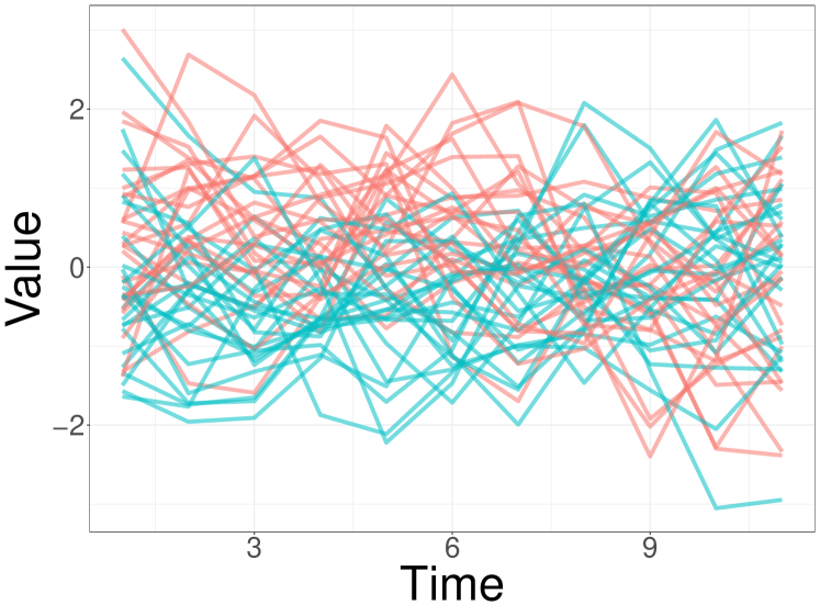
Figure 1: Failure of the Wald test. We sample 100 datasets following Model (1) with zero mean functions and zero noise terms ($\mu_{i}=0,\sigma_{j}^{2}=0$ for all $i,j\in[m]$). Each dataset contains 500 subjects, where the record for each subject contains 1 feature with 11 time points scattered uniformly in $[0,1]$ (i.e., $n=500$, $m=1$, $r_{ij}=11$ for all $i\in[500],j\in[1]$). For each dataset, we apply $k$-means to obtain two clusters. (a) shows the first 100 records of the first dataset labeled by the clustering outputs. (b) is the quantile plot of the $p$-values for the 100 datasets obtained by the Wald test.

3 Selective Inference for Functional Data Clustering

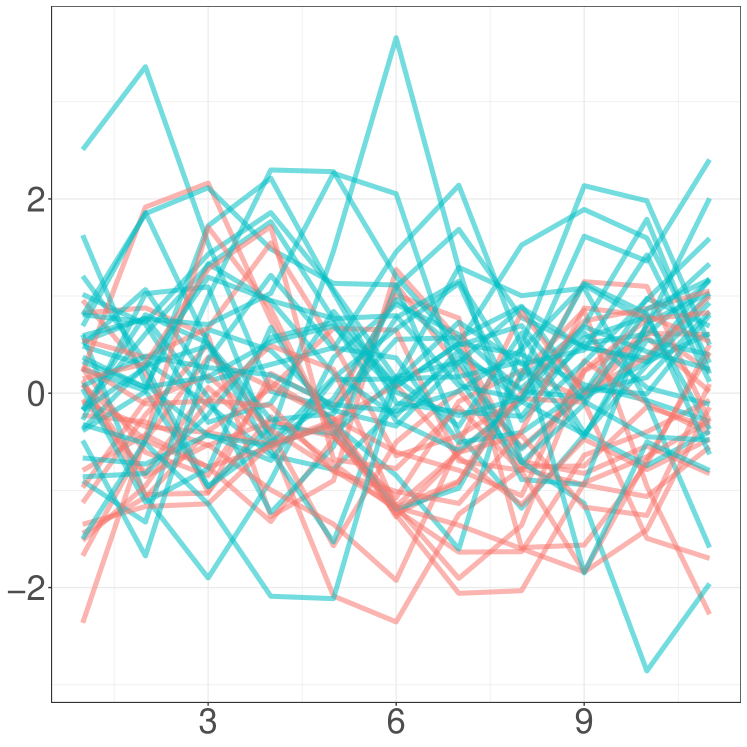
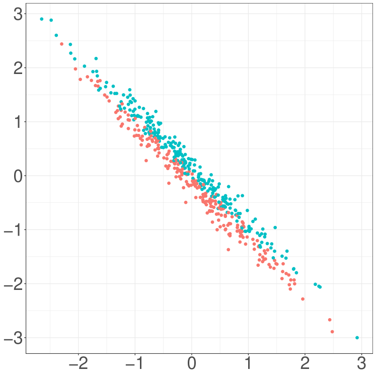
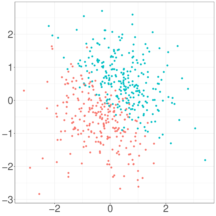
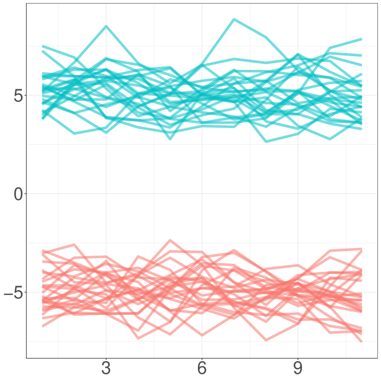
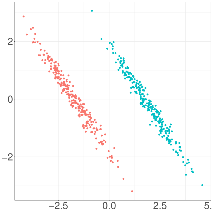
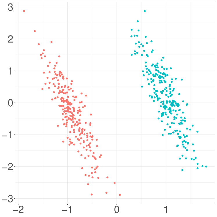
Figure 2: Overall procedure. (a). the first 100 curves of the dataset with the common mean $\mu_{i}=0$ and the zero noise $\epsilon_{i}=0$ labeled by the clustering results. (b). scatter plot (first two coordinates) of the low-dimensional embedding for this dataset. (c). scatter plot of the whitened data; (d). the first 100 curves of the dataset with the mean $\mu_{i}=-5$ or $\mu_{i}=5$ and the zero noise term labeled by the clustering results; (e). scatter plots (first two coordinates) for the low-dimensional embedding and whitened data; (f). scatter plots (first two coordinates) for the low-dimensional embedding and whitened data.

In this section, we introduce the procedure of PSIMF for testing the difference between post-clustering matrix data following Model (1) that addresses the challenges described in Section 2.2.

Our procedure is based on the selective inference framework, which adjusts the inferential process to account for the selection that has occurred, thereby providing statistically valid conclusions. In the context of our hypothesis test (2), we aim to test $\mu_{\mathcal{C}_{1}}=\mu_{\mathcal{C}_{2}}$ given $\mathcal{C}_{1},\mathcal{C}_{2}\in\mathcal{C}(w)$, where $w\coloneqq(w_{i})_{i\in[n]}$ is a random sample generated by Model (1). A natural approach is deriving the selection procedure by constructing a $p$-value conditioning on the clustering outputs $\mathcal{C}_{1}$ and $\mathcal{C}_{2}$. Specifically, in the special case where the time points of measurements $\Omega_{i}$ are consistent across all subjects, the selective $p$-value could be defined as follows:

$$\mathbb{P}_{H_{0}^{\{\mathcal{C}_{1},\mathcal{C}_{2}\}}}\left(\lVert\overline{W}_{\mathcal{C}_{1}}-\overline{W}_{\mathcal{C}_{2}}\rVert\geq\lVert\overline{w}_{\mathcal{C}_{1}}-\overline{w}_{\mathcal{C}_{2}}\rVert\Big{|}~{}\mathcal{C}_{1},\mathcal{C}_{2}\in\mathcal{C}(\mathcal{W})\right).$$ (4)

However, in practice, the time records $\Omega_{i}$ often differ across subjects, rendering the sample means $\overline{w}_{\mathcal{C}_{1}}$ and $\overline{w}_{\mathcal{C}_{2}}$ ill-defined, and the direct application of our initial approach (4) is infeasible. To overcome this, we transform $w_{i}$ into vectors with the same dimension by considering their low-dimensional representations through basis expansion regression. More details on this can be found in Section 3.1. Additionally, the $p$-value as initially defined is numerically infeasible due to the complexity of the condition $\{\mathcal{C}_{1},\mathcal{C}_{2}\in\mathcal{C}(\mathcal{W})\}$. In Section 3.3, we simplify this condition through an orthogonal decomposition and define a formal $p$-value.

Our method includes three main steps: first, we conduct the basis expansion regression to embed the functional data $W_{i}$ into low-dimensional vectors and form a tensor structure; second, we conduct the whitening transformation to normalize the tensor; third, we calculate the selective $p$-value on the tensor data leveraging the clustering information. We describe these three steps in the following Sections 3.1, 3.2, 3.3, respectively.

3.1 Low-dimensional Embedding

In this step, we aim to identify a low-dimensional representation of the functional data by embedding the multivariate Gaussian process data into a dimension-reduced tensor representation.

Recall Model (1), where $W_{ij}$ denotes the record of the $i$th subject and the $j$th feature. Given the time points $\Omega_{ij}$ and $(W_{ij}(t_{ijk}))_{k\in[r_{ij}]}\in\mathbb{R}^{r_{ij}}$, where $r_{ij}$ is the number of time points for this record. We select $q$ basis functions $\{\phi_{s}\}_{s\in[q]}$. Here, $q$ is a user-specified positive integer and each $\phi_{s}$ is Lipschitz continuous. We then perform the ridge regression as follows:

$$\alpha_{ij}\coloneqq\mathop{\arg\min}_{\alpha\in\mathbb{R}^{q}}\left\{\sum_{k=1}^{r_{ij}}\left(W_{ij}(t_{ijk})-\sum_{s=1}^{q}\alpha_{s}\cdot\phi_{s}(t_{ijk})\right)^{2}+\lambda\lVert\alpha\rVert^{2}\right\},$$ (5)

where $i\in[n]$, $j\in[m]$, $\lambda$ is a regularization parameter, and $(\phi_{s}(t_{ijk}))_{k\in[r_{ij}]}$ is a $r_{ij}$-dimensional vector of the basis function $\phi_{s}$. Define the matrix $\Phi_{ij}\coloneqq(\phi_{s}(t_{ijk}))_{s\in[q],k\in[r_{ij}]}\in\mathbb{R}^{q\times r_{ij}}$, where the $(s,k)$th entry of $\Phi_{ij}$ is $\phi_{s}(t_{ijk})$ for $s\in[q],k\in[r_{ij}]$. Define $K_{ij}\coloneqq\Phi_{ij}\Phi_{ij}^{\top}\in\mathbb{R}^{q\times q}$. Then, the coefficient vector $\alpha_{ij}$ has the following closed-form expression:

$$\alpha_{ij}=(K_{ij}+\lambda I_{q})^{-1}\Phi_{ij}(W_{ij}(t_{ijk}))_{k\in[r_{ij}]},$$ (6)

and the basis expansion function is $\widehat{\mu}_{ij}=\sum_{s=1}^{q}\alpha_{ijs}\phi_{s}$.

The linear transformation (6) embeds the functional data $W_{ij}$ into a $q$-dimensional vector $\alpha_{ij}$. By applying this low-dimensional embedding to all $i\in[n]$ and $j\in[m]$, we transform each $W_{ij}$ into an $m\times q$ matrix. Consequently, the entire dataset $\mathcal{W}$ is transformed into an $n\times m\times q$ tensor.

Definition 2 (Low-dimensional embedding).

Given the basis functions $\{\phi_{s}\}_{s\in[q]}$ and the time record $\Omega$, we define the linear map $H:\mathcal{W}\rightarrow\mathbb{R}^{n\times m\times q}$, where

$$H(\mathcal{W})[i,j,:]\coloneqq(K_{ij}+\lambda I_{q})^{-1}\Phi_{ij}(W_{ij}(t_{ijk}))_{k\in[r_{ij}]}.$$ (7)

The following lemma shows that under the distributional assumption, the vectorization of each slice $H(\mathcal{W})[i,:,:]\in\mathbb{R}^{m\times q}$ of the resulting tensor from Step 1 follows a multivariate normal distribution.

Lemma 1 (Distribution of $H(\mathcal{W})$).

Under Assumption 1, the following statements hold:

1. Define the block diagonal matrix $D_{i}\coloneqq{\rm diag}((K_{ij}+\lambda I_{q})^{-1}\Phi_{ij})_{j\in[m]}\in\mathbb{R}^{mq\times(\sum_{j=1}^{m}r_{ij})}$ and define $\mu_{ij}^{\Omega_{i}}\coloneqq(\mu_{ij}(t_{ijk}))_{k\in[r_{ij}]}$ as the vector of $\mu_{ij}$ characterized by the time record $\Omega_{i}$. For any $a,b\in[m]$, define $\Sigma_{ab}^{\Omega_{i}}=(R_{ab}(t_{ijk_{1}},t_{ijk_{2}}))_{k_{1},k_{2}\in[r_{ij}]}\in\mathbb{R}^{r_{ij}\times r_{ij}}$ as the covariance matrix, then

   $$\text{vec}\left(H(\mathcal{W})[i,:,:]\right)\sim\mathcal{N}\left\{\text{vec}\left[\left((K_{ij}+\lambda I_{q})^{-1}\Phi_{ij}\mu_{ij}^{\Omega_{i}}\right)_{j\in[m]}\right],D_{i}\left[\Sigma_{1}^{(i)}+\Sigma_{2}^{(i)}\right]D_{i}^{\top}\right\},$$ (8)

   where

   $$\Sigma_{1}^{(i)}\coloneqq\left(\Sigma_{ab}^{\Omega_{i}}\right)_{a,b\in[m]}\quad\text{and}\quad\Sigma_{2}^{(i)}\coloneqq{\rm diag}(\sigma_{j}^{2}\cdot I_{r_{ij}})_{j\in[m]}.$$

2. For some $i\in[n]$, if the number of time points $r_{ij}$ goes to infinite for all $j\in[m]$, then the distribution of $\text{vec}(H(\mathcal{W})[i,:,:])$ converges as follow:

   $$\text{vec}\left(H(\mathcal{W})[i,:,:]\right)\stackrel{{\scriptstyle d}}{{\longrightarrow}}\mathcal{N}\left\{\text{vec}\left(\left(K^{-1}\mu_{ij}^{(0)}\right)_{j\in[m]}\right),\Lambda\right\}\quad\text{as}\quad\min_{j\in[m]}r_{ij}\rightarrow\infty.$$ (9)

   Here,

   $$K\coloneqq\left(\int_{0}^{1}\phi_{s_{1}}(t)\phi_{s_{2}}(t)dt\right)_{s_{1},s_{2}\in[q]},\mu_{ij}^{(0)}\coloneqq\left(\int_{0}^{1}\phi_{s}(t)\mu_{ij}(t)dt\right)_{s\in[q]},\Lambda\coloneqq(\Lambda_{ab})_{a,b\in[m]}.$$

   We assume $K$ is invertible and define

   $$\Lambda_{ab}\coloneqq K^{-1}\left(\int_{0}^{1}\int_{0}^{1}\phi_{s_{1}}(t_{1})\phi_{s_{2}}(t_{2})(R_{ab}(t_{1},t_{2})+\mathbbm{1}_{a=b}\cdot\sigma_{a}^{2})dt_{1}dt_{2}\right)_{s_{1},s_{2}\in[q]}K^{-1}.$$

Proof.

See Appendix B.1. ∎

3.2 Whitening Transformation

Next, we perform the whitening transformation to normalize $H(\mathcal{W})$ obtained in Step 1. The goal is to transform the covariance matrix of distribution (8) into an identity matrix.

Define $\beta_{(i)}^{\Omega_{i}}\coloneqq\left((K_{ij}+\lambda I_{q}\right)^{-1}\Phi_{ij}\mu_{ij}^{\Omega_{i}})_{j\in[m]}$ and $\Lambda_{(i)}\coloneqq D_{i}\left[\Sigma_{1}^{(i)}+\Sigma_{2}^{(i)}\right]D_{i}^{\top}$. Then the distribution of (8) reduces to $\text{vec}\left(H(\mathcal{W})[i,:,:]\right)\sim\mathcal{N}\left(\text{vec}(\beta_{(i)}^{\Omega_{i}}),\Lambda_{(i)}\right)$. We introduce a slice-wise transformation $L$ on the tensor $H(\mathcal{W})$:

$$\text{vec}(L(\mathcal{W})[i,:,:])\coloneqq\Lambda_{(i)}^{-\frac{1}{2}}\text{vec}(H(\mathcal{W})[i,:,:]),\quad i=1,\ldots,n.$$ (10)

Under the distributional assumption, the transformed tensor follows another normal distribution:

$$\text{vec}(L(\mathcal{W})[i,:,:])\sim\mathcal{N}\left\{\Lambda_{(i)}^{-\frac{1}{2}}\text{vec}(\beta_{(i)}^{\Omega_{i}}),I_{mq}\right\},\quad i=1,\ldots,n.$$

Analogous to Lemma 1, we can characterize the asymptotic distribution of $\text{vec}(L(\mathcal{W})[i,:,:])$:

$$\text{vec}(L(\mathcal{W})[i,:,:])\stackrel{{\scriptstyle d}}{{\longrightarrow}}\mathcal{N}(\Lambda^{-\frac{1}{2}}\text{vec}(\beta_{(i)}),I_{mq})\quad\text{as}\quad\min_{j\in[m]}r_{ij}\rightarrow\infty,$$ (11)

where $\beta_{(i)}\coloneqq(K^{-1}\mu_{ij}^{(0)})_{j\in[m]}$ and $K,\Lambda,\mu_{ij}^{(0)}$ are defined in Lemma 1.

Covariance Estimation.

In practice, both the covariance function $R$ and the variance of noise $\sigma_{j}^{2}$ are typically unknown, rendering the covariance matrix $\Lambda$ unknown. Therefore, we apply the following sample covariance estimator to estimate $\Lambda$:

$$\widehat{\Lambda}\coloneqq\frac{1}{n-1}\left[\sum_{i=1}^{n}\left(\text{vec}(H(\mathcal{W})[i,:,:])-\text{vec}(\overline{H(\mathcal{W})})\right)\left(\text{vec}(H(\mathcal{W})[i,:,:]-\text{vec}(\overline{H(\mathcal{W})})\right)^{\top}\right],$$

where $\overline{H(\mathcal{W})}\coloneqq\sum_{i=1}^{n}H(\mathcal{W})[i,:,:]/n$ is the sample mean.

If the null hypothesis $H_{0}^{\{\mathcal{C}_{1},\mathcal{C}_{2}\}}$ holds (i.e., $\mu_{\mathcal{C}_{1}}=\mu_{\mathcal{C}_{2}}$), we have $\mu_{i_{1}}=\mu_{i_{2}}$ and $\beta_{(i_{1})}=\beta_{(i_{2})}$ for all $i_{1},i_{2}\in[n]$. Lemma 1 implies that $\text{vec}(H(\mathcal{W})[i,:,:])\sim\mathcal{N}(\text{vec}(\beta_{(i)}),\Lambda)$ as $r_{ij}\rightarrow\infty$ for all $j\in[m]$. Therefore, if $H_{0}^{\{\mathcal{C}_{1},\mathcal{C}_{2}\}}$ holds and the sample size $n\rightarrow\infty$, we have $\widehat{\Lambda}\stackrel{{\scriptstyle p}}{{\longrightarrow}}\Lambda$.

If the alternative hypothesis $H_{1}^{\{\mathcal{C}_{1},\mathcal{C}_{2}\}}$ holds (i.e., $\mu_{\mathcal{C}_{1}}\neq\mu_{\mathcal{C}_{2}}$), define

$$\beta_{\mathcal{C}_{j}}\coloneqq\beta_{(i)}\quad\text{for some}\quad i\in\mathcal{C}_{j}\quad\text{and}\quad j\in\{1,2\},$$

then we have $\beta_{\mathcal{C}_{1}}\neq\beta_{\mathcal{C}_{2}}$. In this situation, we rewrite the sample covariance estimator as follows:

$$\widehat{\Lambda} =\bigg{(}\sum_{j=1}^{2}\bigg{[}\sum_{i\in\mathcal{C}_{j}}(\text{vec}(H(\mathcal{W})[i,:,:])-\text{vec}(\overline{H(\mathcal{W})}_{\mathcal{C}_{j}}))(\text{vec}(H(\mathcal{W})[i,:,:])-\text{vec}(\overline{H(\mathcal{W})}_{\mathcal{C}_{j}}))^{\top}$$ (12)

$$+|\mathcal{C}_{j}|(\text{vec}(\overline{H(\mathcal{W})}_{\mathcal{C}_{j}})-\text{vec}(\overline{H(\mathcal{W})}))(\text{vec}(\overline{H(\mathcal{W})}_{\mathcal{C}_{j}})-\text{vec}(\overline{H(\mathcal{W})}))^{\top}\bigg{]}\bigg{)}/(n-1).$$

Intuitively, (12) implies that

$$\widehat{\Lambda}\stackrel{{\scriptstyle p}}{{\longrightarrow}}\Lambda+\frac{c}{(c+1)^{2}}\text{vec}(\beta_{\mathcal{C}_{1}}-\beta_{\mathcal{C}_{2}})\cdot\text{vec}(\beta_{\mathcal{C}_{1}}-\beta_{\mathcal{C}_{2}})^{\top}$$ (13)

as $|\mathcal{C}_{1}|,|\mathcal{C}_{2}|\rightarrow\infty$, $|\mathcal{C}_{1}|/|\mathcal{C}_{2}|\rightarrow c$, and $r_{ij}\rightarrow\infty$. Therefore, the sample covariance estimator $\widehat{\Lambda}$ has a constant bias $c/(c+1)^{2}\cdot\text{vec}(\beta_{\mathcal{C}_{1}}-\beta_{\mathcal{C}_{2}})\cdot\text{vec}(\beta_{\mathcal{C}_{1}}-\beta_{\mathcal{C}_{2}})^{\top}$. In Section 4, we leverage this bias to show that the proposed estimator controls the statistical power under mild additional assumptions.

3.3 Selective $p$-value

Suppose $w=(w_{i})_{i\in[n]}$ is a sample generated from Model (1) and $L(w)$ is a tensor obtained by low-dimensional embedding and whitening transformation. Next, we apply a clustering algorithm (such as the hierarchical clustering or $k$-means clustering) on $\{L(w)[i,:,:]\}_{i\in[n]}$ to separate $n$ subjects into two clusters, where the indices are denoted by $\mathcal{C}_{1},\mathcal{C}_{2}$, respectively. Analogous to (4), we consider the following selective $p$-value that leverages the clustering information:

$$\mathbb{P}_{H_{0}^{\{\mathcal{C}_{1},\mathcal{C}_{2}\}}}\left(\lVert\overline{L(\mathcal{W})}_{\mathcal{C}_{1}}-\overline{L(\mathcal{W})}_{\mathcal{C}_{2}}\rVert_{F}\geq\lVert\overline{L(w)}_{\mathcal{C}_{1}}-\overline{L(w)}_{\mathcal{C}_{2}}\rVert_{F}\Big{|}~{}\mathcal{C}_{1},\mathcal{C}_{2}\in\mathcal{C}(L(\mathcal{W}))\right),$$ (14)

where $\overline{L(\mathcal{W})}_{\mathcal{C}_{j}}\coloneqq\sum_{i\in\mathcal{C}_{j}}L(\mathcal{W})[i,:,:]/|\mathcal{C}_{j}|$ for all $j\in\{1,2\}$. We remark that the clustering algorithm $\mathcal{C}(\cdot)$ is implemented on a collection of matrix data $\{L(w)[i,:,:]\}_{i\in[n]}$ instead of the functional data $\mathcal{W}$. Intuitively, the proposed $p$-value is a probability of $L(\mathcal{W})$ conditioning on the region $\{L(\mathcal{W}):\mathcal{C}_{1},\mathcal{C}_{2}\in\mathcal{C}(L(\mathcal{W}))\}$. Following the selective inference theory (Fithian et al., 2014), this selective $p$-value leverages the model selection information to eliminate the selection bias and further control the selective type-I error.

Definition 3.

(Post-clustering selective type-I error). Suppose that $\mathcal{W}=(W_{i})_{i\in[n]}$ follows Model (1) and $w$ is a realization of $\mathcal{W}$. Suppose that the partition $\mathcal{C}_{1},\mathcal{C}_{2}$ ($\mathcal{C}_{1}\cup\mathcal{C}_{2}=[n]$, $\mathcal{C}_{1}\cap\mathcal{C}_{2}=\emptyset$) is the output of a clustering algorithm $\mathcal{C}(\cdot)$. Let $H_{0}^{\{\mathcal{C}_{1},\mathcal{C}_{2}\}}$ be the null hypothesis defined as (2), we say a test of $H_{0}^{\{\mathcal{C}_{1},\mathcal{C}_{2}\}}$ based on $\mathcal{W}$ controls the selective type-I error for clustering at level $\alpha$ if

$$\mathbb{P}_{H_{0}^{\{\mathcal{C}_{1},\mathcal{C}_{2}\}}}\left(\text{reject $H_{0}^{\{\mathcal{C}_{1},\mathcal{C}_{2}\}}$ based on $\mathcal{W}$ at level $\alpha$}\Big{|}~{}\mathcal{C}_{1},\mathcal{C}_{2}\in\mathcal{C}(L(\mathcal{W}))\right)\leq\alpha$$ (15)

for any $\alpha\in[0,1]$.

However, the selective $p$-value (14) cannot be directly calculated because the condition $\mathcal{C}_{1},\mathcal{C}_{2}\in\mathcal{C}(L(\mathcal{W}))$ is numerically infeasible, meaning the selection set $\{L(\mathcal{W}):\mathcal{C}_{1},\mathcal{C}_{2}\in\mathcal{C}(L(\mathcal{W}))\}$ might be complex and difficult to construct. Inspired by the approach in Lucy L. Gao and Witten (2024), we aim to modify the selection set to simplify the expression of the selective $p$-value. Given the clustering output $\mathcal{C}_{1},\mathcal{C}_{2}$, we define the indicator vector as follows:

$$\nu(\mathcal{C}_{1},\mathcal{C}_{2})\coloneqq\left(\frac{\mathbbm{1}_{\{i\in\mathcal{C}_{1}\}}}{|\mathcal{C}_{1}|}-\frac{\mathbbm{1}_{\{i\in\mathcal{C}_{2}\}}}{|\mathcal{C}_{2}|}\right)_{i\in[n]},$$

where the $i$th coordinate of $\nu(\mathcal{C}_{1},\mathcal{C}_{2})$ is $1/|\mathcal{C}_{1}|$ if $i\in\mathcal{C}_{1}$ and $-1/|\mathcal{C}_{2}|$ if $i\in\mathcal{C}_{2}$. Based on $\nu(\mathcal{C}_{1},\mathcal{C}_{2})$, we decouple $L(\mathcal{W})$ by the following orthogonal decomposition.

Lemma 2.

(Orthogonal Decomposition). For any tensor $\mathcal{A}\in\mathbb{R}^{n\times m\times q}$ and any partition of $[n]$ denoted by $\mathcal{C}_{1},\mathcal{C}_{2}$, we have the following decomposition:

$$\mathcal{A}=\pi^{\perp}_{\nu(\mathcal{C}_{1},\mathcal{C}_{2})}\times_{1}\mathcal{A}+\left(\frac{\lVert\overline{\mathcal{A}}_{\mathcal{C}_{1}}-\overline{\mathcal{A}}_{\mathcal{C}_{2}}\rVert_{F}}{1/|\mathcal{C}_{1}|+1/|\mathcal{C}_{2}|}\right)\nu(\mathcal{C}_{1},\mathcal{C}_{2})\times_{1}\text{dir}(\overline{\mathcal{A}}_{\mathcal{C}_{1}}-\overline{\mathcal{A}}_{\mathcal{C}_{2}})^{\top},$$ (16)

where $\overline{\mathcal{A}}_{\mathcal{C}_{i}}=\sum_{j\in\mathcal{C}_{i}}\mathcal{A}[j,:,:]/|\mathcal{C}_{i}|$ is the mean of mode-1 slices corresponding to the partition $\mathcal{C}_{i}$, $\times_{1}$ denotes the tensor mode-1 product (here we view $\nu(\mathcal{C}_{1},\mathcal{C}_{2})$ as a $n\times 1$ matrix and $\text{dir}(\overline{\mathcal{A}}_{\mathcal{C}_{1}}-\overline{\mathcal{A}}_{\mathcal{C}_{2}})$ as a $1\times m\times q$ tensor), $\pi^{\perp}_{\nu}=I-\frac{\nu\nu^{\top}}{\lVert\nu\rVert^{2}}$ is an orthogonal projection matrix, and $\text{dir}(\omega)=\frac{\omega}{\lVert\omega\rVert_{F}}\mathbbm{1}_{\{\omega\neq 0\}}$ is the direction of $\omega$ (here $\omega$ is a matrix, $\lVert\omega\rVert_{F}$ is its Frobenius norm, and $\mathbbm{1}_{\{\omega\neq 0\}}$ is the indicator function takes the value $0$ when all the entries in $\omega$ are zero and takes the value $1$ otherwise).

Proof.

See Appendix B.2. ∎

Plugging $L(\mathcal{W})$ into Lemma 2, we have

$$L(\mathcal{W})=\pi^{\perp}_{\nu(\mathcal{C}_{1},\mathcal{C}_{2})}\times_{1}L(\mathcal{W})+\left[\frac{\lVert\overline{L(\mathcal{W})}_{\mathcal{C}_{1}}-\overline{L(\mathcal{W})}_{\mathcal{C}_{2}}\rVert_{F}}{1/|\mathcal{C}_{1}|+1/|\mathcal{C}_{2}|}\right]\nu(\mathcal{C}_{1},\mathcal{C}_{2})\times_{1}\text{dir}\left(\overline{L(\mathcal{W})}_{\mathcal{C}_{1}}-\overline{L(\mathcal{W})}_{\mathcal{C}_{2}}\right)^{\top}.$$

Based on this decomposition of $L(\mathcal{W})$, we define the following selective $p$-value incorporating additional conditions.

Definition 4.

(Selective $p$-value). Suppose that $\mathcal{W}$ follows Model (1) and $w$ is a realization of $\mathcal{W}$. Suppose that the partition $\mathcal{C}(L(w))=\{\mathcal{C}_{1},\mathcal{C}_{2}\}$ ($\mathcal{C}_{1}\cup\mathcal{C}_{2}=[n],\mathcal{C}_{1}\cap\mathcal{C}_{2}=\emptyset$) is the output of a clustering algorithm $\mathcal{C}(\cdot)$. Let $H_{0}^{\{\mathcal{C}_{1},\mathcal{C}_{2}\}}$ be the null hypothesis defined as (2), we propose the following selective $p$-value:

$$p_{selective}=\mathbb{P}_{H_{0}^{\{\mathcal{C}_{1},\mathcal{C}_{2}\}}}\bigg{(}\lVert\overline{L(\mathcal{W})}_{\mathcal{C}_{1}}-\overline{L(\mathcal{W})}_{\mathcal{C}_{2}}\rVert_{F}\geq\lVert\overline{L(w)}_{\mathcal{C}_{1}}-\overline{L(w)}_{\mathcal{C}_{2}}\rVert_{F}\bigg{|}\mathcal{C}_{1},\mathcal{C}_{2}\in\mathcal{C}(L(\mathcal{W})),$$ (17)

$$\pi^{\perp}_{\nu(\mathcal{C}_{1},\mathcal{C}_{2})}\times_{1}L(\mathcal{W})=\pi^{\perp}_{\nu(\mathcal{C}_{1},\mathcal{C}_{2})}\times_{1}L(w),\text{dir}(\overline{L(\mathcal{W})}_{\mathcal{C}_{1}}-\overline{L(\mathcal{W})}_{\mathcal{C}_{2}})=\text{dir}(\overline{L(w)}_{\mathcal{C}_{1}}-\overline{L(w)}_{\mathcal{C}_{2}})\bigg{)}.$$

Under the null hypothesis $H_{0}^{\{\mathcal{C}_{1},\mathcal{C}_{2}\}}$, we have $\sum_{i\in\mathcal{C}_{1}}\beta_{(i)}/|\mathcal{C}_{1}|=\sum_{i\in\mathcal{C}_{2}}\beta_{(i)}/|\mathcal{C}_{2}|$, then (11) implies that

$$\text{vec}\left(\overline{L(\mathcal{W})}_{\mathcal{C}_{1}}-\overline{L(\mathcal{W})}_{\mathcal{C}_{2}}\right)\stackrel{{\scriptstyle d}}{{\longrightarrow}}\sqrt{1/|\mathcal{C}_{1}|+1/|\mathcal{C}_{2}|}\cdot\mathcal{N}(0,I_{mq})\quad\text{as}\quad\min_{i\in[n],j\in[m]}r_{ij}\rightarrow\infty.$$ (18)

Next, we plug in (18) to reform the selective $p$-value (17). To elaborate, (18) implies that $\lVert\overline{L(\mathcal{W})}_{\mathcal{C}_{1}}-\overline{L(\mathcal{W})}_{\mathcal{C}_{2}}\rVert_{F}$ follows the distribution $\sqrt{1/|\mathcal{C}_{1}|+1/|\mathcal{C}_{2}|}\cdot\chi_{mq}$ if the null hypothesis holds (and the number of time points goes to infinite). Therefore, we can reform the selective $p$-value as a survival function of a truncated chi-squared distribution.

Lemma 3.

Suppose that $\mathcal{W}$ follows Model (1) and $w$ is a realization of $\mathcal{W}$. Suppose that $\text{vec}(\overline{L(\mathcal{W})}_{\mathcal{C}_{1}}-\overline{L(\mathcal{W})}_{\mathcal{C}_{2}})\sim\sqrt{1/|\mathcal{C}_{1}|+1/|\mathcal{C}_{2}|}\cdot\mathcal{N}(0,I_{mq})$. Then the selective $p$-value (17) can be rewritten as follows:

$$p_{selective}=1-\mathbb{F}\left(\lVert\overline{L(w)}_{\mathcal{C}_{1}}-\overline{L(w)}_{\mathcal{C}_{2}}\rVert_{F};\sqrt{\frac{1}{|\mathcal{C}_{1}|}+\frac{1}{|\mathcal{C}_{2}|}},\mathcal{S}(w;\mathcal{C}_{1},\mathcal{C}_{2})\right),$$ (19)

where $\mathbb{F}(t;c,\mathcal{S})$ denotes the cumulative distribution function of the random variable $c\cdot\chi_{mq}$ truncated to the set $\mathcal{S}$ defined by

$$\begin{split}&\mathcal{S}(w;\mathcal{C}_{1},\mathcal{C}_{2})\coloneqq\Bigg{\{}\varphi\geq 0:\\ &\quad\mathcal{C}_{1},\mathcal{C}_{2}\in\mathcal{C}\Big{(}\pi^{\perp}_{\nu(\mathcal{C}_{1},\mathcal{C}_{2})}\times_{1}L(w)+\left[\frac{\varphi}{1/|\mathcal{C}_{1}|+1/|\mathcal{C}_{2}|}\right]\nu(\mathcal{C}_{1},\mathcal{C}_{2})\times_{1}\text{dir}(\overline{L(w)}_{\mathcal{C}_{1}}-\overline{L(w)}_{\mathcal{C}_{2}})^{\top}\Big{)}\Bigg{\}}.\end{split}$$

Proof.

See Appendix B.3. ∎

3.4 Numerical Approximation of Selective $p$-value

Now we introduce the Monte Carlo method to compute the truncated survival function (19), which serves as an approximation of the selective $p$-value (17).

To begin with, we briefly discuss the geometric intuition of $\mathcal{S}(w;\mathcal{C}_{1},\mathcal{C}_{2})$. Given a partition $\mathcal{C}_{1},\mathcal{C}_{2}$ obtained by a certain clustering algorithm, we consider the linear map $F:\mathbb{R}\rightarrow\mathbb{R}^{n\times m\times q}$:

$$F(\varphi)\coloneqq\pi^{\perp}_{\nu(\mathcal{C}_{1},\mathcal{C}_{2})}\times_{1}L(w)+\left[\frac{\varphi}{1/|\mathcal{C}_{1}|+1/|\mathcal{C}_{2}|}\right]\nu(\mathcal{C}_{1},\mathcal{C}_{2})\times_{1}\text{dir}\left(\overline{L(w)}_{\mathcal{C}_{1}}-\overline{L(w)}_{\mathcal{C}_{2}}\right)^{\top}.$$ (20)

Intuitively speaking, $F$ operates the orthogonal projection $\pi^{\perp}_{\nu(\mathcal{C}_{1},\mathcal{C}_{2})}\times_{1}L(w)$ along a “vector” $\nu(\mathcal{C}_{1},\mathcal{C}_{2})\times_{1}\text{dir}\left(\overline{L(w)}_{\mathcal{C}_{1}}-\overline{L(w)}_{\mathcal{C}_{2}}\right)^{\top}$ with the length $\varphi$. The set $\mathcal{S}(w;\mathcal{C}_{1},\mathcal{C}_{2})$ contains all the “length” $\varphi\in\mathbb{R}$ such that the transformed tensor has the same clustering outputs as $L(w)$ (i.e., the partition is equal to $\mathcal{C}_{1},\mathcal{C}_{2}$). Lemma 2 shows

$$L(w)=\pi^{\perp}_{\nu(\mathcal{C}_{1},\mathcal{C}_{2})}\times_{1}L(w)+\left[\frac{\lVert\overline{L(w)}_{\mathcal{C}_{1}}-\overline{L(w)}_{\mathcal{C}_{2}}\rVert_{F}}{1/|\mathcal{C}_{1}|+1/|\mathcal{C}_{2}|}\right]\nu(\mathcal{C}_{1},\mathcal{C}_{2})\times_{1}\text{dir}\left(\overline{L(w)}_{\mathcal{C}_{1}}-\overline{L(w)}_{\mathcal{C}_{2}}\right)^{\top}.$$

Therefore, we conclude that $\lVert\overline{L(w)}_{\mathcal{C}_{1}}-\overline{L(w)}_{\mathcal{C}_{2}}\rVert_{F}\in\mathcal{S}(w;\mathcal{C}_{1},\mathcal{C}_{2})$. Furthermore, when $\varphi>\mathcal{S}(w;\mathcal{C}_{1},\mathcal{C}_{2})$, the transformation $F$ “pushes away” the sets $\{L(w)[i,:,:]\}_{i\in\mathcal{C}_{1}}$ and $\{L(w)[i,:,:]\}_{i\in\mathcal{C}_{2}}$ along the vector $\nu(\mathcal{C}_{1},\mathcal{C}_{2})\times_{1}\text{dir}(\overline{L(w)}_{\mathcal{C}_{1}}-\overline{L(w)}_{\mathcal{C}_{2}})^{\top}$, and vice versa. If $\varphi$ is too large or small, the clustering output of $F(\varphi)$ will be different from $\mathcal{C}_{1},\mathcal{C}_{2}$. Therefore, $\mathcal{S}(w;\mathcal{C}_{1},\mathcal{C}_{2})$ concentrates near $\lVert\overline{L(w)}_{\mathcal{C}_{1}}-\overline{L(w)}_{\mathcal{C}_{2}}\rVert_{F}$.

Monte Carlo Approximation.

We use the Monte Carlo method to approximate (19), which is the survival function of the distribution $\sqrt{1/|\mathcal{C}_{1}|+1/|\mathcal{C}_{2}|}\cdot\chi_{mq}$ truncated on the set $\mathcal{S}(w;\mathcal{C}_{1},\mathcal{C}_{2})$. Mathematically, we rewrite (19) as follows:

$$\begin{split}p_{selective}=&\frac{\mathbb{P}\left(\varphi\geq\lVert\overline{L(w)}_{\mathcal{C}_{1}}-\overline{L(w)}_{\mathcal{C}_{2}}\rVert_{F},\mathcal{C}_{1},\mathcal{C}_{2}\in\mathcal{C}(F(\varphi))\right)}{\mathbb{P}(\mathcal{C}_{1},\mathcal{C}_{2}\in\mathcal{C}(F(\varphi)))}\\ =&\frac{\mathbb{E}\left[\mathbbm{1}_{\{\varphi\geq\lVert\overline{L(w)}_{\mathcal{C}_{1}}-\overline{L(w)}_{\mathcal{C}_{2}}\rVert_{F},\mathcal{C}_{1},\mathcal{C}_{2}\in\mathcal{C}(F(\varphi))\}}\right]}{\mathbb{E}[\mathbbm{1}_{\{\mathcal{C}_{1},\mathcal{C}_{2}\in\mathcal{C}(F(\varphi))\}}]},\end{split}$$

where $\varphi$ follows the distribution $\sqrt{1/|\mathcal{C}_{1}|+1/|\mathcal{C}_{2}|}\cdot\chi_{mq}$, $\mathbb{P}$ is the corresponding probability mass function, and $\mathbb{E}$ is the expectation with respect to $\varphi$. We will sample some $\varphi\in\mathbb{R}$ and check if $\varphi\in\mathcal{S}(w;\mathcal{C}_{1},\mathcal{C}_{2})$ to approximate $\mathcal{S}(w;\mathcal{C}_{1},\mathcal{C}_{2})$ and further estimate $p_{selective}$.

We apply importance sampling to approximate this conditional probability. As aforementioned, $\mathcal{S}(w;\mathcal{C}_{1},\mathcal{C}_{2})$ concentrates near $\lVert\overline{L(w)}_{\mathcal{C}_{1}}-\overline{L(w)}_{\mathcal{C}_{2}}\rVert_{F}$. Therefore, we set $g(x)=f_{1}(x)/f_{2}(x)$, where $f_{1}$ is the density of $\sqrt{1/|\mathcal{C}_{1}|+1/|\mathcal{C}_{2}|}\cdot\chi_{mq}$ and $f_{2}$ is the density function of $\mathcal{N}\left(\lVert\overline{L(w)}_{\mathcal{C}_{1}}-\overline{L(w)}_{\mathcal{C}_{2}}\rVert_{F},1/|\mathcal{C}_{1}|+1/|\mathcal{C}_{2}|\right)$. For a positive integer $S$, we sample $S$ values $\gamma_{1},\ldots,\gamma_{S}\sim\mathcal{N}(\lVert\overline{L(w)}_{\mathcal{C}_{1}}-\overline{L(w)}_{\mathcal{C}_{2}}\rVert_{F},1/|\mathcal{C}_{1}|+1/|\mathcal{C}_{2}|)$, then the selective $p$-value can be approximately by

$$p_{selective}\approx\frac{\sum\pi_{i}\mathbbm{1}_{\{\gamma_{i}\geq\lVert\overline{L(w)}_{\mathcal{C}_{1}}-\overline{L(w)}_{\mathcal{C}_{2}}\rVert_{F},\mathcal{C}_{1},\mathcal{C}_{2}\in\mathcal{C}(F(\gamma_{i}))\}}}{\sum\pi_{i}\mathbbm{1}_{\{\mathcal{C}_{1},\mathcal{C}_{2}\in\mathcal{C}(F(\gamma_{i}))\}}},~{}~{}~{}~{}\pi_{i}=\frac{f_{1}(\gamma_{i})}{f_{2}(\gamma_{i})}.$$ (21)

3.5 Overall Procedures

We summarize the three steps for computing the selective $p$-value as an overall procedure PSIMF in Algorithm 1.

Step I: Low-dimensional embedding;

Input: Data of $n$ subjects $\mathcal{W}$, time record $\Omega$, basis functions $\{\phi_{s}\}_{s\in[q]}$, regularization term $\lambda$.

1. Compute the matrices $K_{ij}$ and $\Phi_{ij}$ by $\Omega$ and $\{\phi_{s}\}_{s\in[q]}$;

2. (Basis expansion regression). $X_{i}\leftarrow(K_{ij}+\lambda I_{q})^{-1}\Phi_{ij}W_{ij}$, for $i\in[n]$;

Output: Low-dimensional embedding $\{X_{i}\}_{i\in[n]}$.

Step II: Covariance estimation;

Input: Low-dimensional embedding $\{X_{i}\}_{i\in[n]}$.

3. Compute the sample covariance $\widehat{\Lambda}\coloneqq\frac{\sum_{i=1}^{n}(\text{vec}(X_{i})-\text{vec}(\overline{X}))(\text{vec}(X_{i})-\text{vec}(\overline{X}))^{\top}}{n-1}$;

Output: Estimated covariance matrix $\widehat{\Lambda}$.

Step III: Whitening and Clustering;

Input: Low-dimensional embedding $\{X_{i}\}_{i\in[n]}$, covariance matrix $\widehat{\Lambda}$.

4. (Whitening). Conduct the linear transformation $\text{vec}(Y_{i})\leftarrow(\widehat{\Lambda})^{-\frac{1}{2}}\text{vec}(X_{i})$;

5. (Clustering). Apply certain clustering algorithm on $\{Y_{i}\}_{i\in[n]}$ and obtain a partition $\mathcal{C}_{1},\mathcal{C}_{2}$, where the number of clusters is $2$;

Output: Whitened data $\{Y_{i}\}_{i\in[n]}$, partition $\mathcal{C}_{1},\mathcal{C}_{2}$.

Step IV: Numerical approximation of the selective $p$-value;

Input: Whitened data $\{Y_{i}\}_{i\in[n]}$, partition $\mathcal{C}_{1},\mathcal{C}_{2}$, sampling horizon $S$.

for $s=1\to S$ do

       6. Generate $\gamma_{s}\sim\sqrt{1/|\mathcal{C}_{1}|+1/|\mathcal{C}_{2}|}\cdot\chi_{mq}$, compute $\pi_{s}=f_{1}(\gamma_{s})/f_{2}(\gamma_{s})$;

       7. Apply the same clustering algorithm to obtain the partition $\mathcal{C}(F(\gamma_{s}))$;

      

end for

Output: Selective $p$-value $\frac{\sum_{s=1}^{S}\pi_{s}\mathbbm{1}_{\{\omega_{s}\geq\lVert\overline{Y}_{\mathcal{C}_{1}}-\overline{Y}_{\mathcal{C}_{2}}\rVert,\mathcal{C}_{1},\mathcal{C}_{2}\in\mathcal{C}(F(\gamma_{s}))\}}}{\sum_{s=1}^{S}\pi_{s}\mathbbm{1}_{\{\mathcal{C}_{1},\mathcal{C}_{2}\in\mathcal{C}(F(\gamma_{s}))\}}}$.

Algorithm 1 Post Selective Inference for Multiple Functional Data (PSIMF)

4 Theoretical Guarantees

In this section, we present theoretical results for PSIMF. We first focus on the selective type-I error. Recall that the selective $p$-value is the survival function of a truncated chi-squared distribution. Therefore, if the selective $p$-value conditioning on the selection set follows a uniform distribution on $[0,1]$, then the selective type-I error can be controlled accordingly. The following theorem provides a formal statement:

Theorem 1.

(Selective Type-I error control). Suppose $\mathcal{W}$ follows Model (1) and $w$ is a realization of $\mathcal{W}$. Suppose the partition $\mathcal{C}(L(w))=\{\mathcal{C}_{1},\mathcal{C}_{2}\}$ ($\mathcal{C}_{1}\cup\mathcal{C}_{2}=[n],\mathcal{C}_{1}\cap\mathcal{C}_{2}=\emptyset$) is the output of the clustering algorithm $\mathcal{C}(\cdot)$. Suppose $\text{vec}(\overline{L(\mathcal{W})}_{\mathcal{C}_{1}}-\overline{L(\mathcal{W})}_{\mathcal{C}_{2}})\sim\sqrt{1/|\mathcal{C}_{1}|+1/|\mathcal{C}_{2}|}\cdot\mathcal{N}(0,I_{mq})$ if the null hypothesis $H_{0}^{\{\mathcal{C}_{1},\mathcal{C}_{2}\}}$ holds, then the selective type-I error is controlled by $\alpha\in[0,1]$:

$$\mathbb{P}_{H_{0}^{\{\mathcal{C}_{1},\mathcal{C}_{2}\}}}\left(p(\mathcal{W};\mathcal{C}_{1},\mathcal{C}_{2})\leq\alpha\big{|}~{}\mathcal{C}_{1},\mathcal{C}_{2}\in\mathcal{C}(L(\mathcal{W}))\right)=\alpha,$$ (22)

where $p(\mathcal{W};\mathcal{C}_{1},\mathcal{C}_{2})$ denotes the selective $p$-value given the data $\mathcal{W}$ and the partition $\{\mathcal{C}_{1},\mathcal{C}_{2}\}$.

Proof.

See Appendix A.1. ∎

Next, we study the statistical power of PSIMF, beginning with an intuitive analysis. Under the alternative hypothesis $H_{1}^{\{\mathcal{C}_{1},\mathcal{C}_{2}\}}$, if $|\mathcal{C}_{1}|,|\mathcal{C}_{2}|\rightarrow\infty$, $|\mathcal{C}_{1}|/|\mathcal{C}_{2}|\rightarrow c\in(0,1)$, (13) implies that as $n\rightarrow\infty$,

$$\widehat{\Lambda}\stackrel{{\scriptstyle p}}{{\longrightarrow}}\Lambda+\frac{c}{(c+1)^{2}}\text{vec}(\beta_{\mathcal{C}_{1}}-\beta_{\mathcal{C}_{2}})\cdot\text{vec}(\beta_{\mathcal{C}_{1}}-\beta_{\mathcal{C}_{2}})^{\top}.$$

Also, suppose there are infinitely many time points, i.e., $\min_{i\in[n],j\in[m]}r_{ij}\rightarrow\infty$, Lemma 1 implies that

$$\text{vec}(H(\mathcal{W})[i,:,:])\sim\mathcal{N}(\text{vec}(\beta_{(i)}),\Lambda).$$

Recall the whitening transformation $\text{vec}(L(\mathcal{W})[i,:,:])=\widehat{\Lambda}^{-\frac{1}{2}}\text{vec}(H(\mathcal{W})[i,:,:])$, as $n\rightarrow\infty$, we have

$$\text{vec}(\overline{L(\mathcal{W})}_{\mathcal{C}_{1}}-\overline{L(\mathcal{W})}_{\mathcal{C}_{2}})\stackrel{{\scriptstyle p}}{{\longrightarrow}}\widehat{\Lambda}^{-\frac{1}{2}}\cdot\text{vec}(\beta_{\mathcal{C}_{1}}-\beta_{\mathcal{C}_{2}}).$$

Intuitively, since $\mu_{i}$ are Lipschitz continuous for $i\in[n]$ according to Assumption 1, as the difference between clusters increases, i.e., $\lVert\mu_{\mathcal{C}_{1}}-\mu_{\mathcal{C}_{2}}\rVert_{\infty}\rightarrow\infty$, we have $\lVert\beta_{\mathcal{C}_{1}}-\beta_{\mathcal{C}_{2}}\rVert_{F}\rightarrow\infty$. Following the Sherman–Morrison formula $(A+uv^{\top})^{-1}=A^{-1}-A^{-1}uv^{\top}A^{-1}/(1+v^{\top}A^{-1}u)$, we obtain that $\lVert\overline{L(\mathcal{W})}_{\mathcal{C}_{1}}-\overline{L(\mathcal{W})}_{\mathcal{C}_{2}}\rVert_{F}\stackrel{{\scriptstyle p}}{{\longrightarrow}}(c+1)/\sqrt{c}.$ Therefore, suppose $w$ is a realization of $\mathcal{W}$, plugging the above asymptotic property into Lemma 3, the selective $p$-value is

$$p_{selective}\approx 1-\mathbb{F}\left((c+1)/\sqrt{c};\sqrt{1/|\mathcal{C}_{1}|+1/|\mathcal{C}_{2}|},\mathcal{S}(w;\mathcal{C}_{1},\mathcal{C}_{2})\right),$$

which converges to 1 as the sample size $n$ increases. The following theorem provides a formal statement.

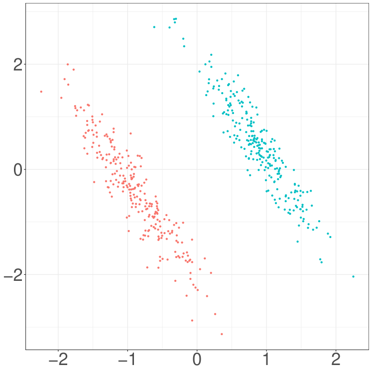
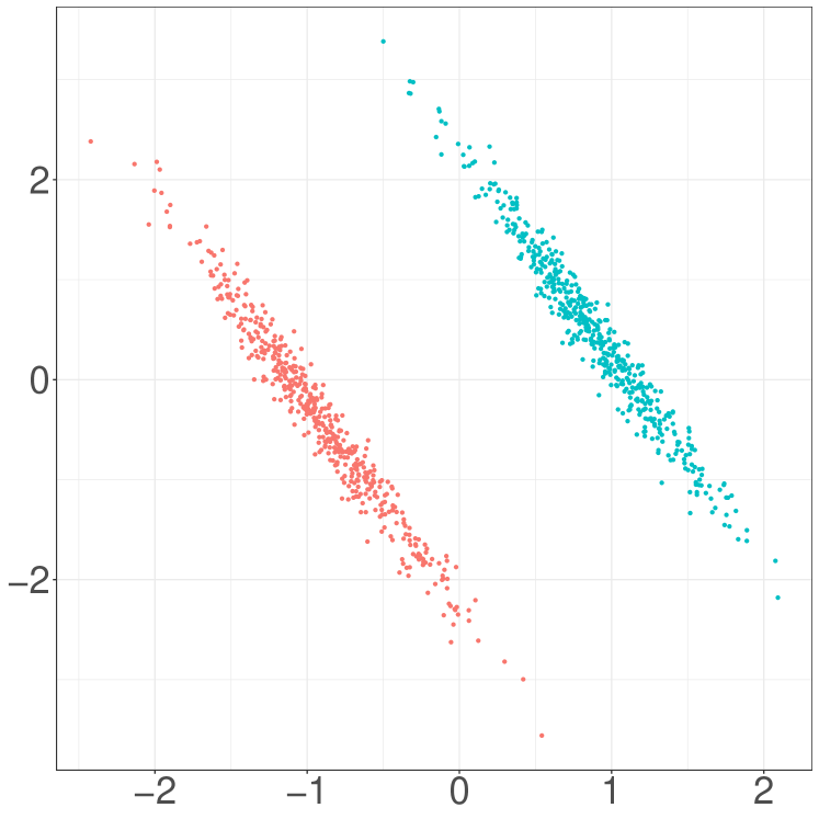
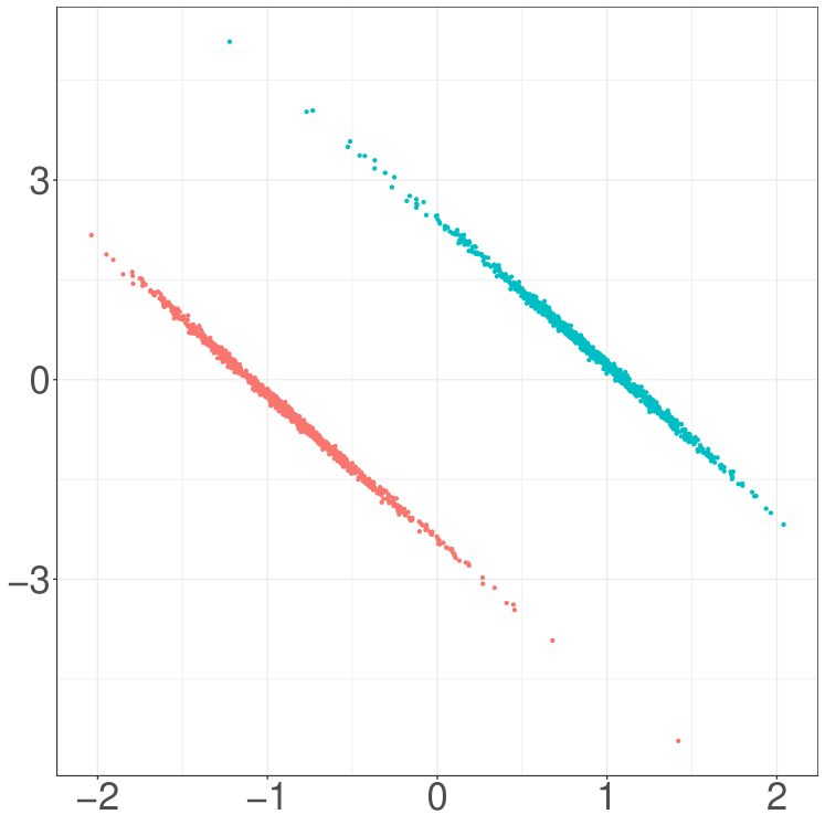
Figure 3: Scatter plot of $L(\mathcal{W})$. Set $m=1,q=2,r_{ij}=20$ and $n\in\{500,1000,2000\}$ for all subjects and features, set $|\mathcal{C}_{1}|=|\mathcal{C}_{2}|=n/2,\mu_{\mathcal{C}_{1}}\in\{5,10,50\}$ and $\mu_{\mathcal{C}_{2}}=-\mu_{\mathcal{C}_{1}}$. (a). scatter plot of $L(\mathcal{W})$ with $n=500$ and $\lVert\mu_{\mathcal{C}_{1}}-\mu_{\mathcal{C}_{2}}\rVert_{\infty}=10$. (b). scatter plot of $L(\mathcal{W})$ with $n=1000$ and $\lVert\mu_{\mathcal{C}_{1}}-\mu_{\mathcal{C}_{2}}\rVert_{\infty}=20$. (c). scatter plot of $L(\mathcal{W})$ with $n=2000$ and $\lVert\mu_{\mathcal{C}_{1}}-\mu_{\mathcal{C}_{2}}\rVert_{\infty}=100$.

Theorem 2.

(Statistical power). Suppose that $\mathcal{W}$ follows Model (1) and $w$ is a realization of $\mathcal{W}$. Suppose that the partition $\mathcal{C}(L(w))=\{\mathcal{C}_{1},\mathcal{C}_{2}\}$ ($\mathcal{C}_{1}\cup\mathcal{C}_{2}=[n]$, $\mathcal{C}_{1}\cap\mathcal{C}_{2}=\emptyset$) is the output of a clustering algorithm $\mathcal{C}(\cdot)$. Suppose that $\text{vec}(H(\mathcal{W})[i,:,:])\sim\mathcal{N}(\text{vec}(\beta_{(i)}),\Lambda)$ if the alternative hypothesis $H_{1}^{\{\mathcal{C}_{1},\mathcal{C}_{2}\}}$ holds. Then for all $\alpha\in(0,1]$, we have

$$\lim_{\lVert\mu_{\mathcal{C}_{1}}-\mu_{\mathcal{C}_{2}}\rVert_{\infty}\rightarrow\infty,n\rightarrow\infty}\mathbb{P}_{H_{1}^{\{\mathcal{C}_{1},\mathcal{C}_{2}\}}}\left(p(\mathcal{W};\mathcal{C}_{1},\mathcal{C}_{2})\leq\alpha\big{|}~{}\mathcal{C}_{1},\mathcal{C}_{2}\in\mathcal{C}(L(\mathcal{W}))\right)=1$$

if (i): $|\mathcal{C}_{1}|,|\mathcal{C}_{2}|\rightarrow\infty$ and $|\mathcal{C}_{1}|/|\mathcal{C}_{2}|\rightarrow c\in(0,1)$ as $n\rightarrow\infty$, (ii): for any $\epsilon,\delta>0$, there exists $M>0$ such that $\mathbb{P}_{H_{1}^{\{\mathcal{C}_{1},\mathcal{C}_{2}\}}}\left(\sqrt{1/|\mathcal{C}_{1}|+1/|\mathcal{C}_{2}|}\cdot s\in\mathcal{S}(\mathcal{W};\mathcal{C}_{1},\mathcal{C}_{2})\right)\geq 1-\epsilon$ for any $s>\delta$, $\lVert\mu_{\mathcal{C}_{1}}-\mu_{\mathcal{C}_{2}}\rVert_{\infty}>M$ and $n>M$. Here, the covariance function $R$ is fixed.

Proof.

See Appendix A.2. ∎

We briefly explain Assumptions (i) and (ii) in the above theorem. First, Assumption (i) implies that two clusters are asymptotically balanced as the sample size increases. Secondly, Assumption (ii) suggests that the lower bound of $\mathcal{S}(\mathcal{W};\mathcal{C}_{1},\mathcal{C}_{2})$ converges to 0 as $n$ and $\lVert\mu_{\mathcal{C}_{1}}-\mu_{\mathcal{C}_{2}}\rVert_{\infty}$ increase. Recall the geometric intuition of $\mathcal{S}(\mathcal{W};\mathcal{C}_{1},\mathcal{C}_{2})$ in Section 3.4, the lower bound of $\mathcal{S}(\mathcal{W};\mathcal{C}_{1},\mathcal{C}_{2})$ is the maximum range of “push back” under the linear operator $F(\cdot)$ that remains the same clustering outputs. Figure 3 shows the shape of two clusters becomes flatter as $n$ and $\lVert\mu_{\mathcal{C}_{1}}-\mu_{\mathcal{C}_{2}}\rVert_{\infty}$ increase. Thus, the clustering algorithm may recover $\mathcal{C}_{1},\mathcal{C}_{2}$ even if the distance of two clusters and the lower bound of $\mathcal{S}(\mathcal{W};\mathcal{C}_{1},\mathcal{C}_{2})$ tend to zero when $n$ and $\lVert\mu_{\mathcal{C}_{1}}-\mu_{\mathcal{C}_{2}}\rVert_{\infty}$ grow, namely Assumption (ii) is feasible. In addition, we intuitively explain why clusters become flatter as $n$ and $\lVert\mu_{\mathcal{C}_{1}}-\mu_{\mathcal{C}_{2}}\rVert_{\infty}$ grow: recall that $\text{vec}(L(\mathcal{W})[i,:,:])=\widehat{\Lambda}^{-\frac{1}{2}}\text{vec}(H(\mathcal{W})[i,:,:])\sim\mathcal{N}(\widehat{\Lambda}^{-\frac{1}{2}}\text{vec}(\beta_{(i)}),\widehat{\Lambda}^{-\frac{1}{2}}\Lambda\widehat{\Lambda}^{-\frac{1}{2}})$. Therefore, as $n$ and $\lVert\mu_{\mathcal{C}_{1}}-\mu_{\mathcal{C}_{2}}\rVert_{\infty}$ increase, $\widehat{\Lambda}^{-\frac{1}{2}}\Lambda\widehat{\Lambda}^{-\frac{1}{2}}$ is approximately singular and the shape of clusters becomes flatter.

5 Simulation Studies

In this section, we conduct experiments on synthetic data to evaluate the performance of the proposed procedure PSIMF. We first assess the selective type-I error to verify the consistency of PSIMF’s performance with Theorem 1. Subsequently, we examine the statistical power and explore the robustness of the proposed selective inference framework in Section 5. Due to page constraints, we provide the basic setup and discussion of the experiments in this section, while the figures of the experiments are presented in Appendix C.

Selective type-I error under a global null.

We generate a dataset containing $100$ instances following Model (1), where each instance contains $n=10000$ subjects, $m=1$ feature, and $r_{ij}=15$ time points. Specifically, for all $s\in[100]$, $i\in[n]$, and $j\in[m]$, we generate $\Omega_{i}^{(s)}=\{t_{ijk}\}_{k\in[r_{ij}]}$, where $t_{ijk}\stackrel{{\scriptstyle iid}}{{\sim}}\mathcal{U}[0,1]$ and $W_{ij}^{(s)}(t_{ijk})=Z_{ij}^{(s)}(t_{ijk})+\epsilon_{ijk}^{(s)}$, where $Z_{i}^{(s)}\sim\mathcal{MGP}(\mu_{i},R)$, $\epsilon_{ijk}^{(s)}\stackrel{{\scriptstyle iid}}{{\sim}}\mathcal{N}(0,\sigma_{j}^{2})$, and $Z_{i}^{(s)},\epsilon_{ijk}^{(s)}$ are independent. Here we set $\sigma_{j}^{2}=0.1$, $\mu_{i}=0$ and conduct the simulation for three different covariance functions:

1. Rational quadratic kernel

   $$R(x,y)=\left(1+\frac{(x-y)^{2}}{\ell^{2}}\right)^{-1/2};$$

2. Periodic kernel

   $$R(x,y)=e^{-{8\sin^{2}(2\pi|x-y|)}};$$

3. Truncated local periodic kernel

   $$R(x,y)=\mathbbm{1}_{\{1/3<|x-y|<2/3\}}\cdot e^{-8\sin^{2}(2\pi|x-y|)}e^{-2(x-y)^{2}}+\mathbbm{1}_{\{|x-y|\leq 1/3~{}\text{or}~{}|x-y|\geq 2/3\}}\cdot 0.01.$$

Next, we set the basis functions $\{\phi_{s}\}_{s\in[q]}$ as the eigenfunctions of the Gaussian RBF (Radial Basis Function) kernel $R(x,y)=e^{-\frac{\rho}{1-\rho^{2}}(x-y)^{2}}$, where $\rho\in(0,1)$. By the Mercer expansion (Fasshauer and McCourt, 2012), the $i$-th eigenfunction of $R(x,y)$ is

$$\phi_{i}(x)=\frac{1}{\sqrt{N_{i}}}H_{i}(x)e^{-\frac{\rho}{1+\rho}x^{2}},$$ (23)

where $N_{i}=2^{i}i!\sqrt{\frac{1-\rho}{1+\rho}}$ and $H_{i}(x)$ is the $i$-th order physicist’s Hermite polynomial. In this experiment, we set $\rho=0.99$ and set the truncation number $q$ to be $3$, i.e., we use the first three eigenfunctions to conduct the low-dimensional embedding.

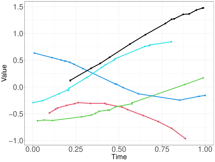
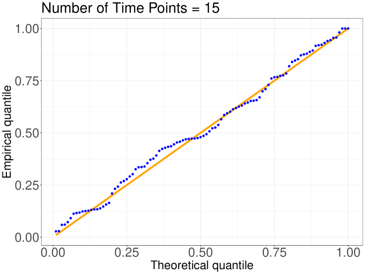
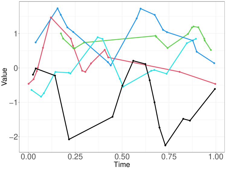
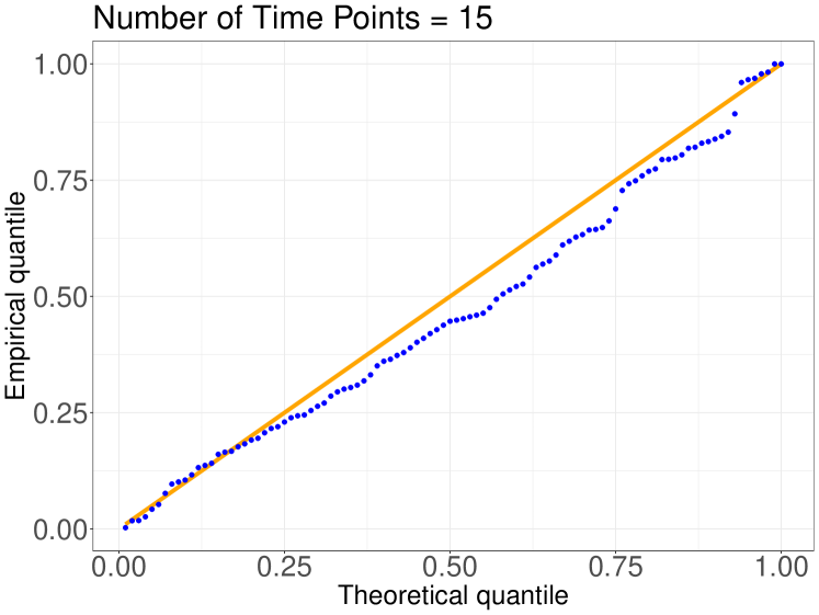
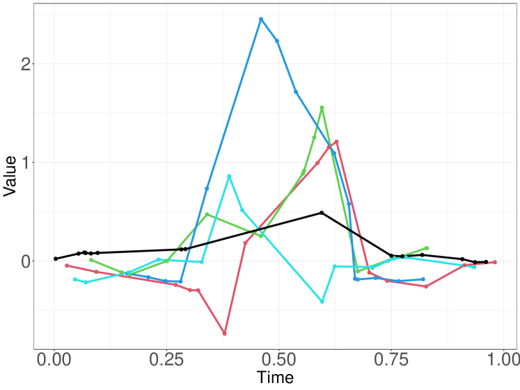
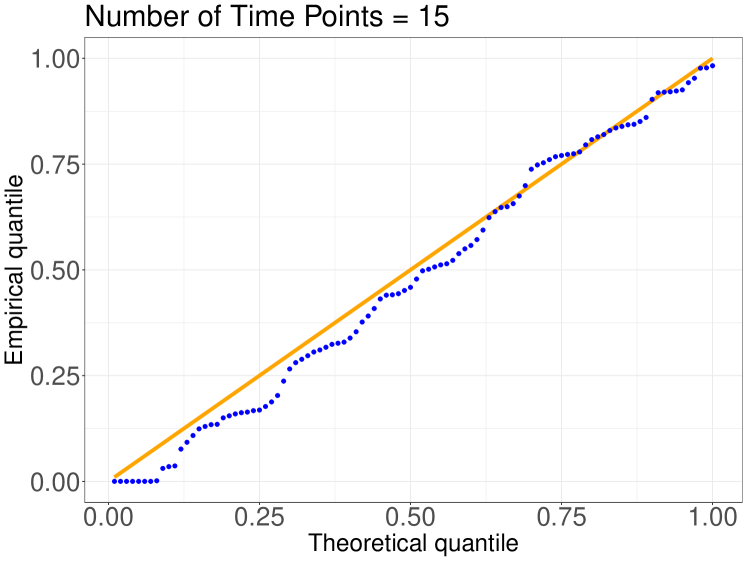
Figure 5: Left column: Records of the first feature and the first 5 subjects for the dataset generated with $15$ time points. Right column: Quantile plots of the selective $p$-value for the corresponding kernel with $100$ generated datasets, where (b) is the result of RQ Kernel, (d) is the result of PE Kernel, and (f) is the result of LPE Kernel.

Now, we apply the proposed selective inference framework to the generated datasets. Figure 5 displays quantile plots of the selective $p$-values for datasets corresponding to the three kernels above. The plots demonstrate that the selective $p$-values approximately follow a uniform distribution under the global null hypothesis, thereby validating the statement of Theorem 1.

Statistical power.

Next, we present numerical results to verify Theorem 2. Specifically, we generate datasets following Model (1) under the alternative hypothesis and compute the corresponding statistical power. We compute the selective $p$-value for datasets generated with varying cluster means $\lVert\mu_{\mathcal{C}_{1}}-\mu_{\mathcal{C}_{2}}\rVert_{\infty}$ and sample sizes $n$.

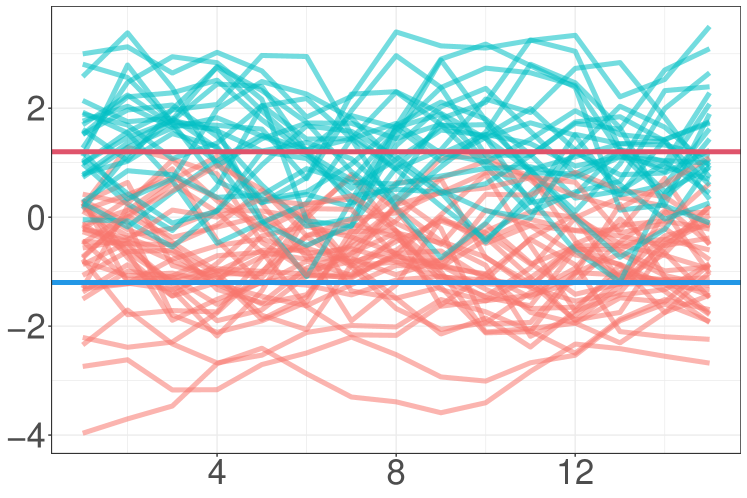
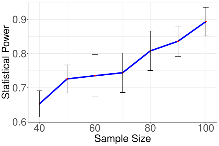
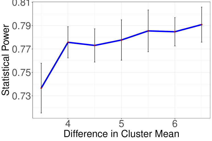
Figure 6: (a): Example of the dataset generated under $H_{1}^{\{\mathcal{C}_{1},\mathcal{C}_{2}\}}$ with $15$ time points and sample size $m=80$, where population means are $\mu_{i}(\cdot)=1.1$ for $i\leq 50$ and $\mu_{i}(\cdot)=-1.1$ for $i>50$. (b): Statistical power with sample size $m\in\{40,50,\cdots,100\}$, where population means are $\mu_{i}(\cdot)=10$ for $i\leq m/2$ and $\mu_{i}(\cdot)=-10$ for $i>m/2$. (c): Statistical power with sample size $m=80$ and population means $\mu_{i}(\cdot)=k$ for $i\leq m/2$ and $\mu_{i}(\cdot)=-k$ for $i>m/2$, where $k\in\{3.5,4,\cdots,6.5\}$.

We set the sample size $n=10k$ for $k\in\{4,\ldots,10\}$. We fix $m=1$ and set $r_{ij}=15$, $\sigma_{j}^{2}=0.1$ for all $i\in[n],j\in[m]$. For each sample size $n$, we generate a dataset containing $n$ subjects following the alternative hypothesis: $\mu_{i}(\cdot)=-10$ for $i\leq m/2$ and $\mu_{i}(\cdot)=10$ for $i>m/2$. We use the same basis as in (23) with the parameter $q=3$ to conduct the low-dimensional embedding. Figure 6 presents the statistical power with a fixed mean difference and increasing sample sizes, showing that the statistical power increases as the sample size increases.

To investigate the statistical power for different cluster means, we fix the sample size at $n=80$ and the other parameters remaining the same as in the previous paragraph. For each $k\in\{3.5,4,4.5,5,5.5,6,6.5\}$, we generate a dataset with $n$ records with population means $\mu_{i}(\cdot)=k$ for $i\leq n/2$ and $\mu_{i}(\cdot)=-k$ for $i>n/2$. Figure 6 presents the statistical power with the same sample size and the increasing difference between cluster means, it shows that the statistical power increases as the difference between cluster means increases.

Empirical robustness analysis.

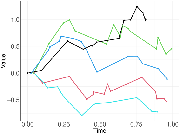
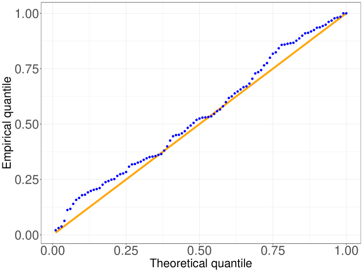
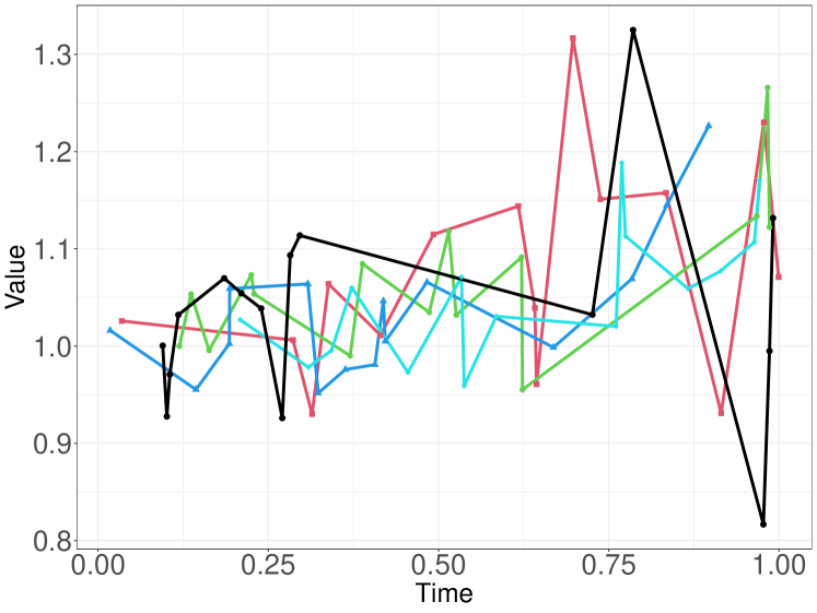
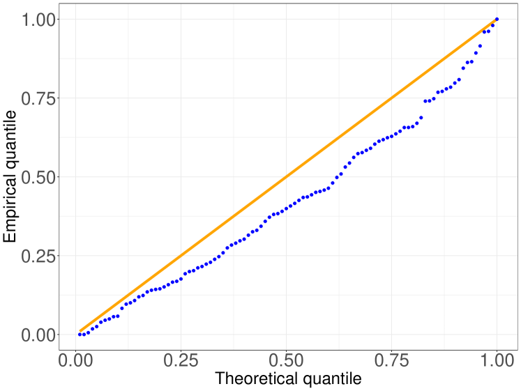
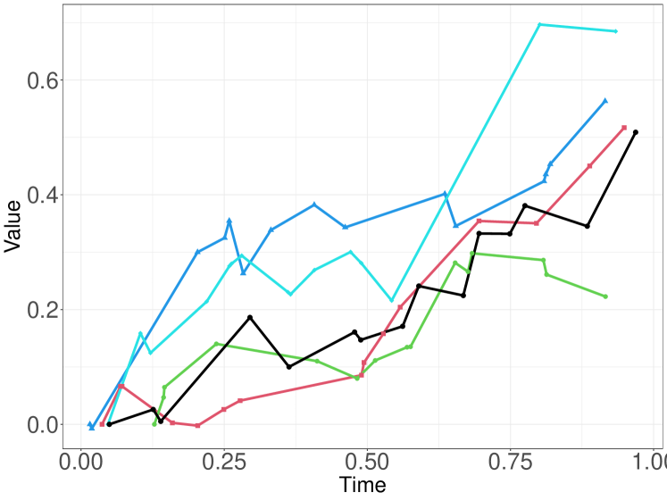
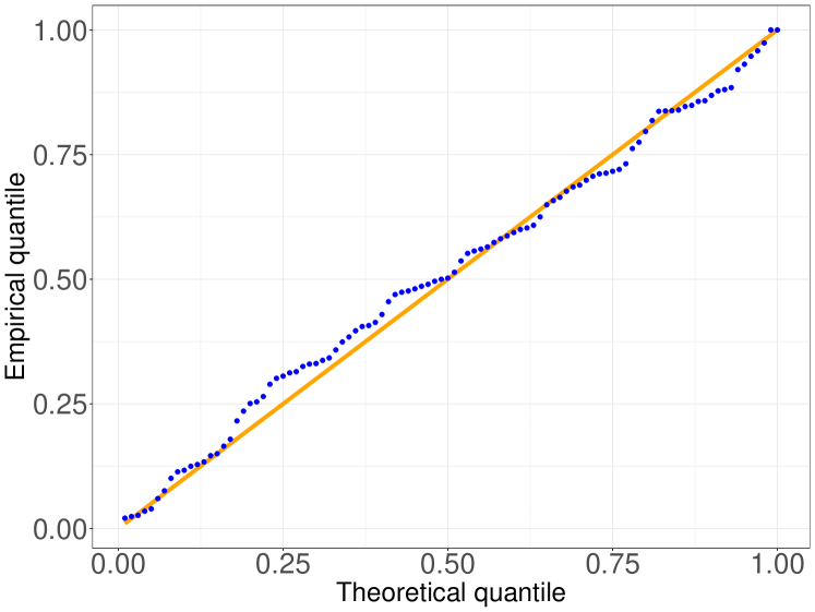
Figure 7: Left column: Records of the first feature of the first 5 subjects for the dataset generated with $15$. Right column: quantile plots of the selective $p$-value. (a): Each record is generated independently under the Wiener process. (c): Each record is generated independently under the exponential Brownian motion. (e): Each record is generated independently under the OU process.

We consider three misspecification cases and compute the selective $p$-value under a global null: Wiener process (Figure 7), exponential Brownian motion (Figure 7), and Ornstein–Uhlenbeck (OU) process (Figure 7). We also present the QQ-plot of the selective $p$-value in Appendix C.

6 Phenotyping of AKI based on EHR

Now we present a real-data application of our selective inference framework. Acute Kidney Injury (AKI) is a common clinical syndrome characterized by a complex treatment process and high mortality rates. The pathology of AKI exhibits a high degree of heterogeneity, posing significant challenges to the formulation of treatment plans. Consequently, identifying new AKI subtypes is crucial for improving patient outcomes. The severity of the disease in AKI patients tends to vary over time, making the problem of hypothesis testing for functional disease subtypes of significant practical importance.

We specifically focus on the MIMIC-IV EHR dataset from PhysioNet (Johnson et al., 2020, 2023; Goldberger et al., 2000), which contains de-identified medical data from patients admitted to the Intensive Care Units (ICU) at Beth Israel Deaconess Medical Center from 2008 to 2019. The database provides a variety of medical data, including vital signs, medications, laboratory measurements, diagnostic codes, and hospital length of stay. This dataset is rich in individual patient-level information and is freely accessible, making it feasible for clinical research worldwide.

We focus on data from adult patients with AKI admitted to the ICU. We identify patients with ICD codes with explanations including “acute kidney failure.” Then we preprocess the data similarly to the framework provided by (Song et al., 2020), excluding patients at or before admission with 1) End Stage Renal Disease, 2) Burns, and 3) Renal Dialysis. Subsequently, according to the clinical practice guidelines for Acute Kidney Injury designated by Kidney Disease Improving Global Outcomes (KDIGO):

• Stage 1: Serum creatinine (SCr) value rises to 1.5-1.9 times the baseline value within 7 days or SCr value increases $\geq$ 0.3 mg/dl within 48 hours.

• Stage 2: SCr value rises to 2.0-2.9 times the baseline value within 7 days.

• Stage 3: meets at least one of the following two conditions:

  • SCr value rises to 3 times the baseline value or more within 7 days;

  • increase in SCr value to $\geq$ 4.0 mg/dl within 48 hours.

We further divide Stage 3 into two subclasses: S3-1, where there is an increase in SCr value to $\geq$ 4.0 mg/dl within 48 hours; and S3-2, where the SCr value increases to three times the baseline or more within 7 days without meeting the conditions of S3-1. The specific shape of this longitudinal data is shown in Figure 4. For consistency in definition, we selected data from the first seven days as our study subjects. We then used hierarchical clustering based on squared Euclidean distance to cluster each category combination, specifying the number of clusters as 2. In this clustering scenario, we compared the $p$-values under two distinct test methods: PSIMF, performing the post-clustering hypothesis test (2), and the Wald test.

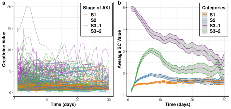
Figure 4: a. Real trajectories for 100 randomly selected patients from each category. b. Trajectories (Mean $\pm$ $1.96\times$ standard deviation/$\sqrt{\text{sample size}}$) of the four AKI subtypes.

Included data	S1	S2	S3-1	S3-2	(S1, S3-1)	(S1, S3-2)	(S3-1, S3-2)
PSIMF $p$-value	0.2070	0.4504	0.5324	0.9033	0.0095	0.0254	0.5455
Wald $p$-value	$<10^{-307}$	$<10^{-307}$	$<10^{-307}$	$<10^{-307}$	$<10^{-307}$	$<10^{-307}$	$<10^{-307}$

Table 1: Comparison of $p$-values under different clustering scenarios.

As indicated in Table 1, when the input data comprises only one cohort of patients (S1, S2, S3-1, or S3-2), the $p$-values produced by PSIMF are relatively high, whereas those from the Wald test are significantly lower. Our approach appropriately refrains from rejecting the null hypothesis, unlike the Wald test. This suggests that PSIMF effectively recognizes the inherent homogeneity among these subtypes.

When the input data includes patients from different AKI stages, the $p$-value for the combination of S1 and S3-1 is low, correctly indicating the heterogeneity of this combined class. Clinically, given the definitions of AKI, S1 and S3-1 exhibit significant differences in distribution and mean, justifying the rejection of the null hypothesis. Similarly, the $p$-value for the combination of S1 and S3-2 is also low. We recognize that these two categories are not adjacent in the clinical staging of AKI—with S1 involving an SCr rise to 1.5-1.9 times the baseline within 7 days, and S3-2 defined by an SCr increase to three times the baseline or more. Therefore, the significant results under PSIMF  are justified due to the non-adjacent staging definitions.

Lastly, the $p$-value produced by PSIMF for the combination of S3-1 and S3-2 is relatively high, suggesting that S3-1 and S3-2 likely represent the same subtype. This is clinically plausible, as both S3-1 and S3-2 are categorized under Stage-3 AKI and are not sufficiently distinct to warrant classification into separate subtypes.

7 Discussions

This paper focuses on the post-clustering inference problem for functional data. We establish a selective inference framework and propose a selective $p$-value for functional data that reduces the selective bias induced by the clustering algorithm. Our theoretical results show that the proposed method controls the selective type-I error and statistical power when there are sufficient time records and sufficient subjects. We use numerical simulation to verify our theory and further apply the method to the phenotyping of Acute Kidney Injury (AKI), in which the selective $p$-value between different stages matches the medical consensus.

Our work opens up several avenues for future research. In this paper, we primarily focus on scenarios where $t_{ijk}\sim\mathcal{U}[0,1]$. However, in real-world applications, time records may be more concentrated during certain periods, potentially invalidating this assumption. A valuable direction for future research would be to extend our theoretical results to accommodate a broader class of distributions for $t_{ijk}$. Additionally, our analysis of selective type-I error and statistical power currently relies on asymptotic approximations, using the limiting distribution of $H(\mathcal{W})$ with an infinite number of time records. Addressing the challenge of deriving finite-sample results for selective type-I error and statistical power remains an open problem and an important next step.

In addition, we study the setting where clustering algorithms output two clusters, and it would be interesting to extend the selective inference framework to the setting of multiple clusters. For this problem, a key challenge would be estimating the unknown kernel function with multiple clusters. To elaborate, in Section 3.2, we leverage all the data within two clusters and consider the sample covariance estimator. When there are multiple clusters, the transformed data $\text{vec}(L(\mathcal{W})[i,:,:])$ within each cluster follows a truncated multivariate normal distribution. Therefore, combining two clusters and leveraging the sample covariance estimator would be biased.

Furthermore, the proposed method necessitates that the clustering algorithm $\mathcal{C}(\cdot)$ be applicable to a collection of matrix data ${L(w)[i,:,:]}_{i\in[n]}$. Extending our framework to accommodate a broader class of clustering algorithms is another interesting area for future research.

Appendix A Proof of Main Theorems

A.1 Proof of Theorem 1

Suppose $w$ is a realization of (1) and $\mathcal{C}_{1},\mathcal{C}_{2}$ is the partition obtain by a clustering algorithm based on $L(w)$. For any $\alpha\in[0,1]$, we consider the following conditional probability:

$$\mathbb{P}_{H_{0}^{\{\mathcal{C}_{1},\mathcal{C}_{2}\}}}\bigg{(}p(\mathcal{W};\mathcal{C}_{1},\mathcal{C}_{2})\leq\alpha\bigg{|} \mathcal{C}_{1},\mathcal{C}_{2}\in\mathcal{C}(L(\mathcal{W})),\pi^{\perp}_{\nu(\mathcal{C}_{1},\mathcal{C}_{2})}\times_{1}L(\mathcal{W})=\pi^{\perp}_{\nu(\mathcal{C}_{1},\mathcal{C}_{2})}\times_{1}L(w),$$ (24)

$$\text{dir}(\overline{L(\mathcal{W})}_{\mathcal{C}_{1}}-\overline{L(\mathcal{W})}_{\mathcal{C}_{2}})=\text{dir}(\overline{L(w)}_{\mathcal{C}_{1}}-\overline{L(w)}_{\mathcal{C}_{2}})\bigg{)}.$$

Given the partition $\mathcal{C}_{1},\mathcal{C}_{2}$, for any $\mathcal{W}$ follows Model (1) and satisfies $\mathcal{C}_{1},\mathcal{C}_{2}\in\mathcal{C}(L(\mathcal{W}))$, (19) implies that

$$p(\mathcal{W};\mathcal{C}_{1},\mathcal{C}_{2})=1-\mathbb{F}\left(\lVert\overline{L(\mathcal{W})}_{\mathcal{C}_{1}}-\overline{L(\mathcal{W})}_{\mathcal{C}_{2}}\rVert_{F};\sqrt{\frac{1}{|\mathcal{C}_{1}|}+\frac{1}{|\mathcal{C}_{2}|}},\mathcal{S}(\mathcal{W};\mathcal{C}_{1},\mathcal{C}_{2})\right).$$

Therefore, we rewrite (24) as follows:

$$\mathbb{P}_{H_{0}^{\{\mathcal{C}_{1},\mathcal{C}_{2}\}}}\bigg{(} 1-\mathbb{F}\left(\lVert\overline{L(\mathcal{W})}_{\mathcal{C}_{1}}-\overline{L(\mathcal{W})}_{\mathcal{C}_{2}}\rVert_{F};\sqrt{\frac{1}{|\mathcal{C}_{1}|}+\frac{1}{|\mathcal{C}_{2}|}},\mathcal{S}(\mathcal{W};\mathcal{C}_{1},\mathcal{C}_{2})\right)\leq\alpha\bigg{|}\mathcal{C}_{1},\mathcal{C}_{2}\in\mathcal{C}(L(\mathcal{W})),$$ (25)

$$\pi^{\perp}_{\nu(\mathcal{C}_{1},\mathcal{C}_{2})}\times_{1}L(\mathcal{W})=\pi^{\perp}_{\nu(\mathcal{C}_{1},\mathcal{C}_{2})}\times_{1}L(w),\text{dir}(\overline{L(\mathcal{W})}_{\mathcal{C}_{1}}-\overline{L(\mathcal{W})}_{\mathcal{C}_{2}})=\text{dir}(\overline{L(w)}_{\mathcal{C}_{1}}-\overline{L(w)}_{\mathcal{C}_{2}})\bigg{)}.$$

Under the conditions $\pi^{\perp}_{\nu(\mathcal{C}_{1},\mathcal{C}_{2})}\times_{1}L(\mathcal{W})=\pi^{\perp}_{\nu(\mathcal{C}_{1},\mathcal{C}_{2})}\times_{1}L(w),\text{dir}(\overline{L(\mathcal{W})}_{\mathcal{C}_{1}}-\overline{L(\mathcal{W})}_{\mathcal{C}_{2}})=\text{dir}(\overline{L(w)}_{\mathcal{C}_{1}}-\overline{L(w)}_{\mathcal{C}_{2}})$, the truncation sets $\mathcal{S}(\mathcal{W};\mathcal{C}_{1},\mathcal{C}_{2})$ and $\mathcal{S}(w;\mathcal{C}_{1},\mathcal{C}_{2})$ are equivalent:

$$\mathcal{S} (\mathcal{W};\mathcal{C}_{1},\mathcal{C}_{2})$$

$$=\left\{\varphi\geq 0:\mathcal{C}_{1},\mathcal{C}_{2}\in\mathcal{C}\left(\pi^{\perp}_{\nu(\mathcal{C}_{1},\mathcal{C}_{2})}\times_{1}L(\mathcal{W})+\left[\frac{\varphi}{\frac{1}{|\mathcal{C}_{1}|}+\frac{1}{|\mathcal{C}_{2}|}}\right]\nu(\mathcal{C}_{1},\mathcal{C}_{2})\times_{1}\text{dir}(\overline{L(\mathcal{W})}_{\mathcal{C}_{1}}-\overline{L(\mathcal{W})}_{\mathcal{C}_{2}})^{\top}\right)\right\}$$

$$=\left\{\varphi\geq 0:\mathcal{C}_{1},\mathcal{C}_{2}\in\mathcal{C}\left(\pi^{\perp}_{\nu(\mathcal{C}_{1},\mathcal{C}_{2})}\times_{1}L(w)+\left[\frac{\varphi}{\frac{1}{|\mathcal{C}_{1}|}+\frac{1}{|\mathcal{C}_{2}|}}\right]\nu(\mathcal{C}_{1},\mathcal{C}_{2})\times_{1}\text{dir}(\overline{L(w)}_{\mathcal{C}_{1}}-\overline{L(w)}_{\mathcal{C}_{2}})^{\top}\right)\right\}$$

$$=\mathcal{S}(w;\mathcal{C}_{1},\mathcal{C}_{2}).$$

Note that the random variable $\lVert\overline{L(\mathcal{W})}_{\mathcal{C}_{1}}-\overline{L(\mathcal{W})}_{\mathcal{C}_{2}}\rVert_{F}$ is independent of $\pi^{\perp}_{\nu(\mathcal{C}_{1},\mathcal{C}_{2})}\times_{1}L(\mathcal{W})$ and $\text{dir}(\overline{L(w)}_{\mathcal{C}_{1}}-\overline{L(w)}_{\mathcal{C}_{2}})$ (we refer readers to Appendix B.3 for the proof). Therefore, the conditional probability (25) can be rewritten as follows

$$\mathbb{P}_{H_{0}^{\{\mathcal{C}_{1},\mathcal{C}_{2}\}}}\bigg{(}1-\mathbb{F}\left(\lVert\overline{L(\mathcal{W})}_{\mathcal{C}_{1}}-\overline{L(\mathcal{W})}_{\mathcal{C}_{2}}\rVert_{F};\sqrt{\frac{1}{|\mathcal{C}_{1}|}+\frac{1}{|\mathcal{C}_{2}|}},\mathcal{S}(w;\mathcal{C}_{1},\mathcal{C}_{2})\right)\leq\alpha\bigg{|}$$ (26)

$$\quad\mathcal{C}_{1},\mathcal{C}_{2}\in\mathcal{C}\bigg{(}\pi^{\perp}_{\nu(\mathcal{C}_{1},\mathcal{C}_{2})}\times_{1}L(w)+\left[\frac{\lVert\overline{L(\mathcal{W})}_{\mathcal{C}_{1}}-\overline{L(\mathcal{W})}_{\mathcal{C}_{2}}\rVert_{F}}{1/|\mathcal{C}_{1}|+1/|\mathcal{C}_{2}|}\right]\nu(\mathcal{C}_{1},\mathcal{C}_{2})\times_{1}\text{dir}(\overline{L(w)}_{\mathcal{C}_{1}}-\overline{L(w)}_{\mathcal{C}_{2}})^{\top}\bigg{)},$$

$$\quad\pi^{\perp}_{\nu(\mathcal{C}_{1},\mathcal{C}_{2})}\times_{1}L(\mathcal{W})=\pi^{\perp}_{\nu(\mathcal{C}_{1},\mathcal{C}_{2})}\times_{1}L(w),\text{dir}(\overline{L(\mathcal{W})}_{\mathcal{C}_{1}}-\overline{L(\mathcal{W})}_{\mathcal{C}_{2}})=\text{dir}(\overline{L(w)}_{\mathcal{C}_{1}}-\overline{L(w)}_{\mathcal{C}_{2}})\bigg{)}$$

$$= \mathbb{P}_{H_{0}^{\{\mathcal{C}_{1},\mathcal{C}_{2}\}}}\bigg{(}1-\mathbb{F}\left(\lVert\overline{L(\mathcal{W})}_{\mathcal{C}_{1}}-\overline{L(\mathcal{W})}_{\mathcal{C}_{2}}\rVert_{F};\sqrt{\frac{1}{|\mathcal{C}_{1}|}+\frac{1}{|\mathcal{C}_{2}|}},\mathcal{S}(w;\mathcal{C}_{1},\mathcal{C}_{2})\right)\leq\alpha\bigg{|}$$

$$\quad\mathcal{C}_{1},\mathcal{C}_{2}\in\mathcal{C}\bigg{(}\pi^{\perp}_{\nu(\mathcal{C}_{1},\mathcal{C}_{2})}\times_{1}L(w)+\left[\frac{\lVert\overline{L(\mathcal{W})}_{\mathcal{C}_{1}}-\overline{L(\mathcal{W})}_{\mathcal{C}_{2}}\rVert_{F}}{1/|\mathcal{C}_{1}|+1/|\mathcal{C}_{2}|}\right]\nu(\mathcal{C}_{1},\mathcal{C}_{2})\times_{1}\text{dir}(\overline{L(w)}_{\mathcal{C}_{1}}-\overline{L(w)}_{\mathcal{C}_{2}})^{\top}\bigg{)}\bigg{)}$$

$$= \mathbb{P}_{H_{0}^{\{\mathcal{C}_{1},\mathcal{C}_{2}\}}}\bigg{(}1-\mathbb{F}\left(\lVert\overline{L(\mathcal{W})}_{\mathcal{C}_{1}}-\overline{L(\mathcal{W})}_{\mathcal{C}_{2}}\rVert_{F};\sqrt{\frac{1}{|\mathcal{C}_{1}|}+\frac{1}{|\mathcal{C}_{2}|}},\mathcal{S}(w;\mathcal{C}_{1},\mathcal{C}_{2})\right)\leq\alpha\bigg{|}$$

$$\quad\lVert\overline{L(\mathcal{W})}_{\mathcal{C}_{1}}-\overline{L(\mathcal{W})}_{\mathcal{C}_{2}}\rVert_{F}\in\mathcal{S}(w;\mathcal{C}_{1},\mathcal{C}_{2})\bigg{)}.$$

Plugging (26) into (24), we have

$$\mathbb{P}_{H_{0}^{\{\mathcal{C}_{1},\mathcal{C}_{2}\}}}\bigg{(}p(\mathcal{W};\mathcal{C}_{1},\mathcal{C}_{2})\leq\alpha\bigg{|}\mathcal{C}_{1},\mathcal{C}_{2}\in\mathcal{C}(L(\mathcal{W})),\pi^{\perp}_{\nu(\mathcal{C}_{1},\mathcal{C}_{2})}\times_{1}L(\mathcal{W})=\pi^{\perp}_{\nu(\mathcal{C}_{1},\mathcal{C}_{2})}\times_{1}L(w),$$ (27)

$$\quad\text{dir}(\overline{L(\mathcal{W})}_{\mathcal{C}_{1}}-\overline{L(\mathcal{W})}_{\mathcal{C}_{2}})=\text{dir}(\overline{L(w)}_{\mathcal{C}_{1}}-\overline{L(w)}_{\mathcal{C}_{2}})\bigg{)}$$

$$= \mathbb{P}_{H_{0}^{\{\mathcal{C}_{1},\mathcal{C}_{2}\}}}\bigg{(}1-\mathbb{F}\left(\lVert\overline{L(\mathcal{W})}_{\mathcal{C}_{1}}-\overline{L(\mathcal{W})}_{\mathcal{C}_{2}}\rVert_{F};\sqrt{\frac{1}{|\mathcal{C}_{1}|}+\frac{1}{|\mathcal{C}_{2}|}},\mathcal{S}(w;\mathcal{C}_{1},\mathcal{C}_{2})\right)\leq\alpha\bigg{|}$$

$$\quad\lVert\overline{L(\mathcal{W})}_{\mathcal{C}_{1}}-\overline{L(\mathcal{W})}_{\mathcal{C}_{2}}\rVert_{F}\in\mathcal{S}(w;\mathcal{C}_{1},\mathcal{C}_{2})\bigg{)}=\alpha.$$

Now we use (27) to compute the selective $p$-value. By the law of iterated expectation, we rewrite the selective type-I error as follows:

$$\mathbb{P}_{H_{0}^{\{\mathcal{C}_{1},\mathcal{C}_{2}\}}}\left(p(\mathcal{W};\mathcal{C}_{1},\mathcal{C}_{2})\leq\alpha\big{|}~{}\mathcal{C}_{1},\mathcal{C}_{2}\in\mathcal{C}(L(\mathcal{W}))\right)=\mathbb{E}_{H_{0}^{\{\mathcal{C}_{1},\mathcal{C}_{2}\}}}\left(\mathbbm{1}_{p(\mathcal{W};\mathcal{C}_{1},\mathcal{C}_{2})\leq\alpha}\big{|}~{}\mathcal{C}_{1},\mathcal{C}_{2}\in\mathcal{C}(L(\mathcal{W}))\right)$$

$$=\mathbb{E}_{H_{0}^{\{\mathcal{C}_{1},\mathcal{C}_{2}\}}}\bigg{(}\mathbb{E}\big{[}\mathbbm{1}_{p(\mathcal{W};\mathcal{C}_{1},\mathcal{C}_{2})\leq\alpha}\big{|}\mathcal{C}_{1},\mathcal{C}_{2}\in\mathcal{C}(L(\mathcal{W})),\pi^{\perp}_{\nu(\mathcal{C}_{1},\mathcal{C}_{2})}\times_{1}L(\mathcal{W})=\pi^{\perp}_{\nu(\mathcal{C}_{1},\mathcal{C}_{2})}\times_{1}L(w),$$

$$\quad\quad\quad\quad\quad\quad\text{dir}(\overline{L(\mathcal{W})}_{\mathcal{C}_{1}}-\overline{L(\mathcal{W})}_{\mathcal{C}_{2}})=\text{dir}(\overline{L(w)}_{\mathcal{C}_{1}}-\overline{L(w)}_{\mathcal{C}_{2}})\big{]}\big{|}~{}\mathcal{C}_{1},\mathcal{C}_{2}\in\mathcal{C}(L(\mathcal{W}))\bigg{)}.$$

Plugging in (27), we obtain

$$\mathbb{P}_{H_{0}^{\{\mathcal{C}_{1},\mathcal{C}_{2}\}}}\left(p(\mathcal{W};\mathcal{C}_{1},\mathcal{C}_{2})\leq\alpha\big{|}~{}\mathcal{C}_{1},\mathcal{C}_{2}\in\mathcal{C}(L(\mathcal{W}))\right)=\mathbb{E}_{H_{0}^{\{\mathcal{C}_{1},\mathcal{C}_{2}\}}}\bigg{(}\alpha\big{|}~{}\mathcal{C}_{1},\mathcal{C}_{2}\in\mathcal{C}(L(\mathcal{W}))\bigg{)}=\alpha.$$

A.2 Proof of Theorem 2

Plug in (19), we have

$$\mathbb{P}_{H_{1}^{\{\mathcal{C}_{1},\mathcal{C}_{2}\}}}\left(p(\mathcal{W};\mathcal{C}_{1},\mathcal{C}_{2})\leq\alpha\big{|}~{}\mathcal{C}_{1},\mathcal{C}_{2}\in\mathcal{C}(L(\mathcal{W}))\right)$$ (28)

$$= \mathbb{P}_{H_{1}^{\{\mathcal{C}_{1},\mathcal{C}_{2}\}}}\Bigg{(}1-\mathbb{F}\left(\lVert\overline{L(\mathcal{W})}_{\mathcal{C}_{1}}-\overline{L(\mathcal{W})}_{\mathcal{C}_{2}}\rVert_{F};\sqrt{\frac{1}{|\mathcal{C}_{1}|}+\frac{1}{|\mathcal{C}_{2}|}},\mathcal{S}(\mathcal{W};\mathcal{C}_{1},\mathcal{C}_{2})\right)\leq\alpha$$

$$\quad\quad\big{|}~{}\mathcal{C}_{1},\mathcal{C}_{2}\in\mathcal{C}(L(\mathcal{W}))\Bigg{)}.$$

We rewrite the survival function $\mathbb{F}(\cdot)$ as follows:

$$\begin{split}&\mathbb{F}\left(\lVert\overline{L(\mathcal{W})}_{\mathcal{C}_{1}}-\overline{L(\mathcal{W})}_{\mathcal{C}_{2}}\rVert_{F};\sqrt{\frac{1}{|\mathcal{C}_{1}|}+\frac{1}{|\mathcal{C}_{2}|}},\mathcal{S}(\mathcal{W};\mathcal{C}_{1},\mathcal{C}_{2})\right)\\ =&\mathbb{P}\left(\varphi\leq\lVert\overline{L(\mathcal{W})}_{\mathcal{C}_{1}}-\overline{L(\mathcal{W})}_{\mathcal{C}_{2}}\rVert_{F}\big{|}\varphi\in\mathcal{S}(\mathcal{W};\mathcal{C}_{1},\mathcal{C}_{2})\right),\end{split}$$

where $\varphi$ follows the distribution $\sqrt{1/|\mathcal{C}_{1}|+1/|\mathcal{C}_{2}|}\cdot\chi_{mq}$. Using the fact that $\mathbb{P}(A|B)\geq\mathbb{P}(A)-\mathbb{P}(B^{c})$, we have

$$\mathbb{P}_{H_{1}^{\{\mathcal{C}_{1},\mathcal{C}_{2}\}}}\left(p(\mathcal{W};\mathcal{C}_{1},\mathcal{C}_{2})\leq\alpha\big{|}~{}\mathcal{C}_{1},\mathcal{C}_{2}\in\mathcal{C}(L(\mathcal{W}))\right)$$ (29)

$$\leq \mathbb{P}_{H_{1}^{\{\mathcal{C}_{1},\mathcal{C}_{2}\}}}\left(1-\mathbb{F}\left(\lVert\overline{L(\mathcal{W})}_{\mathcal{C}_{1}}-\overline{L(\mathcal{W})}_{\mathcal{C}_{2}}\rVert_{F};\sqrt{\frac{1}{|\mathcal{C}_{1}|}+\frac{1}{|\mathcal{C}_{2}|}},\mathcal{S}(\mathcal{W};\mathcal{C}_{1},\mathcal{C}_{2})\right)\leq\alpha\right)$$

$$-\mathbb{P}_{H_{1}^{\{\mathcal{C}_{1},\mathcal{C}_{2}\}}}\left(\mathcal{C}_{1},\mathcal{C}_{2}\notin\mathcal{C}(L(\mathcal{W}))\right)$$

$$= \mathbb{P}_{H_{1}^{\{\mathcal{C}_{1},\mathcal{C}_{2}\}}}\left(\mathbb{P}\left(\varphi\leq\lVert\overline{L(\mathcal{W})}_{\mathcal{C}_{1}}-\overline{L(\mathcal{W})}_{\mathcal{C}_{2}}\rVert_{F}\big{|}\varphi\in\mathcal{S}(\mathcal{W};\mathcal{C}_{1},\mathcal{C}_{2})\right)\geq 1-\alpha\right)$$

$$-\mathbb{P}_{H_{1}^{\{\mathcal{C}_{1},\mathcal{C}_{2}\}}}\left(\mathcal{C}_{1},\mathcal{C}_{2}\notin\mathcal{C}(L(\mathcal{W}))\right).$$

Following assumption (ii), we obtain that

$$\lim_{\lVert\mu_{\mathcal{C}_{1}}-\mu_{\mathcal{C}_{2}}\rVert_{\infty}\rightarrow\infty,n\rightarrow\infty}\mathbb{P}_{H_{1}^{\{\mathcal{C}_{1},\mathcal{C}_{2}\}}}\left(\mathcal{C}_{1},\mathcal{C}_{2}\notin\mathcal{C}(L(\mathcal{W}))\right)=0.$$ (30)

To derive the bound for

$$\mathbb{P}_{H_{1}^{\{\mathcal{C}_{1},\mathcal{C}_{2}\}}}\left(\mathbb{P}\left(\varphi\leq\lVert\overline{L(\mathcal{W})}_{\mathcal{C}_{1}}-\overline{L(\mathcal{W})}_{\mathcal{C}_{2}}\rVert_{F}\big{|}\varphi\in\mathcal{S}(\mathcal{W};\mathcal{C}_{1},\mathcal{C}_{2})\right)\geq 1-\alpha\right),$$

we leverage the inequality $\mathbb{P}(A|B)\geq\mathbb{P}(A)-\mathbb{P}(B^{c})$ again and obtain

$$\mathbb{P}_{H_{1}^{\{\mathcal{C}_{1},\mathcal{C}_{2}\}}}\left(\mathbb{P}\left(\varphi\leq\lVert\overline{L(\mathcal{W})}_{\mathcal{C}_{1}}-\overline{L(\mathcal{W})}_{\mathcal{C}_{2}}\rVert_{F}\big{|}\varphi\in\mathcal{S}(\mathcal{W};\mathcal{C}_{1},\mathcal{C}_{2})\right)\geq 1-\alpha\right)$$ (31)

$$\geq \mathbb{P}_{H_{1}^{\{\mathcal{C}_{1},\mathcal{C}_{2}\}}}\left(\mathbb{P}\left(\varphi\leq\lVert\overline{L(\mathcal{W})}_{\mathcal{C}_{1}}-\overline{L(\mathcal{W})}_{\mathcal{C}_{2}}\rVert_{F}\right)-\mathbb{P}(\varphi\notin\mathcal{S}(\mathcal{W};\mathcal{C}_{1},\mathcal{C}_{2}))\geq 1-\alpha\right).$$

Asymptotic behaviour of $\lVert\overline{L(\mathcal{W})}_{\mathcal{C}_{1}}-\overline{L(\mathcal{W})}_{\mathcal{C}_{2}}\rVert_{F}$.

Recall that

$$\text{vec}(H(\mathcal{W})[i,:,:])\sim\mathcal{N}(\text{vec}(\beta_{(i)}),\Lambda),$$

we rewrite $\text{vec}(H(\mathcal{W})[i,:,:])$ as follows:

$$\text{vec}(H(\mathcal{W})[i,:,:])\coloneqq\text{vec}(\beta_{(i)})+e_{i},$$

where $e_{i}\sim\mathcal{N}(0,\Lambda)$. Under the alternative hypothesis $H_{1}^{\{\mathcal{C}_{1},\mathcal{C}_{2}\}}$ and assumption (i): $|\mathcal{C}_{1}|,|\mathcal{C}_{2}|\rightarrow\infty$, $|\mathcal{C}_{1}|/|\mathcal{C}_{2}|\rightarrow c\in(0,1)$, (13) implies that

$$\widehat{\Lambda}\stackrel{{\scriptstyle p}}{{\longrightarrow}}\Lambda+\frac{c}{(c+1)^{2}}\text{vec}(\beta_{\mathcal{C}_{1}}-\beta_{\mathcal{C}_{2}})\cdot\text{vec}(\beta_{\mathcal{C}_{1}}-\beta_{\mathcal{C}_{2}})^{\top}.$$ (32)

Recall that the whitening transformation outputs $\text{vec}(L(\mathcal{W})[i,:,:])=\widehat{\Lambda}^{-\frac{1}{2}}\text{vec}(H(\mathcal{W})[i,:,:])$. Plugging in (32), Slutsky’s theorem implies that

$$\text{vec}(L(\mathcal{W})[i,:,:])\stackrel{{\scriptstyle d}}{{\longrightarrow}}\left(\Lambda+\frac{c}{(c+1)^{2}}\text{vec}(\beta_{\mathcal{C}_{1}}-\beta_{\mathcal{C}_{2}})\cdot\text{vec}(\beta_{\mathcal{C}_{1}}-\beta_{\mathcal{C}_{2}})^{\top}\right)^{-1/2}(\text{vec}(\beta_{(i)})+e_{i})$$

as $n\rightarrow\infty$, which further implies that

$$\text{vec}(\overline{L(\mathcal{W})}_{\mathcal{C}_{1}}-\overline{L(\mathcal{W})}_{\mathcal{C}_{2}})\stackrel{{\scriptstyle d}}{{\longrightarrow}}\left(\Lambda+\frac{c}{(c+1)^{2}}\text{vec}(\beta_{\mathcal{C}_{1}}-\beta_{\mathcal{C}_{2}})\cdot\text{vec}(\beta_{\mathcal{C}_{1}}-\beta_{\mathcal{C}_{2}})^{\top}\right)^{-1/2}\text{vec}(\beta_{\mathcal{C}_{1}}-\beta_{\mathcal{C}_{2}})$$

as $n\rightarrow\infty$. Therefore, as $\lVert\mu_{\mathcal{C}_{1}}-\mu_{\mathcal{C}_{2}}\rVert_{\infty}\rightarrow\infty$, we have $\lVert\beta_{\mathcal{C}_{1}}-\beta_{\mathcal{C}_{2}}\rVert_{F}\rightarrow\infty$ and the Sherman–Morrison formula $(A+uv^{\top})^{-1}=A^{-1}-A^{-1}uv^{\top}A^{-1}/(1+v^{\top}A^{-1}u)$ implies that

$$\lVert\overline{L(\mathcal{W})}_{\mathcal{C}_{1}}-\overline{L(\mathcal{W})}_{\mathcal{C}_{2}}\rVert_{F}\stackrel{{\scriptstyle p}}{{\longrightarrow}}(c+1)/\sqrt{c}.$$

Since $\varphi\sim\sqrt{1/|\mathcal{C}_{1}|+1/|\mathcal{C}_{2}|}\cdot\chi_{mq}$, then for any $\epsilon>0$, there exists $M>0$ such that for any $\lVert{\mu}_{\mathcal{C}_{1}}-{\mu}_{\mathcal{C}_{2}}\rVert_{\infty}>M$ and $n>M$, the following inequality holds

$$\mathbb{P}_{H_{1}^{\{\mathcal{C}_{1},\mathcal{C}_{2}\}}}\left(\mathbb{P}\left(\varphi\leq\lVert\overline{L(\mathcal{W})}_{\mathcal{C}_{1}}-\overline{L(\mathcal{W})}_{\mathcal{C}_{2}}\rVert_{F}\right)\geq 1-\alpha/2\right)\geq 1-\epsilon.$$ (33)

Asymptotic behaviour of $\mathbb{P}(\varphi\notin\mathcal{S}(\mathcal{W};\mathcal{C}_{1},\mathcal{C}_{2}))$.

We rewrite $\mathbb{P}(\varphi\notin\mathcal{S}(\mathcal{W};\mathcal{C}_{1},\mathcal{C}_{2}))$ as follows:

$$\mathbb{P}(\varphi\notin\mathcal{S}(\mathcal{W};\mathcal{C}_{1},\mathcal{C}_{2}))=\mathbb{P}(\sqrt{1/|\mathcal{C}_{1}|+1/|\mathcal{C}_{2}|}\cdot s\notin\mathcal{S}(\mathcal{W};\mathcal{C}_{1},\mathcal{C}_{2})),$$

where $s\sim\chi_{mq}$. Following assumption (ii), for any $\epsilon>0$ set $\delta=z_{\alpha/2}$ as the $\alpha/2$ quantile of distribution $\chi_{mq}$, there exists $M>0$ such that

$$\mathbb{P}_{H_{1}^{\{\mathcal{C}_{1},\mathcal{C}_{2}\}}}\left(\sqrt{1/|\mathcal{C}_{1}|+1/|\mathcal{C}_{2}|}\cdot s\in\mathcal{S}(\mathcal{W};\mathcal{C}_{1},\mathcal{C}_{2})\right)\geq 1-\epsilon$$

for any $s>\delta$, $\lVert\mu_{\mathcal{C}_{1}}-\mu_{\mathcal{C}_{2}}\rVert_{\infty}>M$ and $n>M$. This further implies that

$$\mathbb{P}_{H_{1}^{\{\mathcal{C}_{1},\mathcal{C}_{2}\}}}\left(\mathbb{P}(\varphi\notin\mathcal{S}(\mathcal{W};\mathcal{C}_{1},\mathcal{C}_{2}))\leq\alpha/2\right)\geq 1-\epsilon.$$ (34)

Plugging (33) and (34) into (31), we obtain that

$$\lim_{\lVert\mu_{\mathcal{C}_{1}}-\mu_{\mathcal{C}_{2}}\rVert_{\infty}\rightarrow\infty,n\rightarrow\infty}\mathbb{P}_{H_{1}^{\{\mathcal{C}_{1},\mathcal{C}_{2}\}}}\left(\mathbb{P}\left(\varphi\leq\lVert\overline{L(\mathcal{W})}_{\mathcal{C}_{1}}-\overline{L(\mathcal{W})}_{\mathcal{C}_{2}}\rVert_{F}\right)-\mathbb{P}(\varphi\notin\mathcal{S}(\mathcal{W};\mathcal{C}_{1},\mathcal{C}_{2}))\geq 1-\alpha\right)=1.$$ (35)

Combine (30) and (35) with (29), we come to the result that

$$\lim_{\lVert\mu_{\mathcal{C}_{1}}-\mu_{\mathcal{C}_{2}}\rVert_{\infty}\rightarrow\infty,n\rightarrow\infty}\mathbb{P}_{H_{1}^{\{\mathcal{C}_{1},\mathcal{C}_{2}\}}}\left(p(\mathcal{W};\mathcal{C}_{1},\mathcal{C}_{2})\leq\alpha\big{|}~{}\mathcal{C}_{1},\mathcal{C}_{2}\in\mathcal{C}(L(\mathcal{W}))\right)=1.$$

Appendix B Proof of Auxiliary Lemmas

B.1 Proof of Lemma 1

Proof of (I).

Under Assumption 1, we have

$$(W_{ij}(t_{ijk}))_{k\in[r_{ij}]}\sim\mathcal{N}(\mu_{ij}^{\Omega_{i}},\Sigma_{jj}^{\Omega_{i}}+\sigma_{j}^{2}\cdot I_{r_{ij}})$$

and

$$\text{vec}((W_{ij}(t_{ijk}))_{j\in[m],k\in[r_{ij}]})\sim\mathcal{N}(\text{vec}((\mu_{ij}^{\Omega_{i}})_{j\in[m]}),\Sigma_{1}^{(i)}+\Sigma_{2}^{(i)}).$$

Recall the low-dimensional embedding (6), we have

$$\text{vec}(H(\mathcal{W})[i,:,:])=D_{i}\cdot\text{vec}((W_{ij}(t_{ijk}))_{j\in[m],k\in[r_{ij}]}).$$

Therefore, the transformed data $H(\mathcal{W})[i,:,:]$ follows the distribution

$$\text{vec}(H(\mathcal{W})[i,:,:])\sim\mathcal{N}(\text{vec}(((K_{ij}+\lambda I_{q})^{-1}\Phi_{ij}\mu_{ij}^{\Omega_{i}})_{j\in[m]}),D_{i}\left[\Sigma_{1}^{(i)}+\Sigma_{2}^{(i)}\right]D_{i}^{\top}).$$

Proof of (II).

Notice that $D_{i}=\text{diag}((K_{ij}+\lambda I_{q})^{-1})_{j\in[m]}\cdot\text{diag}(\Phi_{ij})_{j\in[m]}$, we have

$$\text{vec}(H(\mathcal{W})[i,:,:]) =\text{diag}((K_{ij}+\lambda I_{q})^{-1})_{j\in[m]}\cdot\text{diag}(\Phi_{ij})_{j\in[m]}\cdot\text{vec}((W_{ij}(t_{ijk}))_{j\in[m],k\in[r_{ij}]})$$ (36)

$$=\underbrace{\left[\text{diag}((K_{ij}/r_{ij}+\lambda/r_{ij}\cdot I_{q})^{-1})_{j\in[m]}\right]}_{X^{\Omega_{i}}}$$

$$\quad\cdot\underbrace{\left[\text{diag}(\Phi_{ij}/r_{ij})_{j\in[m]}\cdot\text{vec}((W_{ij}(t_{ijk}))_{j\in[m],k\in[r_{ij}]})\right]}_{Y^{\Omega_{i}}}.$$

• Convergence of $X^{\Omega_{i}}$

Recall that $K_{ij}=\Phi_{ij}\Phi_{ij}^{\top}$, namely

$$K_{ij}=\left(\sum_{k=1}^{r_{ij}}\phi_{a}(t_{ijk})\phi_{b}(t_{ijk})\right)_{a,b\in[q]}.$$

By the law of large numbers, we obtain that

$$K_{ij}/r_{ij}=\left(\sum_{k=1}^{r_{ij}}\phi_{a}(t_{ijk})\phi_{b}(t_{ijk})/r_{ij}\right)_{a,b\in[q]}\stackrel{{\scriptstyle p}}{{\longrightarrow}}\left(\int_{0}^{1}\phi_{a}(t)\phi_{b}(t)dt\right)_{a,b\in[q]}=K.$$

Combine the above equation with the continuous mapping theorem, we have

$$(K_{ij}/r_{ij}+\lambda/r_{ij}\cdot I_{q})^{-1}\stackrel{{\scriptstyle p}}{{\longrightarrow}}K^{-1}\quad\text{as}\quad r_{ij}\rightarrow\infty.$$ (37)

Then $X^{\Omega_{i}}$ converge to ${\rm diag}(K^{-1})_{j\in[m]}$ in probability if $r_{ij}\rightarrow\infty$ for all $j\in[m]$.

• Convergence of $Y^{\Omega_{i}}$

We leverage the following lemma:

Lemma 4.

For any $n\in\mathbb{N}$, suppose $\Omega_{n}\coloneqq\{t_{i}\}_{i\in[n]}$ is a set of random variables, where $t_{i}\stackrel{{\scriptstyle\text{iid}}}{{\sim}}\mathcal{U}[0,1]$. Suppose $\mu_{n}:\mathbb{R}^{n}\rightarrow\mathbb{R}^{m}$ and $\Sigma_{n}:\mathbb{R}^{n}\rightarrow\mathcal{S}^{m\times m}_{+}$, where $m\in\mathbb{N}$ is a fixed integer. Suppose $\{Y_{n}\}_{n\in\mathbb{N}^{+}}$ is a sequence of random vectors satisfying $Y_{n}\in\mathbb{R}^{m}$ and

$$Y_{n}|\Omega_{n}\sim\mathcal{N}(\mu_{n}(\Omega_{n}),\Sigma_{n}(\Omega_{n})).$$

If there exists a fixed vector $\mu$ and a fixed matrix $\Sigma$ such that

$$\mu_{n}(\Omega_{n})\stackrel{{\scriptstyle p}}{{\longrightarrow}}\mu\quad\text{and}\quad\Sigma_{n}(\Omega_{n})\stackrel{{\scriptstyle p}}{{\longrightarrow}}\Sigma\quad\text{as}\quad n\rightarrow\infty,$$

then the following statement holds:

$$Y_{n}\stackrel{{\scriptstyle d}}{{\longrightarrow}}\mathcal{N}(\mu,\Sigma).$$

Proof.

See Appendix B.4 for the complete proof. ∎

For a time record $\Omega_{i}=(\Omega_{ij})_{j\in[m]}$ (where $|\Omega_{ij}|=r_{ij}$), define $\mu_{\Omega_{i}}\coloneqq\text{vec}((\Phi_{ij}\mu_{ij}^{\Omega_{i}}/r_{ij})_{j\in[m]})$ and $\Sigma_{\Omega_{i}}\coloneqq\text{diag}(\Phi_{ij}/r_{ij})_{j\in[m]}\left[\Sigma_{1}^{(i)}+\Sigma_{2}^{(i)}\right]\text{diag}(\Phi_{ij}/r_{ij})_{j\in[m]}^{\top}$, then we have

$$Y^{\Omega_{i}}|\Omega_{i}\sim\mathcal{N}(\mu_{\Omega_{i}},\Sigma_{\Omega_{i}}).$$

Next, we are going to prove that

$$\mathrm{1)}\quad\mu_{\Omega_{i}}\stackrel{{\scriptstyle p}}{{\longrightarrow}}\text{vec}((\mu_{ij}^{(0)})_{j\in[m]}),$$ (38)

$$\mathrm{2)}\quad\Sigma_{\Omega_{i}}\stackrel{{\scriptstyle p}}{{\longrightarrow}}(K\Lambda_{ab}K)_{a,b\in[m]},$$

as $\min_{j\in[m]}r_{ij}\rightarrow\infty$.

Proof of 1).

Since $\mu_{ij}^{\Omega_{i}}=(\mu_{ij}(t_{ijk}))_{k\in[r_{ij}]}$, we have $\Phi_{ij}[s,:]\mu_{ij}^{\Omega_{i}}/r_{ij}=\sum_{k=1}^{r_{ij}}\mu_{ij}(t_{ijk})\phi_{s}(t_{ijk})/r_{ij}$ for any $s\in[q]$, then law of large number implies that

$$\Phi_{ij}\mu_{ij}^{\Omega_{i}}/r_{ij}\rightarrow\left(\int_{0}^{1}\phi_{s}(t)\mu_{ij}(t)dt\right)_{s\in[q]}=\mu_{ij}^{(0)}\quad\text{and}\quad\mu_{\Omega_{i}}\rightarrow\text{vec}((\mu_{ij}^{(0)})_{j\in[m]}).$$

Proof of 2).

By the definition of $\Sigma_{\Omega_{i}}$, we have $\Sigma_{\Omega_{i}}=(D_{ab}^{\Omega_{i}})_{a,b\in[m]}$, where

$$D_{ab}^{\Omega_{i}}=\frac{1}{r_{ia}r_{ib}}\Phi_{ia}\left[\Sigma_{ab}^{\Omega_{i}}+\mathbbm{1}_{a=b}\cdot\sigma_{a}^{2}I_{ia}\right]\Phi_{ib}^{\top}.$$

For any $s_{1},s_{2}\in[q]$, the $(s_{1},s_{2})$ entry of $D_{ab}^{\Omega_{i}}$ is

$$D_{ab}^{\Omega_{i}}[s_{1},s_{2}]=\frac{1}{r_{ia}r_{ib}}\sum_{k_{1}=1}^{r_{ia}}\sum_{k_{2}=1}^{r_{ib}}\phi_{s_{1}}(t_{iak_{1}})\phi_{s_{2}}(t_{ibk_{2}})(R_{ab}(t_{iak_{1}},t_{ibk_{2}})+\mathbbm{1}_{a=b}\cdot\sigma_{a}^{2}).$$

Lemma 5.

Suppose $a_{1},a_{2},\cdots,a_{m},b_{1},\cdots,b_{n}\stackrel{{\scriptstyle\text{iid}}}{{\sim}}\mathcal{U}[0,1]$. Define

$$C_{m,n}\coloneqq\frac{1}{mn}\sum_{k_{1}=1}^{m}\sum_{k_{2}=1}^{n}f(a_{k_{1}})g(b_{k_{2}})\psi(a_{k_{1}},b_{k_{2}}),\quad C\coloneqq\int_{0}^{1}\int_{0}^{1}f(t_{1})g(t_{2})\psi(t_{1},t_{2})dt_{1}dt_{2},$$

where $f,g:[0,1]\rightarrow\mathbb{R}$ and $\psi:[0,1]\times[0,1]\rightarrow\mathbb{R}$ are Lipschitz continuous. Then we have

$$C_{m,n}\stackrel{{\scriptstyle p}}{{\longrightarrow}}C\quad\text{as}\quad\min\{m,n\}\rightarrow\infty.$$

Proof.

See Appendix B.5 for the complete proof. ∎

Lemma 5 implies that

$$D_{ab}^{\Omega_{i}}[s_{1},s_{2}]\stackrel{{\scriptstyle p}}{{\longrightarrow}}\int_{0}^{1}\int_{0}^{1}\phi_{s_{1}}(t_{1})\phi_{s_{2}}(t_{2})(R_{ab}(t_{1},t_{2})+\mathbbm{1}_{a=b}\cdot\sigma_{a}^{2})dt_{1}dt_{2}$$

as $\min\{r_{ia},r_{ib}\}\rightarrow\infty$. Therefore, we have

$$\Sigma_{\Omega_{i}}\stackrel{{\scriptstyle p}}{{\longrightarrow}}(K\Lambda_{ab}K)_{a,b\in[m]}\quad\text{as}\quad\min_{j\in[m]}r_{ij}\rightarrow\infty.$$

Combine 1), 2) and leverage Lemma 4, we obtain that

$$Y^{\Omega_{i}}\stackrel{{\scriptstyle d}}{{\longrightarrow}}\mathcal{N}(\mu_{\Omega_{i}},\Sigma_{\Omega_{i}}).$$

Plugging the convergence of $X^{\Omega_{i}}$ and $Y^{\Omega_{i}}$ into (36) and leveraging Slutsky’s theorem, we have

$$\text{vec}(H(\mathcal{W})[i,:,:])\stackrel{{\scriptstyle d}}{{\longrightarrow}}\mathcal{N}(\text{vec}((K^{-1}\mu_{ij}^{(0)})_{j\in[m]}),\Lambda)\quad\text{as}\quad\min_{j\in[m]}r_{ij}\rightarrow\infty.$$

B.2 Proof of Lemma 2

To begin with, we have

$$\mathcal{A}=\pi^{\perp}_{\nu(\mathcal{C}_{1},\mathcal{C}_{2})}\times_{1}\mathcal{A}+(I-\pi^{\perp}_{\nu(\mathcal{C}_{1},\mathcal{C}_{2})})\times_{1}\mathcal{A}.$$

By the definition of $\pi^{\perp}_{\nu(\mathcal{C}_{1},\mathcal{C}_{2})}$, we have $I-\pi^{\perp}_{\nu(\mathcal{C}_{1},\mathcal{C}_{2})}=\nu(\mathcal{C}_{1},\mathcal{C}_{2})\nu(\mathcal{C}_{1},\mathcal{C}_{2})^{\top}/\lVert\nu(\mathcal{C}_{1},\mathcal{C}_{2})\rVert^{2}$ and $\lVert\nu(\mathcal{C}_{1},\mathcal{C}_{2})\rVert^{2}=1/|\mathcal{C}_{1}|+1/|\mathcal{C}_{2}|$. As a result, we can rewrite the second term in the above equation as follows:

$$(I-\pi^{\perp}_{\nu(\mathcal{C}_{1},\mathcal{C}_{2})})\times_{1}\mathcal{A} =\frac{\nu(\mathcal{C}_{1},\mathcal{C}_{2})\nu(\mathcal{C}_{1},\mathcal{C}_{2})^{\top}}{1/|\mathcal{C}_{1}|+1/|\mathcal{C}_{2}|}\times_{1}\mathcal{A}$$ (39)

$$=\frac{\nu(\mathcal{C}_{1},\mathcal{C}_{2})}{1/|\mathcal{C}_{1}|+1/|\mathcal{C}_{2}|}\times_{1}(\overline{\mathcal{A}}_{\mathcal{C}_{1}}-\overline{\mathcal{A}}_{\mathcal{C}_{2}})^{\top},$$

where the last equation holds by the property of tensor mode product. The equation (39) further leads to (16) and finishes the proof.

B.3 Proof of Lemma 3

Combine (17) with the orthogonal decomposition (16), we have

$$p_{selective}=\mathbb{P}_{H_{0}^{\{\mathcal{C}_{1},\mathcal{C}_{2}\}}}\bigg{(}\lVert\overline{L(\mathcal{W})}_{\mathcal{C}_{1}}-\overline{L(\mathcal{W})}_{\mathcal{C}_{2}}\rVert_{F}\geq\lVert\overline{L(w)}_{\mathcal{C}_{1}}-\overline{L(w)}_{\mathcal{C}_{2}}\rVert_{F}\bigg{|}\mathcal{C}_{1},\mathcal{C}_{2}\in\mathcal{C}\bigg{(}\pi^{\perp}_{\nu(\mathcal{C}_{1},\mathcal{C}_{2})}\times_{1}L(\mathcal{W})+$$

$$\left[\frac{\lVert\overline{L(\mathcal{W})}_{\mathcal{C}_{1}}-\overline{L(\mathcal{W})}_{\mathcal{C}_{2}}\rVert_{F}}{1/|\mathcal{C}_{1}|+1/|\mathcal{C}_{2}|}\right]\nu(\mathcal{C}_{1},\mathcal{C}_{2})\times_{1}\text{dir}(\overline{L(\mathcal{W})}_{\mathcal{C}_{1}}-\overline{L(\mathcal{W})}_{\mathcal{C}_{2}})^{\top}\bigg{)},\pi^{\perp}_{\nu(\mathcal{C}_{1},\mathcal{C}_{2})}\times_{1}L(\mathcal{W})=\pi^{\perp}_{\nu(\mathcal{C}_{1},\mathcal{C}_{2})}\times_{1}L(w),$$

$$\text{dir}(\overline{L(\mathcal{W})}_{\mathcal{C}_{1}}-\overline{L(\mathcal{W})}_{\mathcal{C}_{2}})=\text{dir}(\overline{L(w)}_{\mathcal{C}_{1}}-\overline{L(w)}_{\mathcal{C}_{2}})\bigg{)}$$

$$=\mathbb{P}_{H_{0}^{\{\mathcal{C}_{1},\mathcal{C}_{2}\}}}\bigg{(}\lVert\overline{L(\mathcal{W})}_{\mathcal{C}_{1}}-\overline{L(\mathcal{W})}_{\mathcal{C}_{2}}\rVert_{F}\geq\lVert\overline{L(w)}_{\mathcal{C}_{1}}-\overline{L(w)}_{\mathcal{C}_{2}}\rVert_{F}\bigg{|}\mathcal{C}_{1},\mathcal{C}_{2}\in\mathcal{C}\bigg{(}\pi^{\perp}_{\nu(\mathcal{C}_{1},\mathcal{C}_{2})}\times_{1}L(w)+$$

$$\left[\frac{\lVert\overline{L(\mathcal{W})}_{\mathcal{C}_{1}}-\overline{L(\mathcal{W})}_{\mathcal{C}_{2}}\rVert_{F}}{1/|\mathcal{C}_{1}|+1/|\mathcal{C}_{2}|}\right]\nu(\mathcal{C}_{1},\mathcal{C}_{2})\times_{1}\text{dir}(\overline{L(w)}_{\mathcal{C}_{1}}-\overline{L(w)}_{\mathcal{C}_{2}})^{\top}\bigg{)},\pi^{\perp}_{\nu(\mathcal{C}_{1},\mathcal{C}_{2})}\times_{1}L(\mathcal{W})=\pi^{\perp}_{\nu(\mathcal{C}_{1},\mathcal{C}_{2})}\times_{1}L(w),$$

$$\text{dir}(\overline{L(\mathcal{W})}_{\mathcal{C}_{1}}-\overline{L(\mathcal{W})}_{\mathcal{C}_{2}})=\text{dir}(\overline{L(w)}_{\mathcal{C}_{1}}-\overline{L(w)}_{\mathcal{C}_{2}})\bigg{)}.$$

Next, we are going to show that

$$\text{1)}\quad\lVert\overline{L(\mathcal{W})}_{\mathcal{C}_{1}}-\overline{L(\mathcal{W})}_{\mathcal{C}_{2}}\rVert_{F}\perp\pi^{\perp}_{\nu(\mathcal{C}_{1},\mathcal{C}_{2})}\times_{1}L(\mathcal{W}),$$

$$\text{2)}\quad\lVert\overline{L(\mathcal{W})}_{\mathcal{C}_{1}}-\overline{L(\mathcal{W})}_{\mathcal{C}_{2}}\rVert_{F}\perp\text{dir}(\overline{L(\mathcal{W})}_{\mathcal{C}_{1}}-\overline{L(\mathcal{W})}_{\mathcal{C}_{2}}).$$

Proof of 1).

By the property of vectorization operator, we have $\text{vec}(\pi^{\perp}_{\nu(\mathcal{C}_{1},\mathcal{C}_{2})}\times_{1}L(\mathcal{W}))=(I_{mq}\otimes\pi^{\perp}_{\nu(\mathcal{C}_{1},\mathcal{C}_{2})})\text{vec}(\mathcal{M}_{1}(L(\mathcal{W})))$, where $(I_{mq}\otimes\pi^{\perp}_{\nu(\mathcal{C}_{1},\mathcal{C}_{2})})$ is the orthogonal projection matrix that projects $\text{vec}(\mathcal{M}_{1}(L(\mathcal{W})))$ onto a subspace orthogonal to $I_{mq}\otimes\nu(\mathcal{C}_{1},\mathcal{C}_{2})$. By the property of multivariate normal distribution, the projections of a multivariate normal vector onto two orthogonal subspaces are independent. Therefore, $(I_{mq}\otimes\pi^{\perp}_{\nu(\mathcal{C}_{1},\mathcal{C}_{2})})\text{vec}(\mathcal{M}_{1}(L(\mathcal{W})))$ is independent to $(I_{mq}\otimes\nu(\mathcal{C}_{1},\mathcal{C}_{2}))\text{vec}(\mathcal{M}_{1}(L(\mathcal{W})))$, i.e., $\text{vec}(\pi^{\perp}_{\nu(\mathcal{C}_{1},\mathcal{C}_{2})}\times_{1}L(\mathcal{W}))$ is independent to $\text{vec}(\nu(\mathcal{C}_{1},\mathcal{C}_{2})^{\top}\times_{1}L(\mathcal{W}))=\text{vec}(\overline{L(\mathcal{W})}_{\mathcal{C}_{1}}-\overline{L(\mathcal{W})}_{\mathcal{C}_{2}})$.

Proof of 2).

Since $\text{vec}(\overline{L(\mathcal{W})}_{\mathcal{C}_{1}}-\overline{L(\mathcal{W})}_{\mathcal{C}_{2}})$ follows the scaled standard normal distribution $\mathcal{N}(0,(1/|\mathcal{C}_{1}|+1/|\mathcal{C}_{2}|)I_{mq})$, then $\lVert\overline{L(\mathcal{W})}_{\mathcal{C}_{1}}-\overline{L(\mathcal{W})}_{\mathcal{C}_{2}}\rVert_{F}$ is independent to $\text{vec}(\overline{L(\mathcal{W})}_{\mathcal{C}_{1}}-\overline{L(\mathcal{W})}_{\mathcal{C}_{2}})$. Because the length and direction of a multivariate normal distribution are independent (if the covariance matrix is the scaled identity matrix).

We have shown that $\lVert\overline{L(\mathcal{W})}_{\mathcal{C}_{1}}-\overline{L(\mathcal{W})}_{\mathcal{C}_{2}}\rVert_{F}$ is independent of $\pi^{\perp}_{\nu(\mathcal{C}_{1},\mathcal{C}_{2})}\times_{1}L(\mathcal{W})$ and $\text{dir}(\overline{L(\mathcal{W})}_{\mathcal{C}_{1}}-\overline{L(\mathcal{W})}_{\mathcal{C}_{2}})$. Therefore, we can drop these conditions and rewrite the selective $p$-value as follows

$$p_{selective}=\mathbb{P}_{H_{0}^{\{\mathcal{C}_{1},\mathcal{C}_{2}\}}}\bigg{(} \lVert\overline{L(\mathcal{W})}_{\mathcal{C}_{1}}-\overline{L(\mathcal{W})}_{\mathcal{C}_{2}}\rVert_{F}\geq\lVert\overline{L(w)}_{\mathcal{C}_{1}}-\overline{L(w)}_{\mathcal{C}_{2}}\rVert_{F}\bigg{|}\mathcal{C}_{1},\mathcal{C}_{2}\in\mathcal{C}\bigg{(}\pi^{\perp}_{\nu(\mathcal{C}_{1},\mathcal{C}_{2})}\times_{1}L(w)$$

$$+\left[\frac{\lVert\overline{L(\mathcal{W})}_{\mathcal{C}_{1}}-\overline{L(\mathcal{W})}_{\mathcal{C}_{2}}\rVert_{F}}{1/|\mathcal{C}_{1}|+1/|\mathcal{C}_{2}|}\right]\nu(\mathcal{C}_{1},\mathcal{C}_{2})\times_{1}\text{dir}(\overline{L(w)}_{\mathcal{C}_{1}}-\overline{L(w)}_{\mathcal{C}_{2}})^{\top}\bigg{)}\bigg{)}.$$

Define $\varphi=\lVert\overline{L(\mathcal{W})}_{\mathcal{C}_{1}}-\overline{L(\mathcal{W})}_{\mathcal{C}_{2}}\rVert_{F}$ and $\mathcal{S}(w,\mathcal{C}_{1},\mathcal{C}_{2})=\{\varphi\geq 0:\mathcal{C}_{1},\mathcal{C}_{2}\in\mathcal{C}(\pi^{\perp}_{\nu(\mathcal{C}_{1},\mathcal{C}_{2})}\times_{1}L(w)+\left(\varphi/(1/|\mathcal{C}_{1}|+1/|\mathcal{C}_{2}|)\right)\nu(\mathcal{C}_{1},\mathcal{C}_{2})\times_{1}\text{dir}(\overline{L(w)}_{\mathcal{C}_{1}}-\overline{L(w)}_{\mathcal{C}_{2}})^{\top})\}$, then the selective $p$-value has the form

$$p_{selective}=\mathbb{P}_{H_{0}^{\{\mathcal{C}_{1},\mathcal{C}_{2}\}}}(\varphi\geq\lVert\overline{L(w)}_{\mathcal{C}_{1}}-\overline{L(w)}_{\mathcal{C}_{2}}\rVert_{F}|\mathcal{C}_{1},\mathcal{C}_{2}\in\mathcal{S}(w,\mathcal{C}_{1},\mathcal{C}_{2})).$$

Since $\text{vec}(\overline{L(\mathcal{W})}_{\mathcal{C}_{1}}-\overline{L(\mathcal{W})}_{\mathcal{C}_{2}})\sim\sqrt{1/|\mathcal{C}_{1}|+1/|\mathcal{C}_{2}|}\cdot\mathcal{N}(0,I_{mq})$, the random variable $\varphi$ follows the $\sqrt{1/|\mathcal{C}_{1}|+1/|\mathcal{C}_{2}|}\cdot\chi_{mq}$ distribution and further finishes the proof.

B.4 Proof for Lemma 4

Define a sequence of random vectors $\{\widetilde{Y}_{n}\}_{n\in\mathbb{N}^{+}}$ as follows

$$\widetilde{Y}_{n}\coloneqq\mu_{n}(\Omega_{n})+\Sigma_{n}(\Omega_{n})^{1/2}\cdot Z\quad\text{where}\quad Z\sim\mathcal{N}(0,I_{m})\perp\Omega_{n},$$

then $\widetilde{Y}_{n}$ and $Y_{n}$ follow the same distribution. By Slutsky’s theorem, we have

$$\widetilde{Y}_{n}=\mu_{n}(\Omega_{n})+\Sigma_{n}(\Omega_{n})^{1/2}\cdot Z\stackrel{{\scriptstyle p}}{{\longrightarrow}}\mu+\Sigma^{1/2}\cdot Z,$$

which further implies that

$$Y_{n}\stackrel{{\scriptstyle d}}{{\longrightarrow}}\mathcal{N}(\mu,\Sigma).$$

B.5 Proof for Lemma 5

We decompose $C_{m,n}-C$ as follows:

$$C_{m,n}-C =\frac{1}{mn}\sum_{k_{1}=1}^{m}\sum_{k_{2}=1}^{n}f(a_{k_{1}})g(b_{k_{2}})\psi(a_{k_{1}},b_{k_{2}})-\int_{0}^{1}\int_{0}^{1}f(t_{1})g(t_{2})\psi(t_{1},t_{2})dt_{1}dt_{2}$$

$$=\underbrace{\frac{1}{m}\sum_{k_{1}=1}^{m}f(a_{k_{1}})\left[\frac{1}{n}\sum_{k_{2}=1}^{n}g(b_{k_{2}})\psi(a_{k_{1}},b_{k_{2}})-\int_{0}^{1}g(t)\psi(a_{k_{1}},t)dt\right]}_{\displaystyle\mathrm{A}}$$

$$+\underbrace{\int_{0}^{1}g(t_{2})\left[\frac{1}{m}\sum_{k_{1}=1}^{m}f(a_{k_{1}})\psi(a_{k_{1}},t_{2})-\int_{0}^{1}f(t_{1})\psi(t_{1},t_{2})dt_{1}\right]dt_{2}}_{\displaystyle\mathrm{B}}.$$

Therefore, for any $\epsilon>0$, we have

$$\mathbb{P}(|C_{m,n}-C|\geq\epsilon)\leq\mathbb{P}(\mathrm{|A|}\geq\epsilon/2)+\mathbb{P}(\mathrm{|B|}\geq\epsilon/2).$$ (40)

Next we set $\epsilon<2\min\{\sup_{(a,b)\in[0,1]^{2}}|g(b)\psi(a,b)|,\sup_{(a,b)\in[0,1]^{2}}|f(a)\psi(a,b)|\}/3$ and leverage the following lemmas:

Lemma 6 (Yukich (1985)).

If P is a probability measure and f is a function, denote $Pf\coloneqq\int f(z)dP(z)$. Given $Z_{1},\cdots,Z_{n}\stackrel{{\scriptstyle iid}}{{\sim}}P$, let $P_{n}$ be the empirical measure and denote $P_{n}f\coloneqq\sum_{i=1}^{n}f(Z_{i})/n$. Given a function class $\mathcal{F}$, let $A=\sup_{f}\int|f|dP$ and $B=\sup_{f}\lVert f\rVert_{\infty}$. For any $\epsilon<2A/3$,

$$\mathbb{P}\left(\sup_{f\in\mathcal{F}}|P_{n}(f)-P(f)|>\epsilon\right)\leq 4N_{[~{}]}(\epsilon/8,\mathcal{F},L_{1}(P))e^{-\frac{96n\epsilon^{2}}{76AB}}.$$

Lemma 7 (van der Vaart (2000)).

Let $\mathcal{F}=\{f_{\theta}:\theta\in\Theta\}$ where $\Theta$ is a bounded subset of $\mathbb{R}^{d}$. Suppose there exists a function $m$ such that for every $\theta_{1},\theta_{2}$,

$$|f_{\theta_{1}}(x)-f_{\theta_{2}}(x)|\leq m(x)\lVert\theta_{1}-\theta_{2}\rVert.$$

Then,

$$N_{[~{}]}(\epsilon,\mathcal{F},L_{q}(P))\leq\left(\frac{4\sqrt{d}\cdot\text{diam}(\Theta)\int|m(x)|^{q}dP(x)}{\epsilon}\right)^{d}.$$

Bounding $\mathbb{P}(\displaystyle\mathrm{|A|}\geq\epsilon/2)$.

Since $g$ and $\psi$ are Lipschitz continuous, the conditions in Lemma 6 and Lemma 7 are satisfied. Therefore, there exists a constant $U>0$ such that

$$\mathbb{P}\left(\sup_{a\in[0,1]}\left|\frac{1}{n}\sum_{k=1}^{n}g(b_{k})\psi(a,b_{k})-\int_{0}^{1}g(t)\psi(a,t)dt\right|\geq\epsilon\right)\lesssim e^{-U\cdot n\epsilon^{2}}/\epsilon.$$ (41)

Bounding $\mathbb{P}(\displaystyle\mathrm{|B|}\geq\epsilon/2)$.

Following the same proof steps, there exists a constant $V>0$ such that

$$\mathbb{P}\left(\sup_{b\in[0,1]}\left|\frac{1}{m}\sum_{k=1}^{m}f(a_{k})\psi(a_{k},b)-\int_{0}^{1}f(t)\psi(t,b)dt\right|\geq\epsilon\right)\lesssim e^{-V\cdot m\epsilon^{2}}/\epsilon.$$ (42)

Plugging (41) and (42) into (40), we obtain that

$$\mathbb{P}(|C_{m,n}-C|\geq\epsilon)\lesssim\frac{e^{-U\cdot n\epsilon^{2}}+e^{-V\cdot m\epsilon^{2}}}{\epsilon}.$$

Therefore, for any $\epsilon,\delta>0$ ($\epsilon$ is sufficiently small), there exists $M,N$ such that for any $m>M$ and $n>N$,

$$\mathbb{P}(|C_{m,n}-C|\geq\epsilon)\leq\delta.$$

Appendix C Supplementary Figures

This section presents the auxiliary figures for numerical simulation and EHR-dataset application in Section 5 and Section 6.

Q-Q plot of the selective $p$-value under null hypothesis

Statistical Power

Q-Q plot of the selective $p$-value under global null (misspecification cases)

References

- Abraham et al. (2003) Abraham, C., Cornillon, P.-A., Matzner-Løber, E. and Molinari, N. (2003). Unsupervised curve clustering using b-splines. Scandinavian Journal of Statistics, 30 581–595.
- Banfield and Raftery (1993) Banfield, J. D. and Raftery, A. E. (1993). Model-based gaussian and non-gaussian clustering. Biometrics, 49 803–821.
- Berk et al. (2013) Berk, R., Brown, L., Buja, A., Zhang, K. and Zhao, L. (2013). Valid post-selection inference. The Annals of Statistics, 41 802–837.
- Charkhi and Claeskens (2018) Charkhi, A. and Claeskens, G. (2018). Asymptotic post-selection inference for the akaike information criterion. Biometrika, 105 645–664.
- Chen et al. (2022) Chen, A., Stein, R., Baldassano, R. N. and Huang, J. (2022). Learning longitudinal patterns and subtypes of pediatric crohn disease treated with infliximab via trajectory cluster analysis. Journal of Pediatric Gastroenterology and Nutrition, 74 383–388.
- Chen and Witten (2023) Chen, Y. T. and Witten, D. M. (2023). Selective inference for k-means clustering. Journal of Machine Learning Research, 24 1–41.
- Chiou (2012) Chiou, J.-M. (2012). Dynamical functional prediction and classification, with application to traffic flow prediction. The Annals of Applied Statistics, 6 1588–1614.
- Chiou and Li (2007) Chiou, J.-M. and Li, P.-L. (2007). Functional clustering and identifying substructures of longitudinal data. Journal of the Royal Statistical Society Series B: Statistical Methodology, 69 679–699.
- Chiou and Li (2008) Chiou, J.-M. and Li, P.-L. (2008). Correlation-based functional clustering via subspace projection. Journal of the American Statistical Association, 103 1684–1692.
- Coffey et al. (2014) Coffey, N., Hinde, J. and Holian, E. (2014). Clustering longitudinal profiles using p-splines and mixed effects models applied to time-course gene expression data. Computational Statistics & Data Analysis, 71 14–29.
- Cuevas et al. (2004) Cuevas, A., Febrero, M. and Fraiman, R. (2004). An ANOVA test for functional data. Computational statistics & data analysis, 47 111–122.
- Dawid (1981) Dawid, A. P. (1981). Some matrix-variate distribution theory: notational considerations and a bayesian application. Biometrika, 68 265–274.
- Ding and Dennis Cook (2018) Ding, S. and Dennis Cook, R. (2018). Matrix variate regressions and envelope models. Journal of the Royal Statistical Society Series B: Statistical Methodology, 80 387–408.
- Dutilleul (1999) Dutilleul, P. (1999). The mle algorithm for the matrix normal distribution. Journal of statistical computation and simulation, 64 105–123.
- Fan and Lin (1998) Fan, J. and Lin, S.-K. (1998). Test of significance when data are curves. Journal of the American Statistical Association, 93 1007–1021.
- Fasshauer and McCourt (2012) Fasshauer, G. E. and McCourt, M. J. (2012). Stable evaluation of gaussian radial basis function interpolants. SIAM Journal on Scientific Computing, 34 A737–A762.
- Fithian et al. (2014) Fithian, W., Sun, D. and Taylor, J. (2014). Optimal inference after model selection. arXiv preprint arXiv:1410.2597.
- Giacofci et al. (2013) Giacofci, M., Lambert-Lacroix, S., Marot, G. and Picard, F. (2013). Wavelet-based clustering for mixed-effects functional models in high dimension. Biometrics, 69 31–40.
- Goldberger et al. (2000) Goldberger, A. L., Amaral, L. A., Glass, L., Hausdorff, J. M., Ivanov, P. C., Mark, R. G., Mietus, J. E., Moody, G. B., Peng, C.-K. and Stanley, H. E. (2000). Physiobank, physiotoolkit, and physionet: components of a new research resource for complex physiologic signals. circulation, 101 e215–e220.
- Hall and Van Keilegom (2007) Hall, P. and Van Keilegom, I. (2007). Two-sample tests in functional data analysis starting from discrete data. Statistica Sinica, 17 1511–1531.
- Heinzl and Tutz (2014) Heinzl, F. and Tutz, G. (2014). Clustering in linear-mixed models with a group fused lasso penalty. Biometrical Journal, 56 44–68.
- Hivert et al. (2022) Hivert, B., Agniel, D., Thiébaut, R. and Hejblum, B. P. (2022). Post-clustering difference testing: valid inference and practical considerations. arXiv preprint arXiv:2210.13172.
- Hoff et al. (2022) Hoff, P., McCormack, A. and Zhang, A. R. (2022). Core shrinkage covariance estimation for matrix-variate data. arXiv preprint arXiv:2207.12484.
- Hoff (2015) Hoff, P. D. (2015). Multilinear tensor regression for longitudinal relational data. The annals of applied statistics, 9 1169.
- Horváth and Kokoszka (2012) Horváth, L. and Kokoszka, P. (2012). Inference for functional data with applications, vol. 200. Springer Science & Business Media.
- Hyun et al. (2021) Hyun, S., Lin, K. Z., G’Sell, M. and Tibshirani, R. J. (2021). Post-selection inference for changepoint detection algorithms with application to copy number variation data. Biometrics, 77 1037–1049.
- Ioannidis (2005) Ioannidis, J. P. (2005). Why most published research findings are false. PLoS medicine, 2 e124.
- Jacques and Preda (2014) Jacques, J. and Preda, C. (2014). Model-based clustering for multivariate functional data. Computational Statistics & Data Analysis, 71 92–106.
- James and Sugar (2003) James, G. M. and Sugar, C. A. (2003). Clustering for sparsely sampled functional data. Journal of the American Statistical Association, 98 397–408.
- Jewell et al. (2022) Jewell, S., Fearnhead, P. and Witten, D. (2022). Testing for a change in mean after changepoint detection. Journal of the Royal Statistical Society Series B: Statistical Methodology, 84 1082–1104.
- Johnson et al. (2020) Johnson, A., Bulgarelli, L., Pollard, T., Horng, S., Celi, L. A. and Mark, R. (2020). Mimic-iv. PhysioNet. Available online at: https://physionet. org/content/mimiciv/1.0/(accessed August 23, 2021).
- Johnson et al. (2023) Johnson, A. E., Bulgarelli, L., Shen, L., Gayles, A., Shammout, A., Horng, S., Pollard, T. J., Hao, S., Moody, B., Gow, B. et al. (2023). Mimic-iv, a freely accessible electronic health record dataset. Scientific data, 10 1.
- Kayano et al. (2010) Kayano, M., Dozono, K. and Konishi, S. (2010). Functional cluster analysis via orthonormalized gaussian basis expansions and its application. Journal of classification, 27 211–230.
- Khwaja (2012) Khwaja, A. (2012). Kdigo clinical practice guidelines for acute kidney injury. Nephron Clinical Practice, 120 c179–c184.
- Lee et al. (2016) Lee, J. D., Sun, D. L., Sun, Y. and Taylor, J. E. (2016). Exact post-selection inference, with application to the lasso. The Annals of Statistics, 44 907–927.
- Lin et al. (2015) Lin, J., Fernandez, H., Shashaty, M. G. S. et al. (2015). False-positive rate of aki using consensus creatinine–based criteria. Clinical Journal of the American Society of Nephrology, 10 1723–1731.
- Loftus and Taylor (2015) Loftus, J. R. and Taylor, J. E. (2015). Selective inference in regression models with groups of variables. arXiv preprint arXiv:1511.01478.
- Lou et al. (2021) Lou, J. et al. (2021). Learning latent heterogeneity for type 2 diabetes patients using longitudinal health markers in electronic health records. Statistics in Medicine, 40 1930–1946.
- Lucy L. Gao and Witten (2024) Lucy L. Gao, J. B. and Witten, D. (2024). Selective inference for hierarchical clustering. Journal of the American Statistical Association, 119 332–342.
- MacLeod (2009) MacLeod, A. (2009). Ncepod report on acute kidney injury—must do better. The Lancet, 374 1405–1406.
- Makris and Spanou (2016) Makris, K. and Spanou, L. (2016). Acute kidney injury: Diagnostic approaches and controversies. The Clinical Biochemist Reviews, 37 153.
- Manzini et al. (2022) Manzini, E. et al. (2022). Longitudinal deep learning clustering of type 2 diabetes mellitus trajectories using routinely collected health records. Journal of Biomedical Informatics, 135 104218.
- Peng and Müller (2008) Peng, J. and Müller, H.-G. (2008). Distance-based clustering of sparsely observed stochastic processes, with applications to online auctions. The Annals of Applied Statistics, 2 1056–1077.
- Qiu et al. (2021) Qiu, Z., Chen, J. and Zhang, J.-T. (2021). Two-sample tests for multivariate functional data with applications. Computational Statistics & Data Analysis, 157 107160.
- Ramaswamy et al. (2021) Ramaswamy, R. et al. (2021). Ckd subpopulations defined by risk-factors: A longitudinal analysis of electronic health records. CPT: Pharmacometrics & Systems Pharmacology, 10 1343–1356.
- Serban and Wasserman (2005) Serban, N. and Wasserman, L. (2005). Cats: clustering after transformation and smoothing. Journal of the American Statistical Association, 100 990–999.
- Song et al. (2020) Song, X., Yu, A. S., Kellum, J. A., Waitman, L. R., Matheny, M. E., Simpson, S. Q., Hu, Y. and Liu, M. (2020). Cross-site transportability of an explainable artificial intelligence model for acute kidney injury prediction. Nature communications, 11 5668.
- Taylor and Tibshirani (2018) Taylor, J. and Tibshirani, R. (2018). Post-selection inference for-penalized likelihood models. Canadian Journal of Statistics, 46 41–61.
- Tibshirani et al. (2016) Tibshirani, R. J., Taylor, J., Lockhart, R. and Tibshirani, R. (2016). Exact post-selection inference for sequential regression procedures. Journal of the American Statistical Association, 111 600–620.
- Tsiligkaridis and Hero (2013) Tsiligkaridis, T. and Hero, A. O. (2013). Covariance estimation in high dimensions via kronecker product expansions. IEEE Transactions on Signal Processing, 61 5347–5360.
- van der Vaart (2000) van der Vaart, A. (2000). Asymptotic statistics. Cambridge Books.
- Wald (1943) Wald, A. (1943). Tests of statistical hypotheses concerning several parameters when the number of observations is large. Transactions of the American Mathematical society, 54 426–482.
- Wang et al. (2012) Wang, H. E., Muntner, P., Chertow, G. M. and Warnock, D. G. (2012). Acute kidney injury and mortality in hospitalized patients. American Journal of Nephrology, 35 349–355.
- Yang et al. (2016) Yang, F., Foygel Barber, R., Jain, P. and Lafferty, J. (2016). Selective inference for group-sparse linear models. Advances in neural information processing systems, 29.
- Yin and Li (2012) Yin, J. and Li, H. (2012). Model selection and estimation in the matrix normal graphical model. Journal of multivariate analysis, 107 119–140.
- Yukich (1985) Yukich, J. (1985). Laws of large numbers for classes of functions. Journal of multivariate analysis, 17 245–260.
- Yun and Barber (2023) Yun, Y. and Barber, R. F. (2023). Selective inference for clustering with unknown variance. arXiv preprint arXiv:2301.12999.
- Zeldow et al. (2021) Zeldow, B. et al. (2021). Functional clustering methods for longitudinal data with application to electronic health records. Statistical Methods in Medical Research, 30 655–670.
- Zhang (2014) Zhang, J. (2014). Analysis of variance for functional data. Monographs on statistics and applied probability, 127 127.
- Zhang et al. (2019) Zhang, J. M., Kamath, G. M. and David, N. T. (2019). Valid post-clustering differential analysis for single-cell rna-seq. Cell systems, 9 383–392.
- Zhang and Chen (2007) Zhang, J.-T. and Chen, J. (2007). Statistical inferences for functional data. The Annals of Statistics, 35 1052–1079.
- Zhou (2014) Zhou, S. (2014). Gemini: Graph estimation with matrix variate normal instances. The Annals of Statistics, 42 532–562.