Probabilistic Finite Automaton Emptiness is Undecidable

Abstract

It is undecidable whether the language recognized by a probabilistic finite automaton is empty. Several other undecidability results, in particular regarding problems about matrix products, are based on this important theorem. We present two proofs of this theorem from the literature in a self-contained way, and we derive some strengthenings. For example, we show that the problem remains undecidable for a fixed probabilistic finite automaton with 11 states, where only the starting distribution is given as input.

1 Probabilistic finite automata (PFA)

A probabilistic finite automaton (PFA) combines characteristics of a finite automaton and a Markov chain. We give a formal definition below. Informally, we can think of a PFA in terms of an algorithm that reads a sequence of input symbols from left to right, having only finite memory. That is, it can manipulate a finite number of variables with bounded range, just like an ordinary finite automaton. In addition, a PFA can make coin flips. As a consequence, the question whether the PFA arrives in an accepting state and thus accepts a given input word is not a yes/no decision, but it happens with a certain probability. The language recognized (or represented) by a PFA is defined by specifying a probability threshold or cut-point $\lambda$. By convention, the language consists of all words for which the probability of acceptance strictly exceeds $\lambda$.

The PFA Emptiness Problem is the problem of deciding whether this language is empty.

This problem is undecidable. There are two independent proofs of this theorem in the literature, by Masakazu Nasu and Namio Honda [13] from 1969, and by Anne Condon and Richard J. Lipton [5] from 1989, based on ideas of Rūsiņš Freivalds [8] from 1981. The somewhat intricate history is described in Section 3.

We will present these two proofs, which use very different approaches, in Sections 5 and 4, respectively. The chains of reductions are shown in Figure 10 in Section 9.2. A self-contained proof of the basic undecidability result (Proposition 2) takes about 3 pages, see Section 5. The rest of the paper is devoted to different sharpenings of the undecidability statement, where certain parameters of the PFA are restricted (Theorems 2–2).

1.1 Formal problem definition

Formally, a PFA is given by a sequence of stochastic transition matrices $M_{\sigma}$, one for each letter $\sigma$ from the input alphabet $\Sigma$. The matrices are $d\times d$ matrices if the PFA has $d$ states. The starting state is chosen according to a given probability distribution $\pi\in\mathbb{R}^{d}$. The set of accepting states is characterized by a 0-1-vector $f\in\{0,1\}^{d}$.

In terms of these data, the PFA Emptiness Problem with cut-point $\lambda$, whose undecidability we will show, can be formally described as follows.

PFA Emptiness. Given a finite set of stochastic matrices $\mathcal{M}\subset\mathbb{Q}^{d\times d}$, a probability distribution $\pi\in\mathbb{Q}^{d}$, and a 0-1-vector $f\in\{0,1\}^{d}$, is there a sequence $M_{1},M_{2},\ldots,M_{m}$ with $M_{j}\in\mathcal{M}$ such that

$$\pi^{T}\!M_{1}M_{2}\ldots M_{m}f>\lambda\ ?$$ (1)

The most natural choice is $\lambda=\frac{1}{2}$, but the problem is undecidable for any fixed (rational or irrational) cut-point $\lambda$ with $0<\lambda<1$. We can also ask $\geq\lambda$ instead of $>\lambda$.

Our results, which we discuss in the next section, show that the PFA Emptiness Problem remains undecidable under additional restrictions. Table 1 gives an overview of the various assumptions and constraints on the data.

Theorem	$\pi$	$|\mathcal{M}|$	$M\in\mathcal{M}$	$f$	acceptance criterion
Thm. 2	$\pi=e_{2}$	2	input	$f=e_{1}$	any (Thm. 4.3.1)
Thm. 1a	input	52	$18\times 18$, positive	$f\in\{0,1\}^{18}$	$\geq 1/2$
Thm. 1b	input	53	$11\times 11$	$f=e_{1}$	$>1/4$
Thm. 1	input	2	$572\times 572$	$f=e_{1}$	$>1/4$
Thm. 2a	$0<\pi_{q}<1$	52	$9\times 9$, positive	input	$\geq 1/2$
Thm. 2b	$0\leq\pi_{q}\leq 1$	52	$11\times 11$	input	$>1/4$

Table 1: The main characteristics of the data $\pi$, $\mathcal{M}$, and $f$ for different undecidable versions of PFA Emptiness. The data that are not marked as input are fixed. The vectors $e_{1}$ and $e_{2}$ are two standard unit vectors of appropriate dimension.

2 Statement of results

The PFA Emptiness Problem is undecidable even if the starting state is a fixed (deterministic) state, and there is a single accepting state (different from the starting state). In this case, $\pi$ is a standard unit vector, consisting of a single 1 and otherwise zeros, and likewise, $f$ is a standard unit vector. The acceptance probability is found in a specific entry (say, the upper right corner) of the product $M_{1}M_{2}\ldots M_{m}$.

[] For any fixed $\lambda$ with $0<\lambda<1$, the PFA Emptiness Problem (1) with cut-point $\lambda$ is undecidable, even when restricted to instances where $\mathcal{M}$ consists of only two transition matrices, all of whose entries are from the set $\{0,\frac{1}{2},1\}$, and $\pi$ and $f$ are standard unit vectors.

The proof is given in Section 4.

We mention that we don’t have to rely on a sharp distinction between $\leq\lambda$ and $>\lambda$, because the PFA that is constructed in the proof exhibits is a strong separation property (see Theorem 4.3.1 in Section 4.3.1, and Section 4.3.3): Either there is a sequence of matrices for which the product $\pi^{T}\!M_{1}M_{2}\ldots M_{m}f$ exceeds $1-\varepsilon$, or, for every sequence, the value is below $\varepsilon$, where $\varepsilon$ be chosen arbitrarily close to 0.

The remaining results deal with the case where all matrices in $\mathcal{M}$ are fixed.

Definition 1.

By a binary fraction, we mean a rational number whose denominator is a power of $2$.

[]

1. There is a fixed set $\mathcal{M}^{\prime}$ of 52 stochastic matrices of size $18\times 18$ with positive entries that are multiples of $1/2^{47}$, and a fixed vector $f\in\{0,1\}^{18}$, for which the following question is undecidable:

   Given a probability distribution $\pi\in\mathbb{Q}^{18}$ whose entries are positive binary fractions, is there a product $M_{1}M_{2}\ldots M_{m}$, with $M_{j}\in\mathcal{M}^{\prime}$ for all $j=1,\ldots,m$, with

   $$\pi^{T}\!M_{1}M_{2}\ldots M_{m}f\geq\tfrac{1}{2}\ ?$$

2. There is a fixed set $\mathcal{M}$ of 53 stochastic matrices of size $11\times 11$, all of whose entries are multiples of $1/2^{48}$, for which the following question is undecidable:

   Given a probability distribution $\pi\in\mathbb{Q}^{11}$ whose entries are binary fractions, is there a product $M_{1}M_{2}\ldots M_{m}$, with $M_{j}\in\mathcal{M}$ for all $j=1,\ldots,m$, such that

   $$\pi^{T}\!M_{1}M_{2}\ldots M_{m}e_{1}>\tfrac{1}{4}\ ?$$

   In other words, is the language recognized by the PFA with starting distribution $\pi$ and cut-point $\lambda=\frac{1}{4}$ nonempty?

In part (b), $e_{1}$ denotes the first unit vector in $\mathbb{R}^{11}$, meaning that there is a single accepting state. The proof is given in section 7.5.

Part (b) of the theorem has the acceptance criterion $>\frac{1}{4}$, in line with the conventions for a PFA. Part (a) deviates from this convention by using a weak inequality $\geq\frac{1}{2}$, but this is rewarded by allowing a stronger assumption: All matrices in $\mathcal{M}$ are strictly positive.

The distinction between the cut-point values $\frac{1}{2}$ and $\frac{1}{4}$ in parts (a) and (b) is inessential. In fact, for all of the Theorems 1–2, the cut-point can be set to any fixed rational value within some range, but then the assumption that all entries are binary fractions must be given up, and the size of the matrices must sometimes be increased.

An easier version of Theorem 1b, but with matrices of size $12\times 12$, is proved in Section 6.3 (Proposition 5).

The input alphabet can be reduced to two symbols at the expense of the number of states. The proof will be given in section 7.6.

[] There is a PFA with 572 states, two input symbols with fixed transition matrices, all of whose entries are multiples of $1/2^{48}$, and with a single accepting state, for which the following question is undecidable:

Given a probability distribution $\pi\in\mathbb{Q}^{572}$ whose entries are binary fractions, is the language recognized by the PFA with starting distribution $\pi$ and cut-point $\lambda=\frac{1}{4}$ nonempty?

More general acceptance.

If each state $q$ is allowed to have an arbitrary probability $f_{q}$ as an “acceptance degree” instead of just 0 or 1, we can also turn things around and fix the starting distribution $\pi$, but let the values $f_{q}$ be part of the input. The following theorem will be proved in Section 7.3.

[]

1. There is a fixed set $\mathcal{M}^{\prime\prime\prime}$ of 52 positive stochastic matrices of size $9\times 9$ and a fixed starting distribution $\pi$, all with positive entries that are multiples of $1/2^{44}$, for which the following question is undecidable:

   Given a vector $f\in\mathbb{Q}^{9}$ whose entries are binary fractions from the interval $[\frac{1}{4},\frac{5}{8}]$, is there a product $M_{1}M_{2}\ldots M_{m}$, with $M_{j}\in\mathcal{M}^{\prime\prime\prime}$ for all $j=1,\ldots,m$, with

   $$\pi^{T}\!M_{1}M_{2}\ldots M_{m}f\geq\tfrac{1}{2}\ ?$$

2. There is a fixed set $\mathcal{M}^{\prime\prime}$ of 52 stochastic matrices of size $11\times 11$ and a fixed starting distribution $\pi$, all of whose entries are multiples of $1/2^{45}$, for which the following question is undecidable:

   Given a vector $f\in\mathbb{Q}^{11}$ whose entries are binary fractions from the interval $[0,1]$, is there a product $M_{1}M_{2}\ldots M_{m}$, with $M_{j}\in\mathcal{M}^{\prime\prime}$ for all $j=1,\ldots,m$, such that

   $$\pi^{T}\!M_{1}M_{2}\ldots M_{m}f>\tfrac{1}{4}\ ?$$

The distinction between parts (a) and (b) is analogous to Theorem 1. This time, part (a) has an additional advantage: In addition to the positivity of all data in $\mathcal{M}$, $\pi$, and $f$, the dimension is reduced from 11 to 9.

Uniqueness of solutions.

We mention that Theorems 1–2, can be modified such that the solution of the constructed matrix product problem instances is unique if it exists, see Section 7.4. In other words, we are guaranteed that the language recognized by the PFA contains at most one word. This requires a slightly larger number of matrices with larger denominators in its entries.

3 Preface: history and matrix products

Two proofs.

The study of probabilistic finite automata was initiated by Michael Rabin in 1963 [19]. While this was an active research area in the 1960’s, PFAs are less known today. The first proof that PFA Emptiness is undecidable is due to Masakazu Nasu and Namio Honda from 1969 [13, Theorem 21, p. 270]. It proceeds through a series of lemmas that involve tricky constructions, showing that more and more classes of languages, including certain types of context-free languages, can be recognized by a PFA. Eventually, the undecidability of the PFA Emptiness Problem is derived from Post’s Correspondence Problem (PCP, see Section 5.2). The proof is reproduced in the final part of a monograph by Azaria Paz from 1971 [18, Theorem 6.17 in Section IIIB, p. 190]. The presentation is quite close to the original, but very much condensed (and it never mentions the PCP by name!). I suppose, as the result was still recent when the book was written, it was the culmination point of the treatment. It appears as part of the last theorem of the book, before a brief final chapter on applications and generalizations. The result has often been erroneously attributed to Paz, although Paz gave credit to Nasu and Honda (not very specifically, however) in the closing remarks of the chapter [18, Section IIIB.7, Bibliographical notes, p. 193]. A simpler version of this proof appears in the textbook of Volker Claus from 1971 [4, Satz 28, p. 157] in German.

An independent proof was sketched by Anne Condon and Richard Lipton in 1989 [5]. It arose as an auxiliary result for their investigation of space-bounded interactive proofs. Condon and Lipton based their reduction on the undecidability of the Halting Problem for 2-Counter Machines (2CM), see Section 4 below.

Interlude: Other problems on matrix products.

As the formulation (1) shows, the PFA Emptiness Problem is about products of matrices that can be taken from a given set $\mathcal{M}$. There are other problems of this type, whose undecidability comes down to PFA Emptiness: For example, the joint spectral radius of a set $\mathcal{M}$ of $d\times d$ matrices is

$$\limsup_{m\to\infty}\max_{A_{1},A_{2},\ldots,A_{m}\in\mathcal{M}}\sqrt[m]{\|A_{1}A_{2}\ldots A_{m}\|},$$

where $\|\cdot\|$ denotes an arbitrary norm. In 2000, Blondel and Tsitsiklis [1] proved, based on the PFA Emptiness Problem, that it is undecidable whether the joint spectral radius of a finite set of rational matrices exceeds 1.

This has recently been generalized in the analysis of the growth rate of bilinear systems, see Matthieu Rosenfeld [20] and Vuong Bui [2, 3]. The study of bilinear systems was initiated for a special case of such a system in Rote [22] in the context of a combinatorial counting problem. Corresponding decidability questions are discussed in Rosenfeld [21] and Bui [3, Chapter 6]. These connections were my motivation for starting the investigations about the PFA Emptiness Problem.

In fact, Theorem 2a, which strengthens the undecidability result of PFA Emptiness to positive transition matrices, can be used to resolve a conjecture of Bui [3, Conjecture 6.7], by adapting the reduction of Blondel and Tsitsiklis [1]: Already for two positive matrices, it is undecidable to check if their joint spectral radius is larger than $1$.

… back to the proofs of PFA Emptiness:

In 2000, Blondel and Tsitsiklis [1] could arguably complain that a complete proof that PFA Emptiness is undecidable cannot be found in its entirety in the published literature. Since then, Condon and Lipton’s proof has been published in sufficient detail in other papers, for example by Madani, Hanks, and Condon [10, Sec. 3.1 and Appendix A] in 2003. Moreover, in the publication list on Anne Condon’s homepage, the entry for the Condon–Lipton conference paper [5] from 1989 links to a 22-page manuscript, dated November 29, 2005. According to the metadata, the file was generated on that date by the dvips program from a file called “journalsub.dvi”. This manuscript also gives the proof in detail. Condon and Lipton’s proof, which is based on ideas of Freivalds, is conceptually simple and illuminating. The current article originated from lecture notes about this proof.

Meanwhile, I struggled with Nasu and Honda’s article and tried to penetrate through its rendition in Paz [18], which proceeds through a cascade of definitions and lemmas that stretch over the whole book. When I had already acquired a rough understanding of some crucial ideas, I was lucky to find the undecidability proof in the textbook of Claus [4, Satz 28, p. 157], which is considerably simplified. The result in [4] is weaker, because the number of input symbols is the number $k$ of string pairs of the PCP, whereas Nasu and Honda establish undecidability already for an input alphabet of size 2. It is, however, easy to reduce the input alphabet, see Lemma 7.6. (Nasu and Honda’s technique for achieving this reduction is considerably more involved, see Section 10.3 and Appendix A.)

Overview.

In this note, I try to present the best parts of both proofs in a self-contained way. I use slightly different terminology, and some details vary from constructions found elsewhere. I have preferred concrete formulations with particular values of the parameters, illustrating them with examples. Generalizations to arbitrary parameters are treated as an afterthought. I have made an effort to streamline the proofs. In particular, the complete Nasu–Honda–Claus proof leading to the main undecidability result of Proposition 2 takes only 3 pages (Section 5, pp. 5.1–2), and I encourage the reader to jump directly to this section. In later parts, I will incrementally introduce new ideas that decrease the number of states or deal with variants of the problem, and the treatment becomes more technical. For reference, I review the original Nasu–Honda proof in Appendix A.

Comparison of the proofs.

The two proofs use different ideas, and they have different merits: Condon and Lipton’s proof leads to an arbitrarily large gap between accepting and rejecting probabilities (Theorem 4.3.1 and Section 4.3.3) and it is easy to restrict the input alphabet to 2 symbols (Theorem 2). While the constructions in Condon and Lipton’s proof use a high-level description of a PFA as a randomized algorithm, the proof of Nasu and Honda encourages to work with the transition matrices directly, and consequently, allows a finer control over the number of states. Moreover, by looking at the reductions in detail, one can even show undecidability of the Emptiness Problem for a fixed PFA with 11 states and an input alphabet of size 53, where the only variable input is the starting distribution (Theorem 1b). This and similar sharpenings of the undecidability statement are the contributions of this paper in terms of new results, and we hope they might find other applications. A variation of the problem allows as few as 9 states (Theorem 2a).

The distinction between the two proof approaches is highlighted for a particular example, the language $\{\,\texttt{a}^{i}\texttt{b}^{i}\texttt{\#}\mid i\geq 0\,\}$, in Section 9.1.

4 The Condon–Lipton proof via 2-counter machines

This section presents the proof of Condon and Lipton [5] from 1989, leading to Theorem 2.

A counter machine has a finite control, represented by a state $q$ from a finite set $Q$, and a number of nonnegative counters. There is a designated start state and a designated halting state. Such a machine operates as follows. At each step, it checks which counters are zero. Depending on the outcome of these tests and the current state $q$, it may increment or decrement each counter by 1, and it enters a new state.

A counter machine with as few as two counters (a 2CM) is as powerful as a Turing machine. This was first proved by Marvin Minsky [11] in 1961 and is by now textbook knowledge [9, Theorem 7.9]. The question whether such a 2-counter machine halts if it is started with both counter values at 0 is undecidable.

Denoting by $q_{i},l_{i},r_{i}$ the state and the values of the two counters after $i$ steps, an accepting computation with $m$ steps can be written as follows:

$$l_{0},r_{0},q_{0},l_{1},r_{1},q_{2},l_{2},r_{2},q_{3},\ldots,l_{m-1},r_{m-1},q_{m}$$

To turn it into an input for a finite automaton, we encode it as a word $A$ over the alphabet $Q\cup\{\texttt{0},\texttt{1},\texttt{\#}\}$ with an end marker #:

$$A=\texttt{0}^{l_{0}}\texttt{1}^{r_{0}}q_{0}\texttt{0}^{l_{1}}\texttt{1}^{r_{1}}{q_{1}}\texttt{0}^{l_{2}}\texttt{1}^{r_{2}}{q_{2}}\dots\texttt{0}^{l_{m}}\texttt{1}^{r_{m}}q_{m}\texttt{\#}$$ (2)

There are some conditions for an accepting computation that a deterministic finite automaton can easily check: Does the word conform to this format? Do the state transitions follow the rules? Is $l_{0}={r_{0}}=0$? Is the initial and the final (halting) state correct? We refer to these checks as the formal checks.

The only thing that a finite automaton cannot check is the consistency of the counters, for example, whether $l_{i+1}$ is equal to $l_{i}$, or $l_{i}+1$, or $l_{i}-1$, as appropriate.

For this task, we use the probabilistic capacities of the PFA. If there is an accepting computation $A$ of the form (2) for the counter machine, we feed this computation as input to the PFA again and again. In other words, we input the word $A^{t}$ for a large enough $t$. We will set up the PFA in such a way that there is a strong separation of probabilities: It will accept this input with probability at least $0.99$. On the other hand, if there is no accepting computation, then every input will be rejected with probability at least $0.99$.

4.1 The Equality Checker

As an auxiliary procedure, we study a PFA that reads words of the form $\texttt{a}^{i}\texttt{b}^{j}\texttt{\#}$. The goal is to “decide” whether $i=j$. We call this procedure the Equality Checker. There are three possible outcomes, “Different”, “Same”, or “Undecided”.

The PFA simulates a competition between two players $D$ and $S$ (“Different” and “Same”, or “Double” and “Sum”), as shown in Figure 1. There are four unbiased coins of different colors.

• Player $D$ flips the red coin twice for each a and the orange coin twice for each b.

• Player $S$ flips the blue coin and the green coin for each input symbol (a or b).

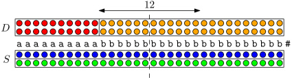
Figure 1: The coin flips for the input $\texttt{a}^{10}\texttt{b}^{22}\texttt{\#}$

In addition, the PFA keeps track of the difference $i-j$ modulo $12$. If $i\not\equiv j\pmod{12}$, the PFA declares the outcome to be “Different”.

If $i\equiv j\pmod{12}$, the outcome of the game is defined as follows. We call a coin lucky if it always came up heads.

• If $D$ has a lucky coin and $S$ has no lucky coin, declare “Different”.

• If $S$ has a lucky coin and $D$ has no lucky coin, declare “Same”.

• Otherwise, declare “Undecided”.

Since $i$ and $j$ are usually large, lucky actually means extremely lucky. Thus, the first two events are very rare, and the outcome will almost always be “Undecided”. The outcome of the Equality Checker is illustrated in Figure 2 and described in the following lemma.

Figure 2: The behavior of the Equality Checker, assuming $i\equiv j\pmod{12}$

• If $i=j$, $\Pr[\textup{``Different''}]=\Pr[\textup{``Same''}]$.

• If $i\neq j$, $\Pr[\textup{``Different''}]\geq 2^{11}\cdot\Pr[\textup{``Same''}]$.

Proof.

The first statement is clear, since each coin is flipped $2i$ times, and the situation between $D$ and $S$ is symmetric.

Assume that $i\neq j$. If $i\not\equiv j\pmod{12}$, then $\Pr[\textup{``Different''}]=1$, and we are done.

Otherwise, $|i-j|\geq 12$, and the smaller of $i$ and $j$, say $i$, is at most $i\leq\frac{i+j}{2}-6$. Then the red coin is flipped at most $2i\leq i+j-12$ times. Thus,

$$Pr[\text{$D$ has a lucky coin}]\geq Pr[\text{the red coin was lucky}]\geq 1/2^{i+j-12}$$ (3)

The blue and the green coin was each flipped $i+j$ times, and hence

$$Pr[\text{$S$ has a lucky coin}]\leq\\ Pr[\text{the blue coin was lucky}]+Pr[\text{the green coin was lucky}]\leq 2/2^{i+j}$$ (4)

The ratio ${Pr[\text{$D$ lucky}]}/{Pr[\text{$S$ lucky}]}$ between (3) and (4) is at least $2^{11}$. From each of these probabilities, we have to subtract the (small) probability that both $S$ and $D$ have a lucky coin, but this tilts the ratio between “Different” and “Same” even more in $D$’s favor. Formally:

$$\frac{\Pr[\textup{``Different''}]}{\Pr[\textup{``Same''}]}=\frac{\Pr[\text{$D$ lucky}]-\Pr[\text{$D$ lucky and $S$ lucky}]}{\Pr[\text{$S$ lucky}]-\Pr[\text{$D$ lucky and $S$ lucky}]}>\frac{\Pr[\text{$D$ lucky}]}{\Pr[\text{$S$ lucky}]}\geq 2^{11}\qed$$

Since the algorithm only needs to count up to 11 and to maintain a few flags, it is clear that it can be carried out by a PFA.

4.2 Correctness Test: checking a 2CM computation

Recall that we wish to check a description of a computation of the form

$$A=\texttt{0}^{l_{0}}\texttt{1}^{r_{0}}q_{0}\texttt{0}^{l_{1}}\texttt{1}^{r_{1}}{q_{1}}\texttt{0}^{l_{2}}\texttt{1}^{r_{2}}{q_{2}}\dots\texttt{0}^{l_{n}}\texttt{1}^{r_{n}}q_{n}\texttt{\#}\ .$$

The Equality Checker can be adapted to look at, say, two consecutive zero blocks $\texttt{0}^{l_{i}}$ and $\texttt{0}^{l_{i+1}}$ of a computation that represent the values of the counter $l$ and check whether $l_{i+1}={l_{i}}$. It can also be adapted to check $l_{i+1}=l_{i}+1$, or $l_{i+1}=l_{i}-1$, as appropriate for the state $q_{i}$ and the results of the zero test of $l_{i}$ and $r_{i}$. The guarantees of Lemma 4.1 about the outcome remain valid.

We run independent Equality Checkers for each relation between two consecutive values ${l_{i}}$ and ${l_{i+1}}$, as well as ${r_{i}}$ and ${r_{i+1}}$, of a computation $A$. In total, these are $2n$ Equality Checkers. In the schematic drawing of Figure 3, the outcomes of the Equality Checkers are shown as a row of boxes. Typically, most of them will be “Undecided”, with a few interspersed “Same” and “Different” results (proportionally much fewer than shown in the first example row). We are interested in the rare cases when all outcomes are “Same”, or all “Different”.

Figure 3: The Correctness Test for a computation $A$, and a hypothetical position where equality does not hold.

The output of these Equality Checkers is aggregated into a Correctness Test as follows: We report the output “CORRECT” if all Equality Checkers report “Same”, and we report the output “INCORRECT” if all Equality Checkers report “Different”. Otherwise, we report “NULL”.

To compute this result, only four independent Equality Checkers have to run simultaneously: While reading the input, the current block lengths $l_{i}$ and $r_{i}$ have to be compared with the preceding and the next values. Thus, the computation can be implemented by a PFA, with finitely many states. (Looking more carefully, one sees that actually, only three Equality Checkers are active at the same time: For example, when reading $\texttt{1}^{r_{i}}$, the Equality Check between $\texttt{0}^{l_{i-1}}$ and $\texttt{0}^{l_{i}}$ has already been completed.)

Suppose that a computation $A$ of the form (2) passes all formal checks.

If $A$ represents an accepting computation,

$$\Pr[\textup{``INCORRECT''}]=\Pr[\textup{``CORRECT''}].$$

If $A$ does not represent an accepting computation,

$$\Pr[\textup{``INCORRECT''}]\geq 2^{11}\cdot\Pr[\textup{``CORRECT''}].$$

Proof.

The probability for “CORRECT” is the product of the probabilities that each Equality Checker results in “Same”, and analogously, for “INCORRECT” and “Different”.

If $A$ represents an accepting computation, then all Equality Checkers are balanced between “Same” and “Different”, and the result is clear. Otherwise, there is at least one position (marked by an arrow in Figure 3) where an error occurs, and the probability for “Different” is at least $2^{11}$ times larger than for “Same”, according to Lemma 4.1. In all other Equality Checkers, the probability is either balanced or it gives a further advantage for “Different”. Thus, the product of the probabilities is at least $2^{11}$ times larger for “all Different” than for “all Same”. ∎

4.3 Third-level aggregation: processing the whole input

An Equality Checker aggregates the results of many coin flips into an output “Same”, “Different”, or “Undecided”. We have further aggregated the result of many Equality Checkers into a Correctness Test for the word $A$ (with output “CORRECT”, “INCORRECT”, or “NULL”). We add yet another level of aggregation in order to decide whether the PFA should accept the input word. As mentioned, we feed the PFA with a huge number of copies of an accepting computation $A$. Each copy of $A$ is subjected to the Correctness Test.

If we take the first definite result (“CORRECT” or “INCORRECT”) as an indication whether to accept or reject the input, we get an acceptance probability close to $1/2$ on a valid input. (It is a little less than $1/2$ because of the chance that the input runs out before a definite answer is obtained.) On the other hand, if there is no accepting computation, any input must consist of “fake” computations. The algorithm will recognize this and reject with probability at least $1-1/2^{11}$.

4.3.1 Increasing the acceptance probability

We modify the rules to make the acceptance probability larger, at the expense of the rejection probability for fake inputs. We determine the overall result as follows. As soon as a Correctness Test yields “CORRECT”, we accept the input. However, in order to reject the input, we wait until we have received 10 answers “INCORRECT” before receiving an answer “CORRECT”. If the end of the input is reached before any of these events happens, this also leads to rejection. Of course, we also reject the input right away if any of the formal checks fails.

If there is an accepting computation $A$ for the 2-CM, then the PFA accepts the input $A^{t}$, for sufficiently large $t$, with probability more than $0.99$.

If there is no accepting computation, then the PFA rejects every input with probability at least $0.99$.

Proof.

If $A$ is an accepting computation, the distribution between “CORRECT” and “INCORRECT” is fair. Thus, the probability of receiving 10 outputs “INCORRECT” before receiving an output “CORRECT” is $1/2^{10}<0.001$. To this we must add the probability of rejection because the input runs out before receiving an output “CORRECT”, but this can be made arbitrarily small by increasing $t$.

If there is no accepting computation, then “INCORRECT” has an advantage over “CORRECT” by a factor at least $2^{11}$. If the input runs out before a decision is reached, this is in the favor of rejection. Otherwise, the probability of receiving 10 outputs “INCORRECT” before receiving an output “CORRECT” is at least

$$\left(\frac{2^{11}}{2^{11}+1}\right)^{10}=\left(1-\frac{1}{2^{11}+1}\right)^{10}\geq(1-\tfrac{1}{2000})^{10}\approx 1-\tfrac{1}{200}=0.995.\qed$$

If the 2CM halts, there is an accepting computation $A$. ($A$ is unique since the 2CM is deterministic.) In this situation, the language recognized by the PFA with cut-point $\lambda=\frac{1}{2}$ contains the set $\{\,A^{t}\mid t\geq t_{0}\,\}$ for some large $t_{0}$. Otherwise, the language is empty.

As a consequence, checking whether the language accepted by a PFA is empty is undecidable.

4.3.2 Who is afraid of small probabilities?

As an exercise, we estimate the necessary number $t$ of repetitions of $A$. Suppose that the accepting computation $A$ has $m$ transitions. Then the counter values $l_{i}$ and $r_{i}$ are also bounded by $m$. The probability of the outcome “Same” in the Equality Checker is roughly $2^{-m}$, and the probability that all $2m$ Equality Checkers for the computation $A$ yield “Same”, leading to the answer “CORRECT”, is roughly $(2^{-m})^{2m}=4^{-m^{2}}$.

We want the probability that none of $t$ experiments gets the answer “CORRECT” to be $\leq 0.009$ (the difference between the bound $0.001>1/2^{10}$ established in the proof of Theorem 4.3.1 and the target tolerance $0.01$):

$$(1-4^{-m^{2}})^{t}\leq 0.009$$

Since $1-4^{-m^{2}}\approx\exp(-4^{-m^{2}})$, we need $t$ to be roughly $5\cdot 4^{m^{2}}$.

This dependence on the runtime $m$ of the 2-counter machine does not appear so terrible; however, when considering the overhead of simulating a Turing machine (see footnote 2), the dependence blows up to a triply-exponential growth in terms of the runtime of a Turing machine.

4.3.3 Boosting the decision probabilities

We can boost the decision probabilities beyond 0.99 to become arbitrarily close to 1. We simply run an odd number of copies of the PFA simultaneously and take a majority vote.

Alternatively, we can adjust the parameters. The number $K$ of times that we wait for “INCORRECT” before rejecting the input can be increased above $K=10$. As a compensation, we have to increase the modulus $G$ (we have chosen $G=12$) by which $i$ and $j$ are compared in the Equality Checker. The acceptance probability in case of a valid input increases to become arbitrarily close to $1-1/2^{K}$, and the rejection probability for an invalid input is at least $(1-1/2^{G-1})^{K}$.

In summary, for any $\varepsilon>0$ we can construct the PFA in such a way that it either accepts some word with probability at least $1-\varepsilon$, or there is no word that it accepts with probability larger than $\varepsilon$. This does not mean that there cannot be words whose acceptance probability is between those ranges, for example close to $1/2$. Candidates for such words are the words $A^{t}$ where $t$ is slightly too small.

4.4 Summing up the proof of Theorem 2

We have described the algorithm for the PFA verbally as a probabilistic algorithm, keeping in mind the finiteness constraints of a finite automaton. Eventually, this algorithm must be translated into a set of states and transition matrices. Theorem 2 puts some extra constraints on the PFAs whose emptiness is undecidable.

See 2

Proof.

The extra constraints can be easily fulfilled:

(a) We encode the input $A$ with a fixed-length binary code for the original input alphabet $Q\cup\{\texttt{0},\texttt{1},\texttt{\#}\}$. This means that the set $\mathcal{M}$ can be restricted to only two matrices. (Lemma 7.6 in Section 7.6 below treats this transformation more formally.)

(b) By padding the input, we can ensure that the PFA algorithm needs to toss at most one coin per input symbol, and thus the entries of the matrices can be restricted to $0,\frac{1}{2},1$. In the algorithm as described, only 16 coin tosses are necessary per input character (four coins per Equality Checker running at any point in time). Thus we simply pad each codeword in the binary code with 15 zeros.

(c) Our algorithm does not need to make any coin flips before reading the first symbol. Thus, we can fix the starting state to be a deterministic state.

(d) Finally, a single accepting state is enough: As soon as the algorithm has decided to accept the input, it will stay committed to this decision. The accepting state is an absorbing state, and there is another absorbing state for rejection. In terms of vectors, both the starting distribution $\pi$ and the characteristic vector $f$ of accepting states are standard unit vectors. (Since the empty input is not accepted, the accepting state is distinct from the starting state, and we can arrange the states so that the acceptance probability is found in the upper right corner of the product $M_{1}M_{2}\ldots M_{m}$.) ∎

4.5 History of ideas

Condon and Lipton credit the main ideas of their proof to Rūsiņš Freivalds [8], who studied the emptiness problem for probabilistic 2-way finite automata in 1981 (unaware of Nasu and Honda’s earlier work). In particular, Freivalds developed the idea of a competition between two players to recognize the language $\{\,\texttt{a}^{i}\texttt{b}^{i}\mid i\geq 0\,\}$ (Section 4.1), and aggregating the results of these competitions into “macrocompetitions” (Section 4.2). A 2-way automaton can move the input head back and forth over the input, and thus process the input as often as it wants. Freivalds claimed that the emptiness problem for such automata is undecidable [8, Theorem 4]; he gives only a hint that the reduction should be from the PCP (Post’s Correspondence Problem, see Section 5.2), without any details how to connect “macrocompetitions” with the PCP. I have not been able to come up with an idea how the proof would proceed.

For our present case of a (1-way) finite automaton, the repeated scan of the input is not possible; it is replaced by providing an input which consists of many repetitions of the same word.

5 The Nasu–Honda–Claus proof via Post’s Correspondence Problem

This section presents the proof of Nasu and Honda [13] from 1969 in the version of Claus [4] from 1971, leading to the undecidability results in Propositions 1–4, which are then strengthened to Theorems 1–2 in the rest of the paper.

5.1 The binary PFA

For a string $u\in\{\texttt{0},\texttt{1}\}^{*}$, we denote by $(u)_{2}$ the numeric value of $u$ when it is interpreted as a binary number, and we write $|u|$ for the length of $u$. We define the stochastic matrix

$$B(u):=\begin{pmatrix}1-\frac{(u)_{2}}{2^{|u|}}&\frac{(u)_{2}}{2^{|u|}}\\[5.0pt] 1-\frac{(u)_{2}+1}{2^{|u|}}&\frac{(u)_{2}+1}{2^{|u|}}\end{pmatrix}\text{, for example }B(\texttt{00110})=\begin{pmatrix}\frac{26}{32}&\frac{6}{32}\\[5.0pt] \frac{25}{32}&\frac{7}{32}\end{pmatrix}.$$

Note that the top right entry $\frac{(u)_{2}}{2^{|u|}}$ of this matrix is the value $0.u$ when interpreted as a binary fraction; for example, $\frac{6}{32}=(0.00110)_{2}$. We will continue to use the convenient notation $0.u$ for this. These matrices fulfill the remarkable multiplication law

$$B(u)B(u^{\prime})=B(u^{\prime}u),$$ (5)

which can be confirmed by a straightforward calculation. Note the reversed order of the factors.

5.2 Post’s Correspondence Problem (PCP)

In the Post Correspondence Problem (PCP), we are given a list of pairs of strings $(v_{1},w_{1}),(v_{2},w_{2}),\ldots,(v_{k},w_{k})$. The problem is to decide if there is a nonempty sequence $a_{1}a_{2}\ldots a_{m}$ of indices $a_{i}\in\{1,2,\ldots,k\}$ such that

$$v_{a_{1}}v_{a_{2}}\ldots v_{a_{m}}=w_{a_{1}}w_{a_{2}}\ldots w_{a_{m}}$$

This is one of the well-known undecidable problems. It is no restriction to fix the alphabet to $\{\texttt{0},\texttt{1}\}$, since every alphabet can be encoded in binary.

Figure 4: The binary automaton with acceptance probability $\phi$

Let us look at the first sequence of strings $v_{1},\ldots,v_{k}$. We construct a PFA with input alphabet $\{1,2,\ldots,k\}$ and two states $\Phi_{0}$ and $\Phi_{1}$, see Figure 4. The transition matrices are $M_{i}=B(v_{i})$. We take $\Phi_{0}$ as the starting state and $\Phi_{1}$ as the accepting state. Then the acceptance probability of the word $a=a_{1}a_{2}\ldots a_{m}$ is found in the upper right corner of the product $M_{a_{1}}M_{a_{2}}\ldots M_{a_{m-1}}M_{a_{m}}$ of the corresponding transition matrices, and it follows from (5) that this is

$$\phi(a)=0.v_{a_{m}}v_{a_{m-1}}\ldots v_{a_{2}}v_{a_{1}}.$$ (6)

We can build an analogous PFA for the other sequence of strings $w_{1},\ldots,w_{k}$, and then the acceptance probability of $a$ will be

$$\psi(a)=0.w_{a_{m}}w_{a_{m-1}}\ldots w_{a_{2}}w_{a_{1}}.$$ (7)

Due to the swapping of the factors in the multiplication law (5), the strings are concatenated in (6) and (7) in reverse order, but this cosmetic change does not affect the undecidability of the PCP. Thus the PCP comes down to the question whether there is a nonempty word $a$ with equal acceptance probabilities $\phi(a)=\psi(a)$ in the two PFAs.

We have to be careful because of the trailing zeros issue: Trailing zeros don’t change the probabilities (6) and (7). An easy way to circumvent this problem is to add a 1 after every symbol of every string, thus doubling the length of the strings. This ensures that there are no trailing zeros that could go unnoticed.

5.3 Testing equality of probabilities

For recognizing the words $a$ with $\phi(a)=\psi(a)$, there is a construction of a PFA that does this job. It is based on the identity

$$\tfrac{1}{2}\phi\psi+\tfrac{1}{4}(1-\phi^{2})+\tfrac{1}{4}(1-\psi^{2})=\tfrac{1}{2}-\tfrac{1}{4}(\phi-\psi)^{2}.$$ (8)

We will build a PFA for each term $\phi\psi$, $1-\phi^{2}$, $1-\psi^{2}$ on the left, and we will mix them in the right proportion. As the right-hand side shows, we have then (almost) achieved our goal: The acceptance probability achieves its maximum value $\frac{1}{2}$ only for $\phi(a)=\psi(a)$.

Figure 5: Acceptance probability $\phi\psi$

It is straightforward to build a PFA whose acceptance probability is the product $\phi(a)\psi(a)$, see Figure 5: This PFA simulates the two PFAs for $v_{1},\ldots,v_{k}$ and for $w_{1},\ldots,w_{k}$ simultaneously and accepts if both PFAs accept. The resulting product PFA has four states $\{\Phi_{0},\Phi_{1}\}\times\{\Psi_{0},\Psi_{1}\}$. Similarly, we can build a PFA with acceptance probability $\phi(a)^{2}$: We simulate two independent copies of the PFA for $v_{1},\ldots,v_{k}$. This leads again to four states. To get acceptance probability $1-\phi(a)^{2}$, we complement the set of accepting states. The PFA for $1-\psi(a)^{2}$ follows the same principle. Finally, we mix the three PFAs in the ratio $\frac{1}{2}:\frac{1}{4}:\frac{1}{4}$, as shown in Figure 6a.

Figure 6: (a) Acceptance probability $\tfrac{1}{2}-\tfrac{1}{4}(\phi-\psi)^{2}$. (b) $\tfrac{1}{4}-\tfrac{1}{8}(\phi-\psi)^{2}+\varepsilon$

The dash-dotted arrows from the start state to three “local start states” inside the square boxes denote random transitions that should be thought of as happening before the algorithm reads its first input symbol. In the PFA, such a transition is actually carried out in combination with the subsequent transition for the input symbol inside one of the square boxes, as part of the transition out of the start state when reading the first input symbol.

The introduction of the new start state has the beneficial side effect of eliminating the empty word $\epsilon$ from the recognized language. The empty word would otherwise satisfy the equation $\phi(a)=\psi(a)$, because $\phi(\epsilon)=\psi(\epsilon)=0$.

In total, we have now 13 states, 7 of which are accepting. As an intermediate undecidability result, we can thus state:

Proposition 1.

The following problem is undecidable:

Given a finite set $\mathcal{M}$ of stochastic matrices of size $13\times 13$ with binary fractions as entries, is there a product $M_{1}M_{2}\ldots M_{m}$, with $M_{i}\in\mathcal{M}$ for all $i=1,\ldots,m$, such that the sum of the $7$ rightmost entries in the top row is $\geq\tfrac{1}{2}$? ∎

5.4 Achieving strict inequality

Proposition 1 almost describes a PFA, except that the convention for a PFA to recognize a word is strict inequality ($>\lambda$). We thus have to raise the probability just a tiny bit, without raising any of the values $<\lambda$ to become bigger than $\lambda$.

Since all probabilities are rational, this can be done as follows, see Figure 6b. In our case, all transition probabilities within the square boxes are multiples of some small unit

$$\gamma:=4^{-\max\{|v_{i}|,|w_{i}|:1\leq i\leq k\}}.$$

The original PFA is entered with probability 1/2. The transition probabilities from the start state into the original PFA are now multiples of $\gamma/8$. (Remember that such a transition consists of a transition from the start state along a dash-dotted arrow combined with a transition inside a square box.) We create a new accepting state $q_{A}$ that is chosen initially with probability $1/{16}$. Whenever a symbol is read, the PFA stays in that state with probability $\gamma$, and otherwise it moves to some absorbing state $q_{R}$. With the remaining probability $7/{16}$, we go to $q_{R}$ directly.

The new part contributes $\varepsilon:=\frac{1}{16}\gamma^{|a|}$ to the acceptance probability of every nonempty word $a$. From the old part we have $\tfrac{1}{4}-\tfrac{1}{8}(\phi-\psi)^{2}$, and we know that this probability is a multiple of $\frac{1}{8}\gamma^{|a|}=2\varepsilon$. Thus, if this probability is less than $1/4$, it cannot become greater than $1/4$ by adding $\varepsilon$. If it was equal to $1/4$ (i.e., if $a$ is a solution to the PCP), it becomes greater than $1/4$.

Proposition 2.

It is undecidable whether the language recognized by a PFA with 15 states with cut-point $\lambda=1/4$ is empty. ∎

This PFA has a fixed starting state.

The cut-point can be changed to any positive rational value less than 1/2 by adjusting the initial split probability between the original PFA of Figure 6a and the states $q_{A}$ and $q_{R}$. Cut-points between 1/2 and 1 can be achieved at the expense of adding another accepting state.

According to Neary [14], the PCP is already undecidable with as few as five string pairs. Therefore, the size of the input alphabet in Proposition 2, or the number of matrices $\mathcal{M}$ in Proposition 1 can be restricted to 5.

5.5 History of ideas

The binary automaton (Section 5.1) and its generalization to other radices than 2 appears already in Rabin’s 1963 paper [19], and it is credited to E. F. Moore. The basic $m$-ary automaton processes single digits from $\{0,\ldots,m-1\}$. The binary automaton matrix in Section 5.1 for variable-length input words $u$ is the product of several such single-digit matrices. Instead of binary automata, Nasu and Honda [13] use ternary (triadic) automata with digits $\{\mathtt{0},\texttt{1},\texttt{2}\}$, of which only $\{\texttt{1},\texttt{2}\}$ are used in order to avoid the trailing zeros issue.

The equality test for probabilities (constructing a PFA to accept words $a$ with $\phi(a)=\psi(a)$ from two PFAs with acceptance probabilities $\phi(a)$ and $\psi(a)$, Section 5.3), including the method of adding a small probability to change $\geq\lambda$ into $>\lambda$ (Section 5.4) is given in Nasu and Honda [13, Lemma 11, pp. 259–260]. The authors credit H. Matuura, Y. Inagaki, and T. Hukumura for the key ideas (a technical report and a conference record, both from 1968 and in Japanese) [13, p. 261].

Claus already observed [4, p. 158, remark after the proof of Satz 28] that the construction leads to a bounded number of states. The details have been worked out above.

As I haven’t been able to survey the rich literature on probabilistic automata, I may very well have overlooked some earlier roots of these ideas.

Nasu and Honda [13], in a footnote to Theorem 21, their main result about the undecidability of PFA Emptiness, write that “it reduces to a statement in p. 150” of a paper of Marcel Schützenberger [23] from 1963 [13, footnote 6 on p. 270, referring to the remark before Lemma 12, p. 261]. In that paper, Schützenberger derives some undecidability results, using, among others, the PCP, but I am not able to see the connection.

Nasu and Honda prove the undecidability of two more questions in connection with the language recognized by a PFA: whether the language is regular, or whether the language is context-free [13, Theorem 22, p. 270], see Appendix A.1.

5.6 Saving two states by merging indistinguishable states

In the PFA with acceptance probability $\phi(a)^{2}$, where we simulate two independent copies of the same PFA, we can see that the states $(\Phi_{0},\Psi_{1})$ and $(\Phi_{1},\Psi_{0})$ of Figure 5 become indistinguishable when $\phi=\psi$. Thus, they can be merged into one state, denoted by $\{\Phi_{0},\Phi_{1}\}$, and we reduce the number of states by one, see Figure 7a–b.

​​​​

Figure 7: (a) Acceptance probability $1-\phi^{2}$ with 4 states (b) with 3 states. (c) Acceptance probability $\tfrac{1}{4}-\tfrac{1}{8}(\phi-\psi)^{2}+\varepsilon$ with 13 states

More precisely, if we denote the transition probabilities of the original binary automaton by

$$B(u)=\raise 6.45831pt\hbox{$\begin{array}[]{c@{\quad}cc}&\Phi_{0}&\Phi_{1}\\[1.0pt] \Phi_{0}&\smash{\lower 7.3194pt\hbox to0.0pt{\hss$\left(\vbox to12.91663pt{}\right.$}}p_{00}&p_{01}\smash{\lower 7.3194pt\hbox to0.0pt{$\left.\vbox to12.91663pt{}\right),$\hss}}\\ \Phi_{1}&p_{10}&p_{11}\end{array}$}$$

the 3-state PFA has the following transition matrix:

$$\begin{array}[]{c@{\ \quad}ccc}&(\Phi_{0},\Phi_{0})&\{\Phi_{0},\Phi_{1}\}&(\Phi_{1},\Phi_{1})\\[3.0pt] (\Phi_{0},\Phi_{0})&p_{00}^{2}&2p_{00}p_{01}&p_{01}^{2}\\ \{\Phi_{0},\Phi_{1}\}&\hbox to0.0pt{\hss\smash{$\left(\vbox to19.37494pt{}\right.$}}p_{00}p_{10}&p_{01}p_{10}+p_{00}p_{11}&p_{01}p_{11}\hbox to0.0pt{\smash{$\left.\vbox to19.37494pt{}\right)$}\hss}\\ (\Phi_{1},\Phi_{1})&p_{10}^{2}&2p_{10}p_{11}&p_{11}^{2}\end{array}$$ (9)

When the reduced automaton is in the state $\{\Phi_{0},\Phi_{1}\}$, we can think of the original 4-state automaton being in one of the states $(\Phi_{0},\Phi_{1})$ or $(\Phi_{1},\Phi_{0})$, each with probability $1/2$.

For the PFAs in Propositions 1 and 2, the number of states can thus be reduced by 2, as stated in the following proposition. Figure 7c illustrates the automaton for Proposition 3b. We will show some explicit examples of transition matrices for this automaton below, in Section 6.5.

Proposition 3.

1. The following problem is undecidable:

   Given a finite set $\mathcal{M}$ of stochastic matrices of size $11\times 11$ with binary fractions as entries, is there a product $M_{1}M_{2}\ldots M_{m}$, with $M_{i}\in\mathcal{M}$ for all $i=1,\ldots,m$, such that the sum of the 5 rightmost entries in the top row is $\geq\tfrac{1}{2}$?

2. It is undecidable whether the language recognized by a PFA with 13 states with cut-point $\lambda=1/4$ is empty. ∎

5.7 Saving the starting state by using the Modified Post Correspondence Problem

We can eliminate the starting state by using the Modified Post Correspondence Problem (MPCP). It differs from the PCP in one detail: The pair $(v_{1},w_{1})$ must be used as the starting pair, and it cannot be used in any other place. In other words, the solution must satisfy the constraints $a_{1}=1$, and $a_{i}>1$ for $i=2,\ldots,m$. The MPCP is often used as an intermediate problem when reducing the Halting Problem for Turing machines to the PCP, and then it takes some extra effort to reduce the MPCP to the PCP, see for example [9, Lemma 8.5] or [24, p. 189]. In our situation, the MPCP is actually the more convenient version of the problem.

The idea is to apply the transition for the first letter $a_{1}$ right away, and use the resulting distribution on the states as the starting distribution $\pi$.

There is still a small technical discrepancy: In the formulas (6) and (7) for the acceptance probability, the first letter of the sequence $a$ determines the last pair of strings to be concatenated. Thus we must reverse all strings $v_{i}$ and $w_{i}$ and turn the MPCP into a reversed MPCP, where the last pair in the concatenation is prescribed to be the pair $(v_{1},w_{1})$:

The Reversed Modified Post Correspondence Problem (RMPCP).

We are given a list of pairs of strings $(v_{1},w_{1}),(v_{2},w_{2}),\ldots(v_{k},w_{k})$ over the alphabet $\{\texttt{0},\texttt{1}\}$ such that $v_{1}$ and $w_{1}$ end with 1. The problem is to decide if there is a sequence $a_{2},\ldots,a_{m}$ of indices $a_{i}\in\{2,\ldots,k\}$ such that

$$v_{a_{m}}v_{a_{m-1}}\ldots v_{a_{2}}v_{1}=w_{a_{m}}w_{a_{m-1}}\ldots w_{a_{2}}w_{1}\ .$$

This is of course just a trivial variation of the MPCP. The translation of (6) and (7) can now be applied directly. Moreover, the trailing zeros issue disappears, since $v_{1}$ and $w_{1}$ end with 1. This extra condition can be easily fulfilled by appending a 1 to $v_{1}$ and $w_{1}$ if necessary.

Proposition 4.

It is undecidable whether the language recognized by a PFA with 12 states with cut-point $\lambda=1/4$ is empty.

Proof.

The above construction that has led to Proposition 3b gives a set of $13\times 13$ matrices such that the index sequence $a_{1}a_{2}\ldots a_{m}$ is a solution of the PCP if and only if

$$e_{1}^{T}M_{a_{1}}M_{a_{2}}\ldots M_{a_{m-1}}M_{a_{m}}f>\tfrac{1}{4},$$

where $e_{1}$ is the first unit vector $(1,0,\ldots,0)$ and $f$ is a vector with 6 zeros and 7 ones. For every other index sequence, the value of the expression is $<\frac{1}{4}$.

For the reversed MPCP the first matrix $M_{a_{1}}=M_{1}$ is specified. Thus the product $e_{1}^{T}\!M_{1}$ has a fixed value $\pi^{T}$, and we can replace it by this vector:

$$\pi^{T}\!M_{a_{2}}\ldots M_{a_{m-1}}M_{a_{m}}f$$

This is the expression for the acceptance probability starting from an initial probability distribution $\pi$. The remaining matrix product is not allowed to use $M_{1}$, and this is easily ensured by removing $M_{1}$ from $\mathcal{M}$.

The original PFA goes from the start state to the 12 other states and never returns to the start state; thus we can eliminate the start state and only use the $12\times 12$ submatrices for the remaining states. ∎

We mention that with cut-point $\frac{1}{2}$ and the weak inequality $\geq\tfrac{1}{2}$ as acceptance criterion instead of $>\tfrac{1}{4}$, we don’t need the extra states $q_{A}$ and $q_{R}$, and the number of states is reduced to 10.

6 Fixing the set of matrices by using a universal Turing machine

We can achieve stronger and more specific results by tracing back the undecidability of the PCP to the Halting Problem. In particular, we will look at a universal Turing machine and derive from it a “universal” PCP. A universal Turing machine is a fixed Turing Machine that can simulate any other Turing machine. In particular, the Halting Problem for such a machine is undecidable: Given some initial contents of the tape, does the machine halt? Sticking to one fixed machine allows us to choose a fixed set of matrices that represents the PFA. The only variation is the starting distribution $\pi$, or, in another variation, the vector $f$ of output values.

6.1 Constructing an MPCP for a Turing machine

In order to adhere to the usual practice, we describe the translation to the MPCP and not to the reversed MPCP. (For applying the RMPCP, the strings simply have to be reversed.) Also, we temporarily use a general alphabet for the string pairs of the MPCP. In the end, this alphabet will be encoded into the binary alphabet $\{\texttt{0},\texttt{1}\}$ in order to be translated into a PFA.

The word $v_{a_{1}}v_{a_{2}}\ldots v_{a_{m}}=w_{a_{1}}w_{a_{2}}\ldots w_{a_{m}}$ is built as a concatenation of successive configurations of the Turing machine, separated by the marker #. The words are built incrementally in such a way that the partial word $v_{1}v_{a_{2}}\ldots v_{a_{n}}$ lags one step (of the Turing machine) behind the partial word $w_{1}w_{a_{2}}\ldots w_{a_{n}}$. Figure 8 shows an example.

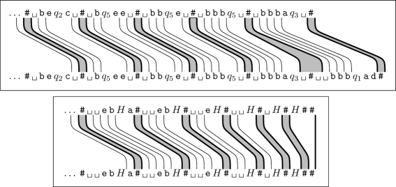
Figure 8: Top: Building two partial words $v_{1}v_{a_{2}}\ldots v_{a_{n}}$ (upper row in each box) and $w_{1}w_{a_{2}}\ldots w_{a_{n}}$ (lower row) for a Turing machine with transition rules $(q_{2},\texttt{c},\texttt{e},L,q_{5})$, $(q_{5},\texttt{e},\texttt{b},R,q_{5})$, $(q_{5},\texttt{\char 32\relax},\texttt{a},R,q_{3})$, $(q_{3},\texttt{\char 32\relax},\texttt{d},L,q_{1})$, among others. For better visibility, the correspondences involving the separator # are highlighted. Near the right end, the padding pair $(\texttt{\#},\texttt{{\char 32\relax}\#{\char 32\relax}})$ is used once in order to produce extra blanks at the ends of the tape, preventing the state symbol $q_{3}$ from becoming adjacent to the marker #. Bottom: After the Turing machine has halted, the tape is cleared and the common word is completed.

Following the common convention, a string such as #␣be$q_{2}$c␣# denotes the configuration where the Turing machine is in state $q_{2}$, the tape contains the symbols bec padded by infinitely many blank symbols on both sides (of which two are present in the string), and the Turing machine is positioned over the third occupied cell, the one with the symbol c.

The transition rules of the Turing machine are translated into pairs $(v_{i},w_{i})$, as will be described below. The important feature of this translation is shown in Figure 9: The input for the Turing machine is translated into the starting pair $(v_{1},w_{1})$. In the above translation to a PFA, leading to Proposition 4, the starting pair $(v_{1},w_{1})$ affects only the starting distribution $\pi$, whereas the transition matrices $M_{i}$ depend only on the rules of the Turing machine, which, for a universal Turing machine, are fixed!

Figure 9: How the PFA is constructed from a Turing machine via an MPCP

6.2 List of string pairs of the MPCP

Since we want a MPCP with as few pairs as possible, we review the construction of the MPCP from the Turing machine in detail. We follow the construction from Sipser [24, Section 5.2, Part 5, p. 187] to ensure that the configurations are padded with sufficiently many blank symbols. This eliminates the need to deal with special cases when the Turing machine reaches the “boundary” of the tape in the representation as a finite string.

Let $\Gamma$ denote the tape alphabet including the blank symbol ␣, and let $Q$ denote the set of states of the Turing machine. The strings $v_{i}$ and $w_{i}$ of the MPCP use the alphabet $\Gamma\cup Q\cup\{\texttt{\#},H\}$ with two extra symbols: a separation symbol # and a halting symbol $H$.

• If the input word for the Turing machine is $u\in\{\texttt{0},\texttt{1}\}^{*}$, we define the starting pair $(v_{1},w_{1})=(\texttt{\#},\texttt{\#{\char 32\relax}}q_{0}u\texttt{{\char 32\relax}\#})$, where $q_{0}$ is the start state of the Turing machine.

The other pairs $(v_{i},w_{i})$ are as follows:

• For copying from the shorter word to the more advanced word, we have the pairs $(s,s)$ for all $s\in\Gamma$.

• We have another copying pair $(\texttt{\#},\texttt{\#})$, and the padding pair $(\texttt{\#},\texttt{{\char 32\relax}\#{\char 32\relax}})$. We are allowed to (nondeterministically) emit an additional blank symbol at both ends of the configuration.

• For each right-moving rule $(q,s,s^{\prime},R,q^{\prime})$, the pair $(qs,s^{\prime}q^{\prime})$. (Such a rule means that when the Turing machine is in state $q$ and reads the tape symbol $s$, it overwrites the symbol $s$ with $s^{\prime}$, moves one step to the right on the tape, and changes to state $q^{\prime}$.)

• For each left-moving rule $(q,s,s^{\prime},L,q^{\prime})$ and for each $t\in\Gamma$, the pair $(tqs,q^{\prime}ts^{\prime})$.

• For each halting rule $(q,s,-)$, the pair $(qs,H)$. The character $H$ represents the fact that the machine has halted.

• For each $s\in\Gamma$, the erasing pairs $(Hs,H)$ and $(sH,H)$. The halting symbol absorbs all symbols on the tape one by one.

• Finally, the finishing pair $(H\texttt{\#\#},\texttt{\#})$. This is the only way how the two words can come to a common end.

In total, these are $3|\Gamma|+3$ pairs, plus $|\Gamma|$ pairs for each left-moving rule, plus one pair for each right-moving or halting rule, plus the starting pair.

6.3 Using a universal Turing machine

We have looked at the parameters of various universal Turing machines in the literature in order to see which ones give the smallest number of pairs $(v_{i},w_{i})$ for our PCP. The best result is obtained from the machine $U_{15,2}$ of Neary and Woods [15, Section 3.5]. Its tape alphabet, including the blank symbol, has size $|\Gamma|=2$. It has 15 states, not counting the halting state. It has 15 left-moving rules, 14 right-moving rules, and 1 halting rule. In terms of PCP pairs, left-moving rules are more costly than right-moving rules, but we have the freedom to swap left-moving with right-moving rules by flipping the Turing machine’s tape. We have to switch to the nonstandard convention of starting the Turing machine over the rightmost input character, but this is easily accomplished in the construction of the starting pair $(v_{1},w_{1})$. Thus, with 14 left-moving rules and 16 right-moving and halting rules, we get $3\times 2+3+14\times 2+16=53$ pairs, plus the starting pair $(v_{1},w_{1})$ that encodes the input.

In some sense, this can be regarded as a universal MPCP: all pairs except the starting pair are fixed.

We can now establish a weaker version of Theorem 1b, with matrices of dimension $12\times 12$ instead of $11\times 11$.

Proposition 5.

There is a fixed set of 53 stochastic matrices $\mathcal{M}^{\prime\prime\prime\prime}$ of dimension $12\times 12$, whose entries are multiples of $2^{-22}$, and a fixed $0$-$1$-vector $f\in\{0,1\}^{12}$, for which the following question is undecidable:

Given a probability distribution $\pi\in\mathbb{Q}^{12}$ whose entries are binary fractions, is there a product $M_{1}M_{2}\ldots M_{m}$, with $M_{i}\in\mathcal{M}^{\prime\prime\prime\prime}$ for all $i=1,\ldots,m$, such that

$$\pi^{T}\!M_{1}M_{2}\ldots M_{m}f>\tfrac{1}{4}\ ?$$

In other words, is the language recognized by the PFA with starting distribution $\pi$ and cut-point $\lambda=\frac{1}{4}$ nonempty?

Proof.

We specialize the proof of Proposition 4 to the current setting. The important point, as discussed above and shown in Figure 9, is that the matrices in $\mathcal{M}$ depend only on the string pairs that reflect the rules of the universal Turing machine $U_{15,2}$, which are fixed, and we have already calculated that there are 53 of these matrices.

We must not forget that the symbols of the alphabet $\Gamma\cup Q\cup\{\texttt{\#},H\}$, in which the string pairs $(v_{i},w_{i})$ of the MPCP are written, have to be encoded somehow into the binary alphabet $\{\texttt{0},\texttt{1}\}$ in order to define the matrices of the PFA, and we have to ensure that the codes of $v_{1}$ and $w_{1}$ end with 1, for example by letting the code for # end with 1.

There is one technicality that needs to be resolved. The quantity $\gamma$ was required to be a common divisor of the matrix entries, and it depends on the maximum lengths $|v_{i}|$ and $|w_{i}|$ of the input strings. However, the strings $v_{1}$ and $w_{1}$ depend on the input tape, and thus, their lengths $|v_{1}|$ and $|w_{1}|$ cannot be bounded in advance. (The remaining strings depend only on the Turing machine.) The solution is to carry out the imagined first transition (which is not encoded into a transition matrix in $\mathcal{M}$, but determines the starting distribution $\pi$) with a sufficiently small value of $\gamma$, namely $\gamma_{1}=4^{-\max\{|v_{1}|,|w_{1}|\}}$, where the lengths $|v_{1}|$ and $|w_{1}|$ are measured in the binary encoding. The other transitions from the state $q_{A}$ can be carried out with the fixed value $\gamma$ that is sufficient for those entries. Table 2 shows the starting distribution $\pi$ resulting from this construction. Since $\pi$ is allowed to depend on the input, we have solved the problem.

state $q$	$\pi_{q}$	state $q$	$\pi_{q}$	state $q$	$\pi_{q}$
$(\Phi_{0},\Psi_{0})$	$\!\frac{1}{4}(1-0.v_{1})(1-0.w_{1})\!$	$(\Phi_{0},\Phi_{0})$	$\frac{1}{8}(1-0.v_{1})^{2}$	$\{\Psi_{0},\Psi_{1}\}$	$\!\frac{1}{4}(1-0.w_{1})0.w_{1}\!$
$(\Phi_{0},\Psi_{1})$	$\frac{1}{4}(1-0.v_{1})0.w_{1}$	$\{\Phi_{0},\Phi_{1}\}$	$\frac{1}{4}(1-0.v_{1})0.v_{1}$	$(\Psi_{1},\Psi_{1})$	$\frac{1}{8}(0.w_{1})^{2}$
$(\Phi_{1},\Psi_{0})$	$\frac{1}{4}\cdot 0.v_{1}(1-0.w_{1})$	$(\Phi_{1},\Phi_{1})$	$\frac{1}{8}(0.v_{1})^{2}$	$q_{A}$	$\frac{1}{16}\gamma_{1}$
$(\Phi_{1},\Psi_{1})$	$\frac{1}{4}\cdot 0.v_{1}\cdot 0.w_{1}$	$(\Psi_{0},\Psi_{0})$	$\frac{1}{8}(1-0.w_{1})^{2}$	$q_{R}$	$\frac{1}{2}-\frac{1}{16}\gamma_{1}$

Table 2: Starting probabilities $\pi$ for Proposition 5

We have now established the existence of 53 fixed matrices $\mathcal{M}^{\prime\prime\prime\prime}$ and a finishing 0-1-vector $f$ for which the decision problem of Proposition 5 is undecidable.

6.4 An efficient code

In order to say something about the entries of these matrices, we have to be more specific about the way how the alphabet $\Gamma\cup Q\cup\{\texttt{\#},H\}$ is encoded. The strings $v_{i}$ and $w_{i}$ that come from the Turing machine rules are actually quite short: they have at most 3 letters. More precisely, they consist of at most one “state” symbol from $Q\cup\{H\}$, plus at most two letters from the tape alphabet $\Gamma\cup\{\texttt{\#}\}$. The Turing machine $U_{15,2}$ has $|Q|=15$ states and a tape alphabet of size $|\Gamma|=2$.

In this situation, a variable-length code is more efficient than a fixed-length code. We can use 5-letter codes of the form 0**** for the 15 states plus the halting state $H$. This leaves the 3-letter codes 1** for the 3 symbols $\Gamma\cup\{\texttt{\#}\}$, leading to string lengths bounded by $5+3+3=11$. In the binary automaton, the transition probabilities are therefore multiples of $2^{-11}$. Since each box carries out two binary automata simultaneously, the transition probabilities are multiples of $4^{-11}$. ∎ With a weak inequality like $\geq\tfrac{1}{2}$ instead of $>\tfrac{1}{4}$ as acceptance criterion, we don’t need the extra states $q_{A}$ and $q_{R}$, and the size of the matrices for which Proposition 5 holds can be reduced to $10\times 10$.

As mentioned after Proposition 2, the cut-point can be changed to a different value; in that case, the constraint that the input distribution $\pi$ consists of binary fractions must be abandoned. Since the change only affects the very first transition, the fixed matrix set $\mathcal{M}$ remains unchanged.

The above variable-length code seems to be pretty efficient, but it wastes one of the four codewords 1**. By looking at the actual rules of the machine $U_{15,2}$ and fiddling with the code, it might be possible to improve the power $22$ in the denominator of the binary fractions.

6.5 Example matrices

For illustration, we compute some matrices of the set $\mathcal{M}^{\prime\prime\prime\prime}$ explicitly. We use the binary code $\texttt{\#}\doteq\texttt{101}$, $\texttt{{\char 32\relax}}\doteq\texttt{100}$. The copying pair $(\texttt{\char 32\relax},\texttt{\char 32\relax})\doteq(\mathtt{100},\mathtt{100})$ is then translated into the block diagonal matrix

$$\overline{M}_{(\texttt{\char 32\relax},\texttt{\char 32\relax})}=\begin{pmatrix}\small\dfrac{1}{64}\left(\begin{array}[]{@{\,}r@{\ }r@{\ }r@{\ }r@{\,}}16&16&16&16\\ 12&20&12&20\\ 12&12&20&20\\ 9&15&15&25\end{array}\right)&0&0&0&0\\ 0&\small\dfrac{1}{64}\small\left(\begin{array}[]{@{\,}r@{\ }r@{\ }r@{\,}}16&32&16\\ 12&32&20\\ 9&30&25\end{array}\right)&0&0&0\\ 0&0&\dfrac{1}{64}\small\left(\begin{array}[]{@{\,}r@{\ }r@{\ }r@{\,}}16&32&16\\ 12&32&20\\ 9&30&25\end{array}\right)&0&0\\ 0&0&0&\frac{1}{2^{22}}&1-\frac{1}{2^{22}}\\ 0&0&0&0&1\end{pmatrix},$$

where the rows and columns correspond to the states as they are ordered in Table 2. We use a bar in the notation $\overline{M}_{(\texttt{\char 32\relax},\texttt{\char 32\relax})}$ to remind us of the fact that we are dealing with the reversed MPCP, and therefore the strings should be reverse (which, in this case, has no effect because we have only one-letter strings).

Let us look at the erasing pair $(\texttt{\#{\char 32\relax}},\texttt{\#})$. Here the reversal does have an effect, and the strings are actually $(\texttt{{\char 32\relax}\#},\texttt{\#})\doteq(\mathtt{100\,101},\mathtt{101})$. (The codewords don’t have to be reversed.) With these data, the matrix $\overline{M}_{(\texttt{\#{\char 32\relax}},\texttt{\#})}$ looks as follows:

$$\begin{pmatrix}\small\dfrac{1}{512}\left(\begin{array}[]{@{\,}r@{\ }r@{\ }r@{\ }r@{\,}}81&135&111&185\\ 54&162&74&222\\ 78&130&114&190\\ 52&156&76&228\end{array}\right)&0&0&0&0\\ 0&\small\dfrac{1}{4096}\small\left(\begin{array}[]{@{\,}r@{\ }r@{\ }r@{\,}}729&1998&1369\\ 702&1988&1406\\ 676&1976&1444\end{array}\right)&0&0&0\\ 0&0&\dfrac{1}{64}\small\left(\begin{array}[]{@{\,}r@{\ }r@{\ }r@{\,}}9&30&25\\ 6&28&30\\ 4&24&36\end{array}\right)&0&0\\ 0&0&0&\frac{1}{2^{22}}&1-\frac{1}{2^{22}}\\ 0&0&0&0&1\end{pmatrix}$$

Finally, as our most elaborate example, we consider a left-moving rule of the Turing machine $U_{15,2}$ from [15]: $(q_{9},\texttt{\char 32\relax},\texttt{\char 32\relax},L,q_{1})$. This was originally a right-moving rule, but has been converted into a left-moving rule by flipping the tape. It produces two string pairs, since $|\Gamma|=2$. One of these pairs is $(\texttt{b$q_{9}${\char 32\relax}},\texttt{$q_{1}$b{\char 32\relax}})$, where b is the other letter of the tape alphabet besides ␣. Coding this letter as $\texttt{b}\doteq\texttt{110}$ and the states in the most straightforward way as $q_{1}\doteq\mathtt{00001}$ and $q_{9}\doteq\mathtt{01001}$, we get, after reversal, the binary string pair $(\texttt{{\char 32\relax}$q_{9}$b},\texttt{{\char 32\relax}b$q_{1}$})\doteq(\mathtt{100\,01001\,110},\mathtt{100\,110\,00001})$ and the following transition matrix:

$$\begin{pmatrix}\!\small\dfrac{1}{2^{22}}\!\left(\begin{array}[]{@{}r@{\ }r@{\ }r@{\ }r@{}}786126&1151282&915762&1341134\\ 785180&1152228&914660&1342236\\ 785295&1150065&916593&1342351\\ 784350&1151010&915490&1343454\end{array}\right)\hskip-28.45274pt&0&0&0&0\\ 0&\hskip-39.83385pt\dfrac{1}{2^{22}}\!\small\left(\begin{array}[]{@{}r@{\ }r@{\ }r@{}}894916&2084984&1214404\\ 893970&2084828&1215506\\ 893025&2084670&1216609\end{array}\right)\hskip-28.45274pt&0&0&0\\ 0&0&\hskip-28.45274pt\dfrac{1}{2^{22}}\!\small\left(\begin{array}[]{@{}r@{\ }r@{\ }r@{}}690561&2022654&1481089\\ 689730&2022268&1482306\\ 688900&2021880&1483524\end{array}\right)\hskip-8.53581pt&0&0\\ 0&0&0&\!\frac{1}{2^{22}}\!&\!1{-}\frac{1}{2^{22}}\!\\ 0&0&0&0&1\end{pmatrix}$$

7 Output values instead of a set of accepting states

In the expression for the acceptance probability in (1), $\pi$ and $f$ appear in symmetric roles. We will now fix the starting distribution $\pi$, and in exchange, we allow more general values $f_{q}$.

In the classic model of a PFA, $f$ is a 0-1-vector: Once the input has been read and all probabilistic transitions have been made, acceptance is a yes/no decision. The state that has been reached is either accepting or not.

We can think of a general value $f_{q}$ as a probability in a final acceptance decision, after the input has been read. Another possibility is that $f_{q}$ represents a prize or value that that is gained when the process stops in state $q$, as in game theory. Then $f_{q}$ does not need to be restricted to the interval $[0,1]$. In this view, instead of the acceptance probability, we compute the expected gain (or loss) of the automaton. Following Carl Page [17], who was the first to consider this generalization, we call $f$ the output vector and $f_{q}$ the output values. Mathematically, it make sense to take the outputs even from some (complex) vector space (quantum automata?).

In our results, the values $f_{q}$ are restricted to $[0,1]$, and in fact, they have an interpretation as probabilities.

Turakainen [26] considered the most general setting, allowing arbitrary positive or negative entries also for the matrices $M\in\mathcal{M}$ and the vectors $\pi$ and $f$. He showed that the condition (1) with these more general data does not define a more general class of languages than a classic PFA, see also [4, §3.3.2, pp. 120–126] or [18, Proposition 1.1 in Section IIIB, p. 153].

7.1 Saving one more state by maintaining four binary variables

The PFA of Figure 7c mixes the PFAs for the three terms $\phi\psi$, $1-\phi^{2}$, and $1-\psi^{2}$ by deciding in advance which sub-automaton they should enter. As an alternative approach when arbitrary output values $f_{q}$ are allowed, we can delay this decision to the end, when we decide whether to (probabilistically) accept the input, and this will allow us to further reduce the number of states by one.

The idea is to maintain four independent binary state variables $\Phi^{\prime},\Phi^{\prime\prime},\Psi^{\prime},\Psi^{\prime\prime}$ throughout the process. Such a pool of variables is sufficient for any of the terms $\phi\psi$, $1-\phi^{2}$, and $1-\psi^{2}$. This would normally require $2^{4}=16$ states. As discussed above, the combinations $(\Phi^{\prime}_{0},\Phi^{\prime\prime}_{1})$ and $(\Phi^{\prime}_{1},\Phi^{\prime\prime}_{0})$ need not be distinguished and can be merged into one state, denoted by $\{\Phi_{0},\Phi_{1}\}$, and similarly for the $\Psi$ variables. Thus, the overall number of states is reduced from $16$ to $3\times 3=9$ combinations $q$, one less than the 10 states in the three square boxes of Figure 7c.

As we will see, we have to set the nine entries $\hat{f}_{q}$ of the output vector to the following values.

$$(\Psi^{\prime}_{0},\Psi^{\prime\prime}_{0})$$

1/2 1/2 1/4

1/2 5/8 1/2

1/4 1/2 1/2

(10)

Beware that this is an output vector $\hat{f}_{q}\in\mathbb{Q}^{9}$, which has been arranged in $3\times 3$ tabular form only for convenience. These output values result from the contributions to the three terms $\tfrac{1}{2}\phi\psi$, $\tfrac{1}{4}(1-\phi^{2})$, $\tfrac{1}{4}(1-\psi^{2})$ of the overall acceptance probability as shown below, where the states are arranged in the same matrix form as in (10):

$$\frac{1}{2}\begin{pmatrix}0&0&0\\ 0&1/4&1/2\\ 0&1/2&1\\ \end{pmatrix}+\frac{1}{4}\begin{pmatrix}1&1&1\\ 1&1&1\\ 0&0&0\\ \end{pmatrix}+\frac{1}{4}\begin{pmatrix}1&1&0\\ 1&1&0\\ 1&1&0\\ \end{pmatrix}=\begin{pmatrix}1/2&1/2&1/4\\ 1/2&5/8&1/2\\ 1/4&1/2&1/2\\ \end{pmatrix}$$

The fractional values in the first matrix appear for the following reason. We have reduced the states for generating the acceptance probability $\phi^{2}$ from 4 to 3 by merging two states into one. Thus, when the PFA is, for example, in the state $(\{\Phi_{0},\Phi_{1}\},(\Psi^{\prime}_{1},\Psi^{\prime\prime}_{1}))$, it is “really” in one of the two states $(\Phi^{\prime}_{0},\Phi^{\prime\prime}_{1},\Psi^{\prime}_{1},\Psi^{\prime\prime}_{1})$ or $(\Phi^{\prime}_{1},\Phi^{\prime\prime}_{0},\Psi^{\prime}_{1},\Psi^{\prime\prime}_{1})$, each with a share of $50\,\%$. If we consider the product $\phi\psi$ as built, say, from the conjunction $(\Phi^{\prime}_{1},\Psi^{\prime}_{1})$, ignoring the variables $\Phi^{\prime\prime}$ and $\Psi^{\prime\prime}$, only the second of these two states should lead to acceptance, and therefore we get the fractional output value $1/2$.

We can change the cut-point (for the original automaton, without the extra states $q_{A}$ and $q_{R}$) from $\lambda=1/2$ to any rational value $\lambda$ strictly between $0$ and $1$ by modifying the output values $\hat{f}_{q}$ in (10): By scaling both $\hat{f}$ and $\lambda$ down by the same factor, $\lambda$ can be brought arbitrarily close to 0. On the other hand, by applying the transformation $x\mapsto 1-\alpha(1-x)$ for some constant $0<\alpha\leq 1$ to $\hat{f}$ and $\lambda$, the cut-point $\lambda$ can be moved arbitrarily close to 1 [18, Proposition 1.4 of Section IIIB, p. 153].

7.2 Making all transition probabilities positive

By using an appropriate binary code, we can ensure that all transition matrices are strictly positive. Rabin calls such PFAs actual automata and studies their properties [19, Sections IX–XII, p. 242–245], see also [4, §3.2.3, pp. 115–118].

One can easily check that the transition matrix $B(u)$ for the binary automaton is positive except when the string $u$ consists only of zeros or only of ones. With only 3 symbols $\Gamma\cup\{\texttt{\#}\}$ using the 4 codewords 1**, we can avoid the all-ones codeword 111 (as in the code used for the examples in Section 6.5).

A state symbol other than $H$ never appears alone in a string $v_{i}$ or $w_{i}$. Thus, we can use the codeword 00000 for one of the original states, and thereby ensure that the transition matrices $B(v_{i})$ and $B(w_{i})$ are always positive. As discussed earlier, the encodes strings $u_{i}$ and $v_{i}$ have at most 11 bits, and hence the matrix entries are multiples of $2^{-11}$. The entries of the $3\times 3$ transition matrix (9) are sums and products of entries of the $2\times 2$ matrices $B(v_{i})$ or $B(w_{i})$, respectively, and are therefore positive multiples of $2^{-22}$. Each entry of the $9\times 9$ transition matrix is obtained by multiplying appropriate entries of the two $3\times 3$ matrices, and is hence a positive multiple of $2^{-44}$. (To say it more concisely, the matrix is the Kronecker product, or tensor product, of the two $3\times 3$ matrices.)

More generally, the entries are multiples of $\gamma^{2}=16^{-\max\{|v_{i}|,|w_{i}|:1\leq i\leq k\}}$.

7.3 Fixing everything except the output vector, proof of Theorem 2

We will from now on use superscripts like $M^{i}$ or $M^{(v_{i},w_{i})}$ or $\smash{\overline{M}}^{(v_{i},w_{i})}$ for the matrices that are associated to the string pairs $(v_{i},w_{i})$, in order to distinguish them from the notation $M_{j}$ in the theorem below, where they are numbered in the order in which they are used in the matrix product of the solution.

For the version with fixed starting distribution, we use the original (unreversed) MPCP, where the first string pair in the solution, and hence the last matrix in the matrix product, is fixed.

We can save a matrix by observing that the last string pair in the PCP is also known: It is the finishing pair $(H\texttt{\#\#},\texttt{\#})$, and like the starting pair, this pair is used nowhere else. (This is the only pair, besides the starting pair, that has a different number of #’s in the two components, and it is the only possibility how the string $v_{1}v_{a_{2}}\ldots v_{a_{n}}$ can catch up with the string $w_{1}w_{a_{2}}\ldots w_{a_{n}}$.)

For clarity, we formulate the (unreversed) Doubly-Modified Post Correspondence Problem (2MPCP), with two special pairs: a starting pair $(v_{1},w_{1})$ and a finishing pair $(v_{2},w_{2})$:

We are given a list of pairs of strings $(v_{1},w_{1}),(v_{2},w_{2}),\ldots(v_{k},w_{k})$ over the alphabet $\{\texttt{0},\texttt{1}\}$ such that $v_{2}$ and $w_{2}$ end with a 1. The problem is to decide if there is a sequence $a_{2},\ldots,a_{m-1}$ of indices $a_{i}\in\{3,\ldots,k\}$ such that

$$v_{1}v_{a_{2}}v_{a_{3}}\ldots v_{a_{m-1}}v_{2}=w_{1}w_{a_{2}}w_{a_{3}}\ldots w_{a_{m-1}}w_{2}\ .$$

The PFA starts deterministically in the state $(\Phi^{\prime}_{0},\Phi^{\prime\prime}_{0},\Psi^{\prime}_{0},\Psi^{\prime\prime}_{0})$. Thus, the 2MPCP has a solution if and only if the following inequality can be solved:

$$e_{1}^{T}M^{2}M^{a_{m-1}}\ldots M^{a_{2}}M^{1}\hat{f}\geq\tfrac{1}{2},$$ (11)

where $\hat{f}$ is the output vector defined in (10). The matrix $M^{2}=M^{(H\texttt{\#\#},\texttt{\#})}$ comes from the finishing pair $(H\texttt{\#\#},\texttt{\#})$ and is fixed, and $M^{1}$ depends on the input tape $u$ of the Turing machine. With the substitutions

$$\pi^{T} :=e_{1}^{T}M^{2},$$

$$f :=M^{1}\hat{f},$$

we can remove $M^{2}$ from the set of matrices $\mathcal{M}$, and this directly leads to part (a) of the following theorem:

See 2

Proof.

For part (a), everything has already been said except for observing that the entries of $f=M^{1}\hat{f}$ are in the interval $[\frac{1}{4},\frac{5}{8}]$ because $M^{1}$ is a stochastic matrix and the entries of $\hat{f}$ are in that interval.

For part (b), we add the same two states $q_{A}$ and $q_{R}$ as in Figure 6b (p. 6) and Figure 7c, with $\gamma=2^{-44}$. Initially, we select the original starting state $(\Phi^{\prime}_{0},\Phi^{\prime\prime}_{0},\Psi^{\prime}_{0},\Psi^{\prime\prime}_{0})$ and the state $q_{A}$ each with probability $\frac{1}{2}$. Denoting by $\pi_{0}$ the corresponding vector with two $\frac{1}{2}$ entries, the initial distribution $\pi$ is then defined as

$$\pi_{0}^{T}M^{2}=:\pi^{T},$$ (12)

and its entries are multiples of $\frac{1}{2^{45}}$.

The matrix $M^{1}$ is constructed from the starting pair $(v_{1},w_{1})$, and it uses the value

$$\gamma_{1}=1/16^{\max\{|v_{1}|,|w_{1}|\}},$$ (13)

where $|v_{1}|$ and $|w_{1}|$ are the lengths after the binary encoding.

The output values of the extra states are defined as $\hat{f}_{q_{A}}=1/16$ and $\hat{f}_{q_{R}}=0$. Since the remaining output values in $\hat{f}$ are multiples of $1/8$, the value $\hat{f}_{q_{A}}=1/16$ is small enough to ensure that it does not turn an acceptance probability $<\frac{1}{4}$ into a probability $>\frac{1}{4}$. ∎

To give a concrete example, here is the transition matrix $M^{(\texttt{\#{\char 32\relax}},\texttt{\#})}\in\mathcal{M}^{\prime\prime}$ for the erasing pair $(\texttt{\#{\char 32\relax}},\texttt{\#})\doteq(\mathtt{101\,100},\mathtt{101})$:

$$\frac{1}{2^{18}}\small\left(\begin{array}[]{r@{\ }r@{\ }r|r@{\ }r@{\ }r|r@{\ }r@{\ }r|cc}3600&12000&10000&15840&52800&44000&17424&58080&48400&0&0\\ 2400&11200&12000&10560&49280&52800&11616&54208&58080&0&0\\ 1600&9600&14400&7040&42240&63360&7744&46464&69696&0&0\\ \hline\cr 3420&11400&9500&15624&52080&43400&17820&59400&49500&0&0\\ 2280&10640&11400&10416&48608&52080&11880&55440&59400&0&0\\ 1520&9120&13680&6944&41664&62496&7920&47520&71280&0&0\\ \hline\cr 3249&10830&9025&15390&51300&42750&18225&60750&50625&0&0\\ 2166&10108&10830&10260&47880&51300&12150&56700&60750&0&0\\ 1444&8664&12996&6840&41040&61560&8100&48600&72900&0&0\\ \hline\cr\raise 2.0pt0&0&0&0&0&0&0&0&0&\frac{1}{2^{26}}&2^{18}{-}\frac{1}{2^{26}}\\[4.0pt] 0&0&0&0&0&0&0&0&0&0&2^{18}\end{array}\right)$$

7.4 Uniqueness of the solution

In both parts of Theorem 2, we can achieve that every problem instance that we construct has a unique solution if it has a solution at all. This comes at the cost of increasing the number of matrices and relaxing the bound on the denominators. The Turing machine itself is deterministic. The MPCP looses the determinism through the padding pair $(\texttt{\#},\texttt{{\char 32\relax}\#{\char 32\relax}})$. We omit this pair and replace it by other word pairs. In particular, if a state symbol $q$ is adjacent to the separation symbol # and is in danger of “falling off” the tape, this must be treated as if a ␣ were present. This leads to one extra string pair for each state plus one extra string pair for each left-moving rule.

Since, in addition to the starting pair, also the finishing pair $(v_{2},w_{2})$ is fixed in the 2MPCP, the solution to the 2MPCP, and hence the matrix product $M_{1}\ldots M_{m}$, becomes unique. (In the normal PCP or MPCP, a solution could be extended by appending arbitrary copying pairs.)

We emphasize that this uniqueness property holds only for output vectors $f$ that are constructed according to the proof of Theorem 2. It is obviously impossible to achieve uniqueness for every vector $f\in[0,1]^{d}$.

One can check that uniqueness carries over, with the same provisos, to the other theorems of this section.

7.5 Eliminating the output vector, proof of Theorem 1

We will transfer these results to the classic setting with a set of accepting states instead of an output vector $f$. The set of accepting states will be fixed, and the input should come through the starting distribution $\pi$. Consequently, the Turing machine input should be coded, via the first matrix in the matrix product, into the starting distribution $\pi$. Hence we reverse the PCP again, as in Sections 5.7 and 6. We construct a set $\overline{\mathcal{M}}$ of 53 positive $9\times 9$ matrices, including a matrix for the finishing pair $(H\texttt{\#\#},\texttt{\#})$, in the same way as in the proof of Theorem 2a, but with reversed strings. We refrain from formulating the Doubly-Modified Reversed Post Correspondence Problem (2MRPCP). We just observe that, in the expression for the acceptance probability

$$e_{1}^{T}M^{2}M^{a_{m-1}}\ldots M^{a_{2}}M^{1}\hat{f}$$ (14)

from (11), the matrix that depends on the input tape $u$ of the Turing machine now appears as the matrix $M^{2}$ at the beginning of the product, and the matrix that comes from the finishing pair $(H\texttt{\#\#},\texttt{\#})$ is the last matrix $M^{1}$. Then, $\pi^{T}:=e_{1}^{T}M^{2}$ is the variable input to the problem, and $f:=M^{1}\hat{f}$ is some fixed vector of output values $f_{q}\in[\frac{1}{4},\frac{5}{8}]$. The acceptance probability becomes

$$\pi^{T}M^{a_{m-1}}\ldots M^{a_{2}}f.$$

What remains to be done is to get rid of the fractional values in the output vector $f$. We will use two methods to convert a PFA with an output vector $f$ with entries from $[0,1]$ to into one with a 0-1 vector $f$. The first method is a general method that does not change the recognized language. It doubles the number of states, and it maintains positivity. This is formulated as part (a) in the following theorem. As an alternative, we will start with the construction of Theorem 2b and we will take the liberty to change the recognized language by adding a symbol to the end of every word. This works without adding extra states beyond the states $q_{A}$ and $q_{R}$ that are already there, and it will lead to part (b) of the following theorem.

See 1

Proof.

(a) We interpret the output values $f_{q}$ as probabilities. If we arrive in state $q$ after reading the input, we still have to make a random decision whether to accept the input. The idea is to generate the randomness for making this acceptance decision already when each symbol is read, and not afterwards, in the end. Every state $q$ of the original PFA comes now in two versions, $q^{+}$ and $q^{-}$. The transition probabilities to $q^{+}$ are multiplied by $f_{q}$, and the transition probabilities to $q^{-}$ are multiplied by $1-f_{q}$. The accepting states are the states $q^{+}$.

In terms of matrices, this can be expressed as follows. Let $M$ be written in column form as

$$M=\begin{pmatrix}m_{1}\ m_{2}\ \cdots\ m_{9}\end{pmatrix}.$$

This is converted to the following $18\times 18$ matrix for the set $\mathcal{M}^{\prime}$, arranging the states in the order $q_{1}^{+},\ldots,q_{9}^{+},q_{1}^{-},\ldots,q_{9}^{-}$:

$$\begin{pmatrix}f_{1}m_{1}&f_{2}m_{2}&\cdots&f_{9}m_{9}&(1-f_{1})m_{1}&(1-f_{2})m_{2}&\cdots&(1-f_{9})m_{9}\\ f_{1}m_{1}&f_{2}m_{2}&\cdots&f_{9}m_{9}&(1-f_{1})m_{1}&(1-f_{2})m_{2}&\cdots&(1-f_{9})m_{9}\\ \end{pmatrix}$$

Similarly, the starting distribution $\pi^{T}=(\pi_{1},\pi_{2},\ldots,\pi_{9})$ is replaced by $(f_{1}\pi_{1},\allowbreak f_{2}\pi_{2},\allowbreak\ldots,\allowbreak f_{9}\pi_{9},\allowbreak\ (1-f_{1})\pi_{1},\allowbreak(1-f_{2})\pi_{2},\allowbreak\ldots,\allowbreak(1-f_{9})\pi_{9})$. The matrix consists of two equal $9\times 18$ blocks, in accordance with the fact that the distinction between $q^{+}$ and $q^{-}$ has no influence on the next transition.

As the output values $f_{q}\in\bigl{\{}\frac{1}{4},\frac{1}{2},\frac{5}{8}\bigr{\}}$ are multiples of $\frac{1}{8}$, all resulting probabilities are multiples of $\frac{1}{2^{47}}$.

(b) The idea is to add to the set of matrices a matrix $M^{\infty}$ that is necessarily the last matrix in any solution, without imposing this as a constraint.

We start by constructing a set $\overline{\mathcal{M}^{\prime\prime\prime}}$ of 53 matrices of size $11\times 11$, including a matrix for the finishing pair $(H\texttt{\#\#},\texttt{\#})$, in the same way as in the proof of Theorem 2b, but with reversed strings. The states $q_{A}$ and $q_{R}$ are now already present.

We want to emulate the acceptance criterion of Theorem 2b:

$$\pi^{T}\!M_{1}M_{2}\ldots M_{m}\hat{f}>\tfrac{1}{4}$$ (15)

Here, the variable vector $\pi^{T}$ as given by (12) has already swallowed the matrix $M^{2}$ representing the input tape of the Turing machine; However, $\hat{f}$ is the fixed output vector constructed in the proof of Theorem 2b with the values (10) extended by the values $\hat{f}_{q_{A}}=1/16$ and $\hat{f}_{q_{R}}=0$ for the two additional states. We do not yet merge the last matrix $M_{m}$ with $\hat{f}$.

To the 53 matrices $\overline{\mathcal{M}^{\prime\prime\prime}}$, we add an extra “final” transition matrix $M^{\infty}$. We declare $q_{A}$ to be the unique accepting state. In the transition $M^{\infty}$, each state $q$ goes to $q_{A}$ with probability $\hat{f}_{q}$, and to $q_{R}$ with the complementary probability $1-\hat{f}_{q}$. This rule applies equally to the state $q_{A}$, which goes to itself with probability $\hat{f}_{q_{A}}=1/16$, and otherwise goes to $q_{R}$. The state $q_{R}$ remains an absorbing state.

It is clear that adding $M^{\infty}$ at the end of the product (15) and accepting in state $q_{A}$ has the same effect as accepting with the output vector $\hat{f}$. However, a priori we are not sure that $M^{\infty}$ really comes at the end of the product.

The acceptance probability of our PFA is given as

$$\pi^{T}M_{1}M_{2}\ldots M_{m-1}M_{m}e_{q_{A}},$$ (16)

where the vector of output values is the unit vector $e_{q_{A}}$ corresponding to the accepting state $q_{A}$.

We will now argue that in any product of this form with matrices $M_{j}$ from $\overline{\mathcal{M}^{\prime\prime\prime}}\cup\{M^{\infty}\}$ that is larger than $\frac{1}{4}$, the matrix $M^{\infty}$ must appear in the last position $M_{m}$, and it cannot appear anywhere else.

If we never use the matrix $M^{\infty}$ in the matrix product, the only chance of reaching $q_{A}$ comes from starting in $q_{A}$ at the beginning and staying there, and the probability for this is negligibly small. (Even the empty matrix product is not a solution: Remember that $\pi^{T}$ is defined in (12) as $\pi^{T}=\pi_{0}^{T}M^{2}$, where $M^{2}$ comes from the string pair representing the input of the Turing machine. Already in $M^{2}$, the probability $\gamma_{1}$ of remaining in $q_{A}$, as given by (13), very small.)

On the other hand, when we use the matrix $M^{\infty}$, the PFA will arrive in state $q_{A}$ or $q_{R}$. Any further matrices after $M^{\infty}$ reduce the probability of staying in $q_{A}$ by a factor $1/16$ or smaller, hence they will not lead to solutions.

Thus we can assume without loss of generality that $M^{\infty}$ is the last matrix $M_{m}$ in the product, and that it is used only in that position. The acceptance probability is then the same as if the output vector $\hat{f}$ had been used instead of $M^{\infty}$. (Algebraically, $M^{\infty}e_{q_{A}}=\hat{f}$.)

Thus, the expression (16) has the same value as (15), and it is already of the correct form for our claim. The vector $e_{q_{A}}$ decribes a unique accepting state. As mentioned, we have changed the language recognized by the PFA by adding the symbol corresponding to $M^{\infty}$ to the end of each word, but this does not affect the emptiness question.

We can save one matrix by remembering that the last string pair in the PCP solution is always the finishing pair $(v_{2},w_{2})=(H\texttt{\#\#},\texttt{\#})$, and this is used nowhere else. We therefore impose without loss of generality that the corresponding matrix $M^{2}=\overline{M}^{(H\texttt{\#\#},\texttt{\#})}$ is the last matrix $M_{m-1}$ in the product before $M^{\infty}$, and this matrix is used nowhere else. Accordingly, we replace $M^{2}$ and $M^{\infty}$ by one matrix $M^{\mathrm{new}}=M^{2}M^{\infty}$, reducing the number of matrices back to $53$. Since the entries of $M^{\infty}$ are multiples of $\frac{1}{16}=\frac{1}{2^{4}}$, the entries of the new matrix are multiples of $\frac{1}{2^{48}}$.

This modification also ensures that the solution is unique: Since we now have enforced that the matrix product (15) ends with $M^{2}M^{\infty}$, in term of the original set of matrices, we are only considering solutions of the MPCP that end with $(H\texttt{\#\#},\texttt{\#})$, and these are unique. ∎

7.6 Reduction to 2 input symbols, proof of Theorem 1

We have already used the reduction to a binary alphabet in the proof of Theorem 2 (Section 4.4), but now we will look at an explicit construction.

[] Consider a PFA $A$ with input alphabet $\Sigma$ of size $k=|\Sigma|>2$, and let $\tau\colon\Sigma^{*}\to\{\mathtt{a},\mathtt{b}\}^{*}$ be a coding function using the codewords $\mathtt{b},\mathtt{ab},\mathtt{aab},\ldots,\mathtt{a}^{k-2}\mathtt{b},\mathtt{a}^{k-1}$.

Then there is a PFA $A^{\prime}$ with input alphabet $\{\mathtt{a},\mathtt{b}\}$ that accepts each word $\tau(u)$ with the same probability as $A$ accepts $u\in\Sigma^{*}$. Words that are not of the form $\tau(u)$ are accepted with probability $0$.

The number of states is multiplied by $k-1$ in this construction.

Proof.

Suppose $A$ has transition matrices $M_{1},\ldots,M_{k}$ corresponding to the $k$ input symbols. We construct a PFA $A^{\prime}$ that does the decoding in a straightforward way. It maintains the number of a’s that have been seen in a counter variable $i$ in the range $0\leq i\leq k-2$. In addition, it maintains the state $q\in Q$ of the original PFA $A$. Thus, the state set of $A^{\prime}$ is $Q^{\prime}=\{0,\ldots,k-2\}\times Q$. Initially, $q$ is chosen according to the starting distribution of $A$, and $i=0$.

• If $A^{\prime}$ reads the letter b, it changes the state $q$ to a random new state according to the transition matrix $M_{i+1}$, and resets $i:=0$.

• If $A^{\prime}$ reads an a and $i<k-2$, it increments the counter: $i:=i+1$.

• If $A^{\prime}$ reads an a and $i=k-2$, it changes the state $q$ to a random new state according to $M_{k}$, and resets $i:=0$.

An input is accepted if $i=0$ and $q$ is an accepting state of $A$.

The transition matrices for the symbols a and b can be written in block form as

$$M^{\prime}_{\mathtt{a}}=\begin{pmatrix}0&I&&&&\\ &0&I&&&\\ &&0&&&\\[-3.44444pt] &&&\!\!\ddots&&\\ &&&&0&I\\ M_{k}\!\!\!&&&&&0\end{pmatrix}\text{ and }M^{\prime}_{\mathtt{b}}=\begin{pmatrix}M_{1}&0&\cdots&0\\[1.72218pt] M_{2}&0&\cdots&0\\[1.72218pt] M_{3}&0&\cdots&0\\[1.72218pt] \vdots&\vdots&&\vdots\\[3.87495pt] {M_{k-1}}&0&\cdots&0\end{pmatrix}.\qed$$

The construction works more generally for any prefix-free code. The set of states $Q^{\prime}$ will have the form $K\times Q$, where the states in $K$ do the decoding.

Applying this to Theorem 1b, we get:

See 1

The number $572=52\times 11$ of states is an overcount. For example, the absorbing state $q_{R}$ can be left as is and need not be multiplied with 52.

If we are more ambitious, we can achieve that all matrix entries are from the set $\{0,\frac{1}{2},1\}$, as in Theorem 2, instead of multiples of $2^{-48}$. We apply the technique from item (b) in the proof of that theorem (Section 4.4): We simply add a block of 47 padding a’s after every codeword.

8 Alternative universal Turing machines

Our proofs rely on particular small universal Turing machines. In the literature, some “universal” Turing machines with smaller numbers of states and symbols are proposed. We review these machines and discuss whether they could possibly be used to decrease the number of matrices in Theorems 1–2.

8.1 Watanabe, weak and semi-weak universality

A universal Turing machine $U_{W}$ with 3 symbols and 7 states was published by Shigeru Watanabe [28] in 1972, but I haven’t been able to get hold of this paper. According to the survey [30, Fig. 1], this is a semi-weakly universal Turing machine. In semi-weakly and weakly universal machines, the empty parts of the tape on one or both sides of the input are initially filled with some repeating pattern instead of uniformly blank symbols. Such a repeating pattern can be easily accommodated in the translation to the MPCP by modifying the padding pair of strings $(\texttt{\#},\texttt{{\char 32\relax}\#{\char 32\relax}})$.

In the worst case, the 21 rules contain only one halting rule and the remaining 20 rules are balanced between left- and right-moving rules. Then, with 10 left-moving rules, 1 halting rule, 10 right-moving rules, and $|\Gamma|=3$, we get $3\times 3+3+10\times 3+11=53$ matrices, the same number as from the machine $U_{15,2}$ of Neary and Woods. Any imbalance in the distribution of left-moving and right-moving rules would allow to reduce the number of matrices in Theorem 1b from 53 to 51 or less.

This speculative improvement depends on an assumption, which would need to be verified. According to [30, Section 3.1], Watanabe’s weak machine $U_{W}$ simulates other Turing machines $T$ directly. What would be most useful for us is that the periodic pattern that initially fills the tape of $U_{W}$ is a fixed pattern that is specified as part of the definition of $U_{W}$ and does not depend on $T$ or its input.

If this is the case, we can use them for our construction, where only the first (or last) pair of the PCP should depend on the input.

We could even accommodate some weaker requirement, namely that the periodic pattern depends on the Turing machine $T$ that is being simulated, as long as it is independent of the input $u$ to that Turing machine. In that case we could let $U_{W}$ simulate a fixed universal Turing machine $T=U_{0}$ (in the usual, standard, sense), and then the periodic pattern would also be fixed.

8.2 Wolfram–Cook, rule 110

Some small machines are based on simulating a particular cellular automaton, the so-called rule-110 automaton of Stephen Wolfram. These machines are given in [6, Fig. 1, p. 3] and [16], see also the survey [30]. The machines of [16] have as few as 6 states and 2 symbols, or 3 states and 3 symbols, or 2 states and 4 symbols. The rule-110 automaton was shown to be universal by Cook [6], see also Wolfram [29, Section 11.8, pp. 675–689]. The universality of the rule-110 automaton comes from the fact that rule 110 can simulate cyclic tag systems. Tag systems are a special type of string rewriting systems, where symbols are deleted from the front of a string, and other symbols are appended to the end of a string, according to certain rules. Cyclic tag systems are a particularly simple variation of tag systems. Tag systems as well as cyclic tag systems are known to be universal, because they can simulate Turing machines.

The primary reason why these small Turing machines are not useful for our purposes is that, like in the weakly universal machines of Section 8.1, the repeating patterns by which the ends of the tape are filled are not fixed, but depend on the tag system in a complicated way, see [29, Note on initial conditions, p. 1116]. As a consequence, we don’t have a fixed replacement for the padding pair $(\texttt{\#},\texttt{{\char 32\relax}\#{\char 32\relax}})$. Thus we cannot use them for the proof of Theorems 1 and 2, where only the first (or last) pair of the PCP should depend on the input. As in the previous section, one could start with a universal Turing machine $U_{0}$, construct from it a fixed cyclic tag system, and hope to obtain fixed periodic padding patterns. This remains to be investigated.

There is another reason why we cannot use these machines directly: they have no provision for halting, or for otherwise determining some set of inputs that they accept. This is natural in the context of a cellular automaton, which performs an infinite process. However, a cyclic tag system, which the automaton supposedly simulates, does have a way of terminating, namely when the string on which it operates becomes empty. Fortunately, Cook gives a few hints about termination and about undecidable questions for the corresponding Turing machines: Questions about their behavior, such as “Will this sequence of symbols ever appear on the tape?”, are undecidable [6, Note [7], p. 38]. More specifically, Cook mentions some particular undecidable questions for so-called glider systems. Some consequences of this discussion for Rule 110 are briefly touched upon in [6, Section 4.6, p. 37]: So another specific example of an undecidable question for Rule 110 is: Given an initial middle segment, will there ever be an $F$? Here, an $F$ is a particular type of “glider”, a cyclically repeated sequence of patterns that moves at constant speed through the cellular automaton as long as it does not meet other patterns or irregularities. I suppose the presence of such a glider could be detected by the occurrence of a particular pattern $\hat{F}$ in the cellular automaton, or on the Turing machine tape. If this is indeed the case, such a criterion could be translated into a string pair $(\hat{F},H)$ that introduces the halting symbol $H$, and this would lead to small undecidable instances of the MPCP.

8.3 Wolfram’s 2,3 Turing machine

An even smaller Turing machine with only 2 symbols and 3 states was proposed by Wolfram [29, Section 11.12, p. 709] and was shown to be universal, in a certain sense, by Alex Smith [25]. As above in Section 8.2, the proof performs a reduction from cyclic tag systems, and again, this machine does not halt. Smith showed that the 2,3 Turing machine can simulate cyclic tag systems. Unfortunately, it is not addressed at all what happens when the operation of the simulated cyclic tag system terminates. Hypothesizing that such a halting computation would lead to some repeating cycle of movements of the Turing machine, such a configuration could be recognized by the occurrence of a certain pattern on the tape, and an appropriate PCP pair $(v_{i},w_{i})$ could be created that introduces the halting state $H$.

9 Outlook

9.1 Equality testing

For the reader who has well digested the basic ideas in the two different proof approaches of PFA Emptiness undecidability, it is an instructive exercise to see how Nasu and Honda’s method of testing acceptance probabilities for equality by formula (8) (Section 5.3) would apply to the Equality Checker problem of Section 4.1 for the string $\texttt{a}^{i}\texttt{b}^{j}\texttt{\#}$: It is straightforward to set up a PFA with two states that accepts $\texttt{a}^{i}\texttt{b}^{j}\texttt{\#}$ with probability $\phi=1/2^{i}$, and another that accepts it with probability $\psi=1/2^{j}$.

The construction of Figure 6a, translated into the language of the Equality Checker, leads to the following algorithm: The coins are flipped as usual. In the end, when reading the symbol #, the PFA flips two more coins, and

• with probability 1/4, it accepts if the red coin was unlucky;

• with probability 1/4, it accepts if the orange coin was unlucky

• with probability 1/2, it accepts if the blue coin was lucky.

The green coin is ignored. The resulting probability of acceptance is

$$\textstyle\frac{1}{4}(1-1/4^{i})+\frac{1}{4}(1-1/4^{j})+\frac{1}{2}\cdot 1/2^{i+j}=\frac{1}{2}-\frac{1}{4}(1/2^{i}-1/2^{j})^{2},$$ (17)

which reaches its maximum value $1/2$ if and only if $i=j$. (To save coin flips, one would of course rather take the decision between the three branches in advance.)

We notice a sharp contrast between the character of the outcome in the two cases. The equality test by formulas (8) and (17) capitalizes on the capability of a PFA to detect a tiny fluctuation of the acceptance probability above the cut-point. On the other hand, the Equality Checker, as illustrated in Figure 2, almost always leaves the answer “Undecided”, but if it makes a decision, the probabilities of the two outcomes, in case of inequality, differ by several orders of magnitude.

9.2 Shortcutting the reduction

Figure 10 illustrates the chain of reductions leading to the two undecidability proofs of PFA Emptiness. In both cases, undecidability ultimately stems from the Halting Problem for Turing machines.

Figure 10: Reductions for proving undecidability. The four topmost boxes concern the Halting Problem for the respective systems. The dashed arrow represents the reduction that is sufficient for the plain undecidability result of PFA Emptiness (Propositions 1–4), without the specializations of Theorems 1–2.

The earliest universal Turing machines simulate general Turing machines directly, as indicated by the dotted arrow. However, the smallest universal Turing machines known today do not simulate Turing machines, but tag systems (Section 8.2). In particular, this is true for the machine $U_{15,2}$ of Neary and Woods, on which Theorems 1–2 are based. This has the somewhat curious effect that our construction of specialized undecidable instances of PFA Emptiness proceeds by reduction from tag systems, which operate on strings, via universal Turing machines, to another problem on strings: the PCP. It would seem natural to shortcut this detour and try to go from tag systems to the PCP directly. Tag systems are universal in the sense that every Turing machine can be simulated by some tag system. What might be useful for us is a tag system with a (small) fixed set of rules for which the halting problem is undecidable, depending on the starting string. It seems that such tag systems have not been studied in their own right. Of course, one can take a tag system that simulates a universal Turing machine. This would add another round to the detour, but it might be interesting to pursue this idea.

9.3 Strictly positive matrices

We have established a couple of undecidability results where all transition probabilities are constrained to be positive (Theorems 1a and 2a), but only for the case when acceptance is by the criterion $\geq\lambda$. We don’t know whether this can be achieved with the classic acceptance criterion $>\lambda$.

9.4 The minimum number of states

It is a natural question to ask for the smallest number of states for which the PFA Emptiness Problem is undecidable. Depending on the precise technical formulation of the question, we could reduce the number of states to 11 (Theorems 1b and 2b) or to 9 (Theorem 2a). Even without insisting on a fixed set $\mathcal{M}$ of transition matrices, this is the best upper bound that we have. We are not aware of any lower bound, except for the obvious fact that the emptiness question can be decided for one-state PFAs. As the example of binary automata shows, already a 2-state PFA can be very powerful.

10 Epilogue: How to present a proof

Struggling through the literature and writing this article has prompted me to reflect on the different possible ways of presenting things. In this final section, which has become quite long, I want to discuss two issues: (1) Choosing the right level of abstraction. (2) Presenting material in a self-contained way versus relying on powerful general results.

10.1 Levels of abstraction

We have initially defined PFAs by a high-level informal description as an algorithm, referring to finite-range variables and using metaphors such as flipping of coins. We have complemented this with a low-level, formal definition in terms of transition matrices.

An even larger range of abstraction levels exists for Turing machines. We know that a Turing machine can implement any algorithm. So we may just specify at a high level what the machine should do, trusting that the reader has internalized the Church–Turing thesis. At an intermediate level, we may describe how the Turing machine marks cells or carries information back and forth on the tape in fulfilling its task. The lowest level is the description in terms of the transition function, in “assembly-language”, so-to-speak.

Each level has its proper place. For example, the description of the PFA for the Condon–Lipton proof in Section 4 remains exclusively at an abstract level. On the other hand, the binary PFA in Section 5.1 is best described in terms of its transition matrix. There is nothing to say about its behavior besides that it performs its transitions as specified by the matrix.

People might have different preferences in this matter. If an informal and high-level description is complemented by a more concrete “implementation” at a lower level, such a presentation may offer something for every taste. The low-level description may be useful to confirm the understanding or to dispel doubts.

Anyway, an experienced reader will be able to translate between the levels. For example, when a machine does several things simultaneously or keeps track of several counters, this corresponds to taking the product of the state sets, and the Kronecker product of transition matrices (cf. Section 7.2).

10.2 Case study 1: Restricting the output vector $f$ to a $0$-$1$-vector

In the proof of Theorem 1a in Section 7.5 (p. 1), we convert a PFA with arbitrary output values (acceptance probabilities) $f$ from the interval $[0,1]$ to an equivalent PFA with $0$-$1$-values, i.e., with a set of accepting states.

Let us review this proof from the point of view of the abstraction levels used. After stating the idea, we give an informal description of the conversion process. Then we describe the process formally in terms of transition matrices and the starting distribution. Finally, we make an observation on the resulting matrices, and confirm the understanding by interpreting it in terms of the original idea. A formal proof that the new PFA yields the same acceptance probabilities is omitted.

The same statement is proved as the last step of the proof of Turakainen’s more general theorem [26, p. 308] that has been mentioned in Section 7 (see footnote 11). In this proof, the probabilities are first rescaled to ensure that $\sum f_{q}=1$. Then the basic idea is the same as in our proof of Theorem 1a: Concurrently with every step, we generate a random variable $X$. In contrast to our proof, this random variable has $d$ possible outcomes. Each outcome corresponds to one of the states. Moreover, the distribution of $X$ is always the same, independently of the current state: The $d$ outcomes of $X$ are chosen according to the distribution $f$. This variable is sufficient to make a decision whether the input word should really be accepted: It is accepted if the value of $X$ matches the current state $q$, which happens with probability $f_{q}$. Since there are $d$ copies of every state, the number of states increases quadratically.

The idea, however, is not explained in [26]. Turakainen writes down the $d^{2}\times d^{2}$ transition matrix, the corresponding starting distribution, and the accepting set. Correctness is proved formally by multiplying out the matrices and showing that they lead to the same acceptance probabilities. The presentation does not go beyond the formal level.

Our own proof in Section 7.5 is not only less wasteful of states, by generating a customized random variable $X$ depending on the state, but it also gives explanations and some intuition of what one tries to achieve.

Incidentally, the same statement is proved by Paz with a quite different argument, which is very elegant. It appears on [18, p. 151] as part of the proof of a more general statement, Theorem 2.4 of Section IIIA. The output vector $f\in[0,1]^{d}$ can be represented as a convex combination of 0-1-vectors (vertices of the hypercube $[0,1]^{d}$). Appealing to a general statement about convex combinations [18, Corollary 1.7 of Section IIIA, p. 148]) concludes the proof. The number of states of the construction is not discussed. As stated, the construction may lead to an exponential blow-up of the number of states. However, with appropriate extra considerations, for example, by appealing to Carathéodory’s Theorem, the blow-up can be reduced to quadratic.

10.3 Case study 2: Coding in binary

As another example, let us look at Lemma 7.6 from Section 7.6 about encoding the input alphabet in binary for input to the PFA. Binary coding is a fundamental and common procedure in Computer Science, and when one thinks about it in terms of a (randomized or deterministic) algorithm, it is a small technical issue that should hardly be worth mentioning. It has been explicitly formulated as a lemma in order to say something about the number of states.

See 7.6 The proof of this lemma in Section 7.6 is direct and straightforward. It describes the PFA $A^{\prime}$ that does the job. The proof is perhaps even a little too verbose. Writing the two explicit transition matrices is an add-on, to make the description more concrete.

For comparison, let us look at the treatment in the original sources in Nasu and Honda [13, Lemma 19, p. 269] and in Paz [18, Lemma 6.15, p. 190].

They appeal to a general statement that acceptance probabilities are preserved under GSM-mappings (mappings induced by a generalized sequential machine) [18, Definition 6.2 and Theorem 6.10, p. 186]. A sequential machine is a finite automaton with output. The machine is generalized in the sense that, in one step, the machine can also produce several symbols or no output at all.

Decoding from the binary alphabet $\{\texttt{a},\texttt{b}\}$ to the original alphabet $\Sigma$ can be easily carried out by a GSM. However, the application of a GSM incurs a complication. More concretely, the encoding function $\tau$ in this construction encodes some 7-letter alphabet $\Sigma$ (see Appendix A) by the binary codewords $\texttt{a}^{i}\texttt{b}$ for $i=1,\ldots,7$. (Lemma 7.6 uses a slightly more efficient variant of this code, which is optimized to minimize the number of states.)

Any GSM that performs the decoding $\tau^{-1}\colon\{\texttt{a},\texttt{b}\}^{*}\to\Sigma^{*}$ has the undesirable property that “unfinished” strings, whose last codeword is incomplete, are mapped to some word in $\Sigma^{*}$, namely to the decoding of the last complete prefix of the form $\tau(u)$. The same happens for completely illegal words, for example those that contain bb. This behavior is inherent in the way of operation of a GSM.

As a consequence, words $x\in\{\mathtt{a},\mathtt{b}\}^{*}$ that are not of the form $\tau(u)$ for some $u$ can be accepted with some probability different from 0, contrary to what is required in Lemma 7.6. (In terms of the algorithm in our proof of Lemma 7.6, the PFA $A^{\prime}$ would accept the input based solely on the state $q$, ignoring the counter $i$.)

Thus, in a separate step [13, p. 269, last line], the probabilities have to be patched up to correct this. A finite automaton, and in particular a PFA, can easily check the well-formedness of $x$, i.e., membership in the regular language $\{\mathtt{ab},\mathtt{aab},\ldots,\mathtt{a}^{7}\mathtt{b}\}^{*}$. Both in [13] and in Paz [18, p. 190, lines 12–13], the correction is expressed very concisely in two lines in terms of a characteristic function $\chi$ of this regular language (“event”) and the elementwise minimum operation $g^{\prime}=g\land\chi$. This refers to the intersection $f\land g$ of two fuzzy events (probabilistic languages), which is defined in [13, Definition 2, p. 251].

In Nasu and Honda’s proof [13, p. 269, last line], there is an additional complication: The probabilities have to be patched up in two different ways, because of the more ambitious goal of establishing that the encoded language is an $E$-set. This requires two PFAs: In one PFA, the ill-formed words are accepted with probability 1, in the other, with probability 0.

Closure under intersection and union with a regular set (or event) is treated by Nasu and Honda in [13, Theorem 4, p. 252] in somewhat obfuscated form, citing their earlier paper [12] from 1968. In Paz, it appears in the same form in [18, Proposition 1.9 of Chapter IIIA, pp. 148–9] with proper credit to [12] (see [18, Section IIIA.3, p. 152]).

However, when one looks up these statements, one does not directly find the required closure property but something more general. Formulated in our notation, the statement says the following: If $\phi(u)$ and $\psi(u)$ are acceptance probabilities of (rational?) PFAs and the set $\{\,u\in\Sigma^{*}\mid\phi(u)>\psi(a)\,\}$ is a regular language, then $\max\{\phi(u),\psi(u)\}$ and $\min\{\phi(u),\psi(u)\}$ (the union and intersection of two fuzzy languages) are also acceptance probabilities of (rational?) PFAs. Still, the required statement (closure under intersection or union with a regular language) it is derivable as an easy corollary.

Overall, applying the results on GSM-maps makes the proofs very concise: The proof of Lemma 19 by Nasu and Honda [13, p. 269] takes 17 lines, of which 7 are used for the complete and detailed specification of the GSM. The proof in Paz [18, Proof of Lemma 6.15, p. 190], where the GSM is left to the reader (see footnote 29), consists of only 8 lines. However, as we have discussed, the application of the general results about GSMs comes with a considerable conceptual and technical overhead, some of which is hidden by appealing to statements that don’t quite fit.

There is a final ironic twist: Since we are concerned with the emptiness question, the inaccuracy introduced by the GSM would be of no consequence! It we assign to a word $x$ that is not of the form $\tau(u)$ the acceptance probability of some other word $u^{\prime}$, this does not change the answer to the question whether acceptance probabilities $>\lambda$ exist. In the context of the emptiness question, patching up the probabilities of ill-formed words is unnecessary.

After this confusing turmoil, the reader may want to go back and savor the directness of the self-contained 13-lines proof of Lemma 7.6 on p. 7.6.

10.4 Case study 3: Testing equality

The equality test requires a PFA with acceptance probability $1/2-(\phi(a)-\psi(a))^{2}/4$ according to formula (8). In Section 5.3, we have directly the PFA for this particular example. By contrast, the original proof [13, Lemma 11 on p. 259] refers to general closure properties of probabilistic events (languages) under complementation, convex combination, and multiplication [13, Propositions 1–2 and Theorem 3 on p. 252, which are taken from [12]].

In contrast to the previous example of binary coding, there is not such a clear win for one version of the proof or the other. While the proof in Section 5.3 is direct and does not build on auxiliary results, it talks informally about “mixing” several PFAs, which is just a different way of saying that one forms a convex combination. Moreover, it introduces the dash-dotted transitions of Figure 6 that are taken before reading the input, and discusses their elimination only informally. The details, how this elimination would be expressed in terms of transition matrices, are swept under the rug. The proof in [12, Theorem 4.2] presents those details for the case of convex combinations: one does not need an extra starting state; one can just adapt the starting distribution $\pi$.

10.5 Using auxiliary results or starting from scratch

In a monograph, a textbook, or a longer treatise, it is natural to accumulate a body of techniques and results, as well as notation and abbreviations, on which further results rest.

Of course, after erecting such an edifice it makes sense to build on it. Such an approach may allow short and potentially elegant proofs. However, if a proof comes out too terse, especially if this is coupled with inaccuracies and a lack of explanations (What is the main idea? Which parts of the construction are only technical machinery to change acceptance $\geq\lambda$ into $>\lambda$ or to reduce the alphabet size to 2?), it makes a proof practically inaccessible to a reader who is interested only in a particular result, to the point of becoming hermetic.

In this article, I have enjoyed the freedom of concentrating on a single result and proving everything from scratch. Working with concrete automata in terms of explicit transition matrices has allowed me to come up with the specializations and strengthenings that I have presented.

Appendix A The original Nasu–Honda proof in a nutshell

For comparison, we summarize the proof originally given by Nasu and Honda in [13] and reproduced in the monograph of Paz [18, Chapter IIIB, Section 6]. The presentation of Paz is quite faithful to the original, to the point of using identical notation for many notions. It is more condensed, slightly simplified, but defaced by the occasional typographic or editing error, such as a mysterious passage in a proof that should obviously belong to another proof.

We have adapted the notation to our notation. All references to [18] are to Chapter IIIB. (Items in that book are numbered separately in each chapter.)

Post’s Correspondence Problem.

The PCP with $k$ string pairs $(v_{i},w_{i})$ over $\{\texttt{0},\texttt{1}\}$ is represented by the language $L(v,w)$ of words of the form

$$\texttt{0}^{a_{m}}\texttt{1}\ldots\texttt{0}^{a_{2}}\texttt{1}\texttt{0}^{a_{1}}\texttt{1}\texttt{+}v_{a_{1}}v_{a_{2}}\ldots v_{a_{m}}\texttt{X}w_{b_{n}}^{R}\ldots w_{b_{2}}^{R}w_{b_{1}}^{R}\texttt{+}\texttt{1}\texttt{0}^{b_{1}}\texttt{1}\texttt{0}^{b_{2}}\ldots\texttt{1}\texttt{0}^{b_{n}}$$

for sequences $a_{1}\ldots a_{m}$ and $b_{1}\ldots b_{n}$ with $a_{i},b_{j}\in\{1,\ldots,k\}$, where the superscript ^R denotes reversal, see [13, p. 265, before Lemma 16], [18, Lemma 6.13, p. 189]. This language is intersected with the set $L_{s}=\{\,y\texttt{+}z\texttt{X}z^{R}\texttt{+}y^{R}\mid y,z\in\{\texttt{0},\texttt{1}\}^{*}\,\}$ of palindromes with central symbol X and two occurrences of the separator symbol “+” [13, p. 265, Lemma 15]. The intersection $L(v,w)\cap L_{s}$ is well-known to represent the PCP solutions [13, p. 270, Lemma 20], because the palindrome property ensures that both the index sequences and the produced words match between the two sides. Its emptiness (apart from the single word +X+) is therefore undecidable [18, Lemma 6.16, p. 190].

Actually, the alphabet of these languages is $\Sigma=\{\texttt{0},\texttt{1},\texttt{+},\texttt{X},\bar{\texttt{0}},\bar{\texttt{1}},\bar{\texttt{+}}\}$, because, for technical reasons, every symbol $\sigma$ in the right half, after the X, is replaced by another symbol, its “complemented” version $\bar{\sigma}$.

Rational automata, $P$-sets, and $E$-sets.

Definition 2 ([13, Definition 17, p. 259]).

A rational PFA is a PFA where all components of $\pi$, $f$, and the transition matrices $M\in\mathcal{M}$ are rational numbers.

An $E$-set is the set of words $u$ with $\phi(u)=\psi(u)$, where $\phi(u)$ and $\psi(u)$ are the acceptance probabilities of two rational PFAs.

A $P$-set is a language recognized by a rational PFA with some rational cut-point $\lambda$, or in other words, the set of words $u$ with $\phi(u)>\lambda$.

We have already seen in Section 5.3 the very important statement that every $E$-set is a $P$-set [13, Lemma 11, p.261], [18, Corollary 6.4, p. 183].

Deterministic linear languages.

The goal is to show that $L(v,w)$, $L_{s}$, and finally $L(v,w)\cap L_{s}$ are $E$-sets (and therefore $P$-sets).

This is done by defining a certain class of context-free languages, the so-called deterministic linear languages ([13, Definition 18, p. 263], [18, Definition 6.3, p. 187]), and appealing to the fact that these languages are $E$-sets [13, Lemma 14, pp. 263–265], [18, Lemma 6.11, pp. 187–188]. The proof relies on $m$-ary automata.

It is then easy to see that this language class includes $L_{s}$, and also the language $L(v)$ of words of the form

$$\texttt{0}^{a_{m}}\texttt{1}\ldots\texttt{0}^{a_{2}}\texttt{1}\texttt{0}^{a_{1}}\texttt{1}\texttt{+}v_{a_{1}}v_{a_{2}}\ldots v_{a_{m}},$$

which form the left half of the words of $L(v,w)$, up to the X symbol. Similarly, the right halves form a deterministic linear language.

Putting the two halves together to get the language $L(v,w)$ takes more effort. The proof in [13, Lemma 17, p. 265–269] is cumbersome and stretches over more than three pages. Paz formulates the argument as a separate lemma [18, Lemma 6.12, p. 188]: If $L_{1}$ and $L_{2}$ are deterministic linear languages over disjoint alphabets $\Sigma_{1}$ and $\Sigma_{2}$ not containing the letter $\mathtt{X}$, then $L_{1}\mathtt{X}L_{2}$ is an $E$-set. The trick is to mix two $m$-ary automata (one for $L_{1}$ and one for $L_{2}$) into an $m^{2}$-ary automaton: Out of the $m^{2}$ digits, one automaton uses the digits $m,2m,\ldots,(m-1)m$; the other automaton uses the digits $1,2,\ldots,m-1$. The acceptance probability is constructed as an $m^{2}$-ary number, but when it is viewed in the $m$-ary expansion, the digits alternate between the digits for $L_{1}$ and the digits for $L_{2}$.

The construction is repeated for the two other PFAs defining the $E$-sets $L_{1}$ and $L_{2}$. Equality of acceptance probabilities then means equality for both $L_{1}$ and $L_{2}$.

Intersections of $E$-sets.

To get from $L(v,w)$ and $L_{s}$ to $L(v,w)\cap L_{s}$, one uses the property that $E$-sets are closed under intersection. This is easy to prove by comparing the acceptance probabilities $\tfrac{1}{2}-\tfrac{1}{4}(\phi_{1}-\psi_{1})^{2}$ and $\tfrac{1}{2}+\tfrac{1}{4}(\phi_{2}-\psi_{2})^{2}$, which are constructed along the lines of formula (8) on p. 8 [13, Lemma 12, p. 261].

Actually, this intersection property leads to a simple alternative proof of a generalized version of Lemma A, where $L_{1}$ and $L_{2}$ can be arbitrary $E$-sets:

If $L_{1}$ and $L_{2}$ are $E$-sets over some alphabet $\Sigma$ not containing the letter $\mathtt{X}$, then $L_{1}\mathtt{X}L_{2}$ is an $E$-set.

Proof.

The languages $L_{1}\texttt{X}\Sigma^{*}$ and $\Sigma^{*}\texttt{X}L_{2}$ are certainly $E$-sets: A PFA can simply ignore all symbols before or after the X. Their intersection is $L_{1}\mathtt{X}L_{2}$. ∎

Coding with 2 symbols.

Finally, the 7-character alphabet $\Sigma=\{\texttt{0},\texttt{1},\texttt{+},\texttt{X},\bar{\texttt{0}},\bar{\texttt{1}},\bar{\texttt{+}}\}$ is converted to binary by a coding function $\tau$ that uses the codewords $\texttt{a}^{i}\texttt{b}$ for $i=1,\ldots,7$. We have already seen in Lemma 7.6, for a very similar code, that this can be done while preserving the acceptance probabilities. The step is discussed in detail in Section 10.3.

Paz appeals to a general statement that acceptance probabilities are preserved under GSM-mappings (mappings induced by a generalized sequential machine) [18, Definition 6.2 and Theorem 6.10, p. 186]. (A generalized sequential machine is a finite automaton with output over some alphabet $\Sigma$. The machine is generalized in the sense that the output at every step is from $\Sigma^{*}$, i.e., the machine can produce several symbols or no output at all.) Nasu and Honda use their even more general statement about PGSM-mappings (mappings induced by a probabilistic GSM [13, Definition 13 and Theorem 6, pp. 253–255]), which are an object of study in the paper [13] and figure prominently in its title.

Nasu and Honda use this to show that $\tau(L(v,w)\cap L_{s})$ is an $E$-set [13, Lemma 19, p. 269]. Paz proves the weaker statement that $\tau(L(v,w)\cap L_{s})$ is a $P$-set [18, Lemma 6.15, p. 190] and is therefore able to shortcut the proof.

Since every $E$-set is a $P$-set (Section 5.3) and since PFA Emptiness is about $P$-sets, the undecidability of PFA Emptiness is established.

A.1 Deciding whether the recognized language is a regular language, or whether it is context-free

It is also shown to be undecidable whether a $P$-set is a regular language, or whether it is context-free [13, Theorem 22, p. 270], [18, Theorem 6.17, p. 190]. This can be established by the following arguments, which are not given explicitly in [13] or [18], but only through unspecific references to the theory of context-free languages.

If the PCP has a solution, then the language $L(v,w)\cap L_{s}$ contains some word of the form

$$y\texttt{+}z\texttt{X}\hat{z}\bar{\texttt{+}}\hat{y}$$

with nonempty $y,z\in\{\texttt{0},\texttt{1}\}^{*}$, where $\hat{y}=\bar{y}^{R}$ denotes simultaneous complementation and reversal. We fix $y$ and $z$. Since a PCP solution can be repeated arbitrarily, all words

$$y^{i}\texttt{+}z^{i}\texttt{X}\hat{z}^{i}\bar{\texttt{+}}\hat{y}^{i}$$ (18)

for $i\geq 0$ are also in the language. Moreover, intersecting with the regular language $\{y\}^{*}\texttt{+}\{z\}^{*}\texttt{X}\{\hat{z}\}^{*}\bar{\texttt{+}}\{\hat{y}\}^{*}$ leaves exactly the words of the form (18), but for such a language it is known that it is not context-free. Since the intersection of a context-free language with a regular language is context-free, the language $L(v,w)\cap L_{s}$ cannot be context-free in this case. We conclude that the recognized language is context-free, or regular, (namely, the one-word language $\{\texttt{+X+}\}$) if and only if the PCP has no solution.

To get the result for a binary input alphabet, this whole chain of arguments must be transferred from $L(v,w)\cap L_{s}$ to the encoded language $\tau(L(v,w)\cap L_{s})$, but this does not change the situation.

There is an alternative proof, following an exercise in Claus [4, p. 158, Aufgabe]. The exercise asks to derive the undecidability of testing whether a given $P$-set is a regular language as a corollary of the emptiness question. The hint for the solution suggests to take the language $L$ of nonempty solution sequences $a_{1}a_{2}\ldots a_{m}$ of the PCP, and append some nonregular $P$-set $\tilde{L}$ to it. This can be done by appealing to Lemma A. We have already established that $L$ is an $E$-set (Section 5.2). Taking some nonregular $E$-set $\tilde{L}$, for example the language $\{\,{\texttt{a}}^{i}{\texttt{b}}^{i}\texttt{\#}\mid i\geq 0\,\}$ of Section 9.1, we can form the $E$-set $L^{\prime}=L\texttt{X}\tilde{L}$. If the PCP has no solution, $L^{\prime}$ is empty and therefore regular. If the PCP has a solution, $L^{\prime}$ is not regular because $\tilde{L}$ is not regular.

This construction can be extended for context-free languages by taking the language $\tilde{L}=\{\,{\texttt{a}}^{i}{\texttt{b}}^{i}{\texttt{c}}^{i}\texttt{\#}\mid i\geq 0\,\}$. It is not context-free, but it is the intersection of two $E$-sets $\{\,{\texttt{a}}^{i}{\texttt{b}}^{i}{\texttt{c}}^{n}\texttt{\#}\mid i,n\geq 0\,\}\cap\{\,{\texttt{a}}^{n}{\texttt{b}}^{i}{\texttt{c}}^{i}\texttt{\#}\mid i,n\geq 0\,\}$ and therefore an $E$-set.

References

- [1] Vincent D. Blondel and John N. Tsitsiklis. The boundedness of all products of a pair of matrices is undecidable. Systems & Control Letters, 41(2):135–140, 2000. doi:10.1016/S0167-6911(00)00049-9.
- [2] Vuong Bui. Growth of bilinear maps. Linear Algebra and its Applications, 624:198–213, 2021. arXiv:2005.09540, doi:10.1016/J.LAA.2021.04.010.
- [3] Vuong Bui. Growth of Bilinear Maps. PhD thesis, Freie Universität Berlin, Institut für Informatik, 2023. doi:10.17169/refubium-41705.
- [4] Volker Claus. Stochastische Automaten. Teubner Studienskripten. B. G. Teubner, Stuttgart, 1971.
- [5] A. Condon and R. J. Lipton. On the complexity of space bounded interactive proofs. In Proceedings of the 30th Annual Symposium on Foundations of Computer Science, SFCS ’89, page 462–467, USA, 1989. IEEE Computer Society. doi:10.1109/SFCS.1989.63519.
- [6] Matthew Cook. Universality in elementary cellular automata. Complex Systems, 15:1–40, 2004. doi:10.25088/ComplexSystems.15.1.1252525This is the DOI according to the web page of the journal. As of 2024-05-01, the DOI link did not work. URL: http://www.complex-systems.com/abstracts/v15_i01_a01.html.
- [7] Oliver Lawson Dick, editor. Aubrey’s Brief Lives. Secker and Warburg, London, 1949.
- [8] Rūsiņš Freivalds. Probabilistic two-way machines. In Jozef Gruska and Michal Chytil, editors, Mathematical Foundations of Computer Science 1981 (MFCS), volume 118 of Lecture Notes in Computer Science, pages 33–45. Springer, 1981. doi:10.1007/3-540-10856-4_72.
- [9] John E. Hopcroft and Jeffrey E. Ullman. Introduction to Automata Theory, Languages and Computation. Addison-Wesley, 1979.
- [10] Omid Madani, Steve Hanks, and Anne Condon. On the undecidability of probabilistic planning and related stochastic optimization problems. Artif. Intell., 147(1–2):5–34, 2003. doi:10.1016/S0004-3702(02)00378-8.
- [11] Marvin L. Minsky. Recursive unsolvability of Post’s problem of ‘tag’ and other topics in theory of Turing machines. Annals of Mathematics, 74(3):437–455, 1961. doi:10.2307/1970290.
- [12] Masakazu Nasu and Namio Honda. Fuzzy events realized by finite probabilistic automata. Information and Control, 12(4):284–303, 1968. doi:10.1016/S0019-9958(68)90353-7.
- [13] Masakazu Nasu and Namio Honda. Mappings induced by PGSM-mappings and some recursively unsolvable problems of finite probabilistic automata. Information and Control, 15(3):250–273, 1969. doi:10.1016/S0019-9958(69)90449-5.
- [14] Turlough Neary. Undecidability in binary tag systems and the Post correspondence problem for five pairs of words. In Ernst W. Mayr and Nicolas Ollinger, editors, 32nd International Symposium on Theoretical Aspects of Computer Science (STACS 2015), volume 30 of Leibniz International Proceedings in Informatics (LIPIcs), pages 649–661, Dagstuhl, Germany, 2015. Schloss Dagstuhl–Leibniz-Zentrum für Informatik. doi:10.4230/LIPIcs.STACS.2015.649.
- [15] Turlough Neary and Damien Woods. Four small universal Turing machines. Fundamenta Informaticae, 91:123–144, 2009. doi:10.3233/FI-2009-0036.
- [16] Turlough Neary and Damien Woods. Small weakly universal Turing machines. In Mirosław Kutyłowski, Witold Charatonik, and Maciej Gębala, editors, Fundamentals of Computation Theory, volume 5699 of Lecture Notes in Computer Science, pages 262–273, Berlin, Heidelberg, 2009. Springer Berlin Heidelberg. arXiv:0707.4489, doi:10.1007/978-3-642-03409-1_24.
- [17] Carl V. Page. Equivalences between probabilistic and deterministic sequential machines. Information and Control, 9(5):469–520, 1966. doi:10.1016/S0019-9958(66)80012-8.
- [18] Azaria Paz. Introduction to Probabilistic Automata. Computer Science and Applied Mathematics. Academic Press, New York, 1971.
- [19] Michael O. Rabin. Probabilistic automata. Information and Control, 6(3):230–245, 1963. doi:10.1016/S0019-9958(63)90290-0.
- [20] Matthieu Rosenfeld. The growth rate over trees of any family of sets defined by a monadic second order formula is semi-computable. In Dániel Marx, editor, Proceedings of the 2021 ACM-SIAM Symposium on Discrete Algorithms, SODA 2021, Virtual Conference, January 10–13, 2021, pages 776–795. SIAM, 2021. doi:10.1137/1.9781611976465.49.
- [21] Matthieu Rosenfeld. It is undecidable whether the growth rate of a given bilinear system is 1. Linear Algebra and its Applications, 651:131–143, 2022. arXiv:2201.07630, doi:10.1016/j.laa.2022.06.022.
- [22] Günter Rote. The maximum number of minimal dominating sets in a tree. In Timothy Chan, editor, Proceedings of the 30th Annual ACM-SIAM Symposium on Discrete Algorithms (SODA19), San Diego, pages 1201–1214. SIAM, 2019. doi:10.1137/1.9781611975482.73.
- [23] M. P. Schutzenberger. Certain elementary families of automata. In Jerome Fox, editor, Mathematical Theory of Automata, volume 12 of Microwave Research Symposia Series, pages 139–153. Polytechnic Press of the Polytechnic Institute of Brooklyn, Brooklyn, N.Y., 1963.
- [24] Michael Sipser. Introduction to the Theory of Computation. PWS Publishing Company, 1997.
- [25] Alex Smith. Universality of Wolfram’s 2, 3 Turing machine. Complex Systems, 29:1–44, 2020. doi:10.25088/ComplexSystems.29.1.1.
- [26] Paavo Turakainen. Generalized automata and stochastic languages. Proc. Amer. Math. Soc., 21:303–309, 1969. doi:10.1090/S0002-9939-1969-0242596-1.
- [27] A. M. Turing. On computable numbers, with an application to the Entscheidungsproblem. Proceedings of the London Mathematical Society, s2-42(1):230–265, 1937. doi:10.1112/plms/s2-42.1.230.
- [28] Shigeru Watanabe. 4-symbol 5-state universal Turing machine. Information Processing Society of Japan Magazine, 13(9):588–592, 1972.
- [29] Stephen Wolfram. A New Kind of Science. Wolfram Media, 2002. URL: https://www.wolframscience.com/nks/.
- [30] Damien Woods and Turlough Neary. The complexity of small universal Turing machines: A survey. Theoretical Computer Science, 410(4):443–450, 2009. Computational Paradigms from Nature. arXiv:1110.2230, doi:10.1016/j.tcs.2008.09.051.