Logical Error Rates for a [[4,2,2]]-encoded Variational Quantum Eigensolver Ansatz

Abstract

Application benchmarks that run on noisy, intermediate-scale quantum (NISQ) computing devices require techniques for mitigating errors to improve accuracy and precision. Quantum error detection codes offer a framework by which to encode quantum computations and identify when errors occur. However, the subsequent logical error rate depends on the encoded application circuit as well as the underlying noise. Here, we quantify how the [[4,2,2]] quantum error detection code improves the logical error rate, accuracy, and precision of an encoded variational quantum eigensolver (VQE) application. We benchmark the performance of the encoded VQE for estimating the energy of the hydrogen molecule with a chemical accuracy of 1.6 mHa while managing the trade-off between probability of success of various post-selection methods. Using numerical simulation of the noisy mixed state preparation, we find that the most aggressive post-selection strategies improve the accuracy and precision of the encoded estimates even at the cost of increasing loss of samples.

1 Introduction

Quantum computing hardware has made remarkable strides in improving the coherence times of qubits and the fidelity of gates with error rates in state-of-the-art devices around $0.5-0.01\%$ per two-qubit gate [1, 2, 3]. Error rates required for implementing large scale quantum computations are much lower at $\sim$$10^{-9}$, which is extremely challenging to achieve on hardware. Such error rates are made possible by the discovery of quantum error correction (QEC) codes, which involve redundantly encoding logical qubits using a larger number of physical qubits such that errors can be detected, decoded and corrected during the computation [4, 5, 6, 7]. The leading QEC codes that promise such error rates at high physical gate error thresholds of $0.1\%$ are the surface code and quantum Low-Density Parity-Check (LDPC) codes [8, 9]. However, successfully implementing these error correction codes on near-term devices for large scale quantum algorithms remains an ongoing area of research [1, 10, 11, 12, 13, 14, 15].

Quantum error detection (QED) codes, on the other hand, can be implemented on current quantum computers. Unlike QEC, quantum error detection uses encoded data qubits only to identify if an error occurred and does not require syndrome decoding or feed-forward operations for its implementation. While QED does not enable fault tolerant implementations, post-selection of the flagged measurement results can be used to improve the accuracy of calculated outcomes. For example, the [[4,2,2]] QED code uses 4 physical qubits to encode 2 logical qubits and detects at most one physical qubit error [7].

QED codes have been studied extensively both theoretically and experimentally [16, 17, 18, 19, 20, 21, 22, 23, 24, 25, 26, 27, 28, 29]. Most experiments to date have focused on demonstrating that the QED codes can successfully detect errors during state preparation [21, 24, 28, 20], while others have tested early fault tolerance on near-term devices [25, 23, 26, 27]. The [[4,2,2]] code and its variant [[4,1,2]] code have been at the center of most of these studies. Several studies have reported on improvements during state preparation, while others have demonstrated the use for applications [30, 31, 3]. These encoded applications include using the [[4,2,2]] QED code with the variational quantum eigensolver (VQE) algorithm and Grover’s search algorithm, respectively [30, 31]. The former demonstrated the use of the [[4,2,2]] code to encode a two-qubit ansatz for molecular hydrogen for the VQE algorithm [30]. The study showed improvement in accuracy of the ground state expectation value of the encoded hydrogen ansatz across the potential energy surface when compared to the unencoded simulation on an IBM 5Q quantum computing device. The encoding uses a circuit construction introduced in [22] that uses an ancilla and a destructive parity measurement to construct state preparation circuits for certain specific input states using the [[4,2,2]] error detection code such that the qubits are fault tolerantly protected.

In this work, we build upon the results in [30], by (i) studying the different post-selection methods individually and in comparison with the unencoded ansatz, and (ii) quantitatively evaluating the trade-off between the probability of success and the accuracy of the estimated energy for each method. We perform our analysis using numerical simulations under a standard depolarizing noise model and report results for a single internuclear distance. We estimate the energy expectation value of the ground state of molecular hydrogen using the VQE algorithm with a [[4,2,2]] encoded ansatz for each post-selection method and calculate the precision (variance and standard error of the mean) of the estimate with increasing depolarizing noise.

Here, we use ‘chemical accuracy’ as a useful benchmark to evaluate error estimates in applications of computational chemistry. Chemical accuracy is defined in practice to be within $1.6$mHa of the full configuration interaction (FCI) energy for the chosen basis set and is necessary for making reliable predictions about the properties derived from these estimates, such as atomization energies and reaction enthalpies [32]. Many studies have reported energy estimates close to or within chemical accuracy for molecular hydrogen using VQE[33, 34, 35]. We estimate the error rate at which chemical accuracy is possible when using this encoding in comparison to the unencoded simulation in the presence of single- and two-qubit gate depolarizing errors. Additionally, we present an error analysis for each post-selection method using density-matrix simulations and fidelity calculations to elucidate on the advantages and disadvantages of using this specific circuit construction for the [[4,2,2]] error detection code.

2 VQE for Chemical Accuracy

This section presents an overview of the VQE algorithm for estimating the energy of a molecular Hamiltonian with chemical accuracy. We then review how to apply the encoding methods defined by the [[4,2,2]] code to prepare the underlying circuit for creating the variational anstaz state before discusing methods to post-process the detection outcomes.

2.1 Molecular Electronic Hamiltonian

The central problem of electronic structure theory is to find the ground state of a molecule by finding the lowest eigenvalue of the electronic Hamiltonian. We start with the molecular Hamiltonian in first quantized form:

$$\hat{H}_{\textrm{mol}}=-\sum_{i}{\frac{\nabla_{R_{i}}^{2}}{2M_{i}}}-\sum_{i}{\frac{\nabla_{r_{i}}^{2}}{2m_{i}}}-\sum_{i,j}{\frac{Z_{i}}{|R_{i}-r_{j}|}}+\sum_{i,j>i}{\frac{Z_{i}Z_{j}}{|R_{i}-R_{j}|}}+\sum_{i,j>i}{\frac{1}{|r_{i}-r_{j}|}}$$ (1)

where $R_{i}$ and $r_{i}$ are the positions of the $i$th nuclei and electron, respectively, $M_{i}$, $m_{i}$ their respective masses and $Z_{i}$ the charge of the nuclei. Under the Born-Oppenheimer approximation, the nuclei are treated as classical point charges due to the large difference in mass between the nucleus and electron. This leads to an electronic Hamiltonian with coefficients that are a function of the internuclear geometry, $R$ and is represented in the second quantized form as:

$$H(R)=\sum_{pq}h_{pq}a^{\dagger}_{p}a_{q}+\frac{1}{2}\sum_{pqrs}h_{pqrs}a^{\dagger}_{p}a^{\dagger}_{q}a_{r}a_{s}$$ (2)

where $a^{\dagger}_{p}$ and $a_{q}$ are creation and annihilation operators and follow the cannonical fermionic anti-commutation relations:

$$\begin{split}\{a^{\dagger}_{p},a_{q}\}&=\delta_{pq}\\ \{a_{p},a_{q}\}&=0\end{split}$$ (3)

and $h_{pq}$ and $h_{pqrs}$ are one- and two-electron integrals classically computed as

$$h_{pq}=\int{d\sigma\varphi_{p}^{*}(\sigma)\left(\frac{\nabla_{r}^{2}}{2}-\sum_{i}{\frac{Z_{i}}{|R_{i}-r|}}\right)\varphi_{q}(\sigma)}$$ (4)

and

$$h_{pqrs}=\int{d\sigma_{1}d\sigma_{2}\frac{\varphi_{p}^{*}(\sigma_{1})\varphi_{q}^{*}(\sigma_{2})\varphi_{s}(\sigma_{1})\varphi_{r}(\sigma_{2})}{|r_{1}-r_{2}|}}$$ (5)

where $\sigma$ encodes the position and spin.

In the case study below, we estimate the ground state energy of the hydrogen molecule using VQE. The Hamiltonian in the minimal STO-3G basis can be presented in a two-qubit representation that considers only the spin singlet configuration [36]. In this minimal basis, molecular orbitals $|\psi_{u}\rangle$ and $|\psi_{g}\rangle$ for the hydrogen molecule are given as linear combinations of the respective atomic orbitals, leading to spin orbitals $|\Psi_{i}\rangle$ each with spin $\alpha$ or $\beta$, as shown in 6 and 7, respectively [37, 38].

$$|\psi_{g}\rangle =|\psi_{1}\rangle+|\psi_{2}\rangle$$ (6a)

$$|\psi_{u}\rangle =|\psi_{1}\rangle-|\psi_{2}\rangle$$ (6b)

$$|\Psi_{0}\rangle =|\psi_{g}\rangle|\alpha\rangle$$ (7a)

$$|\Psi_{1}\rangle =|\psi_{u}\rangle|\alpha\rangle$$ (7b)

$$|\Psi_{2}\rangle =|\psi_{g}\rangle|\beta\rangle$$ (7c)

$$|\Psi_{3}\rangle =|\psi_{u}\rangle|\beta\rangle$$ (7d)

Using a series of fermionic and spin transformations we arrive at the final Hamiltonian shown in equation 8. Details of the transformations are presented in Appendix 7.1.

$$\begin{split}H(R)&=g_{0}I+g_{1}Z_{0}+g_{2}Z_{1}+g_{3}Z_{0}Z_{1}+g_{4}X_{0}X_{1}\end{split}$$ (8)

2.2 Variational Quantum Eigensolver

The VQE algorithm is a leading quantum-classical hybrid algorithm for electronic structure calculations on near-term noisy intermediate scale quantum devices (NISQ) and has been extensively studied for simulations of small quantum chemistry problems [39, 35, 38, 32, 40, 41, 42, 43]. The VQE algorithm is a method to estimate the minimal expectation value of a Hermitian operator with respect to a variable pure quantum state [39]. The method itself is based on the variational principle from quantum mechanics, which asserts that only the lowest eigenstate, aka ground state, of a non-negative, hermitian operator minimizes the expectation value. Estimating the energy is then described by the optimization

$$E(\theta^{\star})=\min_{\theta}{\langle\psi(\theta)|H|\psi(\theta)\rangle}$$ (9)

where $|\psi(\theta)\rangle=U(\theta)|\psi(0)\rangle$ is a variable pure quantum state prepared by a unitary ansatz operator $U(\theta)$ from the reference state $|\psi(0)\rangle$. The parameter $\theta^{\star}$ denotes the optimal value obtained from minimizing the energy. While the quantum operator or ansatz for preparing the quantum state can often be efficient relative to classical technique, the number of iterations required to reach the minimum energy is not guaranteed by the method and varies widely. Physically motivated ansatzes, such as ansatzes derived from Unitary Coupled Cluster (UCC) theory, often scale unfavourably in the number of gates with increasing system size while hardware efficient ansatzes (HWE) can suffer from optimization problems due to “barren-plateaus” [32, 44, 45]. Improvement of the performance of the VQE algorithm by finding strategies to address the unfavourable scaling and classical optimization challenges is an active area of research[43, 46, 47, 44, 48, 49, 50, 51, 52, 53].

When computing the electronic structure of molecules, the VQE reference state is often represented by the Hartree-Fock solution to the electronic Hamiltonian or some other mean-field approximation. In our encoding of the hydrogen molecule above, the Hartree-Fock state corresponds to the $|00\rangle$ state. In practice, the choice of the underlying unitary ansatz and the optimization routine play a significant role in whether the prepared quantum state approaches the true ground state of a molecule [54, 55].

We consider an ansatz based on UCC theory which derives from the well known coupled cluster methods in quantum chemistry [38, 56, 57]. To derive the UCC ansatz, we start by replacing operators from classical coupled cluster theory with unitary excitation operators. This results in an exponentiated sum of operators which can be approximated as a product of exponentiated operators using Trotterization resulting in a unitary coupled cluster operator [58, 59, 60]. The unitary operator approximated to the first Trotter step ($t=1$) is shown in 10.

$$\begin{split}U(\theta)&=e^{T(\theta)-T(\theta)^{\dagger}}=e^{\sum_{i}\theta_{i}(\tau_{i}-\tau_{i}^{\dagger})}\\ &\approx(\prod_{i}e^{\frac{\theta_{i}}{t}(\tau_{i}-\tau_{i}^{\dagger})})^{t}\\ &\approx\prod_{i}e^{\theta_{i}(\tau_{i}-\tau_{i}^{\dagger})}\\ \end{split}$$ (10)

$$\begin{split}T(\theta)&=\sum_{k}T_{K}(\theta)\\ T_{1}&=\sum\limits_{q\in occ,p\in virt}\theta_{q}^{p}a^{\dagger}_{p}a_{q}\\ T_{2}&=\sum\limits_{r>s\in occ,p>q\in virt}\theta_{rs}^{pq}a^{\dagger}_{p}a^{\dagger}_{q}a_{r}a_{s}\end{split}$$ (11)

where $T_{k}$ is the excitation operator manifold and $\theta_{q}^{p}$ and $\theta_{rs}^{pq}$ are singles and doubles amplitudes, respectively.

Considering only the contribution from $T_{2}$ we arrive at the unitary coupled cluster doubles (UCCD) ansatz shown in 12. The transformation leading to this operator is presented in Appendix 7.2.

$$U(\theta)=e^{-i\theta Y_{0}X_{1}}$$ (12)

The circuit decomposition of 12 involves the subcircuit for the $e^{-i\theta Z_{0}Z_{1}}$ operator surrounded by single qubit rotations to perform the transformation to $e^{-i\theta Y_{0}X_{1}}$[61, 62]. Some of the single qubit rotations in the decomposition are redundant for the initial Hartree-Fock input state, $|00\rangle$, in our encoding, and can be removed. This results in the two-qubit unencoded circuit shown in Figure 1, which prepares the final state, $|\chi(\theta)\rangle$, shown in 13.

Figure 1: The unencoded two-qubit UCC single parameter VQE ansatz.

$$|\chi(\theta)\rangle=cos\frac{\theta}{2}|00\rangle+sin\frac{\theta}{2}|11\rangle$$ (13)

We present results for the expectation value of the Hamiltonian at the internuclear distance of 0.74Å shown in 14, where the coefficients are obtained from [34].

$$\begin{split}H&=-0.349833\ \mathbb{I}-0.388748\ Z_{0}-0.388748\ Z_{1}\\ &+0.0111772\ Z_{0}Z_{1}+0.181771\ X_{0}X_{1}\end{split}$$ (14)

The analytical energy expectation value and optimal parameter for this Hamiltonian and ansatz are shown in 15.

$$\theta^{*} =-0.2297\ \text{rads}$$ (15a)

$$\langle\chi(\theta^{*})|H|\chi(\theta^{*})\rangle =-1.13712\ \text{Ha}$$ (15b)

2.3 [[4,2,2]] Quantum Error Detection Code

The [[4,2,2]] quantum error detection code, following the $[[n,k,d]]$ convention, is a distance $d=2$ code that encodes $k=2$ logical qubits using $n=4$ physical qubits. The basis states for the logical codespace of this encoding are shown in 16 and the corresponding physical operations for each logical operation are described in Table 1.

$$\begin{split}\overline{|00\rangle}&=\frac{1}{\sqrt{2}}(|0000\rangle+|1111\rangle)\\ \overline{|10\rangle}&=\frac{1}{\sqrt{2}}(|0101\rangle+|1010\rangle)\\ \overline{|01\rangle}&=\frac{1}{\sqrt{2}}(|0011\rangle+|1100\rangle)\\ \overline{|11\rangle}&=\frac{1}{\sqrt{2}}(|0110\rangle+|1001\rangle)\\ \end{split}$$ (16)

Basis Operations
Logical Basis	Physical Basis
$X_{1}\otimes I_{2}$	$X\otimes I\otimes X\otimes I$
$I_{1}\otimes X_{2}$	$X\otimes X\otimes I\otimes I$
$Z_{1}\otimes I_{2}$	$Z\otimes Z\otimes I\otimes I$
$I_{1}\otimes Z_{2}$	$Z\otimes I\otimes Z\otimes I$
$H_{1}\otimes H_{2}$	$H\otimes H\otimes H\otimes H$
$CNOT_{12}$	$SWAP_{12}$
$CNOT_{21}$	$SWAP_{13}$

Table 1: Basis operations.

The code can detect at most one-single physical qubit bit flip and/or phase flip error (Pauli X or Z error, respectively) that occurs during the encoding of the initial state [7]. The circuit for the error detection or syndrome measurement for this encoding is presented in Figure 2. Ancillas $s_{X}$ and $s_{Z}$ are used for error syndrome measurement and detect bit flip and phase flip errors, respectively.

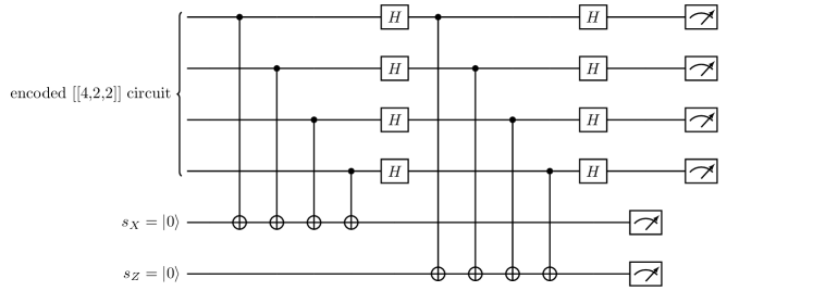
Figure 2: Syndrome measurement circuit for the [[4,2,2]] error detection code.

Since all the basis states of this encoding have even parity (even number of 1s in the physical basis), any single physical qubit bit flip error will take the state outside the logical codespace and result in a state with odd parity. As a result, a single physical qubit bit flip error will lead to a measurement of $s_{X}=1$. If the state is rotated using the Hadamard ($H^{\otimes 4}$) operation before measurement, any single physical qubit phase flip error will lead to a measurement of $s_{Z}=1$. Two physical qubit bit-flip errors take the state to another logical state and will remain undetected by the ancillas. Two physical qubit phase-flip errors can add a global phase to the state or leave the state effectively unchanged.

Another way to extract the error syndrome is by measuring all the data qubits and selecting measurements based on parity. Odd parity measurements indicate that a single qubit bit-flip error has occurred and is akin to performing the stabilizer measurement with ancilla $s_{X}$ in Figure 2. Similarly, odd parity of measurements made after rotating the state by applying the Hadamard ($H^{\otimes 4}$) operation indicate that a physical qubit phase-flip error has occurred and is equivalent to an $s_{Z}=1$ measurement in Figure 2. The advantage of this method over the stabilizer measurement is the reduction in the number of two-qubit gates for syndrome detection. The disadvantage is that the detection of errors requires a destructive measurement and only allows detection of one of the two types of errors, a physical bit flip or phase flip error.

This alternate method can be coupled with an ancilla for additional error detection during state preparation. This is applicable only to certain specific input logical states, $|\overline{00}\rangle,|\overline{0+}\rangle,|\overline{00}\rangle+|\overline{11}\rangle$ and can be used during the preparation of the Hartree-Fock initial state, $|\overline{00}\rangle$, in this study[22]. The ancilla detects physical qubit bit-flip errors during preparation of the input state while the parity check measurement described earlier enables detection of single physical qubit bit or phase flip errors.

3 Simulated Encoding Methods

In this section, we present details on the methods to encode the VQE algorithm and UCCD ansatz using the [[4,2,2]] code. We also review the methods used to simulate and post-process results for the electronic Hamiltonian of molecular hydrogen in the presence of circuit noise.

3.1 [[4,2,2]] Encoding of the UCC Ansatz

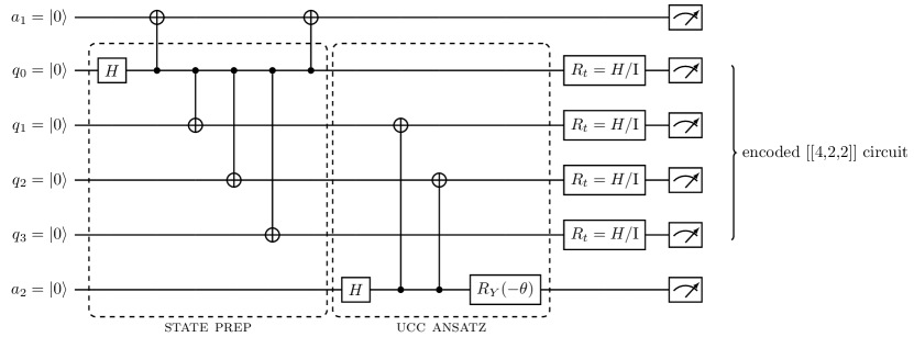
Figure 3: The [[4,2,2]] encoded ansatz for the hydrogen molecule. The block labeled ’STATE PREP’ describes the circuit to prepare the initial state in the [[4,2,2]] encoding. The block labeled ’UCC ansatz’ describes the implementation of the UCC derived hydrogen VQE ansatz in the [[4,2,2]] encoding. $R_{t}=H/I$ indicates the basis of the state prior to measurement, in the $X$ or computational basis, respectively.

We transform the two-qubit Hamiltonian in 14 into the corresponding encoded, four qubit Hamiltonian shown in 17 using the mapping in Table 1. The corresponding [[4,2,2]] encoding of the parameterized UCC two-qubit ansatz shown for simulating the hydrogen molecule is presented in Figure 3 [30]. The first block on the left, labeled “STATE PREP”, represents the circuit to prepare the initial logical $|00\rangle$ state of the unencoded ansatz and can be prepared in a wide variety of ways[22, 30, 23]. The second block labeled,“UCC Ansatz”, represents the execution of the UCC ansatz in the [[4,2,2]] encoding [30]. The parameterized rotation gate in the ansatz is non-transversal in this encoding and therefore, an ancilla, $a_{2}$, is used to teleport the gate. The final state following the action of the paramatrized unitary operator corresponding to the unencoded ($|\chi(\theta)\rangle$) and encoded circuit ($|\psi_{enc}(\theta)\rangle$) is shown in 18.

$$H_{physical}=g_{0}I+g_{1}Z_{0}Z_{1}+g_{2}Z_{0}Z_{2}+g_{3}Z_{1}Z_{2}+g_{4}X_{1}X_{2}$$ (17)

$$|\chi(\theta)\rangle =cos\frac{\theta}{2}|00\rangle+sin\frac{\theta}{2}|11\rangle$$ (18a)

$$\begin{split}|\psi_{enc}(\theta)\rangle&=\frac{1}{\sqrt{2}}[(|0\rangle_{a_{1}}\otimes(cos\frac{\theta}{2}|\overline{00}\rangle_{q_{0}-q_{3}}+sin\frac{\theta}{2}|\overline{11}\rangle_{q_{0}-q_{3}})\otimes|0\rangle_{a_{2}})\\ &+(|0\rangle_{a_{1}}\otimes(cos\frac{\theta}{2}|\overline{11}\rangle_{q_{0}-q_{3}}-sin\frac{\theta}{2}|\overline{00}\rangle_{q_{0}-q_{3}})\otimes|1\rangle_{a_{2}}))]\end{split}$$ (18b)

The action of this non-transversal gate in the encoded circuit results in a uniform superposition of equivalent states, each representing the unencoded final state, with equal probability to be in $a_{2}=|0\rangle$ or $|1\rangle$, and with each minimizing the expectation value at a different parameter. The optimal parameter, $\theta^{*}=\theta$, at $a_{2}=|0\rangle$, is shifted by $\pi$ to $\theta^{*}=\theta\pm\pi$ when $a_{2}=|1\rangle$. For the purpose of calculating expectation values, we only use outcomes with $a_{2}=|0\rangle$ resulting in the final state shown in 19. This excludes $\sim 50\%$ of the total number of outcomes measured, belonging to the subset with $a_{2}=|1\rangle$, from our calculations. The corresponding state for $a_{2}=|1\rangle$ is shown in 20.

$$\begin{split}|\psi_{enc}^{a_{2}=0}(\theta)\rangle&=\frac{(\mathbb{I}^{\otimes 5}\otimes|0\rangle\langle 0|_{a_{2}})\otimes(|\psi_{enc}(\theta)\rangle)}{\sqrt{(\langle\psi_{enc}(\theta)|0\rangle\langle 0|_{a_{2}}\psi_{enc}(\theta)\rangle)}}\\ &=|0\rangle_{a_{1}}\otimes(cos\frac{\theta}{2}|\overline{00}\rangle_{q0-q_{3}}+sin\frac{\theta}{2}|\overline{11}\rangle_{q_{0}-q_{3}})\otimes|0\rangle_{a_{2}}\end{split}$$ (19)

$$\begin{split}|\psi_{enc}^{a_{2}=1}(\theta)\rangle&=|0\rangle_{a_{1}}\otimes(cos\frac{\theta}{2}|\overline{11}\rangle_{q_{0}-q_{3}}-sin\frac{\theta}{2}|\overline{00}\rangle_{q_{0}-q_{3}})\otimes|1\rangle_{a_{2}}\end{split}$$ (20)

For expectation value calculations, since each Pauli term in the Hamiltonian in 17 is in a single basis, $X$ or $Z$, we measure the final state of the encoded ansatz in the computational basis and rotate the state using the Hadamard operation prior to measurement for the “$X_{0}X_{1}$” term. This is shown in Figure 3 as $R_{t}=H$ for the “$X_{0}X_{1}$” Pauli term or $R_{t}=I$ for terms in the computational basis, prior to measurement.

3.2 Numerical Model and Simulations

We use the XACC framework to run the numerical simulations of the VQE algorithm. XACC is a software framework for the development of hardware-agnostic programs for quantum-classical hybrid algorithms, and their implementation on near-term quantum hardware [63, 64] . We use the IBM Aer simulator within XACC for numerically simulating each ansatz and use brute force optimization by scanning 150 values of parameter $\theta\in[-\pi,\pi]$.

We model gate noise with a depolarizing error channel given as

$$\xi^{G}_{j}(\rho)=(1-p)\rho^{\prime}+p\sum_{k}\sigma^{k}_{j}\rho^{\prime}\sigma^{k}_{j}$$ (21)

where $\rho^{\prime}=G\rho G^{\dagger}$, $G$ is any single-qubit gate in the circuit acting on qubit $j$ in density matrix $\rho$, $\sigma_{j}\in\{X_{j},Y_{j},Z_{j}\}$, and $p$ is the noise parameter. Errors on a two-qubit gate acting on qubits $i$ and $j$ are modeled as $\xi^{G}_{i,j}(\rho)=\xi^{I}_{i}(\xi^{G}_{j}(\rho))$ with $I$ the identity. The noise parameter for the two-qubit gate is an order of magnitude higher than the single-qubit noise parameter as is typical in current devices. The errors resulting from this channel are single qubit errors, $E_{j}$ on qubit $j$ or two qubit errors $E_{i}\otimes E_{j}$ on qubits, $i$ and $j$ for $E_{k}\in\{X_{k},Y_{k},Z_{k},\mathbb{I}_{k}\}$.

We calculate the energy expectation values for both the unencoded and encoded simulations and for each post-selection method, using $N=2\times 10^{6}$ shots, which we determined by calculating the shot count required to estimate the energy within standard error of the mean (SEM) of 0.5mHa for a noiseless simulation. The SEM, $\sigma$, is calculated as:

$$\begin{split}\sigma_{E(\theta^{*})}&=\sqrt{\frac{var}{N}}\end{split}$$ (22)

where N is the number of shots and $var$ is the variance of the calculation. The variance is calculated as,

$$\begin{split}var&=\sum_{i}g_{i}^{2}(\langle P_{i}^{2}\rangle-\langle P_{i}\rangle^{2})\\ &=\sum_{i}g_{i}^{2}(1-\langle P_{i}\rangle^{2})\end{split}$$ (23)

where, $P_{i}$ is the $i$th Pauli term of the Hamiltonian and $g_{i}$ is the coefficient of the $i$th Pauli term. We analytically calculated the variance of the Hamiltonian to be $0.04700\ \text{Ha}^{2}$ by using the expectation value of each Pauli term in 14. We found the number of shots required to reach our target SEM of $0.5\ \text{mHa}$ as shown in 24

$$\begin{split}N&=\frac{var}{\sigma_{E(\theta^{*})}^{2}}\\ &=\frac{0.04700}{0.0005^{2}}\\ &=188000\end{split}$$ (24)

and rounded up to result in $N=2\times 10^{6}$ shots.

3.2.1 Post-Selection Strategies

We introduce and analyze several different post-selection strategies. We post-select outcomes from the measurement bitstrings once all qubits are measured. The expectation values of each Pauli term in the Hamiltonian are estimated from the available, post-selected measurements. Measurement of ancilla, $a_{1}=1$ indicates a bit flip error has occurred on qubit $q_{0}$. As a result, for post-selection by ancilla $a_{1}$ (PSA) measurement, we discard all measurements with $a_{1}=1$.

Since measurements of the encoded qubits/data qubits with odd parity indicate a single physical qubit bit or phase flip error, for post-selection by logical state parity (PSP), we discard measurement bitstrings that have odd parity but include measurement counts with both measurements of ancilla, $a_{1}=0$ and $a_{1}=1$. We also consider a post-selection strategy labeled PSAP that combines both the PSA and PSP strategies. In this post-selection method, we discard measurement outcomes that have odd parity or ancilla, $a_{1}=1$.

We also calculate the SEM for the energy estimated from each post-selection method by modifying 22 to be:

$$\sigma_{E(\theta^{*})}=\sqrt{\frac{var}{n}}$$ (25)

where $n$ is the number of samples retained after each post-selection method.

3.2.2 Probability of Success

We report on the probability of success ($\eta$) for each post-selection strategy. We define it as the fraction of samples that are retained after each post-selection method.

$$\eta=\frac{n}{N}$$ (26)

The SEM for the resulting binomial distribution for each post-selection method is calculated as

$$\sigma_{\eta}=\sqrt{\frac{(1-\eta)(\eta)}{N}}$$ (27)

where $n$ is the number of the samples after post-selection for each method, $N$ is the number of samples with $a_{2}=0$.

3.2.3 Logical Fidelity

We calculate the logical fidelity of the prepared states as generated by the noisy circuit simulations. We simulate the two-qubit UCCD ansatz state for the hydrogen molecule and the corresponding [[4,2,2]] encoded circuit described in Figure 1 and Figure 3, respectively. With the resulting final state for the encoded circuit shown in 19 we use projection operators to assess the impact of each post-selection technique using fidelity. We calculate the fidelity for the PSA method by using operators, $\Pi_{A}$, to project states from the noisy state with ancilla, $a_{1}=|0\rangle$ and identity ($\mathbb{I}$) for all other qubits. For the PSP strategy, we project states within the codespace, i.e., within the states in 16, using operators $\Pi_{P}$. And we use the operator, $\Pi_{AP}$ for projecting states with $a_{1}=|0\rangle$ and states within the codespace. The operators are shown in 28 and presented in expanded form in Appendix 7.3.

$$\Pi_{A} =|0\rangle\langle 0|_{a_{1}}\otimes|\mathbb{I}_{0}\mathbb{I}_{1}\mathbb{I}_{2}\mathbb{I}_{3}\rangle\langle\mathbb{I}_{0}\mathbb{I}_{1}\mathbb{I}_{2}\mathbb{I}_{3}|\otimes|0\rangle\langle 0|_{a_{2}=0}$$ (28a)

$$\begin{split}\Pi_{P}&=\mathbb{I}_{a_{1}}\otimes(|\overline{00}\rangle\langle\overline{00}|_{q_{0}-q_{3}}+|\overline{01}\rangle\langle\overline{01}|_{q_{0}-q_{3}}\\ &+|\overline{10}\rangle\langle\overline{10}|_{q_{0}-q_{3}}+|\overline{11}\rangle\langle\overline{11}|_{q_{0}-q_{3}})\otimes|0\rangle\langle 0|_{a_{2}=0}\end{split}$$ (28b)

$$\Pi_{AP} =\Pi_{A}\otimes\Pi_{P}$$ (28c)

We calculate the logical fidelity of the states projected using operators $\Pi_{A},\Pi_{P},\Pi_{AP}$, and the original encoded and unencoded states. We define the fidelity $F$ between two states $\rho_{1}$ and $\rho_{2}$ as

$$F(\rho_{1},\rho_{2})=(\Tr\sqrt{\sqrt{\rho_{2}}\rho_{1}\sqrt{\rho_{2}}})^{2}$$ (29)

Here, we consider the case that $\rho_{1}=|\Psi\rangle\!\langle\Psi|$, $|\Psi\rangle$ is the expected ground state, i.e., the noiseless state, from the noise-free simulation and $\rho_{2}$ is the representation of the prepared, noisy unencoded, encoded or projected state. The fidelity of the projected state, $F_{i}$, is given as:

$$F_{i}(\rho_{1},\rho_{i})=(\Tr\sqrt{\sqrt{\rho_{i}}\rho_{1}\sqrt{\rho_{i}}})^{2}$$ (30)

where $\rho_{i}=\frac{\Pi_{i}\rho_{\text{noisy}}\Pi_{i}^{\dagger}}{\Tr(\Pi_{i}\rho_{\text{noisy}}\Pi_{i}^{\dagger})}$ is the projected state, $\rho_{\text{noisy}}$ is the noisy encoded state, and $\Pi_{i}\in\{\Pi_{A},\Pi_{P},\Pi_{AP}\}$. We also calculate the minimum expectation value of energy for the state $\rho$ as

$$E(\theta^{*})=\Tr(H\rho(\theta^{*}))$$ (31)

which represents an estimate in the limit of infinite samples of the measured state.

3.2.4 Logical Errors

We define logical error ($p_{\epsilon}$) for the encoded circuit in Figure 3 as probability of any error that takes the target or ideal encoded logical state to a different encoded logical state. We restrict the calculation to states with $a_{2}=0$. Therefore the logical error is the probability of measuring any state within the codespace shown in 16 other than the state $|\psi_{enc}^{a_{2}=0}(\theta^{*})\rangle$ shown in 19.

We first calculate the probability to measure the ideal state, $p_{\text{ideal}}$, in the noisy mixed state, $\rho_{\text{noisy}}$, and the probability to measure any logical state, i.e., any state in the codespace described in 16.

$$p_{\text{ideal}} =\Tr(\rho_{\text{noisy}}\rho_{\text{ideal}})$$ (32a)

$$p_{\text{logical}} =\Tr(\Pi_{P}\rho_{\text{noisy}})$$ (32b)

From these we find the probability of any error ($p_{\epsilon_{all}}$) and probability of any non-logical error ($p_{\epsilon_{NL}}$), which is any error, single- or multi-qubit, that takes the target or ideal state, $\rho_{\text{ideal}}$, outside the codespace described in 16.

$$p_{\epsilon_{all}} =1-\Tr(\rho_{\text{noisy}}\rho_{\text{ideal}})$$ (33a)

$$p_{\epsilon_{NL}} =1-p_{\text{logical}}$$ (33b)

The probability of any logical error to occur, $p_{\epsilon_{L}}$, is then obtained by subtracting the probability of any non-logical error from the probability of any error as shown in 34.

$$\begin{split}p_{\epsilon_{L}}&=p_{\epsilon_{all}}-p_{\epsilon_{NL}}\\ &=\Tr(\rho_{\text{noisy}}\Pi_{P})-\Tr(\rho_{\text{noisy}}\rho_{\text{ideal}})\end{split}$$ (34)

We additionally calculate the impact of PSA on the logical error by replacing $\Pi_{P}$ in 32b with $\Pi_{AP}$ and find probability of logical error $p_{\epsilon_{A}}$ in this case as:

$$p_{\epsilon_{A}}=\Tr(\Pi_{AP}\rho_{\text{noisy}})-\Tr(\rho_{\text{noisy}}\rho_{\text{ideal}})$$ (35)

3.3 Circuit Error Analysis

While the errors detected by the PSP method are straightforward, in that, the method detects single physical qubit bit-flip or phase-flip error, the errors detected by the ancilla, $a_{1}$, in the PSA and PSAP methods are not as clear. We analyze the errors in this circuit construction under the standard depolarizing error model we have considered to elucidate on the errors discarded when the PSA or the PSAP method is used.

Errors under the depolarizing noise model we have considered include one- and two-qubit gate errors of the form $E_{i}$ on qubit $q_{i}$ and $E_{i}\otimes E_{j}$ on qubits $q_{i},q_{j}$, respectively. Additionally, $CNOT$ gates generate two-qubit correlated errors such as a bit-flip error on the control qubit will result in a bit-flip error in the target qubit. The effective error ($E^{^{\prime}}_{k}$) after a CNOT operation is applied on control qubit, $i$ and target qubit $j$ after an error has occurred on one of the qubits can be represented as $U_{ij}E_{k}|q_{i}q_{j}\rangle=E^{^{\prime}}_{k}U_{ij}|q_{i}q_{j}\rangle$ where $U_{ij}=CNOT_{ij}$ is the ideal operation and $E^{^{\prime}}_{k}=U_{ij}E_{k}U^{\dagger}_{ij}$ for $k\in\{i,j\}$. Multi-qubit errors of the form $E_{1}\otimes E_{2}\otimes E_{3}\otimes E_{4}$ for $E_{k}\in\{X,Y,Z\}$ may also arise from concurrent one-qubit noise processes occurring on multiple qubits or from propagation of error under the two-qubit error model.

During the [[4,2,2]] input state encoding, or the section labeled “STATE PREP” in Figure 3 and shown explicitly in Figure 4, the ancilla qubit $a_{1}$ is entangled with the data qubit $q_{0}$. Any bit-flip error $E_{0}\in\{X_{0},Y_{0}\}$ that occurs on qubit $q_{0}$, and effectively remains a bit-flip error after the last two-qubit CNOT gate from control $q_{0}$ to target $q_{3}$, labeled $E_{eff}\in\{X,Y\}$ in Figure 4, will result in a measurement outcome for ancilla $a_{1}=1$ and indicate that an error has occurred. However, a similarly occurring phase-flip error on $q_{0}$ will not impact the ancilla, $a_{1}$ and therefore, will remain undetected.

Since the “STATE PREP” section is dominated by two-qubit CNOT gates, there’s a high likelihood of two-qubit errors occurring in that section. Additionally, these errors may cascade into multi-qubit errors with each successive CNOT gate execution as represented in Figure 4. As a result, the discarding of the errors by ancilla $a_{1}$ while effected by detection of bit-flip errors on $q_{0}$, may inadvertently remove multi-qubit errors as well. Construction of the circuit such that all the CNOT gates originate at $q_{0}$ with $q_{0}$ as the control ensures that many, if not most, two-qubit errors will impact $q_{0}$. Entangling the ancilla $a_{1}$ to this qubit $q_{0}$ enables the additional detection of errors that impact more than a single qubit. Conversely, the errors that do not affect $q_{0}$ in this “STATE PREP” section will not be detected by $a_{1}$ but the likelihood of such errors is low.

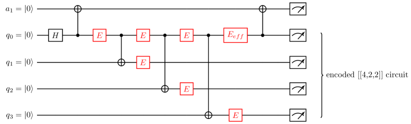
Figure 4: Logical $|\overline{00}\rangle$ state preparation circuit for error analysis. Errors, $E\in\{X,Y,Z\}$, that can occur in the input state preparation circuit, locations are representative. Ancilla $a_{1}=1$ if $E_{eff}\in\{X,Y\}$.

To verify whether the detection of error events by ancilla $a_{1}$ indeed enables multi-qubit error detection, we study the input logical state, $|\overline{00}\rangle$, prepared under the depolarizing noise channel immediately after the disentangling CNOT on the ancilla, $a_{1}$, which is the circuit labeled “STATE PREP” in Figure 1 and shown explicitly in Figure 4. We calculate the contribution towards improvement in fidelity of each post-selection method at this initial stage, when errors detected by each method are for the same final state, $|\overline{00}\rangle$, as opposed to the circuit with the UCC ansatz where the PSA method is used to detect errors during initial input state preparation and PSP at the end of the circuit. We run density matrix simulations of the circuit shown in Figure 4 for preparing the encoded logical $|\overline{00}\rangle$ state $|\phi\rangle$ shown in 36 with increasing depolarizing noise and use operators to project states similar to those in 28. Since this circuit does not include the ancilla $a_{2}$, the projection operators differ slightly and are presented in 37. We calculate the fidelity corresponding to each post-selection method by projecting states (i) with $a_{1}=|0\rangle$, (ii) within the codespace, and (iii) both within the codespace and with $a_{1}=|0\rangle$, using projection operators, $S_{A},S_{P}$, and $S_{AP}$, respectively. We use 30 to calculate fidelity, $F_{S_{i}}$, of the projected states where, in this case, $\rho_{1}=|\phi\rangle\langle\phi|$ is the noiseless state, $\rho_{i}=\frac{S_{i}\rho_{noisy}S_{i}^{\dagger}}{\Tr(S_{i}\rho_{noisy}S_{i}^{\dagger})}$ for $S_{i}\in\{S_{A},S_{P},S_{AP}\}$ are the projected states and $\rho_{noisy}$ is the noisy encoded input state.

$$\begin{split}|\phi\rangle&=|a_{1}\rangle\otimes|\overline{00}\rangle\\ &=|0\rangle\otimes\frac{1}{\sqrt{2}}(|0000\rangle+|1111\rangle)\\ \end{split}$$ (36)

$$S_{A} =|0\rangle\langle 0|_{a_{1}}\otimes|\mathbb{I}_{0}\mathbb{I}_{1}\mathbb{I}_{2}\mathbb{I}_{3}\rangle\langle\mathbb{I}_{0}\mathbb{I}_{1}\mathbb{I}_{2}\mathbb{I}_{3}|$$ (37a)

$$\begin{split}S_{P}&=\mathbb{I}_{a_{1}}\otimes(|\overline{00}\rangle\langle\overline{00}|_{q_{0}-q_{3}}+|\overline{01}\rangle\langle\overline{01}|_{q_{0}-q_{3}}\\ &+|\overline{10}\rangle\langle\overline{10}|_{q_{0}-q_{3}}+|\overline{11}\rangle\langle\overline{11}|_{q_{0}-q_{3}})\end{split}$$ (37b)

$$S_{AP} =S_{A}\otimes S_{P}$$ (37c)

The key comparison to understand the contribution of ancilla, $a_{1}$, is between the fidelity $F_{S_{P}}$ and $F_{S_{AP}}$ of states projected by $S_{P}$ and $S_{AP}$, respectively. Once the single qubit bit-flip errors are projected out of the prepared logical $|\overline{00}\rangle$ state, using $S_{P}$, any improvement in fidelity due to projection by $S_{AP}$ is entirely due to the contribution of ancilla $a_{1}$ and due to detection of multi-qubit error events.  

4 Results

The [[4,2,2]] encoded VQE circuit shown in Figure 3 and the unencoded circuit shown in Figure 1 were simulated using the IBM ‘aer’ simulator with $N=2\times 10^{6}$ shots under a standard depolarizing noise model. All qubits were measured and the measurement counts were used to calculate expectation values of the Hamiltonian for the unencoded circuit, and the encoded circuit before and after post-selection. We find the threshold of depolarizing noise at which the energy estimates fall within the chemical accuracy benchmark, present the change in energy estimates with increasing two-qubit gate noise and calculate probability of success after each post-selection strategy. We simulated the exact state for both the encoded and unencoded ansatzes using the IBM ‘aer’ density-matrix simulator to calculate the logical fidelity, and in the case of the encoded ansatz, the logical error as well. We also calculate the energy expectation values from the exact state.

The energy expectation values, variance of the calculation and probability of success at the noise parameter value at which the energy estimate reached chemical accuracy ($p=0.09\%$) are presented in Table 2. The PSAP method reaches chemical accuracy at the highest noise parameter value of $0.09\%$ than all other methods. Without post-selection, the energy of the encoded ansatz is much higher than the unencoded ansatz and the exact energy of $-1.13712$ Ha. PSA improves the energy of the encoded ansatz while still falling short of the unencoded ansatz by $0.2\%$ and PSP leads to a lower energy than PSA and the unencoded ansatz. The combined method, PSAP, leads to the highest improvement in the accuracy of the energy estimate and brings the energy estimate within chemical accuracy of $1.6$ mHa.

	Energy (mHa)	Variance (mHa)	Prob. of Success (%)
Unencoded	$-1134.81\pm 0.52$	5.38	100
Encoded No PS	$-1131.40\pm 0.72$	5.10	100
PSA	$-1132.88\pm 0.71$	4.99	$99.644\pm 0.002$
PSP	$-1134.87\pm 0.70$	4.84	$99.472\pm 0.002$
PSAP	$-1135.89\pm 0.69$	4.76	$99.232\pm 0.003$

Table 2: Comparing outcomes of the numerical simulations of the unencoded and [[4,2,2]] encoded ansatzes with and without post-selection at $0.09\%$ depolarizing noise parameter value and $N=2\times 10^{6}$ shots.

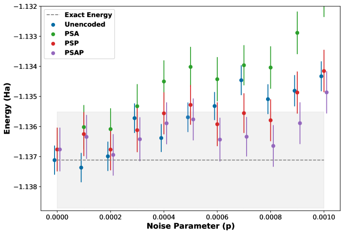
Figure 5: Estimated energy of post-selected outcomes and unencoded simulation compared against the benchmark of chemical accuracy. Shaded region represents the region of chemical accuracy and is set to $\pm 1.6$ mHa

The energy estimates from $N=2\times 10^{6}$ shots at the lower end of the noise range considered are compared against the benchmark of chemical accuracy in Figure 5 for all post-selection methods. The trends are similar to those observed in Table 2. The PSAP method is within chemical accuracy at noise parameters $\leq 0.09\%$ followed closely by the PSP method, which reaches chemical accuracy at $\leq 0.08\%$ noise. The trend continues even at larger noise values as shown in Figure 6. PSA improves the energy estimate over encoded ansatz simulation with no post-selection. However, it results in higher energy than the unencoded ansatz. PSP results in lower energy than both the encoded ansatz without post-selection and PSA. The results are also lower than the unencoded ansatz below noise level of 4%. Combining the two post-selection methods, PSAP results in the lowest energy and for all noise levels considered. Error bars in this plot of Figure 6 are too small to be visible and are in the range $0.06-2.8\ \text{mHa}$.

We also present expectation value calculations using the exact density matrix for all simulations with increasing two-qubit gate noise in Figure 6. Since calculations using the exact density matrix represent estimates of the energy in the limit of infinite shots, the energy estimate from the simulations with finite number of shots should agree with the exact density matrix calculations within some standard deviation. They are in agreement for all simulations except the calculations for the PSP and PSAP method. For both methods, energy estimated from simulations with shots is higher than calculations using the exact density matrix.

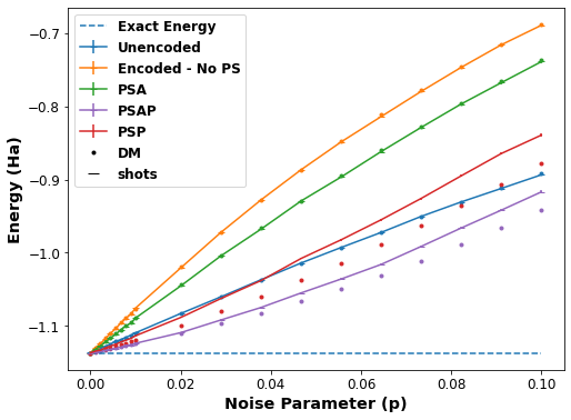
Figure 6: Energy expectation values calculated from numerical simulations of the unencoded and [[4,2,2]] encoded ansatz without (No PS) and with post-selection methods, PSA, PSP and PSAP with increasing two-qubit gate noise at 200000 shots using the IBM aer simulator and a standard depolarizing noise model.

The consequence of post-selection is having fewer samples for calculating energy expectation values. In all cases, including the noiseless case, since we are only considering half of the samples from the uniform superposition of the final state due to non-transversal rotation by ancilla $a_{2}$, i.e., only samples with $a_{2}=|0\rangle$, we start with $\sim 50\%$ of the original number of shots prior to implementation of any post-selection method due to detection of errors. We present the change in probability of success after each post-selection method with increasing noise in Figure 7, and in Table 2, for a specific noise parameter value, normalized after selecting samples with $a_{2}=|0\rangle$.

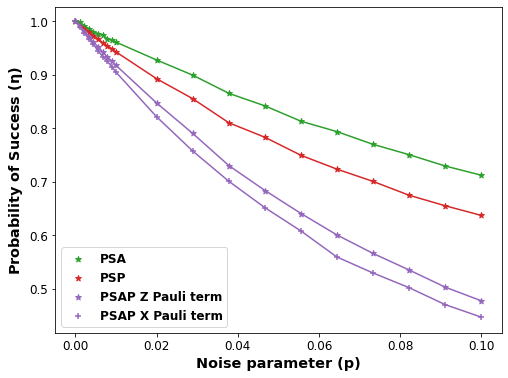
Figure 7: Probability of success of each post-selection method, PSA, PSP and PSAP of the [[4,2,2]] encoded ansatz under a standard depolarizing model. PSAP X and Z Pauli term plots are representative of the post-selection outcomes for circuits with and without the Hadamard rotation applied prior to measurement on all the encoded qubits ($q_{0}-q_{3}$) in Figure 3, respectively. Trends between the two Pauli terms are similar for all post-selection methods.

For all post-selection methods, the probability of success decreases with increasing noise indicating an increasing proportion of states with detected errors. This proportion is also determined by the method of post-selection. Post-selection by ancilla, $a_{1}=0$, measurement, PSA, retains the highest proportion of samples. However, energy expectation value calculations indicate that this does not lead to an improvement over the unencoded ansatz. Post-selection by logical state parity, PSP, results in a lower probability of success than PSA, while the highest proportion of samples are discarded due to the combined post-selection method, PSAP. Standard error of the mean in the figure are too small in magnitude to be visible but range from 0.01% (0.006% for 0.01% noise) to 0.2%. There’s also a difference in the probability of success depending on the Pauli term being measured as shown in Figure 7. Probability of success for $X$ Pauli term measurements are slightly lower than for $Z$ Pauli term measurements due to additional noise in the circuit from the Hadamard gates used to rotate the state prior to making the measurement. The PSAP $X$ and $Z$ Pauli term plots are representative and apply to all other post-selection methods.

The number of samples retained consequently impact the precision of the calculation. Table 2 shows that there is a decrease in precision/ increase in standard error of the mean of the energy estimate from the encoded simulations with and without post-selection compared to the unencoded simulation. However, the variance of the calculation for the encoded post-selected calculations are lower than the unencoded simulations and lowest for PSAP calculation, which results in the highest accuracy of the energy estimate. The decrease in the SEM, therefore, is a result of considering only half the samples with ancilla $a_{2}=0$ measurement for the encoded ansatz which is not a consideration for the unencoded ansatz, where the full $N=2\times 10^{6}$ samples are included in the SEM calculation.

We now present the logical fidelity of the the unencoded state, and the encoded state, without and with projections $\Pi_{i}\in\{\Pi_{A},\Pi_{P},\Pi_{AP}\}$ corresponding with post-selection methods PSA, PSP and PSAP, respectively, with increasing two-qubit depolarizing noise $p$ in Figure 8. The logical fidelity decreases with increasing noise, and changes with each post-selection strategy. The state fidelity of the unencoded ansatz, $F_{unenc}$, decreases with noise but is consistently better than the encoded state fidelity, $F_{enc}$ even after projecting states based on the ancilla measurement using projector $\Pi_{A}$, as indicated by fidelity, $F_{A}$. A drastic improvement in fidelity is observed for states projected using projector $\Pi_{P}$. Not only is this fidelity, $F_{P}$, higher than the fidelity, $F_{A}$, it outperforms the fidelity of the unencoded state, $F_{unenc}$, up to a noise value of $\sim 2\%$. Combining the two post-selection methods results in the best fidelity, $F_{AP}$, for this circuit and is better than $F_{unenc}$ for all noise parameters considered. Furthermore, overall decrease in fidelity of all cases with increasing noise in spite of projecting states against single- and multi-qubit errors is due to errors that go undetected in each projection, such as logical errors, introduced by the UCC ansatz or by combination of errors from state-preparation and UCC ansatz, that escaped detection by projection using $\Pi_{AP}$.

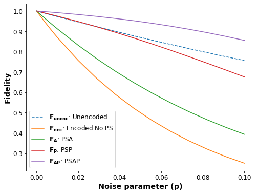
Figure 8: Fidelity of the states prepared by numerically simulating the respective unencoded state, [[4,2,2]] encoded state and projected states corresponding to the post-selection methods, PSA, PSP and PSAP, with increasing standard depolarizing noise, $p$.

Both fidelity and accuracy of the energy estimates in the simulated encoded and unencoded circuits are impacted by the errors introduced by the depolarizing error model. In the encoded circuit, in particular, the single- and two-qubit gate errors in the noise model manifest as logical, $p_{\epsilon_{L}}$ or non-logical errors ($p_{\epsilon_{NL}}$) in the final noisy mixed state. We present the proportion of logical errors, $p_{\epsilon_{L}}$, in the encoded circuit and in the projected state with $a_{1}=0$ ($p_{\epsilon_{A}}$) in Figure 9 and also present the proportion of all errors with increasing two-qubit depolarizing noise. While the errors increase with increasing noise, the proportion of all errors that are logical is much smaller. Since a logical error in this encoding requires an error event on a minimum of two qubits, the small proportion of logical errors indicate that a large proportion of errors in the encoded circuit are non-logical, single- and multi-qubit errors.

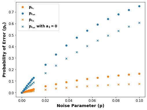
Figure 9: Probability of Error, ($p_{\epsilon}$) in the encoded circuit with increasing two-qubit depolarizing noise. Plot labeled with $a_{1}=0$ are errors in the state projected with $a_{1}=0$

We additionally calculate the logical fidelity for the encoded input state preparation circuit alone, shown in Figure 4 to study the contribution of ancilla, $a_{1}$ in the PSA and PSAP strategies to the improvement in accuracy of the energy estimate. We compare the fidelity of the state projected by $S_{P}$ with $S_{AP}$ for the same final encoded, $|\overline{00}\rangle$, input state. Improvement in fidelity, $F_{S_{P}}$, is due to the removal of states with single qubit bit-flip errors by projection operator $S_{P}$. Combining the two methods using projector $S_{AP}$ not only improves the fidelity over the fidelity $F_{S_{P}}$ for the state projected by $S_{P}$, but also results in fidelity that’s nearly 1 at $\lesssim 5\%$ noise.

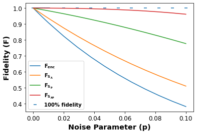
Figure 10: State fidelity for the noisy logical input $\overline{|00\rangle}$ state preparation and the projected states from the circuit labeled “State Prep” in Figure 3 and shown in Figure 4

5 Discussion

Error detection improves energy estimates over the unencoded ansatz when using post-selection by logical state parity, PSP, by itself at low noise values, and in combination with post-selection by ancilla, $a_{1}$, measurement, PSAP, at least up to $10\%$ noise. The latter also results in energy estimates within chemical accuracy at a higher noise threshold than the unencoded simulation. The magnitude of improvement in logical fidelity, $F_{P}$, of the state projected by $\Pi_{P}$, under the depolarizing noise model that we have considered, indicates that single physical qubit errors are the most probable errors and the leading cause of decrease in energy accuracy. Such single physical qubit errors can also be caused by multi-qubit errors that effectively become single qubit errors.

The decrease in precision of the estimated energy calculated from post-selected results of the simulation of the encoded ansatz compared to the unencoded ansatz is due to consideration of only one half of the results from ancilla, $a_{2}$, measurement as described in the Methods section. Within the different post-selection methods, improvement in precision is consistent with improvement in logical fidelity, indicating that in addition to improvement in the accuracy of the energy estimate, post-selection also improves the corresponding precision of the calculation. The improvement in precision in spite of increasing loss of samples with increasing accuracy of the post-selection method is a result of the improvement in variance of the calculation.

The deviation of the estimated energy using the the PSP and PSAP methods from the corresponding energy expectation value calculation using the density matrix, occurs due to the difference in order of operations between the two methods. In the latter, the states of interest are projected and the expectation value is calculated from these states. In the former, the bitstrings are post-selected from the measurement of the final state and then the expectation values are calculated from these post-selected bitstrings.

Post-selection strategies using the ancilla, $a_{1}$, lead to improvement in accuracy of the energy estimate due to detection of single and multi-qubit error events. Nearly unity fidelity, $F_{S_{AP}}$, for projecting states with logical state parity and $a_{1}=0$ measurement indicates that $a_{1}$ detects nearly all multi-qubit error events that are left undetected by projecting states with logical state parity alone. Additionally, the reduction in probability of logical errors in the state projected for ancilla, $a_{1}=0$ measurement, further confirm the detection of errors other than single qubit errors by ancilla $a_{1}$.

6 Conclusion

Post-selection based on detection of single qubit errors alone improves the accuracy of the energy estimate at low noise levels. Combining this post-selection method with post-selection using an ancilla for single and multi-qubit error detection during input state preparation further improves the accuracy of the estimate at noise levels as high as 10%. Constructing the input state-preparation circuit such that the control qubit for all the two-qubit $CNOT$ gates is the qubit, $q_{0}$, which is entagled with the ancilla, $a_{1}$, makes the detection of multi-qubit errors possible.

In addition to improvement in accuracy, post-selection also improves the precision of the calculation. Loss of precision compared to the unencoded ansatz simulation is due to the superposition of states introduced by the ancilla used to execute the VQE ansatz/sub-routine in the encoded state. Improvement in fidelity is limited by the errors, single and multi-qubit, that effectively become or remain as multi-qubit errors because they were either left undetected by the ancilla during input state preparation and/or by the parity check after the VQE sub-routine.

We have demonstrated that post-selection methods lead to an energy estimate within chemical accuracy at a higher threshold of noise than the unencoded simulation for a small two-electron system. Ansatzes for larger systems will increase the qubit and gate overhead, which will include an increase in rotation operations and potentially, parameters for optimization. Since the [[4,2,2]] code is known to be the simplest quantum error detection code, employing other error detection codes would also increase the resource cost in terms of qubits and gates. Therefore, the noise threshold at which the energy estimates reach chemical accuracy for larger systems will depend, at a minimum, on the complexity of the application circuit, the code used for error detection and the associated methods of post-selection.

7 Appendix

7.1 Hamiltonian encoding

We start with the exact electronic Hamiltonian for molecular hydrogen in second quantized form:

$$\begin{split}H(R)&=h_{00}a^{\dagger}_{0}a_{0}+h_{22}a^{\dagger}_{2}a_{2}+h_{33}a^{\dagger}_{3}a_{3}+h_{11}a^{\dagger}_{1}a_{1}\\ &+h_{2002}a^{\dagger}_{2}a^{\dagger}_{0}a_{0}a_{2}+h_{3113}a^{\dagger}_{3}a^{\dagger}_{1}a_{1}a_{3}+h_{2112}a^{\dagger}_{2}a^{\dagger}_{1}a_{1}a_{2}\\ &+h_{0330}a^{\dagger}_{0}a^{\dagger}_{3}a_{3}a_{0}+(h_{2332}-h_{2323})a^{\dagger}_{2}a^{\dagger}_{3}a_{3}a_{2}\\ &+(h_{0110}-h_{0101})a^{\dagger}_{0}a^{\dagger}_{1}a_{1}a_{0}+h_{2103}(a^{\dagger}_{2}a^{\dagger}_{1}a_{0}a_{3}+a^{\dagger}_{3}a^{\dagger}_{0}a_{1}a_{2})\\ &+h_{2013}(a^{\dagger}_{2}a^{\dagger}_{0}a_{1}a_{3}+a^{\dagger}_{3}a^{\dagger}_{1}a_{0}a_{2})\end{split}$$ (38)

The possible states within the spin-singlet configuration in the fermionic basis for the hydrogen molecule and the corresponding states in the two qubit basis are presented in Table 3. The indices correspond with those of the molecular orbitals in 7.

$|\Psi_{3}\Psi_{2}\Psi_{1}\Psi_{0}\rangle$	$|q_{1}q_{0}\rangle$
$|0101\rangle$	$|00\rangle$
$|0110\rangle$	$|01\rangle$
$|1001\rangle$	$|10\rangle$
$|1010\rangle$	$|11\rangle$

Table 3: Mapping of fermionic basis to qubit basis for all possible states of the hydrogen molecule with the spin-singlet configuration. Indices for the fermionic basis correspond with indices in 7 and indices for the qubit basis correspond with the qubits used in the circuit construction of the unitary operator.

We define the qubit excitation, de-excitation and number operators as in [37]

$$\begin{split}Q^{+}&=|1\rangle\langle 0|=\frac{1}{2}(X-iY)\\ Q^{-}&=|0\rangle\langle 1|=\frac{1}{2}(X+iY)\\ N^{(0)}&=|0\rangle\langle 0|=\frac{1}{2}(I+Z)\\ N^{(1)}&=|1\rangle\langle 1|=\frac{1}{2}(I-Z)\\ \end{split}$$ (39)

where $X$, $Y$, and $Z$ are the Pauli operators. These operators are used to construct the reduced two-qubit Hamiltonian by using the mapping presented in Table 4.

Operator	Fermionic operators	qubit operators	Pauli operators for qubits
$E_{10}$	$|0110\rangle\langle 0101|+|1010\rangle\langle 1001|$	$|01\rangle\langle 00|+|11\rangle\langle 10|$	$\frac{1}{2}(X_{0}-iY_{0})$
$E_{32}$	$|1001\rangle\langle 0101|+|1010\rangle\langle 0110|$	$|10\rangle\langle 00|+|11\rangle\langle 01|$	$\frac{1}{2}(X_{1}-iY_{1})$
$E_{00}$	$|0101\rangle\langle 0101|+|1001\rangle\langle 1001|$	$|00\rangle\langle 00|+|10\rangle\langle 10|$	$\frac{1}{2}(I+Z_{0})$
$E_{11}$	$|0110\rangle\langle 0110|+|1010\rangle\langle 1010|$	$|01\rangle\langle 01|+|11\rangle\langle 11|$	$\frac{1}{2}(I-Z_{0})$
$E_{22}$	$|0101\rangle\langle 0101|+|0110\rangle\langle 0110|$	$|00\rangle\langle 00|+|01\rangle\langle 01|$	$\frac{1}{2}(I+Z_{1})$
$E_{33}$	$|1001\rangle\langle 1001|+|1010\rangle\langle 1010|$	$|10\rangle\langle 10|+|11\rangle\langle 11|$	$\frac{1}{2}(I-Z_{1})$

Table 4: Fermionic (de)excitation and number operators mapped to the corresponding qubit and Pauli operators, where $E_{pq}$ represents the excitation and number operators when $p\neq q$ and $p=q$, respectively. The Pauli operators are constructed using 39.

The electronic Hamiltonian is then reduced as

$$\begin{split}H&=\sum_{pq}h_{pq}E_{pq}+\frac{1}{2}\sum_{pqrs}h_{pqrs}\delta_{qr}E_{ps}-E_{pr}E_{qs}\\ \end{split}$$ (40)

where $E_{pq}=a^{\dagger}_{p}a_{q}$ includes terms with $p=q$ and are presented in Table 4. Using these operators we proceed to transform the electronic Hamiltonian in 38 to a qubit representation:

$$\begin{split}H&=h_{00}E_{00}+h_{22}E_{22}+h_{33}E_{33}+h_{11}E_{11}\\ &+h_{2002}E_{22}E_{00}+h_{3113}E_{33}E_{11}+h_{2112}E_{22}E_{11}+h_{0330}E_{33}E_{00}\\ &+(h_{2332}-h_{2323})(E_{22}-E_{23}E_{32})+(h_{0110}-h_{0101})(E_{00}-E_{01}E_{10})\\ &+h_{2103}(0-E_{23}E_{10}+0-E_{32}E_{01})+h_{2013}(0-E_{23}E_{01}+0-E_{32}E_{10})\\ &=h_{00}(\frac{1}{2}(I+Z_{0}))+h_{22}(\frac{1}{2}(I+Z_{1}))+h_{33}(\frac{1}{2}(I-Z_{1}))+h_{11}\frac{1}{2}(I-Z_{0})\\ &+h_{2002}(\frac{1}{4}(I+Z_{1})(I+Z_{0}))+h_{3113}(\frac{1}{4}(I-Z_{1})(I-Z_{0}))\\ &+h_{2112}(\frac{1}{4}(I+Z_{1})(I-Z_{0}))+h_{0330}(\frac{1}{4}(I-Z_{1})(I+Z_{0}))\\ &+(h_{2332}-h_{2323})(\frac{1}{2}(I+Z_{1})-\frac{1}{4}(X_{1}+iY_{1})(X_{1}-iY_{1}))\\ &+(h_{0110}-h_{0101})(\frac{1}{2}(I+Z_{0})-\frac{1}{4}(X_{0}+iY_{0})(X_{0}-iY_{0}))\\ &+h_{2103}(-\frac{1}{4}(X_{1}+iY_{1})(X_{0}-iY_{0})-\frac{1}{4}(X_{1}-iY_{1})(X_{0}+iY_{0}))\\ &+h_{2013}(-\frac{1}{4}(X_{1}+iY_{1})(X_{0}+iY_{0})-\frac{1}{4}(X_{1}-iY_{1})(X_{0}-iY_{0}))\\ &=(h_{00}+h_{33}+\frac{h_{2002}}{4}+\frac{h_{3113}}{4}+\frac{h_{2112}}{4}+\frac{h_{0330}}{4})I\\ &+(h_{00}-h_{11}+\frac{1}{4}(h_{2002}-h_{3113}-h_{2112}+h_{0330}))Z_{0}\\ &+(h_{22}-h_{33}+\frac{1}{4}(h_{2002}-h_{3113}+h_{2112}-h_{0330}))Z_{1}\\ &+\frac{1}{4}(h_{2002}+h_{3113}-h_{2112}-h_{0330})Z_{1}Z_{0}+0+0\\ &+h_{2103}(\frac{1}{2}(-X_{1}X_{0}-Y_{1}Y_{0})\\ &+h_{2013}(\frac{1}{2}(-X_{1}X_{0}+Y_{1}Y_{0})\\ \end{split}$$ (41)

$$\begin{split}g_{0}&=h_{00}+h_{33}+\frac{h_{2002}}{4}+\frac{h_{3113}}{4}+\frac{h_{2112}}{4}+\frac{h_{0330}}{4}\\ g_{1}&=h_{00}-h_{11}+\frac{1}{4}(h_{2002}-h_{3113}-h_{2112}+h_{0330})\\ g_{2}&=h_{22}-h_{33}+\frac{1}{4}(h_{2002}-h_{3113}+h_{2112}-h_{0330})\\ g_{3}&=\frac{1}{4}(h_{2002}+h_{3113}-h_{2112}-h_{0330})\\ g_{4}&=-h_{2103}\\ \end{split}$$ (42)

Additionally:

$$\begin{split}g_{1}&=g_{2}\\ h_{2013}&=h_{2103}\\ h_{2112}&=h_{0330}\end{split}$$ (43)

This leads to the final two qubit hamiltonian shown in 8.

7.2 Unitary Operator

To transform the fermionic unitary operator to a qubit representation specific to our encoding we use qubit operators from 39. Considering only the doubles contribution in 10 and 11, we replace the fermionic operators in $T_{2}$ with qubit operators using 39 as shown in 44.

$$\begin{split}T_{2}&=\sum_{p>q\in occ.,r>s\in virt.}\theta_{rs}^{pq}(a^{\dagger}_{p}a^{\dagger}_{q}a_{r}a_{s}-a_{s}a_{r}a^{\dagger}_{q}a^{\dagger}_{p})\\ &=\theta^{20}_{31}(a^{\dagger}_{2}a^{\dagger}_{0}a_{3}a_{1}-a^{\dagger}_{1}a^{\dagger}_{3}a_{0}a_{2})\\ &=\theta^{20}_{31}(E_{10}E_{32}-E_{23}E_{01})\\ &=\theta^{20}_{31}\frac{1}{4}((X_{0}-iY_{0})(X_{1}-iY_{1}))-\frac{1}{4}((X_{1}+iY_{1})(X_{0}+iY_{0}))\\ &=\theta^{20}_{31}\frac{1}{2}(-iY_{0}X_{1}-iX_{0}Y_{1})\\ &=i\theta^{20}_{31}\frac{1}{2}(-Y_{0}X_{1}-Y_{0}X_{1}Z_{0}Z_{1})\end{split}$$ (44)

where we have used $Y_{k}Z_{k}=iX_{k}$, $X_{k}Z_{k}=-iY_{k}$, to factorize the operator in the final step. Considering our reference state $|00\rangle$, we arrive at the reduced UCC doubles ansatz as shown in 45:

$$\begin{split}U(\theta)&=e^{i\frac{\theta}{2}(-Y_{0}X_{1})}e^{i\frac{\theta}{2}(-Y_{0}X_{1}Z_{0}Z_{1})}\\ &=e^{i\frac{\theta}{2}(-Y_{0}X_{1})}e^{i\frac{\theta}{2}(-Y_{0}X_{1})}\\ &=e^{-i\theta Y_{0}X_{1}}\end{split}$$ (45)

7.3 Projection operators expanded

$$\begin{split}\Pi_{P}&=\mathbb{I}_{a_{1}}\otimes(|0000\rangle\langle 0000|+|0000\rangle\langle 1111|\\ &+|1111\rangle\langle 0000|+|1111\rangle\langle 1111|\\ &+|0011\rangle\langle 0011|+|0011\rangle\langle 1100|\\ &+|1100\rangle\langle 0011|+|1100\rangle\langle 1100|\\ &+|1010\rangle\langle 1010|+|1010\rangle\langle 0101|\\ &+|0101\rangle\langle 0101|+|0101\rangle\langle 0101|\\ &+|0110\rangle\langle 0110|+|0110\rangle\langle 1001|\\ &+|1001\rangle\langle 0110|+|1001\rangle\langle 1001|)\otimes|0\rangle\langle 0|_{a_{2}}\\ \Pi_{AP}&=|0\rangle\langle 0|_{a_{1}}\otimes(|0000\rangle\langle 0000|+|0000\rangle\langle 1111|\\ &+|1111\rangle\langle 0000|+|1111\rangle\langle 1111|\\ &+|0011\rangle\langle 0011|+|0011\rangle\langle 1100|\\ &+|1100\rangle\langle 0011|+|1100\rangle\langle 1100|\\ &+|1010\rangle\langle 1010|+|1010\rangle\langle 0101|\\ &+|0101\rangle\langle 0101|+|0101\rangle\langle 0101|\\ &+|0110\rangle\langle 0110|+|0110\rangle\langle 1001|\\ &+|1001\rangle\langle 0110|+|1001\rangle\langle 1001|)\otimes|0\rangle\langle 0|_{a_{2}}\end{split}$$ (46)

8 References

References

- [1] AI G Q 2023 Nature 614 676–681
- [2] Evered S J, Bluvstein D, Kalinowski M, Ebadi S, Manovitz T, Zhou H, Li S H, Geim A A, Wang T T, Maskara N et al. 2023 arXiv preprint arXiv:2304.05420
- [3] Yamamoto K, Duffield S, Kikuchi Y and Ramo D M 2024 Physical Review Research 6 013221
- [4] Shor P W 1995 Physical review A 52 R2493
- [5] Steane A M 1996 Physical Review Letters 77 793
- [6] Calderbank A R and Shor P W 1996 Physical Review A 54 1098
- [7] Devitt S J, Munro W J and Nemoto K 2013 Reports on Progress in Physics 76 076001
- [8] Fowler A G, Mariantoni M, Martinis J M and Cleland A N 2012 Phys. Rev. A 86(3) 032324 URL https://link.aps.org/doi/10.1103/PhysRevA.86.032324
- [9] Bravyi S, Cross A W, Gambetta J M, Maslov D, Rall P and Yoder T J 2024 High-threshold and low-overhead fault-tolerant quantum memory (Preprint 2308.07915)
- [10] Livingston W P, Blok M S, Flurin E, Dressel J, Jordan A N and Siddiqi I 2022 Nature communications 13 2307
- [11] Sivak V, Eickbusch A, Royer B, Singh S, Tsioutsios I, Ganjam S, Miano A, Brock B, Ding A, Frunzio L et al. 2023 Nature 616 50–55
- [12] Ryan-Anderson C, Bohnet J G, Lee K, Gresh D, Hankin A, Gaebler J, Francois D, Chernoguzov A, Lucchetti D, Brown N C et al. 2021 Physical Review X 11 041058
- [13] Krinner S, Lacroix N, Remm A, Di Paolo A, Genois E, Leroux C, Hellings C, Lazar S, Swiadek F, Herrmann J et al. 2022 Nature 605 669–674
- [14] Acharya R, Aleiner I, Allen R, Andersen T I, Ansmann M, Arute F, Arya K, Asfaw A, Atalaya J, Babbush R, Bacon D, Bardin J C, Basso J, Bengtsson A, Boixo S, Bortoli G, Bourassa A, Bovaird J, Brill L, Broughton M, Buckley B B, Buell D A, Burger T, Burkett B, Bushnell N, Chen Y, Chen Z, Chiaro B, Cogan J, Collins R, Conner P, Courtney W, Crook A L, Curtin B, Debroy D M, Del Toro Barba A, Demura S, Dunsworth A, Eppens D, Erickson C, Faoro L, Farhi E, Fatemi R, Flores Burgos L, Forati E, Fowler A G, Foxen B, Giang W, Gidney C, Gilboa D, Giustina M, Grajales Dau A, Gross J A, Habegger S, Hamilton M C, Harrigan M P, Harrington S D, Higgott O, Hilton J, Hoffmann M, Hong S, Huang T, Huff A, Huggins W J, Ioffe L B, Isakov S V, Iveland J, Jeffrey E, Jiang Z, Jones C, Juhas P, Kafri D, Kechedzhi K, Kelly J, Khattar T, Khezri M, Kieferová M, Kim S, Kitaev A, Klimov P V, Klots A R, Korotkov A N, Kostritsa F, Kreikebaum J M, Landhuis D, Laptev P, Lau K M, Laws L, Lee J, Lee K, Lester B J, Lill A, Liu W, Locharla A, Lucero E, Malone F D, Marshall J, Martin O, McClean J R, McCourt T, McEwen M, Megrant A, Meurer Costa B, Mi X, Miao K C, Mohseni M, Montazeri S, Morvan A, Mount E, Mruczkiewicz W, Naaman O, Neeley M, Neill C, Nersisyan A, Neven H, Newman M, Ng J H, Nguyen A, Nguyen M, Niu M Y, O’Brien T E, Opremcak A, Platt J, Petukhov A, Potter R, Pryadko L P, Quintana C, Roushan P, Rubin N C, Saei N, Sank D, Sankaragomathi K, Satzinger K J, Schurkus H F, Schuster C, Shearn M J, Shorter A, Shvarts V, Skruzny J, Smelyanskiy V, Smith W C, Sterling G, Strain D, Szalay M, Torres A, Vidal G, Villalonga B, Vollgraff Heidweiller C, White T, Xing C, Yao Z J, Yeh P, Yoo J, Young G, Zalcman A, Zhang Y, Zhu N and Google Quantum AI 2023 Nature 614 676–681 ISSN 1476-4687 URL https://doi.org/10.1038/s41586-022-05434-1
- [15] Mayer K, Ryan-Anderson C, Brown N, Durso-Sabina E, Baldwin C H, Hayes D, Dreiling J M, Foltz C, Gaebler J P, Gatterman T M, Gerber J A, Gilmore K, Gresh D, Hewitt N, Horst C V, Johansen J, Mengle T, Mills M, Moses S A, Siegfried P E, Neyenhuis B, Pino J and Stutz R 2024 Benchmarking logical three-qubit quantum Fourier transform encoded in the Steane code on a trapped-ion quantum computer arXiv:2404.08616 [quant-ph] URL http://arxiv.org/abs/2404.08616
- [16] Leung D W, Nielsen M A, Chuang I L and Yamamoto Y 1997 Physical Review A 56 2567–2573 ISSN 1050-2947, 1094-1622 URL https://link.aps.org/doi/10.1103/PhysRevA.56.2567
- [17] Knill E 2004 arXiv preprint quant-ph/0404104
- [18] Knill E 2005 Nature 434 39–44 ISSN 1476-4687 number: 7029 Publisher: Nature Publishing Group URL https://www.nature.com/articles/nature03350
- [19] Reichardt B W 2009 Algorithmica 55 517–556 ISSN 1432-0541 URL https://doi.org/10.1007/s00453-007-9069-7
- [20] Zhong Y P, Wang Z L, Martinis J M, Cleland A N, Korotkov A N and Wang H 2014 Nature Communications 5 3135 ISSN 2041-1723 number: 1 Publisher: Nature Publishing Group URL https://www.nature.com/articles/ncomms4135
- [21] Córcoles A D, Magesan E, Srinivasan S J, Cross A W, Steffen M, Gambetta J M and Chow J M 2015 Nature communications 6 6979
- [22] Gottesman D 2016 arXiv preprint arXiv:1610.03507
- [23] Vuillot C 2017 arXiv preprint arXiv:1705.08957
- [24] Linke N M, Gutierrez M, Landsman K A, Figgatt C, Debnath S, Brown K R and Monroe C 2017 Science advances 3 e1701074
- [25] Willsch D, Willsch M, Jin F, De Raedt H and Michielsen K 2018 Physical Review A 98 052348
- [26] Takita M, Cross A W, Córcoles A, Chow J M and Gambetta J M 2017 Physical Review Letters 119 180501 ISSN 0031-9007, 1079-7114 URL https://link.aps.org/doi/10.1103/PhysRevLett.119.180501
- [27] Rosenblum S, Reinhold P, Mirrahimi M, Jiang L, Frunzio L and Schoelkopf R J 2018 Science 361 266–270 publisher: American Association for the Advancement of Science URL https://www.science.org/doi/full/10.1126/science.aat3996
- [28] Roffe J, Headley D, Chancellor N, Horsman D and Kendon V 2018 Quantum Science and Technology 3 035010
- [29] Chen E H, Yoder T J, Kim Y, Sundaresan N, Srinivasan S, Li M, Córcoles A D, Cross A W and Takita M 2022 Physical Review Letters 128 110504 ISSN 0031-9007, 1079-7114 URL https://link.aps.org/doi/10.1103/PhysRevLett.128.110504
- [30] Urbanek M, Nachman B and de Jong W A 2020 Phys. Rev. A 102(2) 022427 URL https://link.aps.org/doi/10.1103/PhysRevA.102.022427
- [31] Pokharel B and Lidar D A 2024 npj Quantum Information 10 1–17 ISSN 2056-6387 publisher: Nature Publishing Group URL https://www.nature.com/articles/s41534-023-00794-6
- [32] Cao Y, Romero J, Olson J P, Degroote M, Johnson P D, Kieferová M, Kivlichan I D, Menke T, Peropadre B, Sawaya N P D, Sim S, Veis L and Aspuru-Guzik A 2019 Chemical Reviews 119 10856–10915 ISSN 0009-2665 publisher: American Chemical Society URL https://doi.org/10.1021/acs.chemrev.8b00803
- [33] Colless J I, Ramasesh V V, Dahlen D, Blok M S, McClean J R, Carter J, de Jong W A and Siddiqi I 2018 Physical Review X 8 011021 ISSN 2160-3308 arXiv:1707.06408 [quant-ph] URL http://arxiv.org/abs/1707.06408
- [34] Colless J I, Ramasesh V V, Dahlen D, Blok M S, Kimchi-Schwartz M E, McClean J R, Carter J, de Jong W A and Siddiqi I 2018 Physical Review X 8 011021
- [35] O’Malley P, Babbush R, Kivlichan I, Romero J, McClean J, Barends R, Kelly J, Roushan P, Tranter A, Ding N, Campbell B, Chen Y, Chen Z, Chiaro B, Dunsworth A, Fowler A, Jeffrey E, Lucero E, Megrant A, Mutus J, Neeley M, Neill C, Quintana C, Sank D, Vainsencher A, Wenner J, White T, Coveney P, Love P, Neven H, Aspuru-Guzik A and Martinis J 2016 Physical Review X 6 031007 ISSN 2160-3308 URL https://link.aps.org/doi/10.1103/PhysRevX.6.031007
- [36] Whitfield J D, Biamonte J and Aspuru-Guzik A 2011 Molecular Physics 109 735–750 ISSN 0026-8976, 1362-3028 arXiv:1001.3855 [physics, physics:quant-ph] URL http://arxiv.org/abs/1001.3855
- [37] Shee Y, Tsai P K, Hong C L, Cheng H C and Goan H S 2022 Physical Review Research 4 023154 ISSN 2643-1564 URL https://link.aps.org/doi/10.1103/PhysRevResearch.4.023154
- [38] Romero J, Babbush R, McClean J R, Hempel C, Love P J and Aspuru-Guzik A 2018 Quantum Science and Technology 4 014008 ISSN 2058-9565 publisher: IOP Publishing URL https://dx.doi.org/10.1088/2058-9565/aad3e4
- [39] Peruzzo A, McClean J, Shadbolt P, Yung M H, Zhou X Q, Love P J, Aspuru-Guzik A and O’Brien J L 2014 Nature Communications 5 4213 ISSN 2041-1723 number: 1 Publisher: Nature Publishing Group URL https://www.nature.com/articles/ncomms5213
- [40] Nam Y, Chen J S, Pisenti N C, Wright K, Delaney C, Maslov D, Brown K R, Allen S, Amini J M, Apisdorf J, Beck K M, Blinov A, Chaplin V, Chmielewski M, Collins C, Debnath S, Hudek K M, Ducore A M, Keesan M, Kreikemeier S M, Mizrahi J, Solomon P, Williams M, Wong-Campos J D, Moehring D, Monroe C and Kim J 2020 npj Quantum Information 6 33 ISSN 2056-6387 URL https://doi.org/10.1038/s41534-020-0259-3
- [41] Grimsley H R, Claudino D, Economou S E, Barnes E and Mayhall N J 2020 Journal of Chemical Theory and Computation 16 1–6 ISSN 1549-9618 publisher: American Chemical Society URL https://doi.org/10.1021/acs.jctc.9b01083
- [42] P B N, Chládek J, Veis L, Pittner J and Karol K 2021 Quantum Science and Technology 6 034008 ISSN 2058-9565 publisher: IOP Publishing URL https://dx.doi.org/10.1088/2058-9565/abf602
- [43] Zhang Y, Cincio L, Negre C F A, Czarnik P, Coles P J, Anisimov P M, Mniszewski S M, Tretiak S and Dub P A 2022 npj Quantum Information 8 1–10 ISSN 2056-6387 number: 1 Publisher: Nature Publishing Group URL https://www.nature.com/articles/s41534-022-00599-z
- [44] Cerezo M, Arrasmith A, Babbush R, Benjamin S C, Endo S, Fujii K, McClean J R, Mitarai K, Yuan X, Cincio L et al. 2021 Nature Reviews Physics 3 625–644
- [45] Tilly J, Chen H, Cao S, Picozzi D, Setia K, Li Y, Grant E, Wossnig L, Rungger I, Booth G H et al. 2022 Physics Reports 986 1–128
- [46] Metcalf M, Bauman N P, Kowalski K and De Jong W A 2020 Journal of chemical theory and computation 16 6165–6175
- [47] Liu J G, Zhang Y H, Wan Y and Wang L 2019 Physical Review Research 1 023025
- [48] Parrish R M, Hohenstein E G, McMahon P L and Martínez T J 2019 Physical review letters 122 230401
- [49] Zhang F, Gomes N, Berthusen N F, Orth P P, Wang C Z, Ho K M and Yao Y X 2021 Physical Review Research 3 013039
- [50] Liu X, Liu G, Zhang H K, Huang J and Wang X 2024 IEEE Transactions on Quantum Engineering
- [51] Lim H, Kang D H, Kim J, Pellow-Jarman A, McFarthing S, Pellow-Jarman R, Jeon H N, Oh B, Rhee J K K and No K T 2024 Scientific Reports 14 1–13
- [52] Park C Y 2024 APL Quantum 1
- [53] Matoušek M, Pernal K, Pavošević F and Veis L 2024 The Journal of Physical Chemistry A 128 687–698
- [54] Gowrishankar M, Wright J, Claudino D, Nguyen T, McCaskey A and Humble T S 2021 Numerical simulations of noisy variational quantum eigensolver ansatz circuits 2021 IEEE International Conference on Quantum Computing and Engineering (QCE) (IEEE) pp 155–159
- [55] Wright J, Gowrishankar M, Claudino D, Lotshaw P C, Nguyen T, McCaskey A J and Humble T S 2022 Materials Theory 6 18
- [56] Bartlett R J, Kucharski S A and Noga J 1989 Chemical physics letters 155 133–140
- [57] Taube A G and Bartlett R J 2006 International journal of quantum chemistry 106 3393–3401
- [58] Suzuki M 1993 Proceedings of the Japan Academy, Series B 69 161–166
- [59] Trotter H F 1959 Proceedings of the American Mathematical Society 10 545–551
- [60] Evangelista F A, Chan G K L and Scuseria G E 2019 The Journal of Chemical Physics 151 244112 ISSN 0021-9606 URL https://doi.org/10.1063/1.5133059
- [61] Nielsen M A and Chuang I L 2010 Quantum Computation and Quantum Information: 10th Anniversary Edition (Cambridge University Press)
- [62] Barenco A, Bennett C H, Cleve R, DiVincenzo D P, Margolus N, Shor P, Sleator T, Smolin J A and Weinfurter H 1995 Physical review A 52 3457
- [63] McCaskey A J, Lyakh D I, Dumitrescu E F, Powers S S and Humble T S 2020 Quantum Science and Technology 5 024002
- [64] ClaudinoDaniel, J M and I L 2022 ACM Transactions on Quantum Computing Publisher: ACMPUB27New York, NY URL https://dl.acm.org/doi/10.1145/3523285