CMB low multipole alignments across data releases

Abstract

Since the first data release from NASA’s Wilkinson Microwave Anisotropy Probe’s (WMAP) observations of the microwave sky, cleaned cosmic microwave background (CMB) maps thus derived were subjected to a variety of tests, to evaluate their conformity with expectations of the standard cosmological model. Specifically many peculiarities that have come to be called "anomalies" were reported that violate the Cosmological principle. These were followed until the end of WMAP’s final nine year data release and continued with the CMB maps derived from the recently concluded ESA’s Planck mission. One of the early topics of intense scrutiny is the alignment of multipoles corresponding to large angular scales of the CMB sky. In this paper, we revisit this particular anomaly and analyze this phenomenon across all data sets from WMAP and Planck to gain a better understanding of its current status and import.

1 Introduction

Cosmological principle is a foundational assumption of modern cosmology. Though it has been a simplifying assumption initially, large body of current cosmological data, particularly cosmic microwave background (CMB) observations, help us in putting this assumption to robust scrutiny. Indeed it has been the case since the release of the first year observational microwave background data from NASA’s WMAP space mission, when full-sky high resolution cleaned CMB maps were made publicly available for the first time (Bennett et al., 2003a, b).

Many analysis methods were proposed and applied to CMB anisotropies as more data became available from WMAP satellite. This lead to finding many interesting deviations from standard model expectations, specifically statistical isotropy, on large angular scales of the CMB sky with varying significances. Independent tests confirming the same and with more data, these anomalies appear to be robust, but with about $2-3\sigma$ significance, very likely owing to the cosmic variance of the low multipoles. As new full-sky CMB maps from ESA’s Planck space probe became available, many of these were found to still persist. See for example Schwarz et al. (2016); Bull et al. (2016); Aluri et al. (2022) for a review and current status of various CMB anomalies. The WMAP and Planck collaborations themselves made a dedicated analysis of these anomalies and found them to be at a similar significance, but attributed these features to chance occurences (Bennett et al., 2011; Planck Collaboration et al., 2014, 2016, 2020).

In this paper we are particularly interested in analyzing the breakdown of statistical isotropy of CMB modes in temperature data, and any preferred alignments among them. Anomalous alignments among low multipoles of CMB temperature sky has been one of the first instances of isotropy violation seen in CMB sky (de Oliveira-Costa et al., 2004; Ralston & Jain, 2004; Copi et al., 2004). It gained significant attention from the cosmology community, as it indicated a preferred direction for our universe (Schwarz et al., 2004; Bielewicz et al., 2004, 2005; Land & Magueijo, 2005; Copi et al., 2006; Abramo et al., 2006; Samal et al., 2008, 2009; Gruppuso & Gorski, 2010; Copi et al., 2015; Pinkwart & Schwarz, 2018; Oliveira et al., 2020).

Focus of our attention here is to study this low multipole alignment anomaly in all full-sky CMB temperature maps available thus far, starting with WMAP’s one year to (full) nine years of data, and Planck’s nominal, full and legacy mission data sets. In doing so we check for those multipoles that remained anomalous across all data sets, that in turn shed light on the nature and robustness of such anomalous features of CMB modes with the accumulation of data over the years. Further, studying CMB data from an entirely different mission i.e., ESA’s Planck probe, would also inform us on their (un)stability with respect to different kind of systematics.

2 Analysis Procedure

In this section, we outline the methods and statistics used in our present work to probe anisotropy of and alignments among CMB multipoles.

As mentioned before, many statistics were proposed and used to inspect these multipole alignment anomalies. In this work, we make use of the Power tensor method (Ralston & Jain, 2004) that is briefly described below.

2.1 Power tensor

As CMB photons reach us (i.e., observers) from all directions from the last scattering surface, CMB anisotropies are akin to signal on a sphere, and are thus expanded in terms of spherical harmonics, $Y_{lm}(\hat{n})$, which form a suitable basis to expand fluctuations in CMB radiation as

$$\Delta T(\hat{n})=\sum_{l=2}^{\infty}\sum_{m=-l}^{l}a_{lm}Y_{lm}(\hat{n})\,,$$ (1)

where $\hat{n}=(\theta,\phi)$, being the position co-ordiantes on a sphere. Here $\Delta T(\hat{n})$ represents CMB temperature anisotropies with monopole ($l=0$) and dipole ($l=1$) contributions removed, and $a_{lm}$ are the coefficients of expansion in spherical harmonic basis.

Power tensor (PT) is then defined as the quadratic estimator involving $a_{lm}$’s as

$$A_{ij}(l)=\frac{1}{l(l+1)(2l+1)}\sum_{mm^{\prime}m^{\prime\prime}}a^{*}_{lm}J^{i}_{mm^{\prime}}J^{j}_{m^{\prime}m^{\prime\prime}}a_{lm^{\prime\prime}}\,,$$ (2)

where $J^{i}$ and $J^{j}$ are the $(2l+1)$ dimensional angular momentum operator matrices : $\{J^{x},J^{y},J^{z}\}$. Thus $A_{ij}$ is a $3\times 3$ matrix whose eigenvalues and eigenvectors inform us of the nature of a particular multipole ‘$l$’ we are interested in. In essence, Power tensor maps the complex pattern on the sphere corresponding to a multipole ‘$l$’ of the CMB temperature anisotropies onto an ellipsoid. The (normalized) eigenvalues of the Power tensor tell us how deformed the ellipsoid is, and the direction of the largest eigenvalue can be taken to represent a preferred direction for that multipole. We refer to this as principal eigenvector (PEV). Note that the eigenvectors of the Power tensor are headless, meaning they do not represent a vector/specific direction pointed out in the sky, but only an axis.

The Power tensor in Eq. (2) is defined in such a way that, when isotropy holds, it’s expectation value is given by

$$\langle A_{ij}\rangle=\frac{C_{l}}{3}\delta_{ij}\,,$$ (3)

where $C_{l}$ is the theoretical angular power spectrum of the CMB temperature anisotropies. Thus the eigenvalues add up to the total power, $C_{l}$, in a multipole ‘$l$’. In terms of its eigenvalues and eigenvectors, the Power tensor can thus be written as

$$A_{ij}=\sum_{\alpha=1}^{3}e_{i}^{\alpha}\Lambda^{\alpha}e_{j}^{\alpha}\,,$$ (4)

where $\Lambda^{\alpha}$ and ${\bf e}^{\alpha}$ ($\alpha=1,2,3$) are its three eigenvalues and eigenvectors, and $i,j=\{1,2,3\}$ denotes the components of any of the eigenvectors, ${\bf e}^{\alpha}$.

Let us denote the normalized eigenvalues as $\lambda_{\alpha}=\Lambda_{\alpha}/(\sum_{\beta}\Lambda_{\beta})$. In order to characterize the violation of statistical isotopy of a multipole ‘$l$’, we use what is called the Power entropy defined as

$$S(l)=-\sum_{\alpha=1}^{3}\lambda_{\alpha}\ln(\lambda_{\alpha})\,.$$ (5)

When isotropy holds, all the eigenvalues ‘$\lambda_{\alpha}$’ are equal to $1/3$, statistically, as is obvious from Eq. (3). Thus the Power entorpy for a CMB mode falls in the range $0\leq S\leq\ln(3)$. The lower limit represents maximal anisotropy indicating a preferred axis given by the PEV, and the upper limit implies that the multipole is maximally isotropic with no preferred orientation. Let us further use  $\tilde{\bf e}_{l}$  to denote the PEV, eigenvector corresponding to the largest eigenvalue of the Power tensor.

In a given realization of the universe, as is ours, every multipole picks up an anisotropy axis represented by it’s PEV. But the significance of any deviation from isotropy/that preferred axis is assessed by comparing the Power entropy of a multipole in the data, $S_{\rm obs}$, with simulations incorporating the instrument properties appropriately. Simulated data, as described later on, were also analysed in the same way as real data, and Power entropy values from these simulations, {$S_{\rm sim}$}, will be compared with $S_{\rm obs}$ to compute its significance for a particular multipole.

2.2 CDF statistics for testing low-$l$ alignments

Independent of the eigenvalues of Power tensor of a particular multipole, PEVs from different multipoles can themselves be used to compare alignments among multipoles. A natural way to do so is to define the quantity ‘$1-\cos(\alpha_{ll^{\prime}})$’ as our alignment statistic where  $\tilde{\bf e}_{l}$$\cdot$ $\tilde{\bf e}_{l^{\prime}}$$=\cos(\alpha_{ll^{\prime}})$, and $\alpha_{ll^{\prime}}$ is the angular separation between the PEVs of any two multipoles $l$ and $l^{\prime}$. The statistic ‘$1-\cos(\alpha_{ll^{\prime}})$’ increases monotonically with $\alpha_{ll^{\prime}}$. Observed values of this statistic in data are compared with appropriate simulations to infer their significances.

Further, we can quantify the effective probability of finding a set of ‘$k_{*}$’ or more number of anomalous multipoles with respect to our test statistic, as observed in the data in the multipole range of our interest. This can be done by choosing a threshold $p$-value, $\mathbb{P}$, as the criteria below which we consider an observed $p$-value for the statistic to be anomalous. Here we choose $\mathbb{P}=0.05$ i.e., probability of random chance occurence of 5% or less (corresponding to a $2\sigma$ significance or better). When we find $k_{*}$ anomalous modes out of $n$ multipoles being analyzed, that have $p\leq\mathbb{P}$ when employing a particular statistic, then the cumulative binomial probability with respect to this threshold $p$-value is

$$P(n,k\geq k_{*},\mathbb{P})=\sum_{k=k_{*}}^{n}\binom{n}{k}\mathbb{P}^{k}(1-\mathbb{P})^{n-k}\,.$$ (6)

In the standard model of cosmology, cosmic microwave background temperature anisotropies are expected to be a statically isotropic Gaussian random field on a sphere. Since we are comparing alignments among randomly chosen multipoles, the statistic ‘$1-\cos\alpha_{ll^{\prime}}$’ follows a uniform distribution in the range $[0,1]$, because PEVs are headless and represent only an axis, and not a direction in the sky. Therefore, we refer to this quantity ($1-\cos\alpha_{ll^{\prime}}$) as the theoretical probability distribution function (tPDF in short). Thus tPDF in our case is, $P(x)=1$, treating “$1-\cos\alpha_{ll^{\prime}}$” as a random variable, ‘$x$’.

Correspondingly, the theoretical cumulative probability distibution function (tCDF) is $\mathcal{P}(x)=\int_{0}^{x}P(x^{\prime})dx^{\prime}=x$, up to some ‘$x$’ in the range $[0,1]$. Let $x_{i}(=1-\cos\alpha_{i}$, where $i$ stands for the combination $\{l,l^{\prime}\}$) be a set of alignment measures between any two PEVs from data or a simulated CMB map. Let the empirical cumulative probability distribution function (eCDF) be denoted by, say, $\mathcal{P}_{i}$. It is obtained by sorting the alignment measures $x_{i}$ in ascending order and assigning $\mathcal{P}_{i}=i/N$ up to some $x_{i}$, where $N$ is the size of the set $\{x_{i}\}$. Now the tCDF can be compared with eCDF from data or simulations using one of the CDF statistics such as the Kuiper statistic. It is defined as (D’Agostino & Stephens, 1986),

$$V=D_{+}+D_{-}\,,$$ (7)

where $D_{+}=\max\{\mathcal{P}_{i}-\mathcal{P}(x_{i})\}$, and $D_{-}=\max\{\mathcal{P}(x_{i})-\mathcal{P}_{i-1}\}$, each representing the maximum positive deviation of eCDF above the tCDF and maximum negative deviation of eCDF below the tCDF, respectively, in the entire range $x=[0,1]$.

In this work, we use the ‘$V$’ statistic to understand alignments between $l=2$ and rest of the low multipoles up to $l=61$ i.e., the first 60 cosmological multipoles, which is the multipole range of our present interest. We also apply the same statistic to quantify alignments between any two multipoles $l$ and $l^{\prime}$ in this multipole range, that are also expected to follow a uniform distribution in the interval $x=[0,1]$. Thus, the same $V$ statistic can be used to quantify deviation, if any, from the expected uniform distribution of alignment measure ‘$x$’ among different multipoles.

2.3 Alignment Tensor

Collective alignments over a range of multipoles can be tested using what is called Alignment tensor (Samal et al., 2008). It is constructed from principal eigenvectors ($\tilde{\bf e}_{l}$) of those modes obtained from Power tensor whose decomposition is shown in Eq. (4). Alignment tensor (AT) is defined as,

$$X_{ij}=\frac{1}{N_{l}}\sum_{l}\tilde{e}^{i}_{l}\tilde{e}^{j}_{l}\,,$$ (8)

where the sum is over the select range of multipole $l=[l_{min},l_{max}]$, and $\tilde{e}^{i}_{l}$ are the components of PEVs. AT can also be computed for a chosen set of multipoles to find their collective alignment axis. Here, $N_{l}$ is the number of multipoles whose PEVs were used in constructing the Alignment tensor.

Now, let $\zeta_{\alpha}$ and ${\bf f}_{\alpha}$ ($\alpha=1,2,3$) be the three (normalized) eigenvalues and eigenvectors of AT respectively. Further, let the eigenvector, say $\tilde{\bf f}$, corresponds to the largest eigenvalue of AT, say $\zeta_{3}$. This eigenvector $\tilde{\bf f}$ can be taken to represent the collective alignment axis for any set of multipoles, provided the Alignment entropy (AE) defined as

$$S_{X}=-\sum_{\alpha=1}^{3}\zeta_{\alpha}\ln\zeta_{\alpha}\,,$$ (9)

is significant. Similar to Power entropy, from this definition, Alignment entropy statistic varies in the range $0\leq S_{X}\leq\ln(3)$ where the lowest value, $0$, indicates perfect alignment of PEVs and the highest value, $\ln(3)\approx 1.1$, implies perfect isotropy. In the case where $S_{X}\rightarrow 0$, $\tilde{\bf f}$ indeed represents their collective alignment axis. The significance of this axis is assessed by comparing $S_{X}^{\rm obs}$ with those estimated from simulated CMB maps i.e., $\{S_{X}^{\rm sim}\}$.

3 Observational data and Simulations

In this study we analyze CMB maps cleaned using Internal Linear Combination (ILC) method from 1, 3, 5, 7 and 9 years of NASA’s Wilkinson Microwave Anisotropy Probe (WMAP) data, and SMICA cleaned CMB maps from 2015 and 2018 public data release of ESA’s Planck satellite mission. We also study cleaned CMB sky derived from Planck’s 2013 data, as explained later. WMAP data are available from Legacy Archive for Microwave Background Data Analysis (LAMBDA) and the Planck data is available from Planck Legacy Archive (PLA)

All the WMAP’s ILC (WILC) maps are provided at a pixel resolution of HEALPix  $N_{side}$=512 having a beam window given by a Gaussian smoothing kernel of full width at half maximum $(FWHM)=1^{\circ}$ (degree). WILC maps are cleaned in real (pixel) space by taking linear combinations of multi-frequency raw satellite maps such that “cosmic” microwave background signal remains untouched while (nearly) eliminating any foregrounds in the resulting cleaned CMB map (Bennett et al., 2003b; Eriksen et al., 2004). The Planck SMICA derived CMB maps also employ a similar approach but, the cleaning of raw satellite data maps from different frequency channels is performed in multipole space by taking linear combinations of their spherical harmonic coefficients (Delabrouille et al., 2003; Cardoso et al., 2008). Planck provided much higher resolution CMB maps, owing to its better detector capabilities at  $N_{side}$=2048, with a Gaussian beam of $FWHM=5^{\prime}$ (arcmin). For the sake of this analysis all the CMB maps - data and simulations - were generated or processed to have  $N_{side}$=512 and smoothing level given by a Gaussian beam with $FWHM=1^{\circ}$. Any ancillary data required, such as masks, were also generated at HEALPix  $N_{side}$=512. More details on these are provided in Appendix A.

Ideally, any cleaning procedure aims to remove the microwave foregrounds completely. However, in practice, there are still some (visible) foreground residuals present in the cleaned CMB maps thus obtained. Such residuals will lead to biased estimates for the quantities of our interest (eg. statistics being computed) from the cleaned CMB maps. In order to minimize such effects due to galactic residuals, we use a single mask obtained by combining WMAP’s 9yr kp8 mask (available at  $N_{side}$=512) and Planck’s 2018 common inpainting mask (originally provided at  $N_{side}$=2048). Since each of these masks are available at different HEALPix resolutions, they are processed as detailed in Appendix B to obtain a unified mask at HEALPix  $N_{side}$=512, with a non-zero sky fraction of  $f_{sky}$$\approx 0.929$. The mask thus obtained is shown in Fig. [1]. Those regions excised by this combination mask are inpainted using the iSAP package, which is a sparsity based technique to fill those regions of the sky omitted due to masking in a statistically consistent manner with the rest of the available sky.

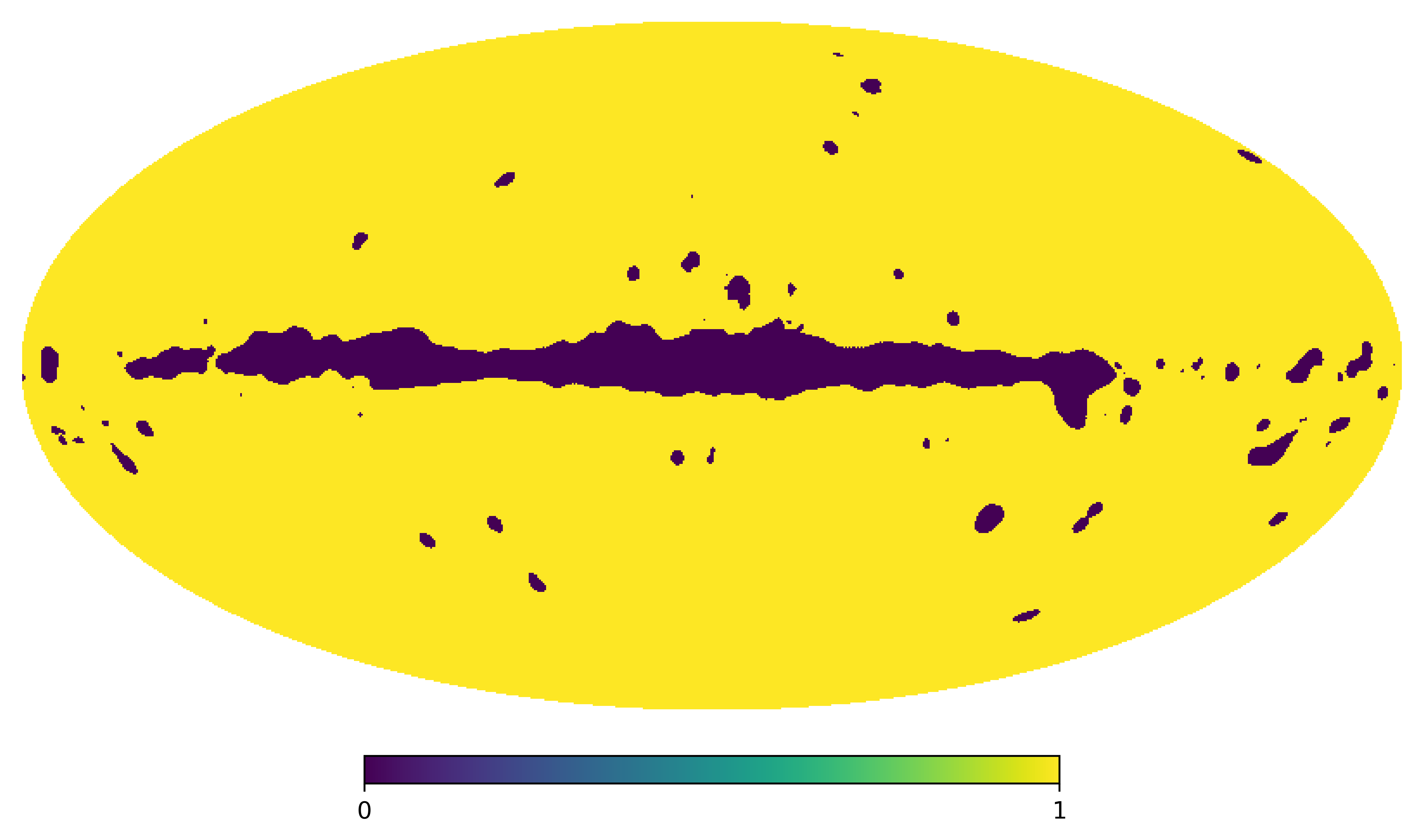
Figure 1: Unified mask obtained by merging WMAP’s 9yr kp8 mask and Planck’s 2018 common inpainting mask, both corresponding to CMB temperature data. This mask has a non-zero sky fraction of  $f_{sky}$$\approx 0.929$.

Now, in order to generate simulations corresponding to WMAP’s cleaned CMB maps viz., ILC-like CMB maps for various years, we use the weights, as published by the WMAP team in the suite of papers accompanying each data release, to combine simulated frequency specific noisy CMB maps (Bennett et al., 2003b; Hinshaw et al., 2007a; Gold et al., 2009, 2011; Bennett et al., 2013). The generation and processing of frequency specific CMB maps with appropriate beam and noise levels, to obtain mock ILC CMB maps for each of the WMAP’s data releases are explained in Appendix A.2.

Simulated CMB maps corresponding to Planck employed SMICA cleaning procedure are provided by Planck collaboration as part of each data release from Planck Legacy Archive. They are referred to as Full Focal Plane (FFP) simulations. We use the FFP SMICA CMB simulations from 2015 and 2018 data release as provided by Planck collaboration. In case of Planck 2013 data release (public release 1/PR1), corresponding simulations are currently not available as they are superseded by Full mission (2015/PR2) and Legacy data (2018/PR3) releases. Hence we process the Planck 2013 data using ILC method in pixel space, hereafter, referred to as PR1 ILC. The processing of Planck SMICA-like CMB maps from 2015 and 2018 data release, as well as the generation of PR1 ILC CMB map and corresponding simulations are described in Appendix A.1 and A.2. All these maps are then inpainted using iSAP in the same way as WMAP’s ILC maps, using the same mask shown in Fig. [1].

4 Results

4.1 Intrinisically anisotropic multipoles

First, we check for intrinsically anisotropic multipoles using the Power tensor method. The normalized eigenvalues of the Power tensor can be combined in an invariant way following Eq. (5), to identify modes that are intrinsically anisotropic. The Power entropy, $S(l)$, of the first sixty cosmological modes are computed from WMAP’s all five ILC cleaned CMB maps as released by WMAP team, and Planck’s 2013 ILC cleaned CMB map (PR1 ILC) and SMICA cleaned CMB maps from Planck’s 2015 and 2018 data releases. They are then compared with corresponding simulations. The results are shown in Fig. [2]. The solid grey line at the top of each figure indicates the maximum value $S(l)$ can take representing a completely isotropic case. The olive green line is the 95% confidence level for the Power entropy estimated from simulations for each multipole in the range of our interest $l=[2,61]$.

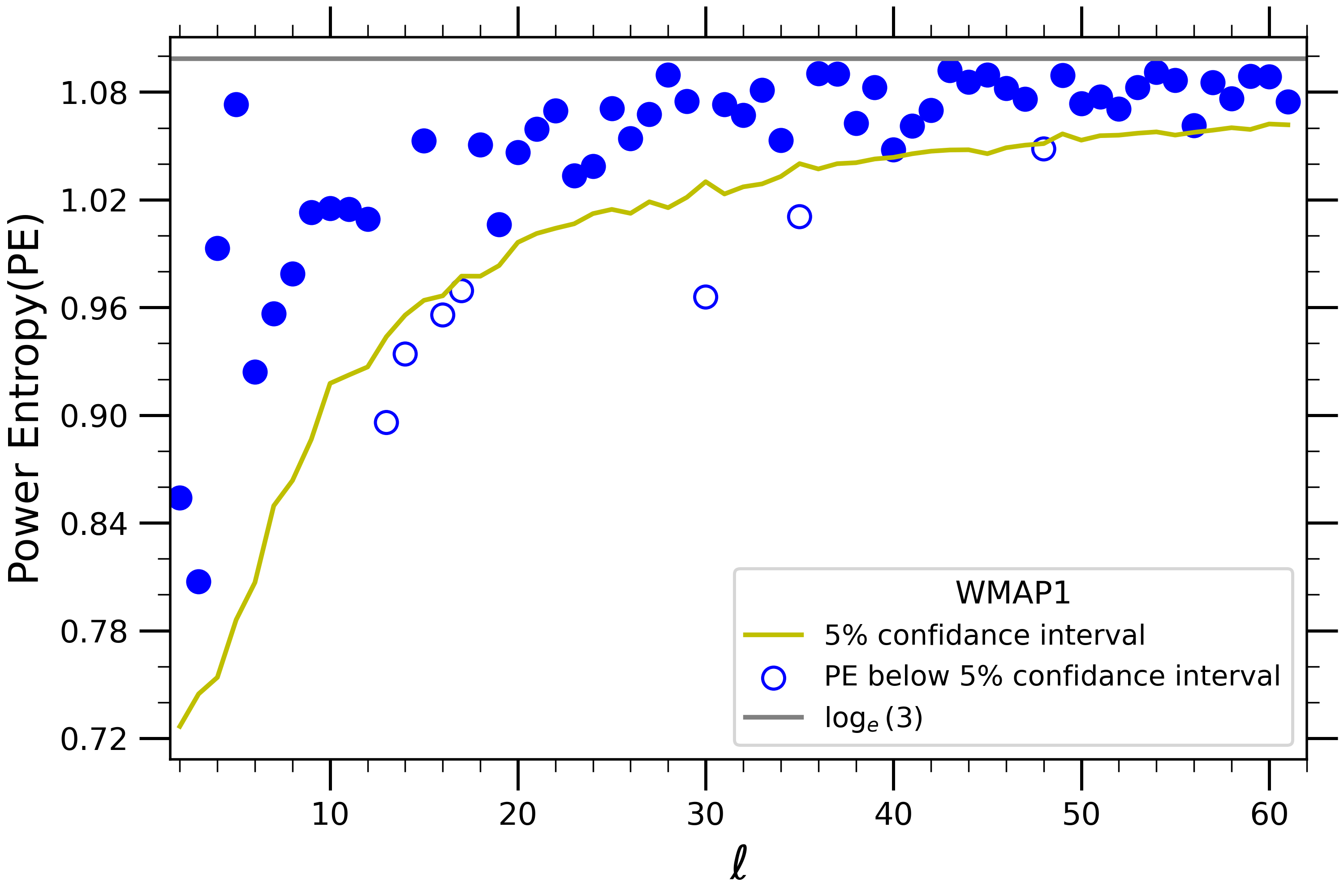
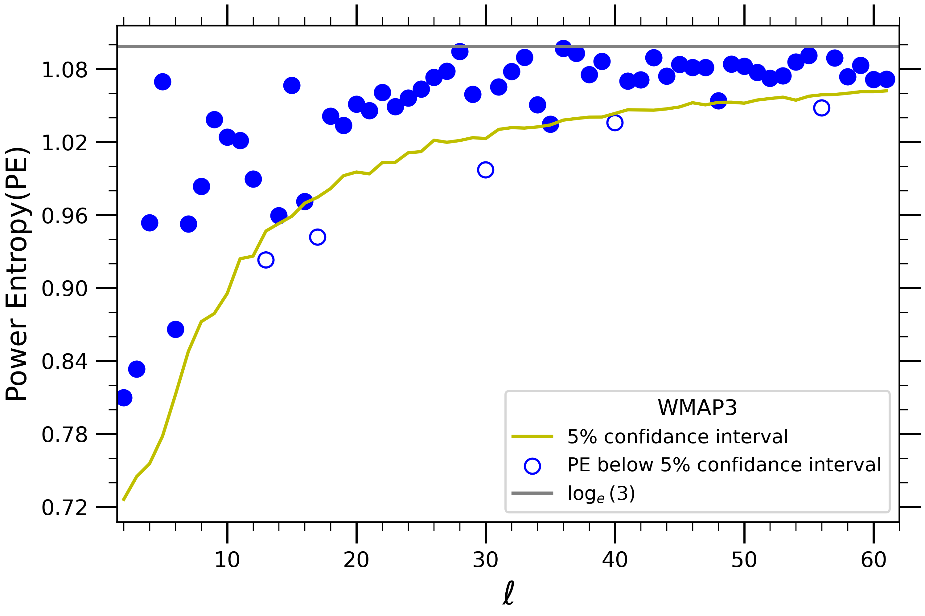
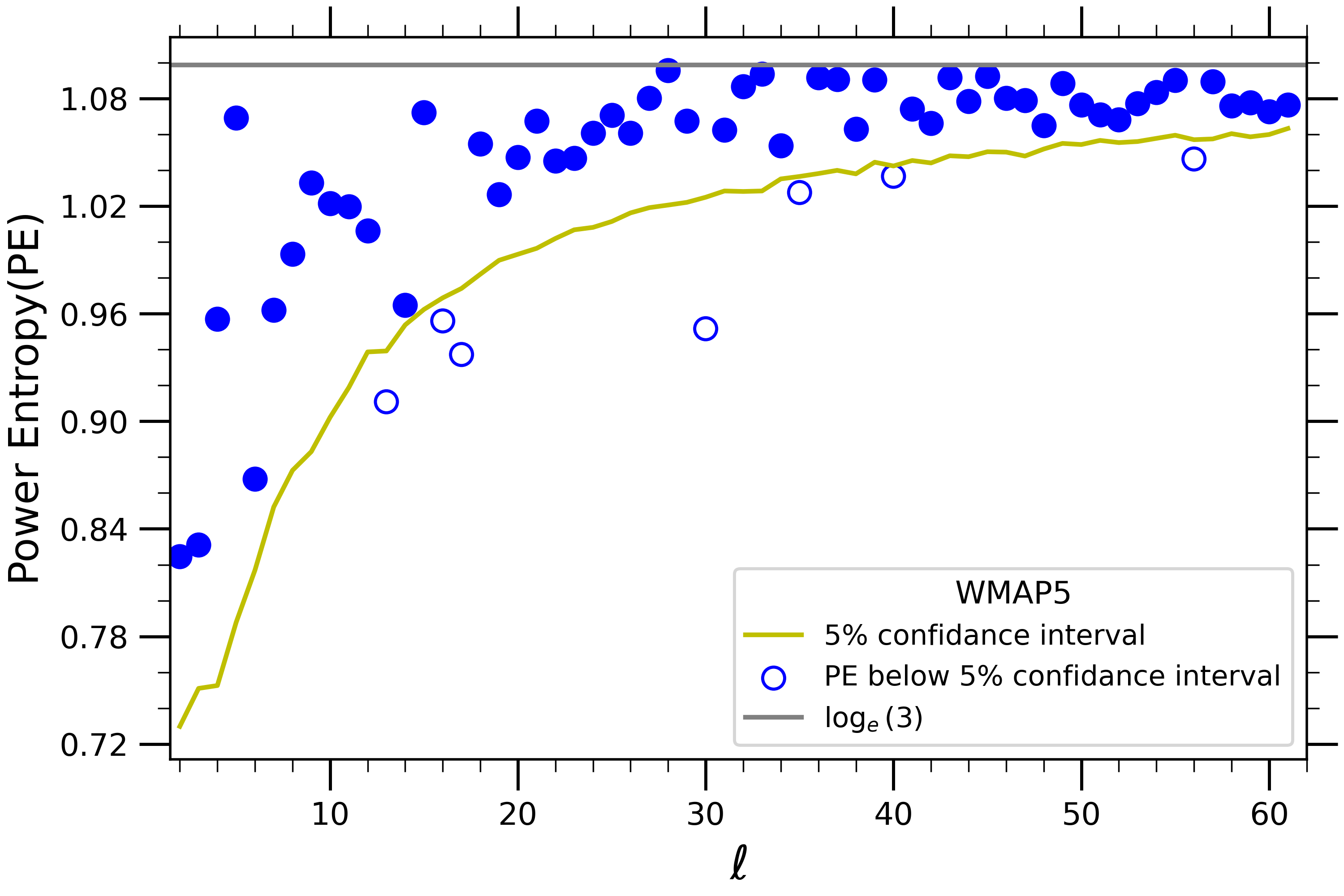
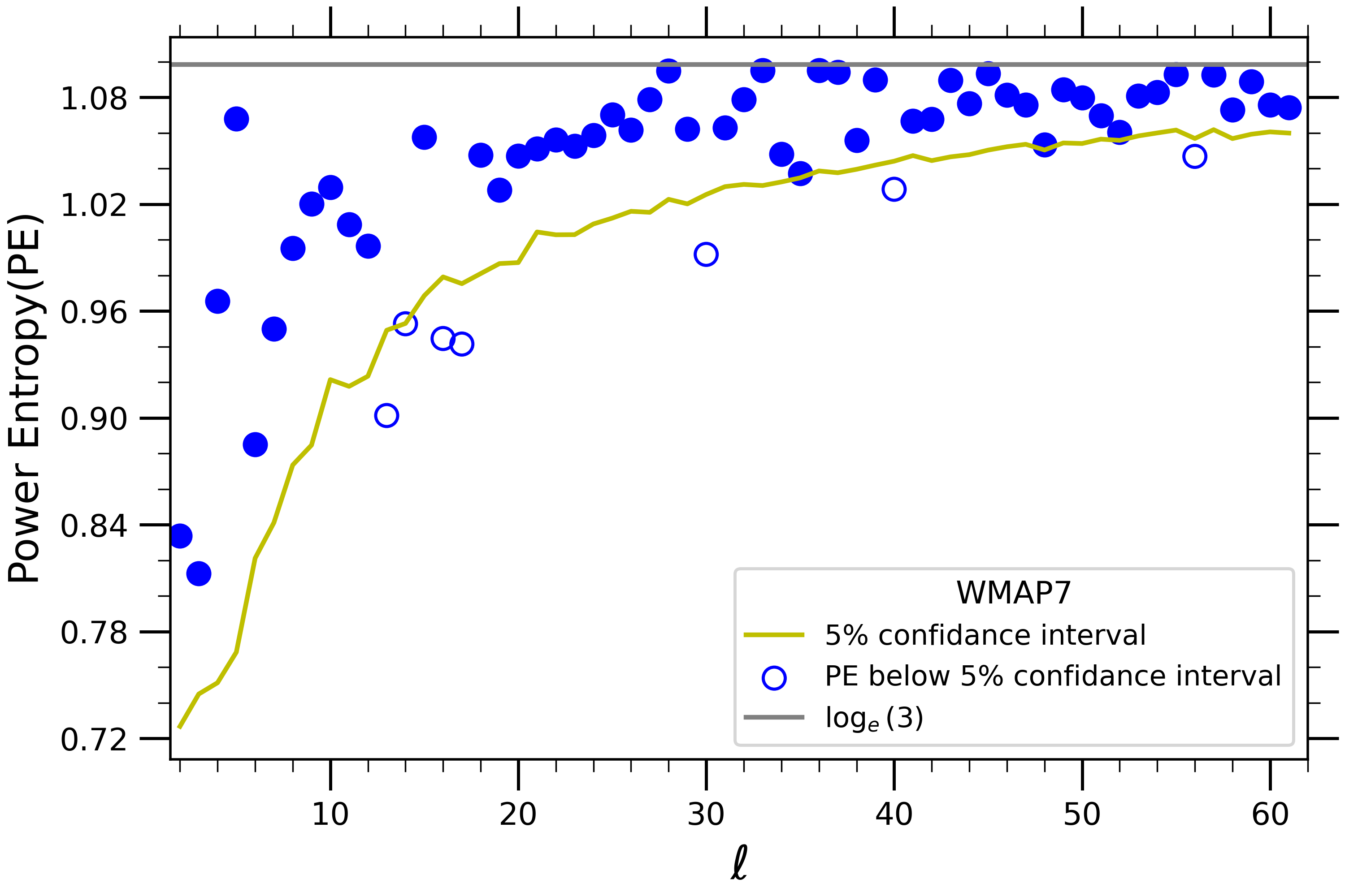
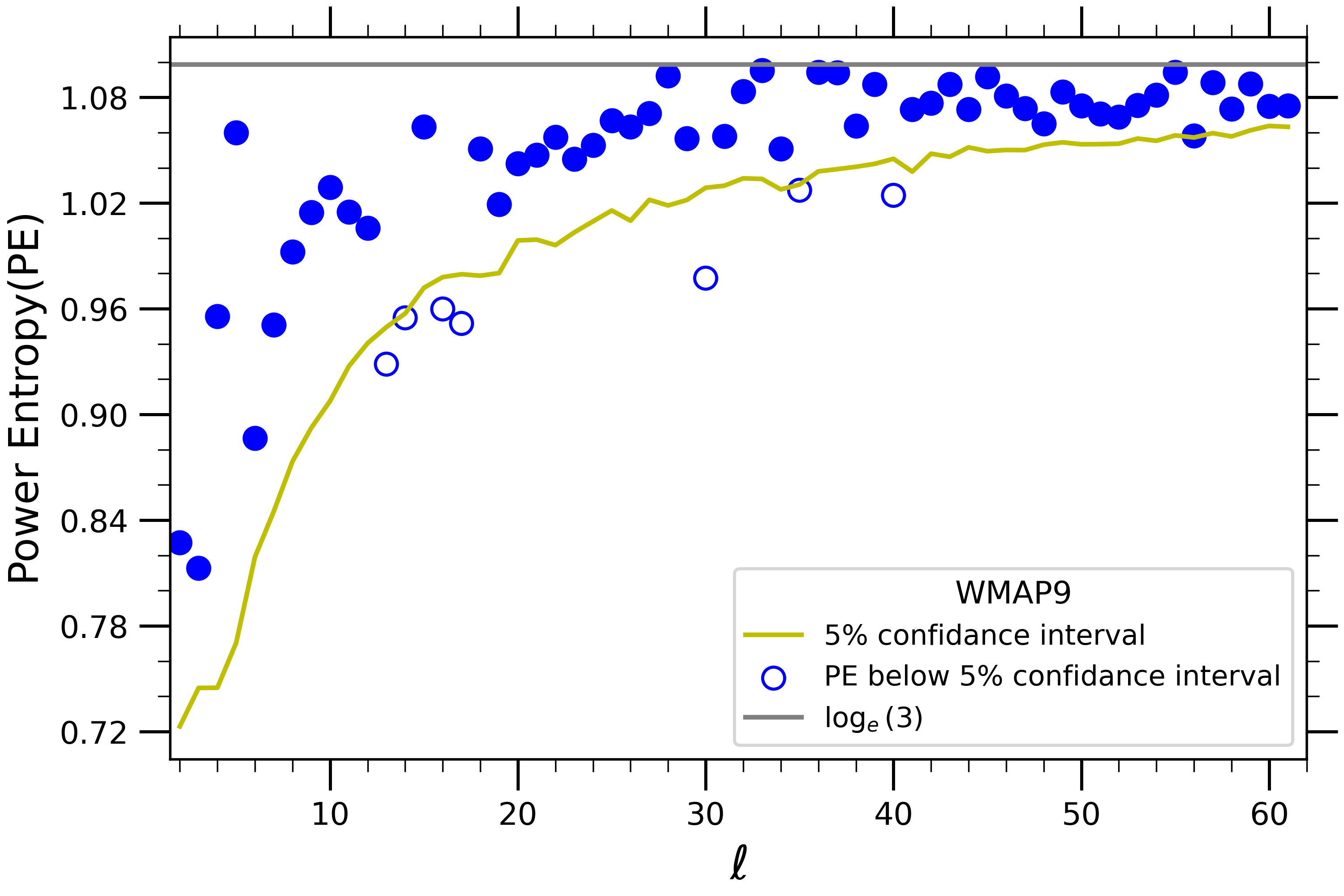
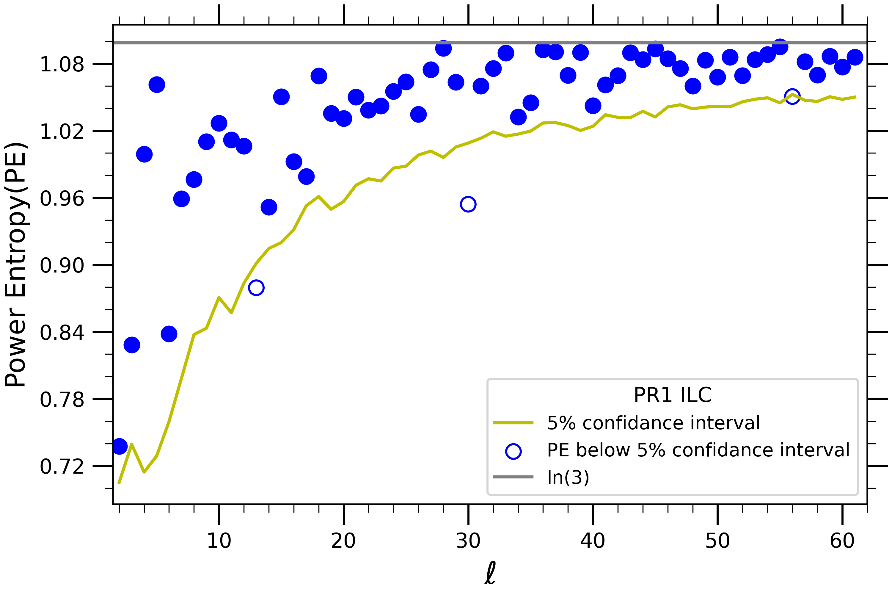
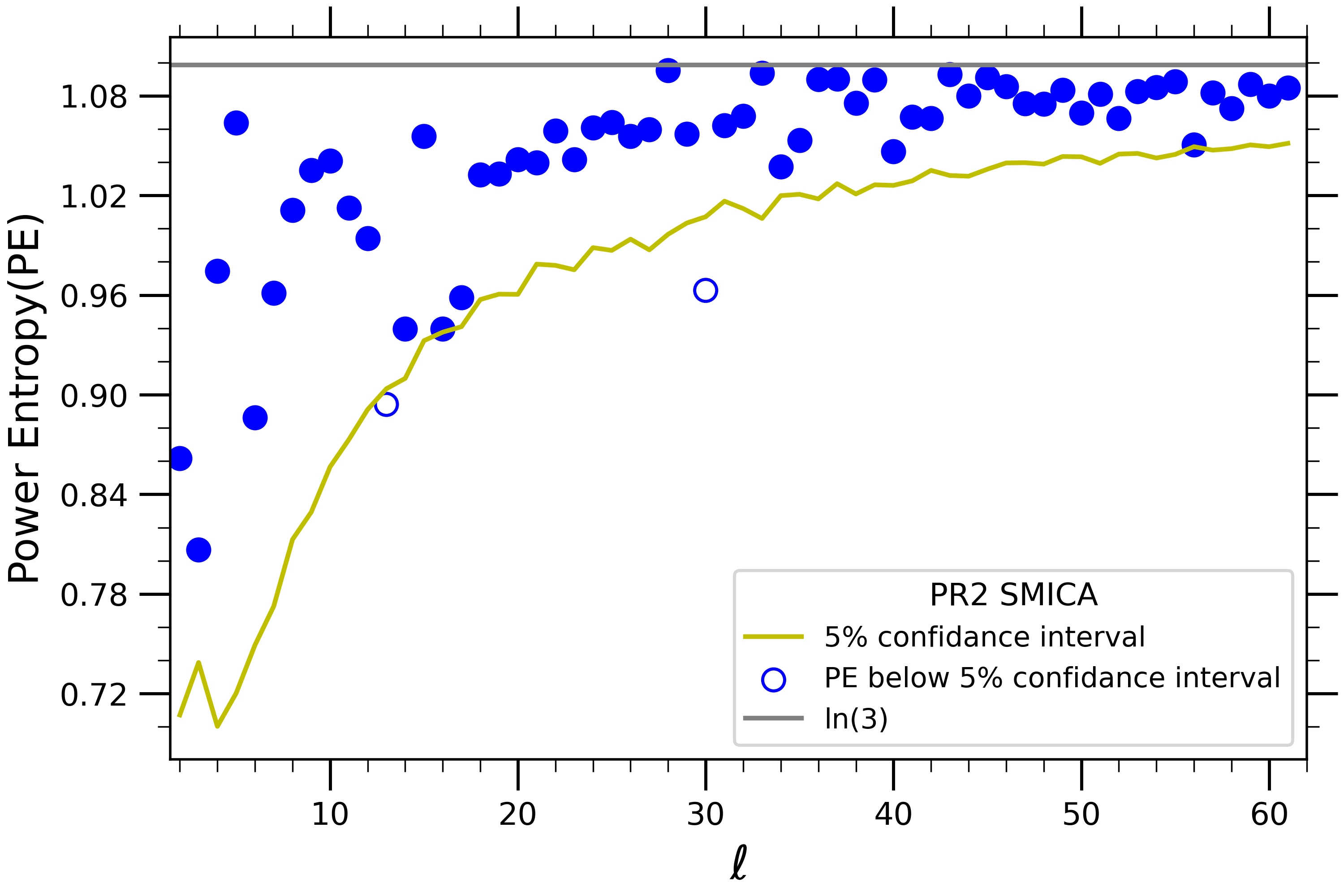
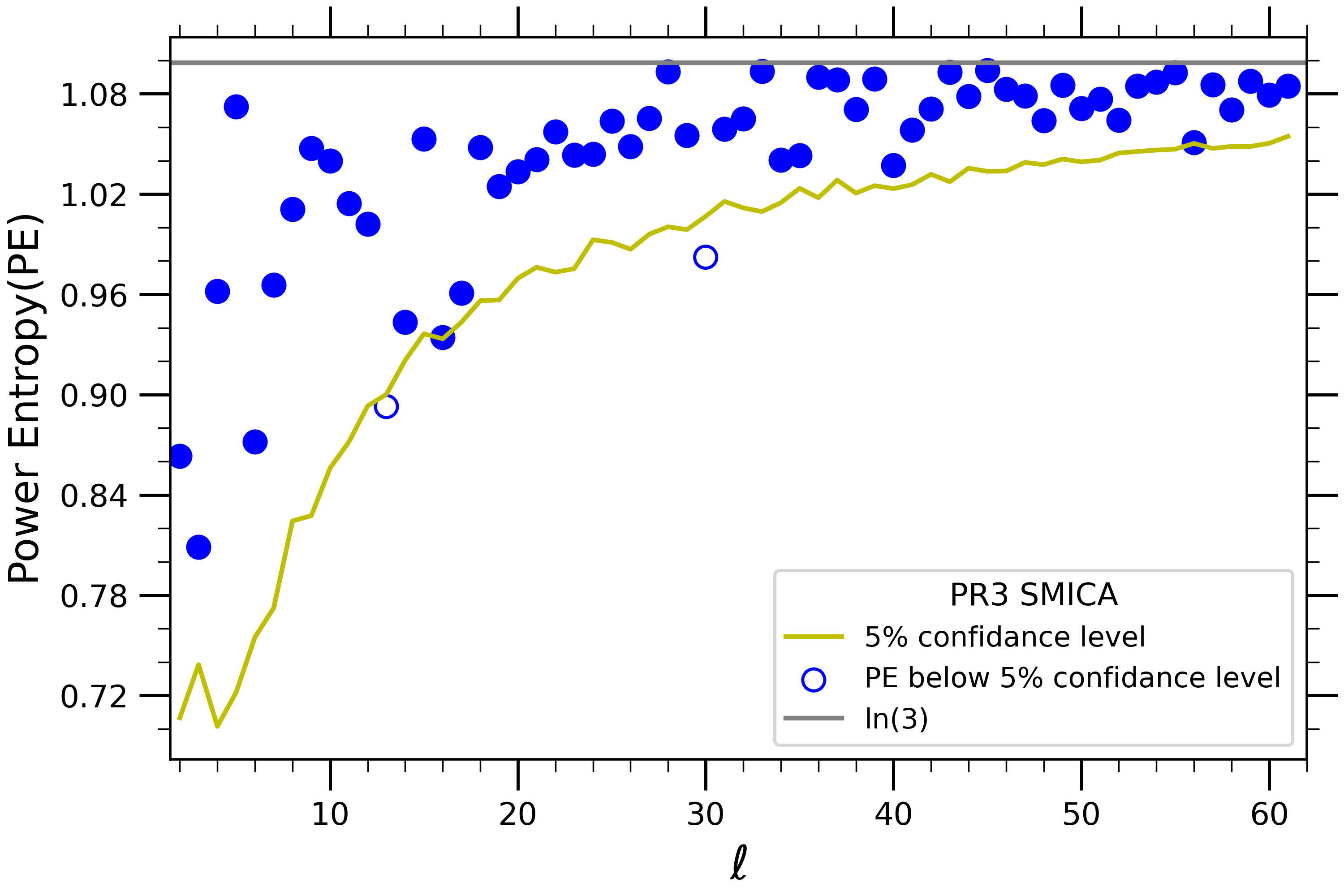
Figure 2: $p$-values of Power entropy of each multipole, ‘$S(l)$’, in CMB maps from WMAP’s obtained using Internal Linear Combination (ILC) method on 1, 3, 5, 7 and 9 years of data, as well as from Planck public release 1 data cleaned using ILC method (Planck PR1 ILC), and SMICA cleaned CMB maps from Planck’s 2015 and 2018 data releases.

Modes with anomalous Power entropy, i.e., those modes having a Power entropy with a random chance occurence probability ($p$-value) of $p\leq 0.05$ are shown as open circles, and those inside this confidence level are shown as filled circles. In Table 1, these anomalous modes are summarily listed.

Data set	Multipoles, $l$	Cumulative Bionomial
		Probability
WILC 1yr	13, 14, 16, 17,	0.030
	30, 35, 48
WILC 3yr	13, 17, 30, 40,	0.180
	56
WILC 5yr	13, 16, 17, 30,	0.030
	35, 40, 56
WILC 7yr	13, 14, 16, 17,	0.030
	30, 40, 56
WILC 9yr	13, 14, 16, 17,	0.030
	30, 35, 40
PR1 ILC	13, 30, 56	0.583
PR2 SMICA	13, 30	0.808
PR3 SMICA	13, 30	0.808

Table 1: List of multipoles whose Power entropy has a $p$-value of 5% or less, as found in WILC CMB maps from 1, 3, 5, 7 and 9 years of WMAP data, and Planck 2013 data (PR1) cleaned using ILC method, and the SMICA CMB maps from Planck probe’s 2015 and 2018 data releases. The last column denotes the cumulative binomial probability to find the observed number of anomalous multipoles or more by a random chance, whose Power entropy is anomalous with a $p$-value $\leq 0.05$, in the multipole range $l=[2,61]$.

From Table 1, we see that the multipoles $l=13$ and $30$ standout as anomalous in all the WMAP’s five ILC maps released as well as in Planck’s PR1 ILC map, and SMICA cleaned CMB maps from PR2 and PR3 data releases with a $p$-value $\leq 5\%$. So the modes $l=13$ and $30$ are intrinsically anisotropic with more power in one of it’s eigenvalues. The corresponding eigenvector - principal eigenvector (PEV) - indeed defines a preferred axis for these modes.

Last column of Table 1 indicates the cumulative probability of finding those many number of anomalous modes seen in each CMB map analyzed (as listed), from among the total number of modes analyzed (i.e., the first sixty cosmological multipoles $l=2$ to $61$). Their cumulative probability is obtained following Eq. (6). Although these modes (as listed in Table 1) violate isotropy, intrinsically, their cumulative probability is not significant when we consider the total number of modes that we studied.

4.2 Multipoles aligned with $l=2$

Here, we probe preferred alignments, if any, between the quadrupole and rest of the multipoles ($l\geq 3$). Alignment between the first two cosmological modes $l=2$ and $3$ was initially observed in CMB maps derived from WMAP 1yr data with high significance. This alignment was later found to extend to higher multipoles also (Tegmark et al., 2003; de Oliveira-Costa et al., 2004; Eriksen et al., 2004; Copi et al., 2004; Schwarz et al., 2004). Interestingly, they were also aligned with the CMB dipole and preferred axes seen in other astronomical data (Ralston & Jain, 2004).

Independent of the Power entropy, the PEVs, taken to represent an axis of anisotropy corresponding to a multipole, can be compared for any preferred alignments among them. Along with the octopole ($l=3$), that was found to be aligned with quadrupole ($l=2$) from WMAP’s first year data release, we also check it’s alignment with more (higher) multipoles in the range $l=[2,61]$. The results are presented in Fig. [3]. They depict the significance of the alignment statistic ‘$x=1-\tilde{\bf e}_{l}\cdot\tilde{\bf e}_{l^{\prime}}=1-\cos\alpha_{ll^{\prime}}$’ where $\tilde{\bf e}_{l}$ and $\tilde{\bf e}_{l^{\prime}}$ are the PEVs corresponding to the multipoles $l$ and $l^{\prime}$, and $\alpha_{ll^{\prime}}$ is the angle between them. With $l=2$, this characterizes the level of alignment between quadrupole, and rest of the multipoles $l^{\prime}=3$ to 61. A $2\sigma$ level alignment is denoted by an olive green line in each sub-plot of Fig. [3].

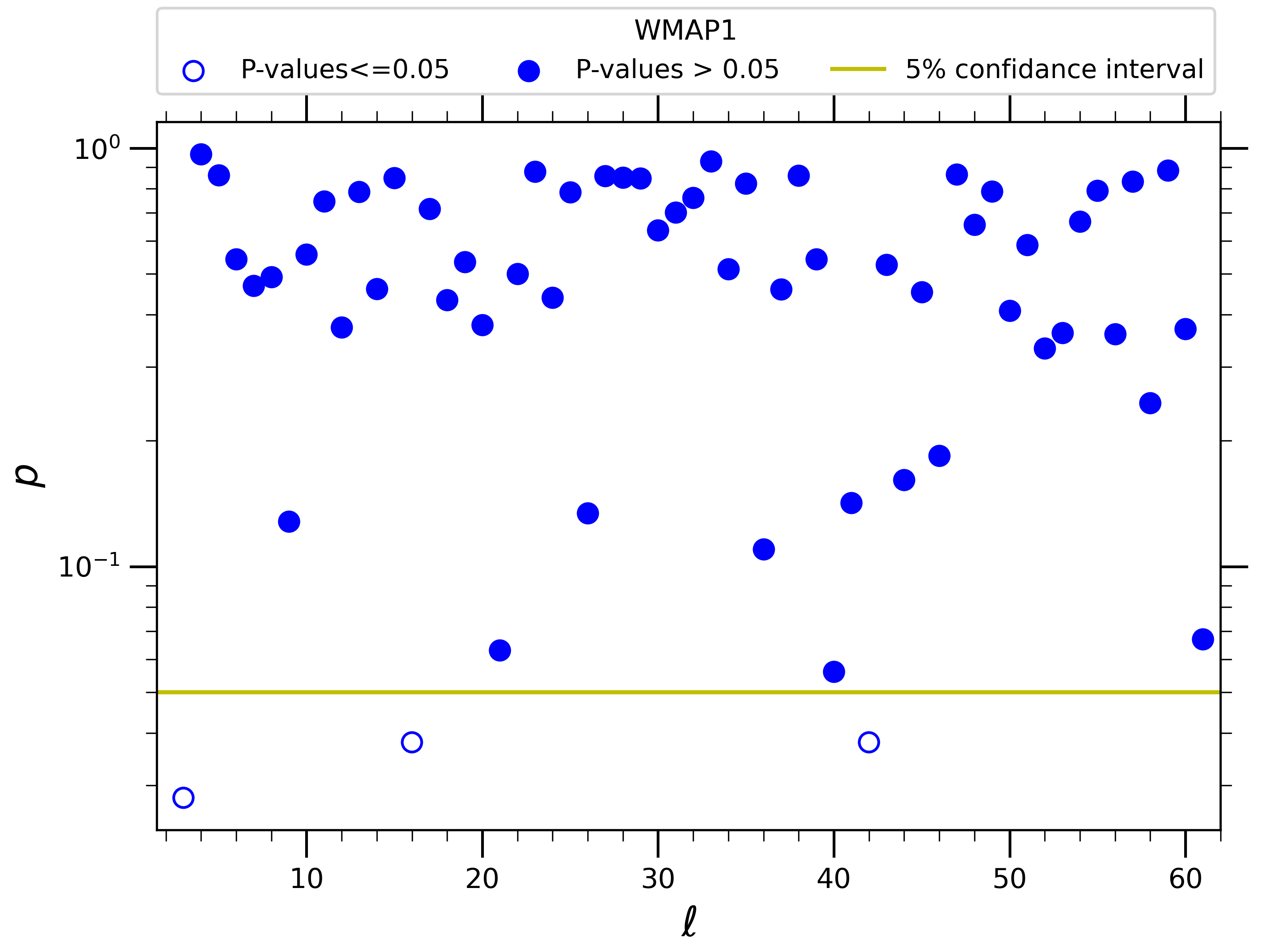
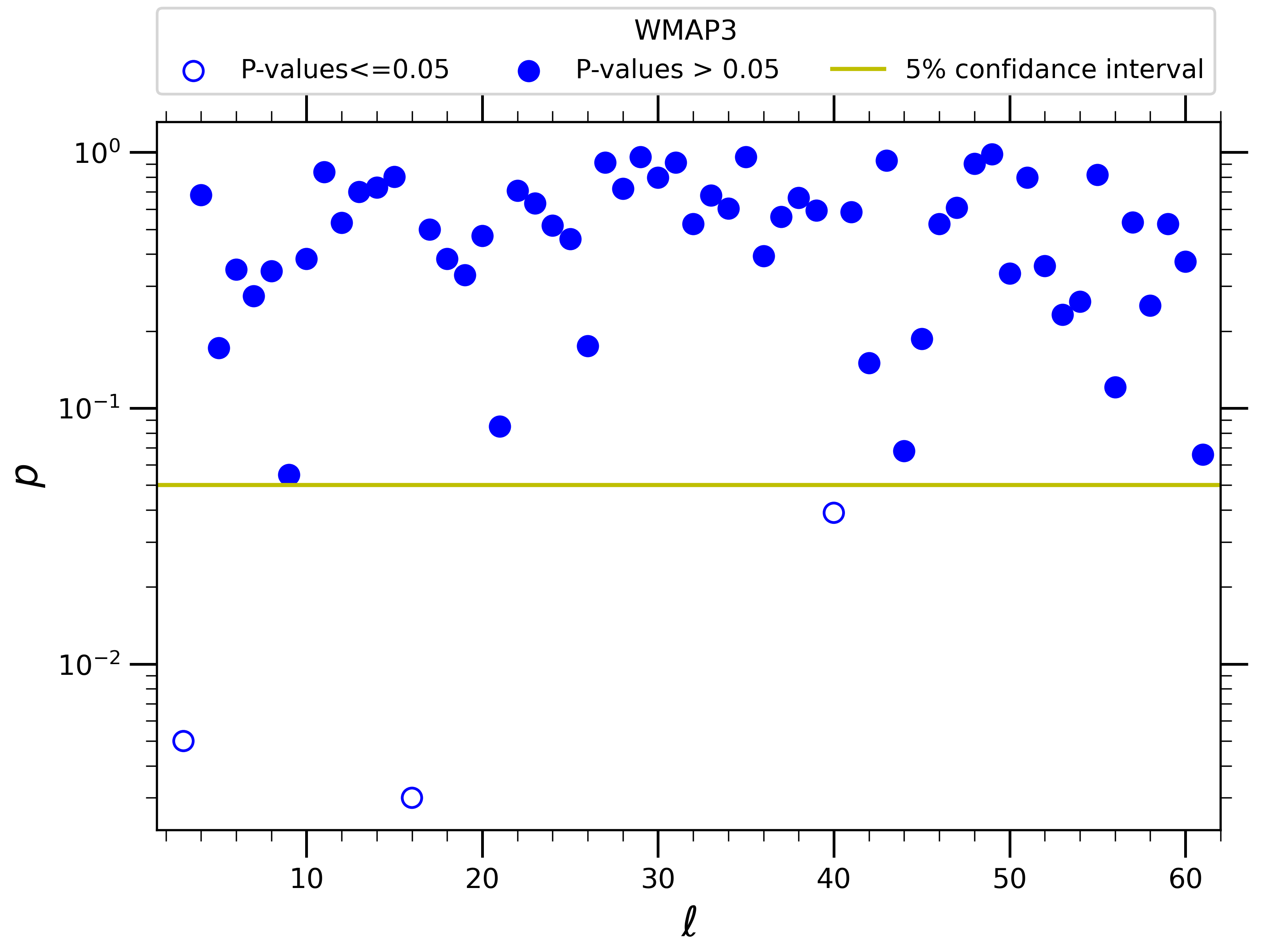
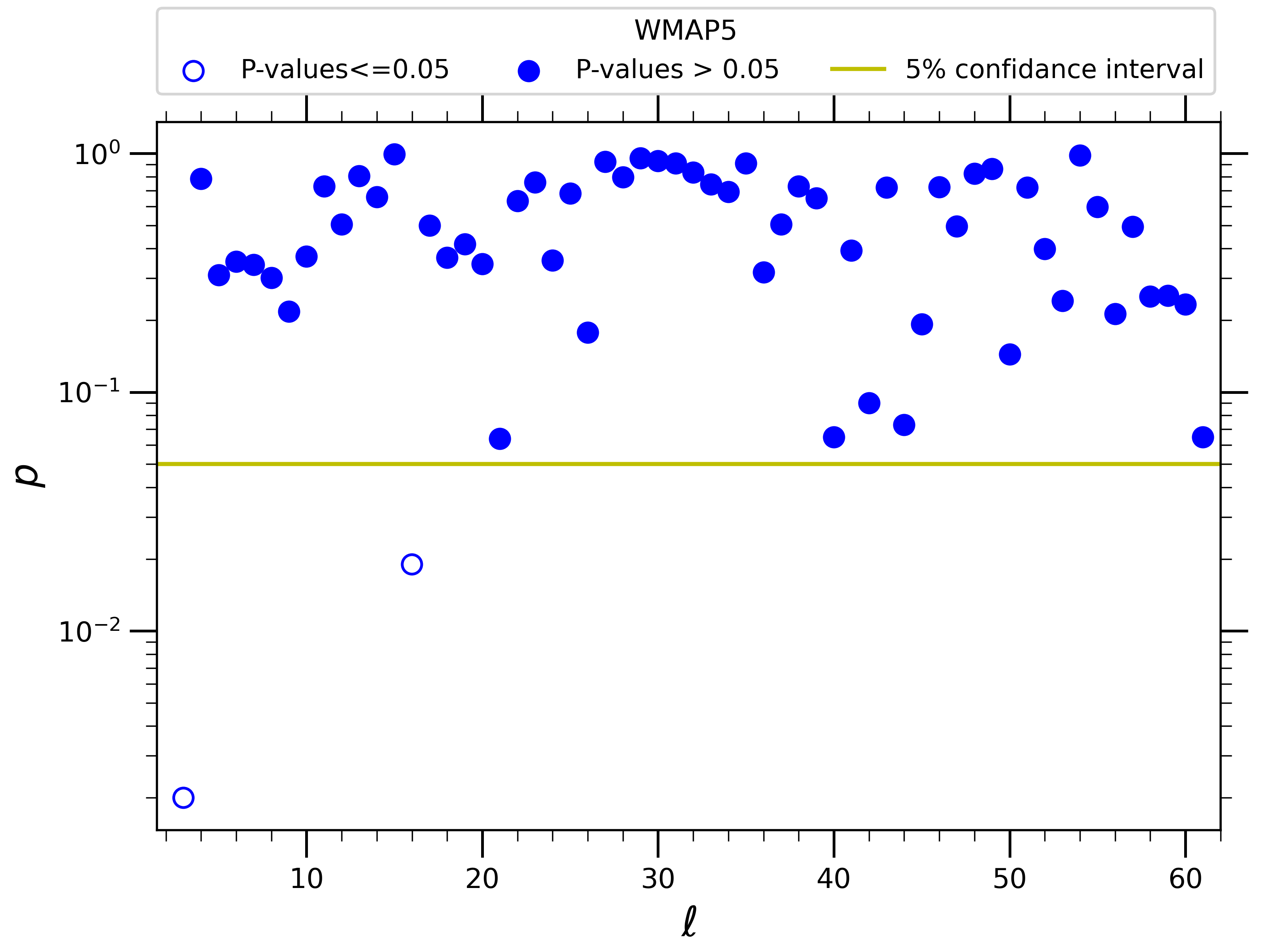
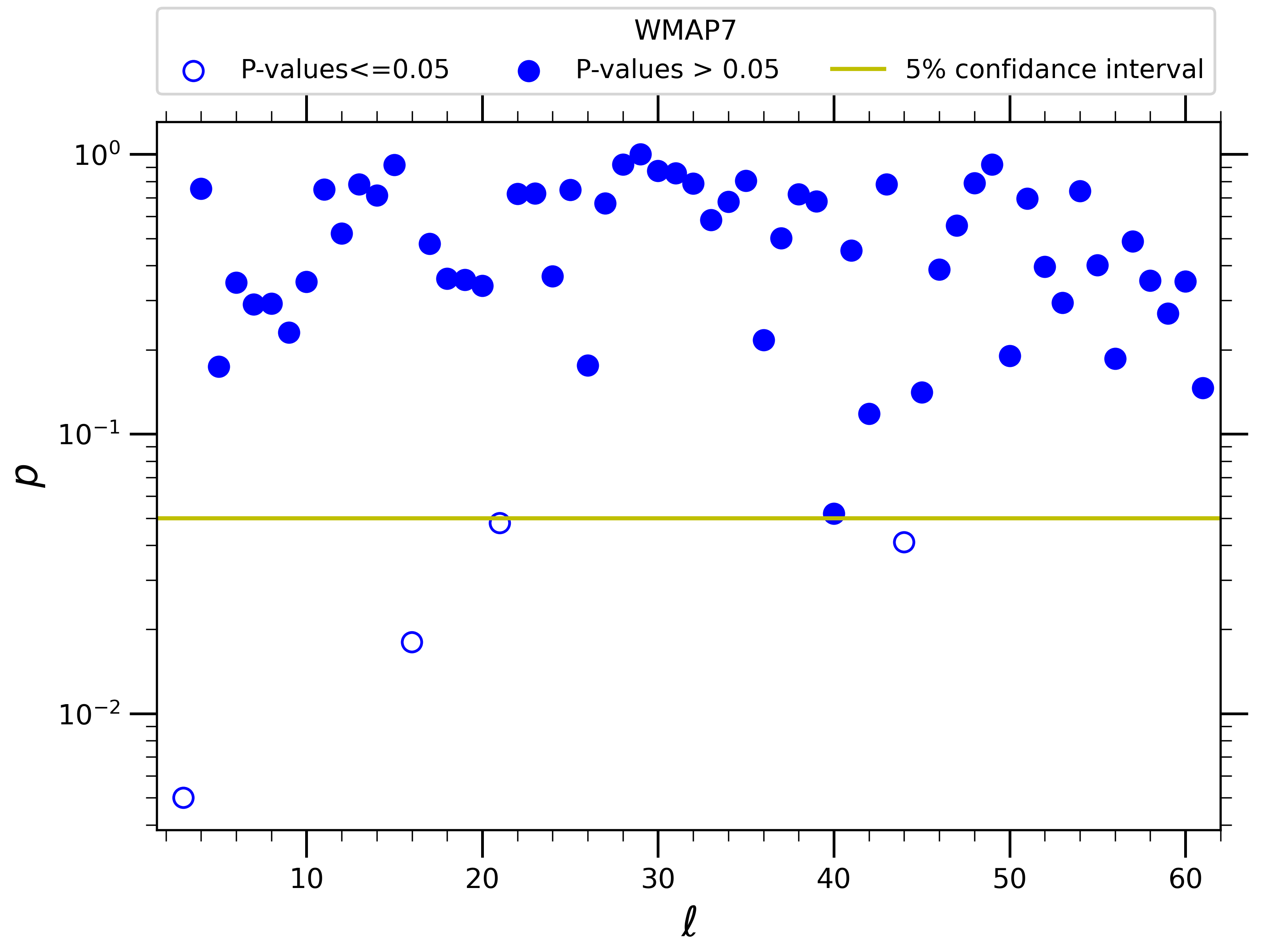
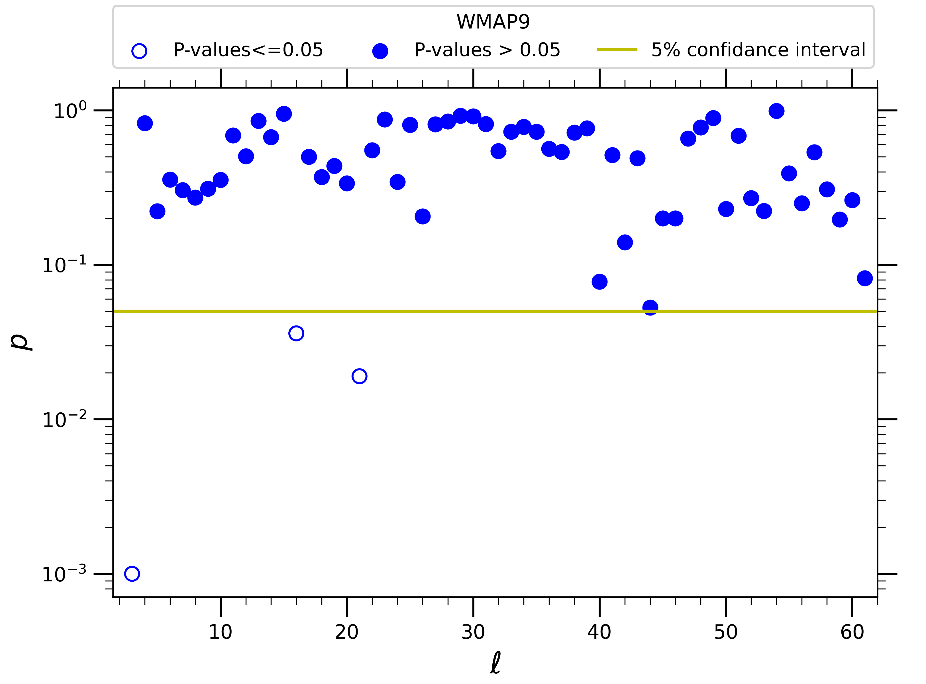
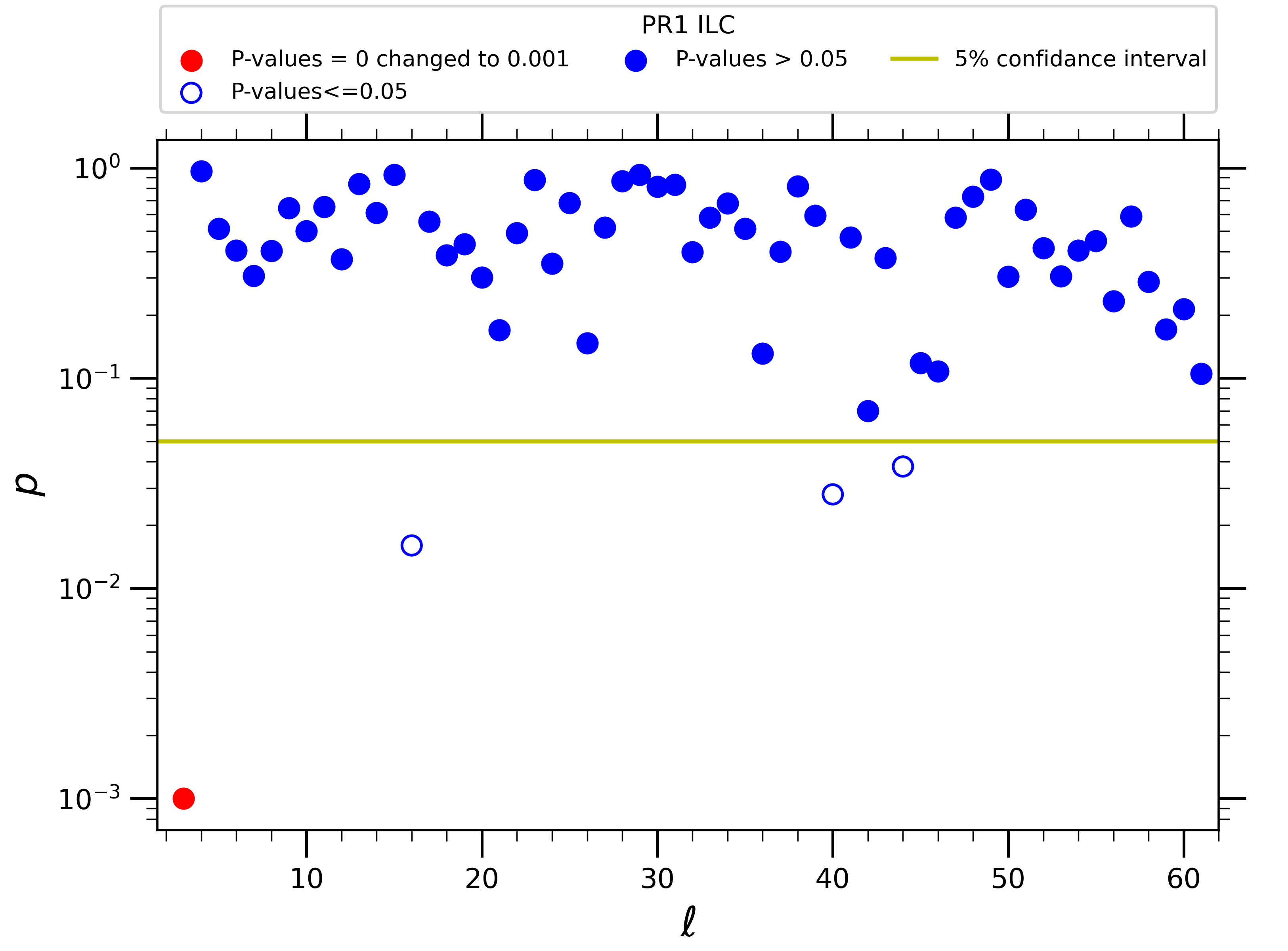
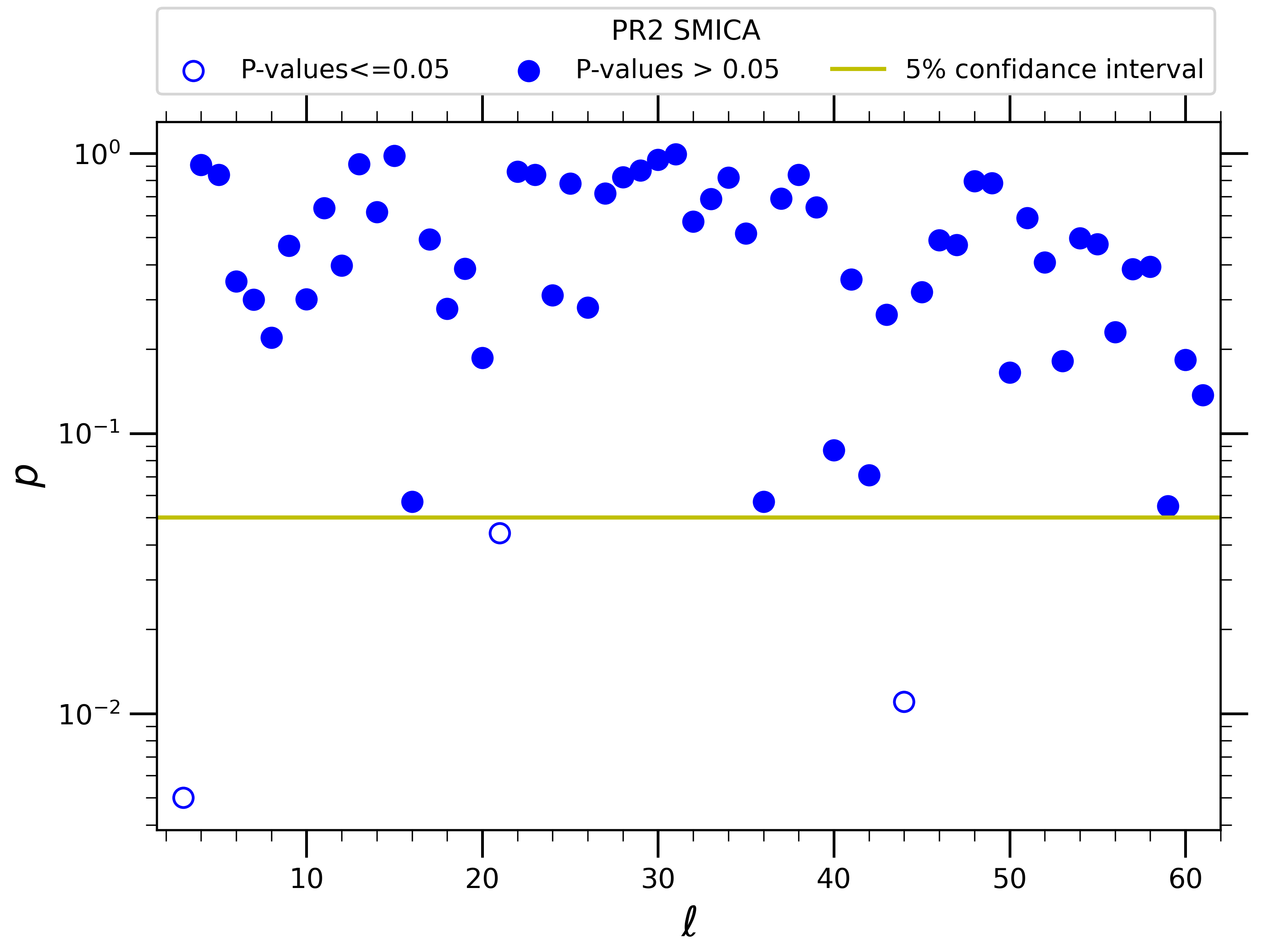
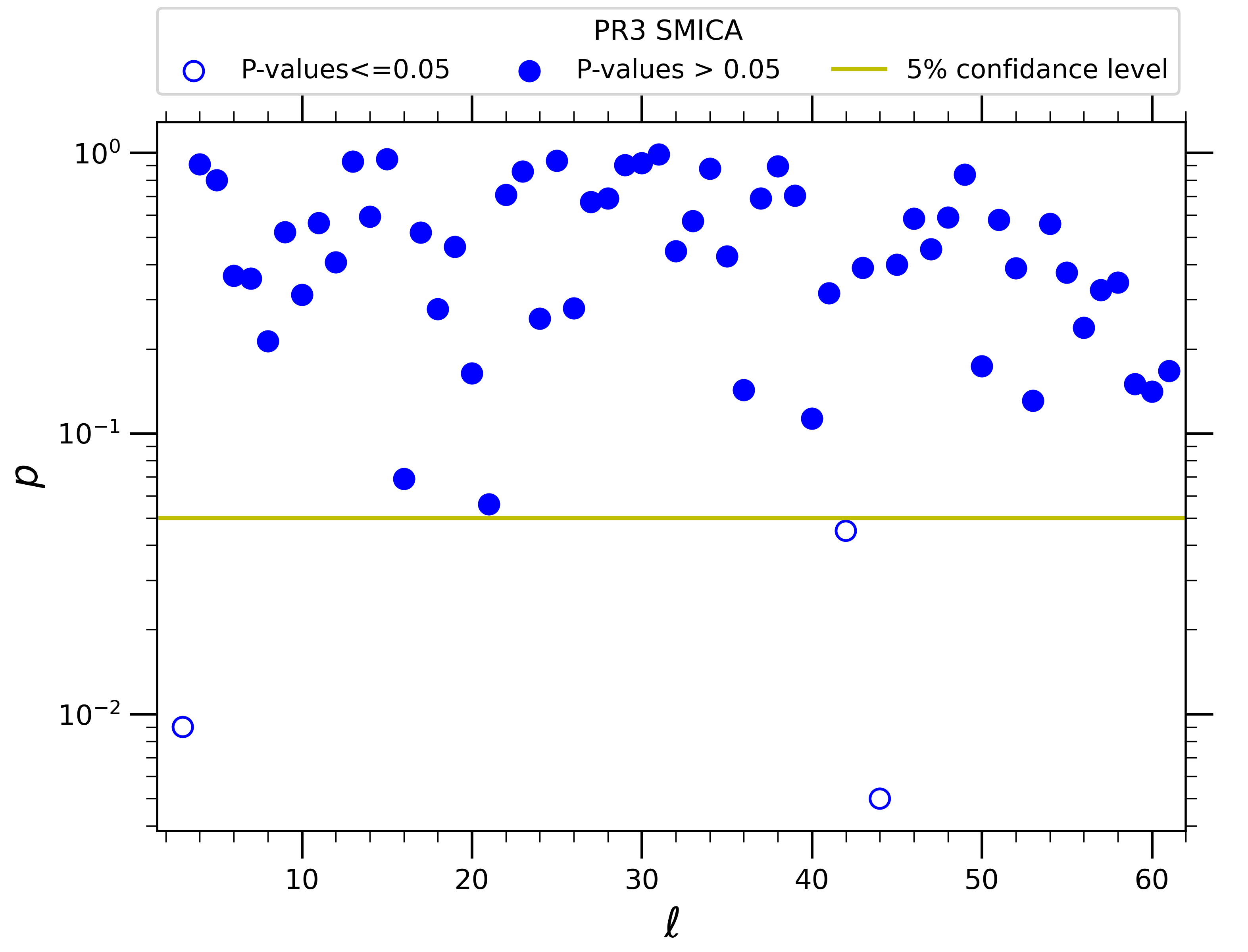
Figure 3: $p$-values corresponding to the alignment of higher order multipole PEVs with the quadrupole PEV in each CMB map from various data releases as mentioned.

From this figure, we note that the octopole mode consistently remains anomalously aligned with the quadrupole in all the CMB maps studied here. In Table 2, the set of multipoles that are anomalously aligned with the quadrupole from each data release by having a $p$-value of $\leq 0.05$ are listed in column 2.

Third column in Table 2 denotes the effective probability of finding the observed number of multipoles or more in the data to have been aligned from among the total number of modes analyzed. As it turns out this cumulative probability is insignificant. Finally in the last column of Table 2, we present the $p$-value of the Kuiper statistic defined in Eq. (7) that looks into the cumulative distribution function of the alignment measure ‘$x$’ for any deviation from isotropic distribution of PEVs with $l=2$ mode. With this CDF statistic also we don’t find significant multipole alignments in any of the CMB maps that we analyzed.

Data set	Multipoles, $l$	Cumulative	$p$-value of $V$
		Probability
WILC 1yr	3, 16, 42	0.571	0.192
WILC 3yr	3, 16, 40	0.571	0.915
WILC 5yr	3, 16	0.801	0.796
WILC 7yr	3, 16, 21, 44	0.341	0.412
WILC 9yr	3, 16, 21	0.571	0.659
PR1 ILC	3, 16, 40, 44	0.341	0.117
PR2 SMICA	3, 21, 44	0.571	0.529
PR3 SMICA	3, 42, 44	0.571	0.675

Table 2: List of multipoles that are aligned with the quadrupole with a $p$-value $\leq 5\%$ as found in CMB Internal Linear Combination (ILC) maps from all of WMAP’s five data releases, ILC cleaned Planck PR1 data, and the SMICA cleaned CMB maps from Planck probe’s 2015 and 2018 data releases. The third column denotes the cumulative probability of finding the observed number of anomalous modes or more, that have a probability of $p\leq 0.05$ as seen in each cleaned map listed in the first column. The fourth column gives the probability of the observed Kuiper statistic (V) for the mulipole alignments’ CDF from data, when compared with simulations.

4.3 Pairwise alignments among low multipoles

Now, we widen the scope of testing anisotropy as studied so far, by probing the presence of any spurious alignments among various multipoles, not just limiting to $l=2$ and the rest. The results are presented in Fig. [4] and [5].

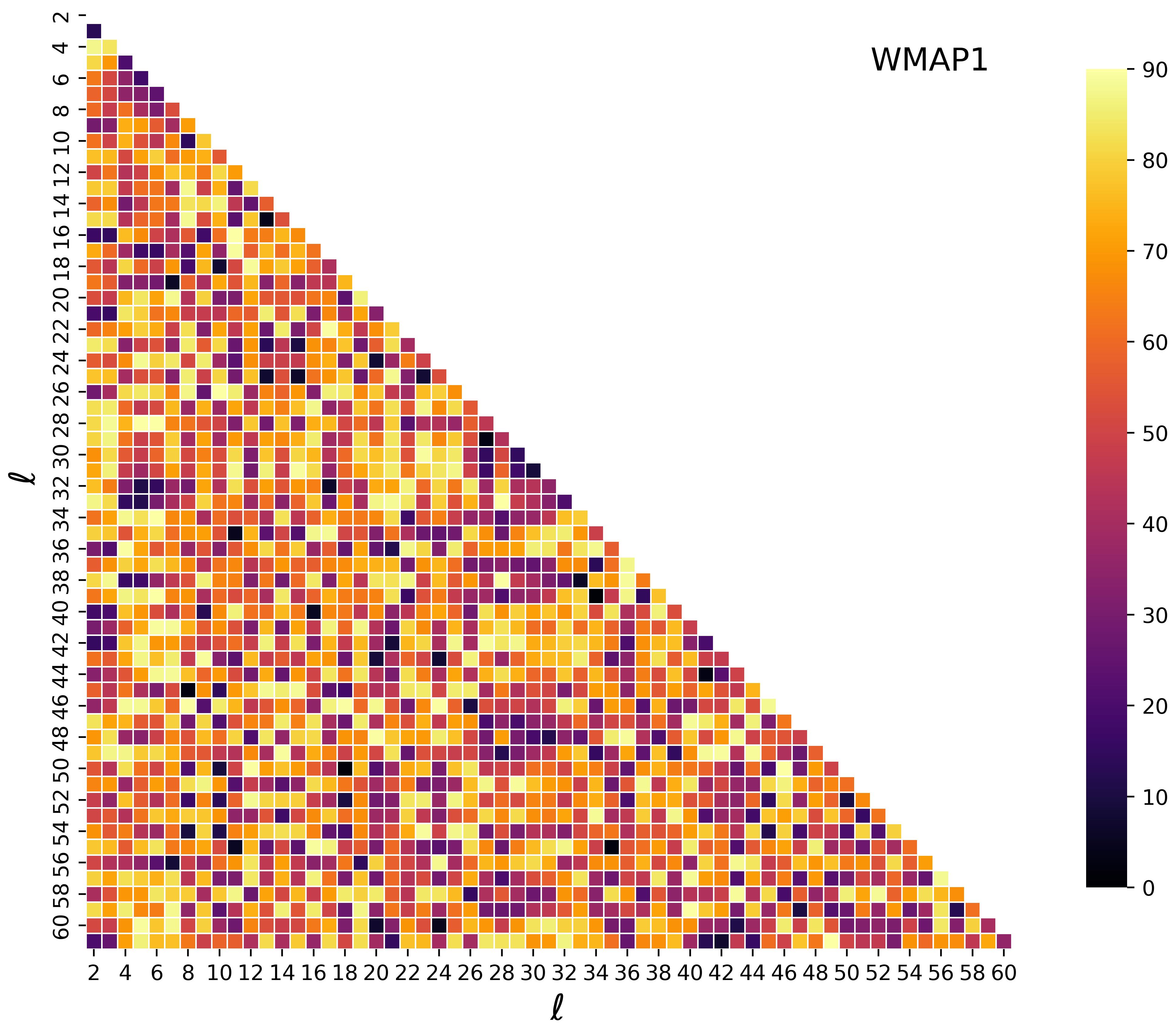
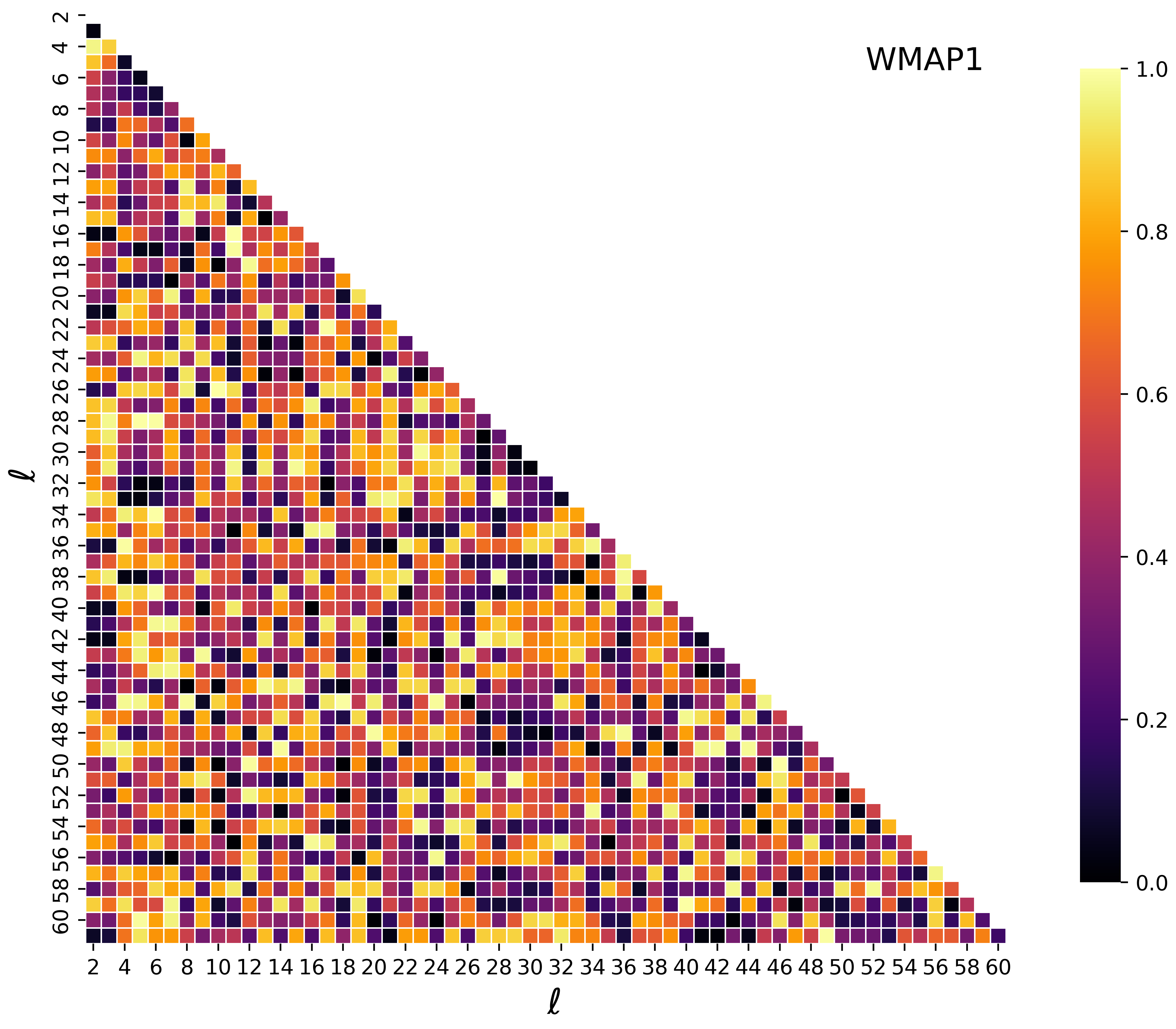
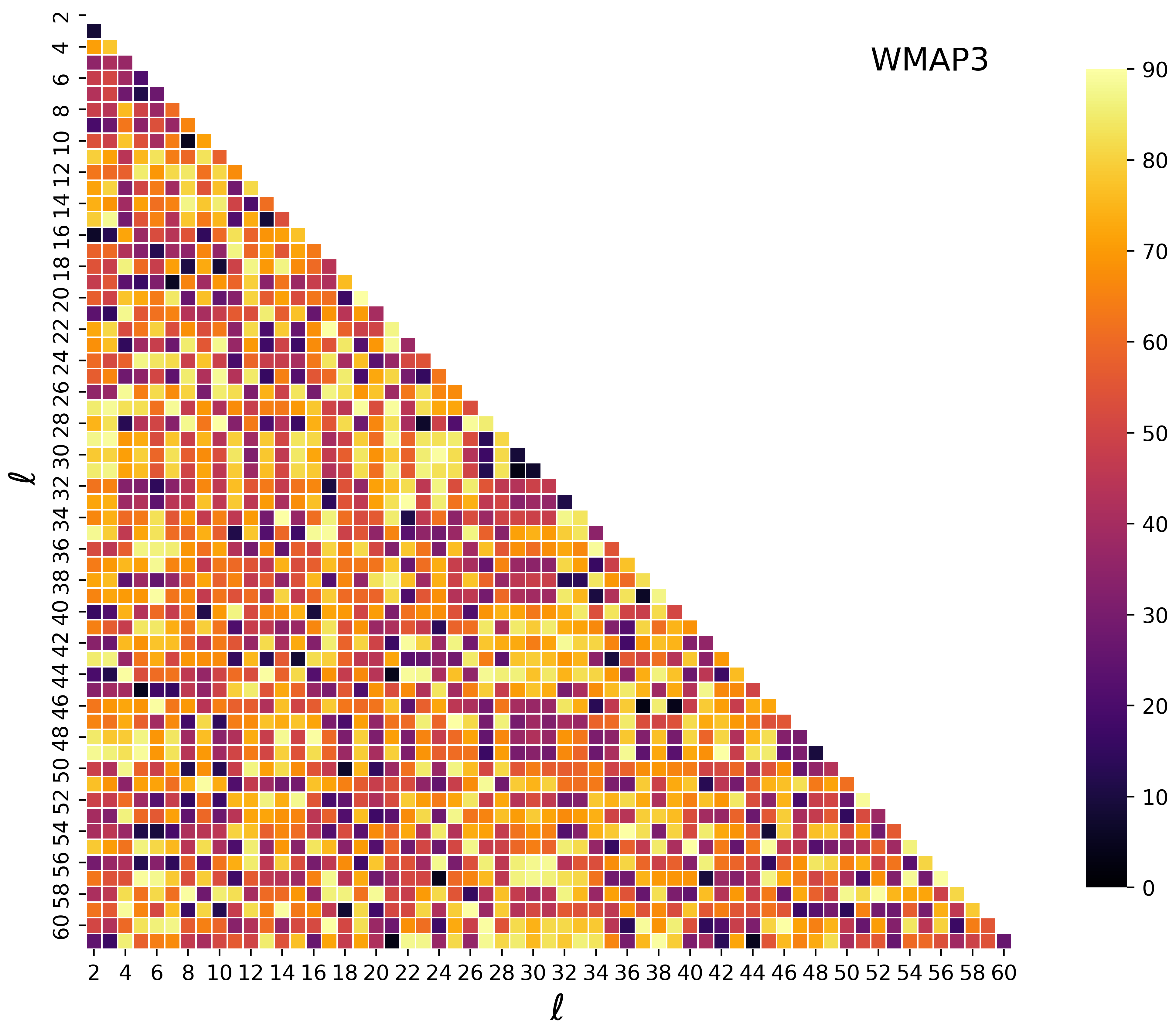
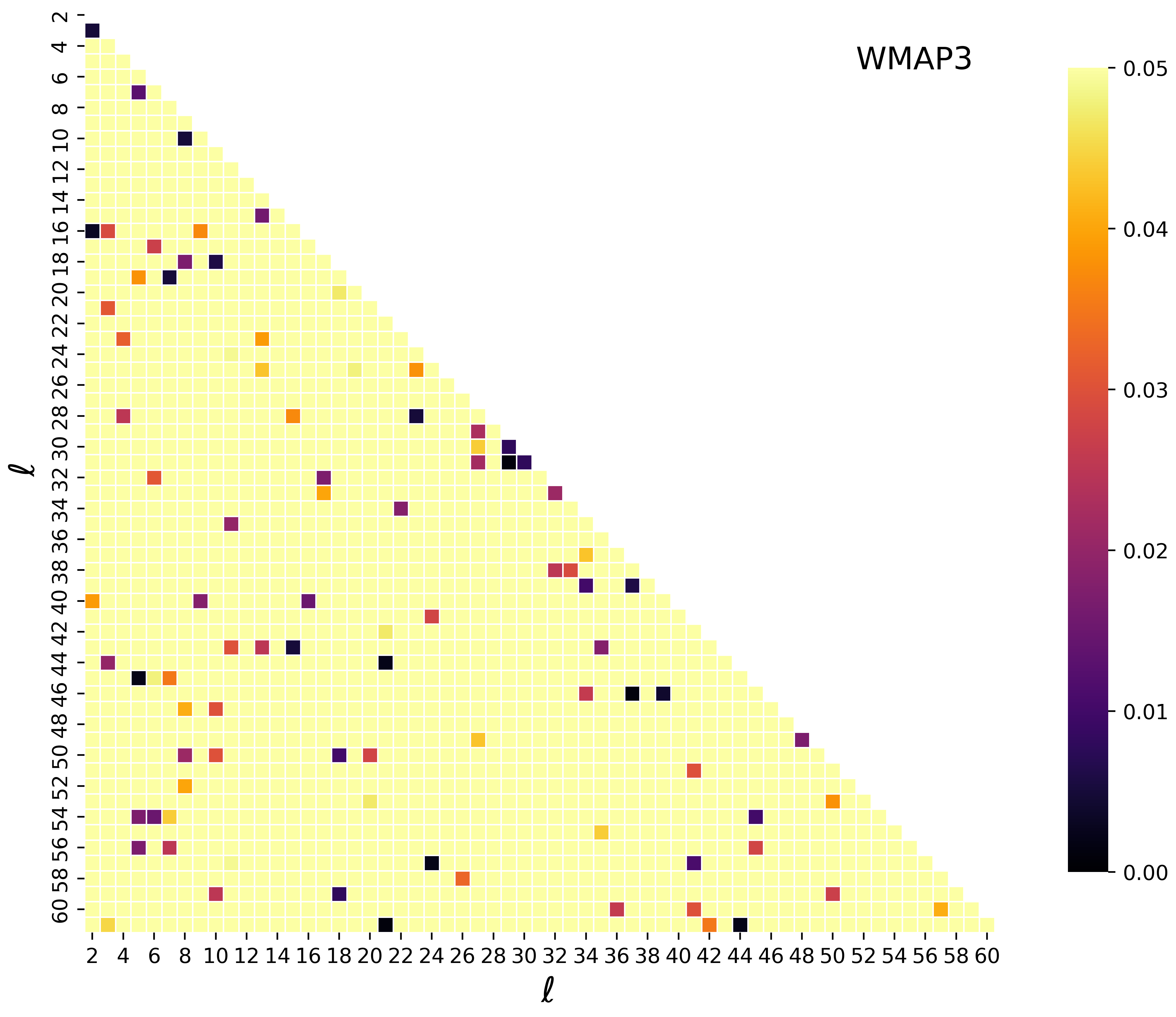
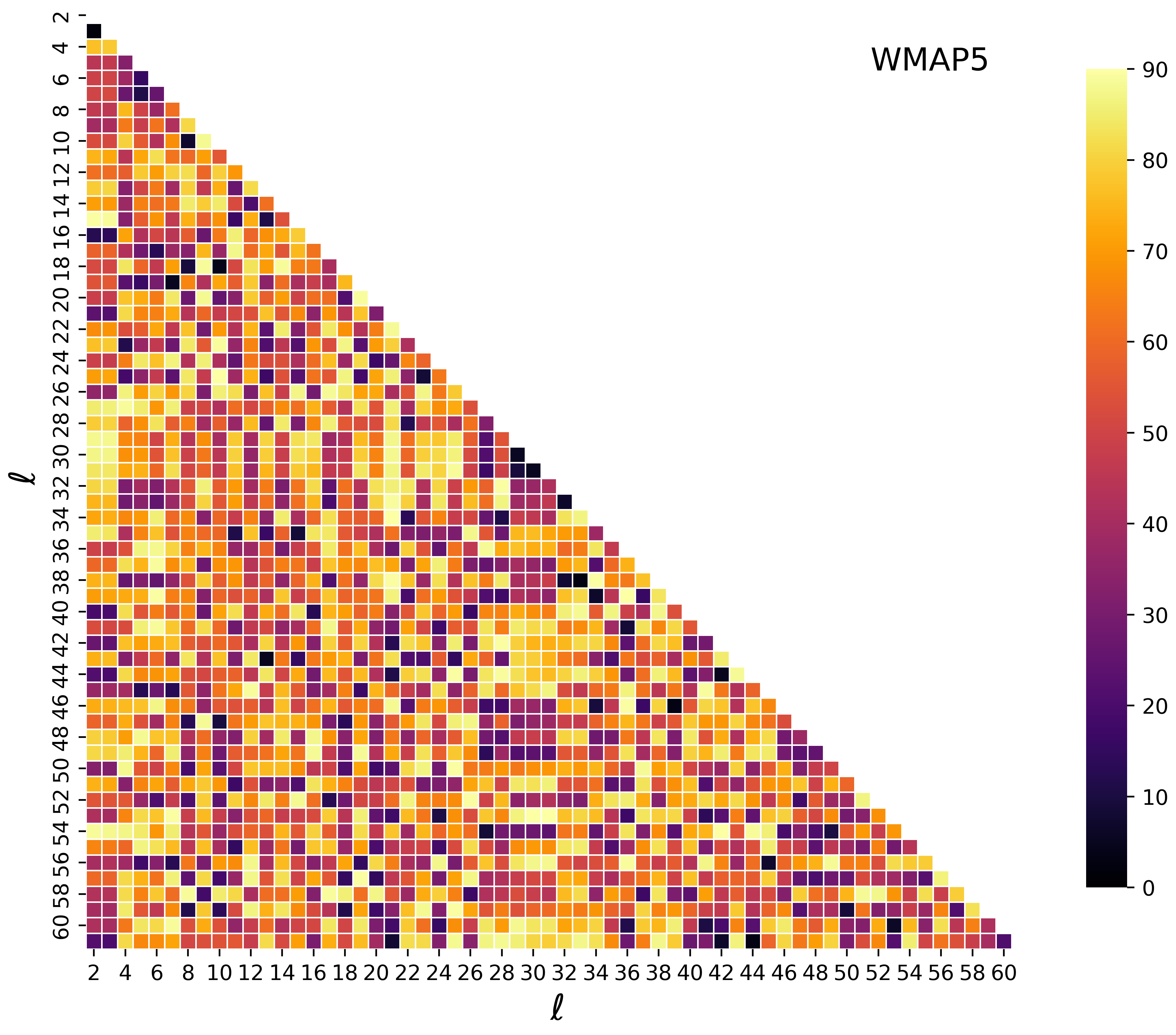
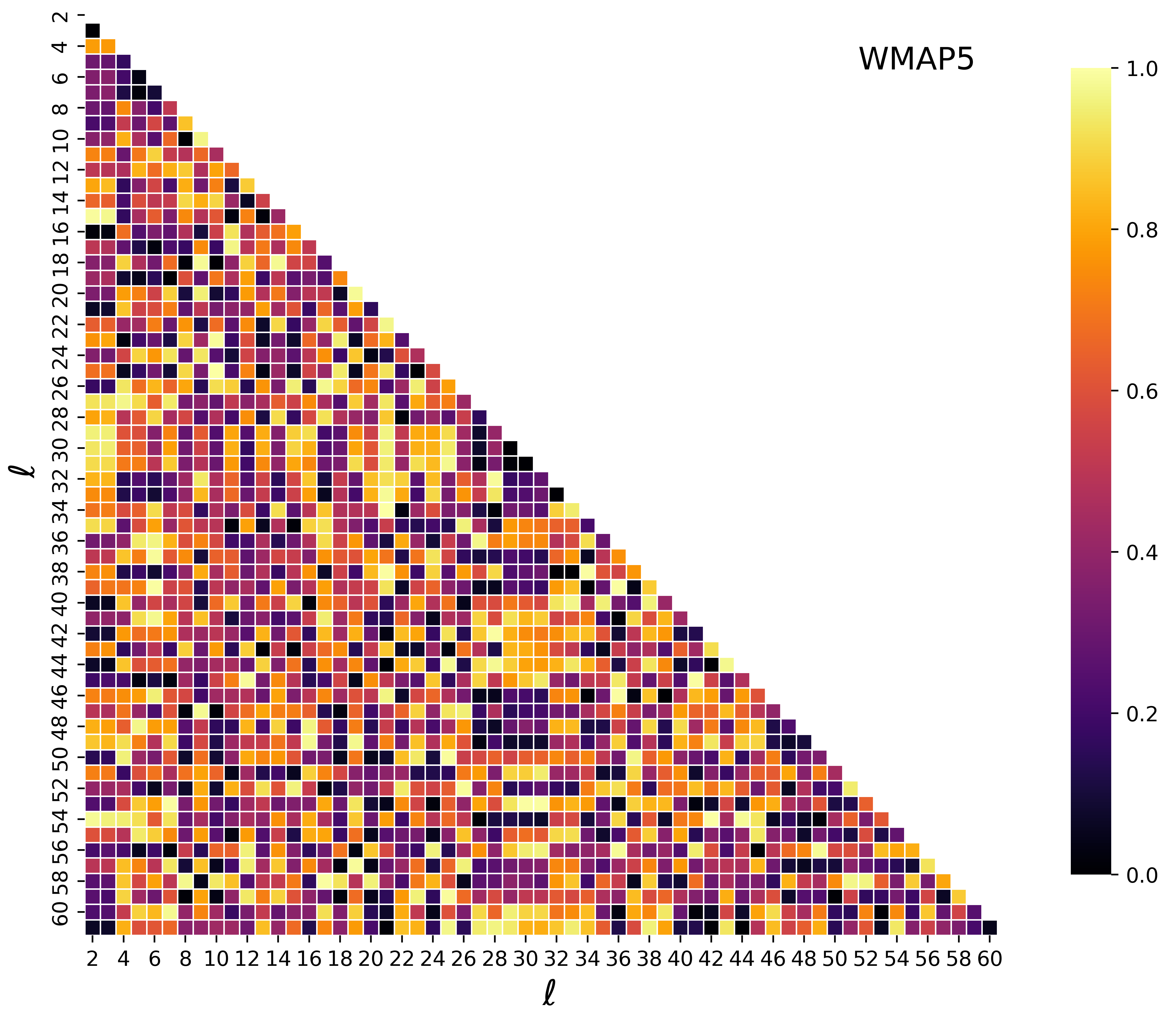
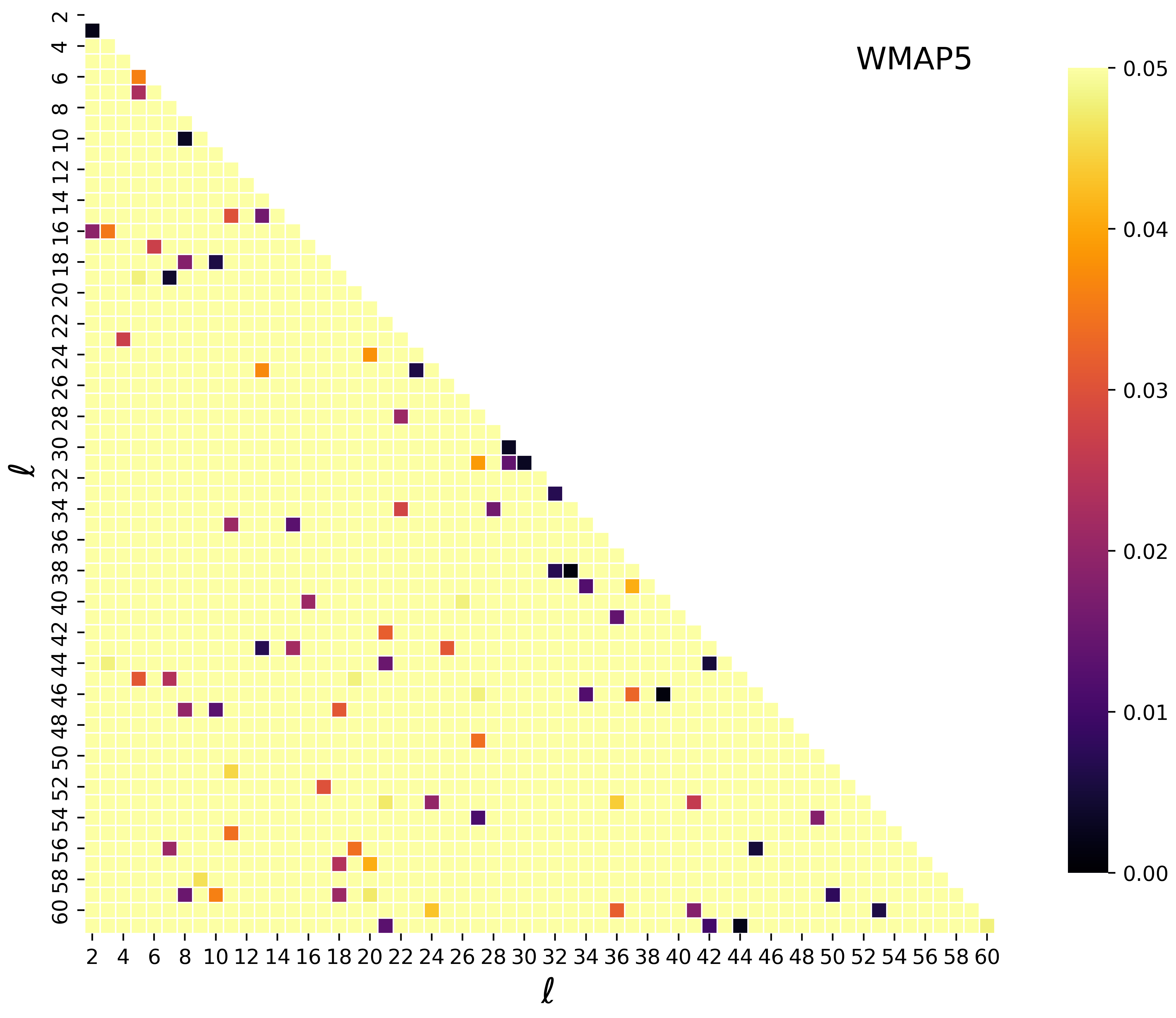
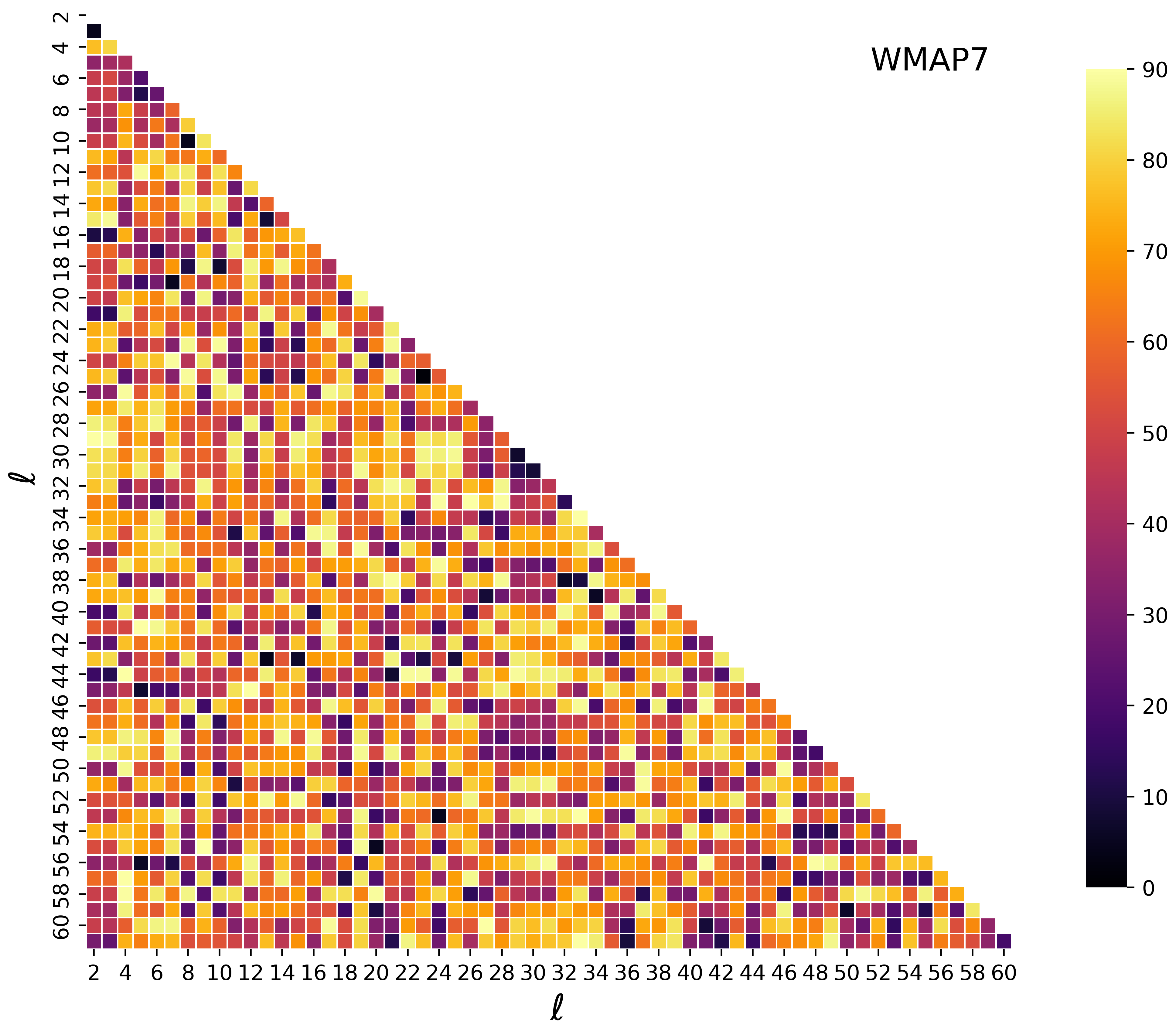
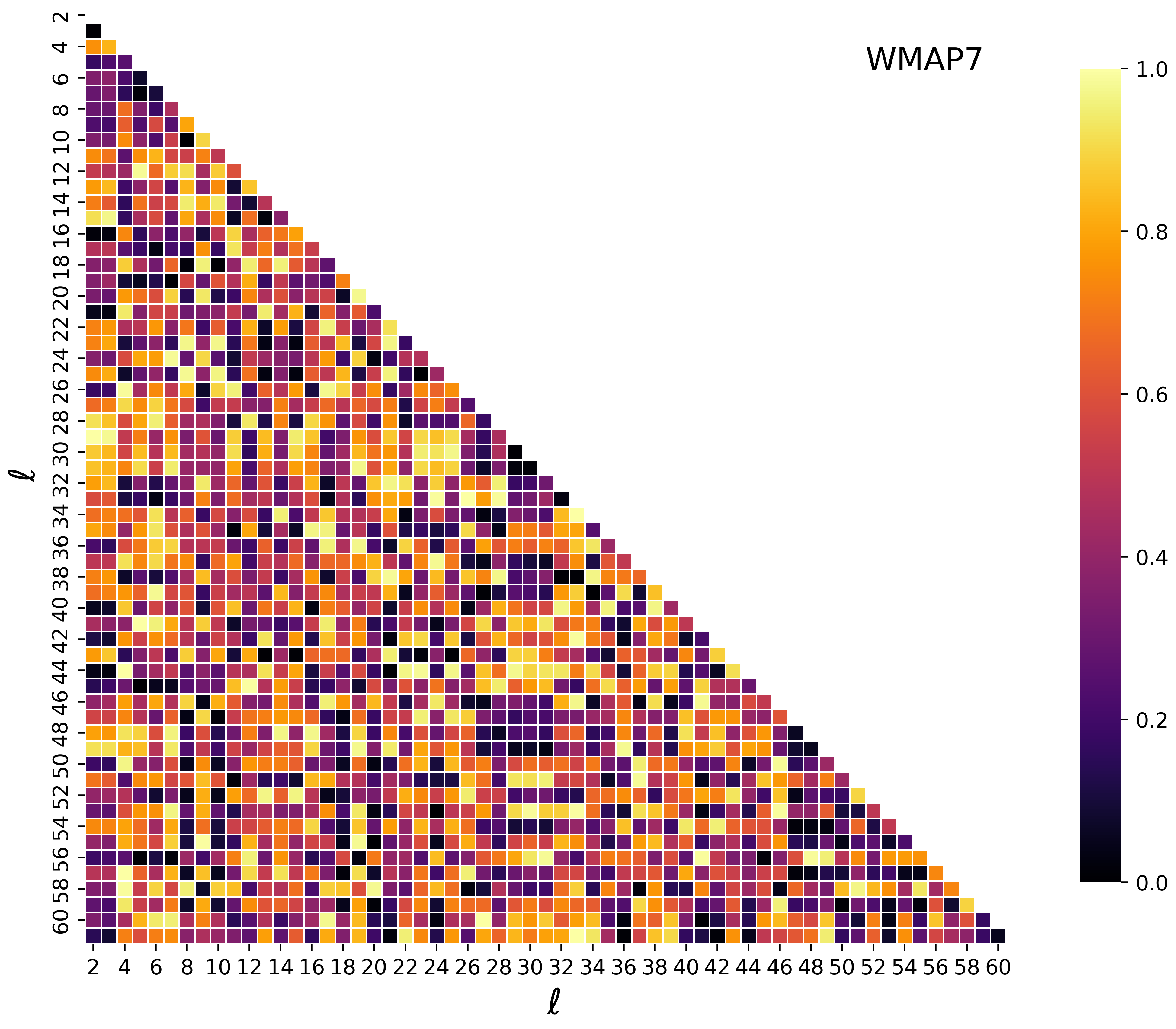
Figure 4: Left column depicts the alignment angle observed between any two multipoles in a cleaned CMB map, as a lower triangle plot whose colour denotes the angle of alignment. Middle column depicts the $p$-value plot, in the same manner, for the observed alignment angle as estimated from simualtions. The right column highlights those modes whose alignment angle is anomalous with a $p$-value of $p\leq 5\%$. Cleaned CMB maps for which the results are presented here are the ILC CMB maps from WMAP 1 (first row), 3 (second row), 5 (third row), and 7 (fourth row) years of data.

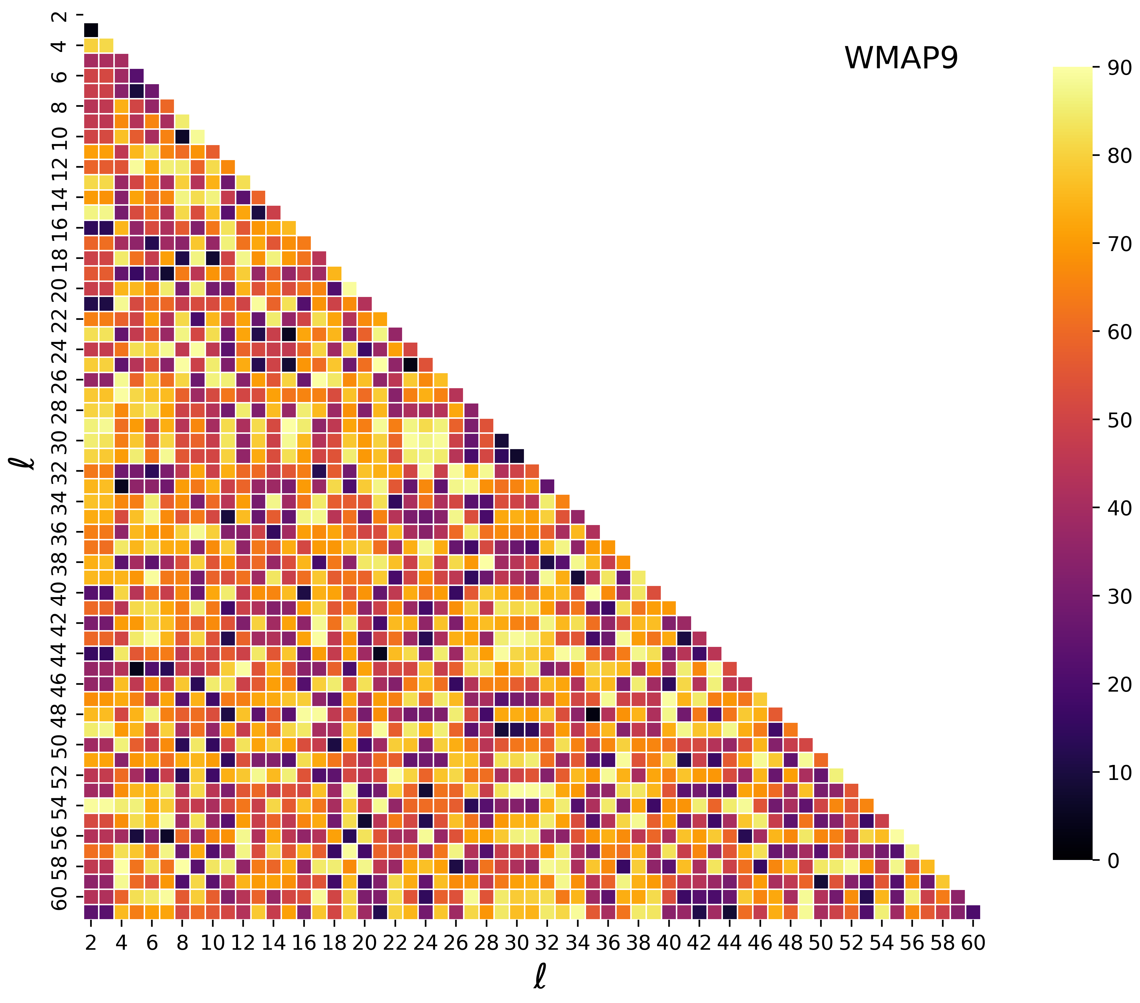
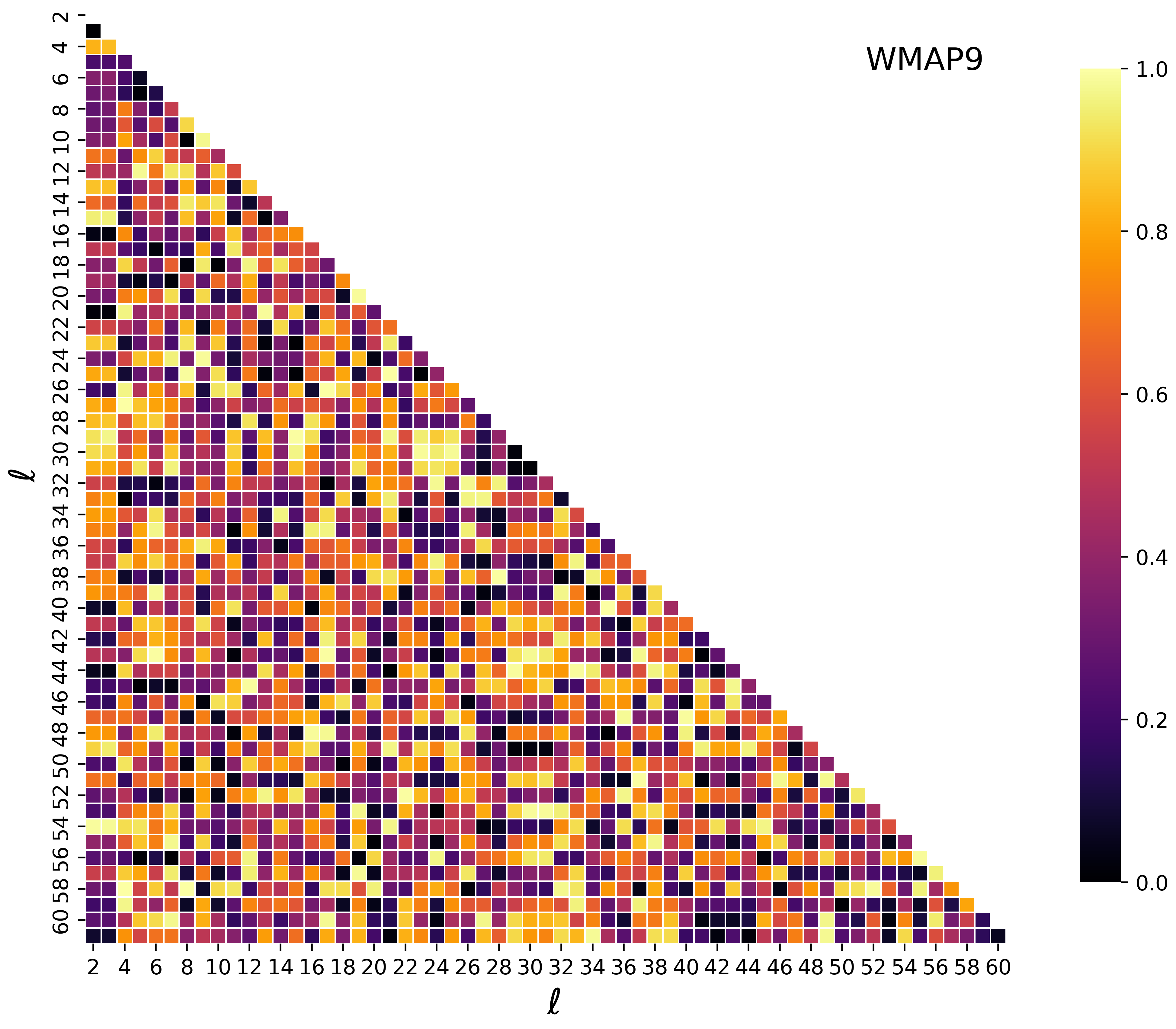
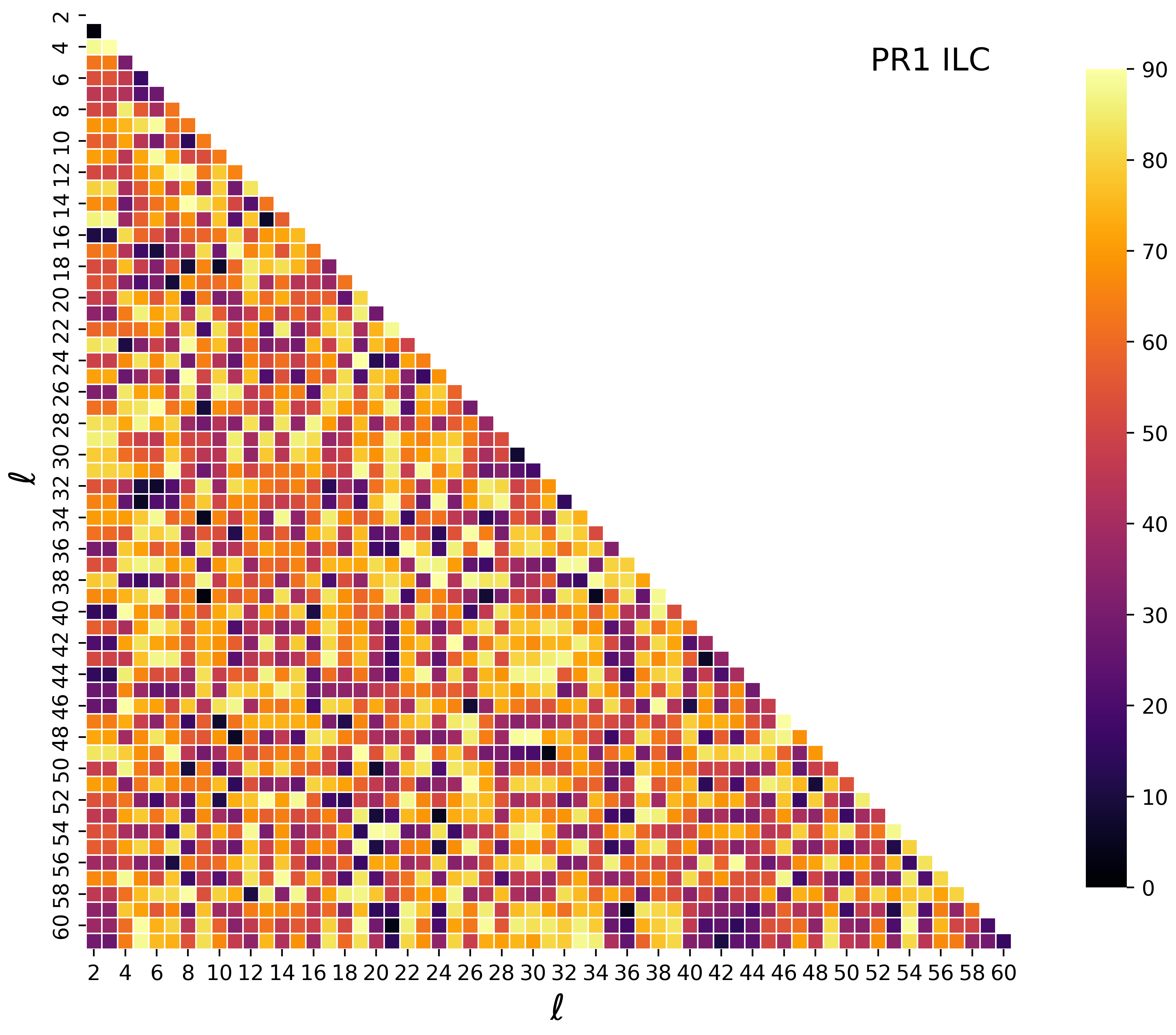
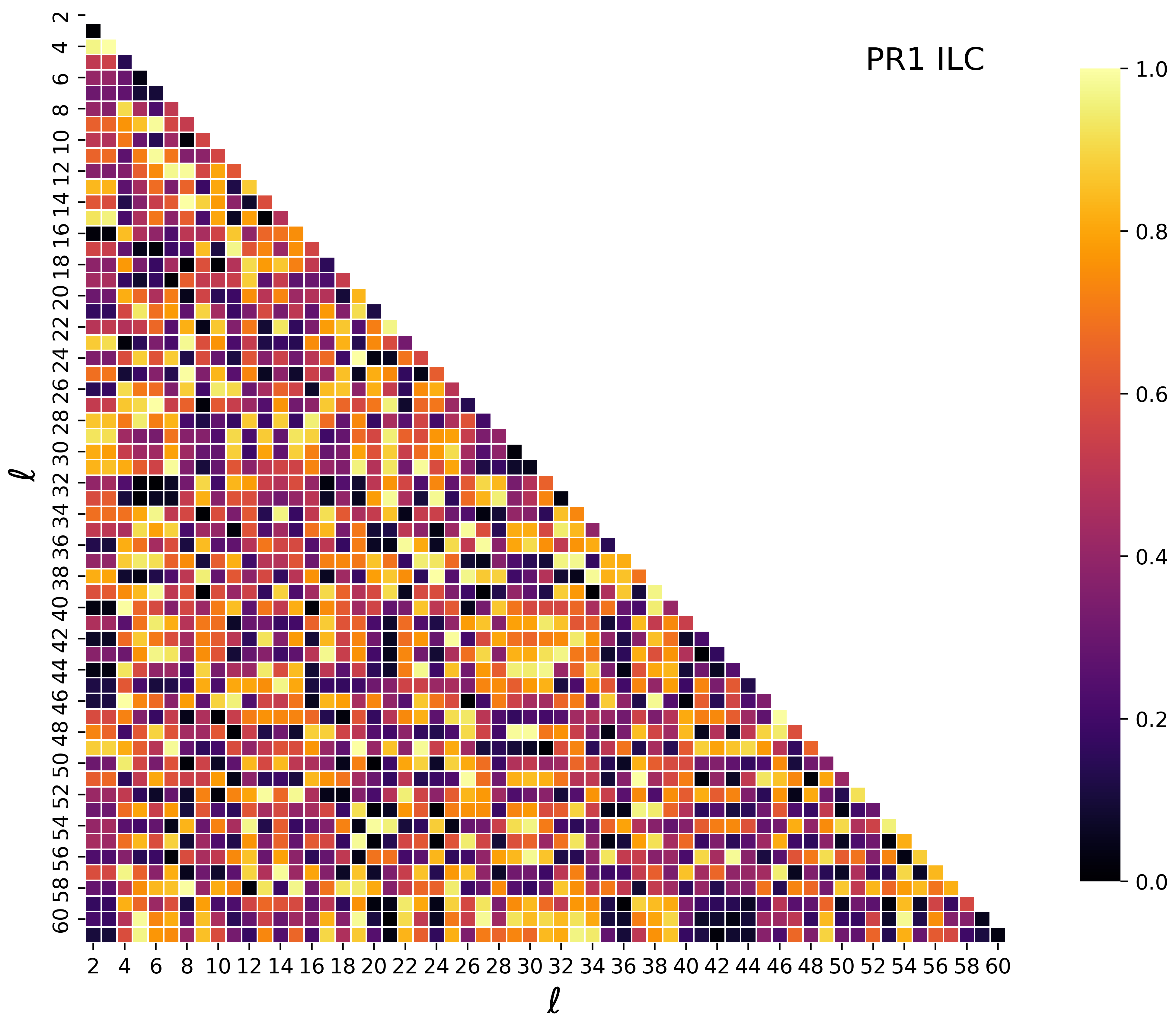
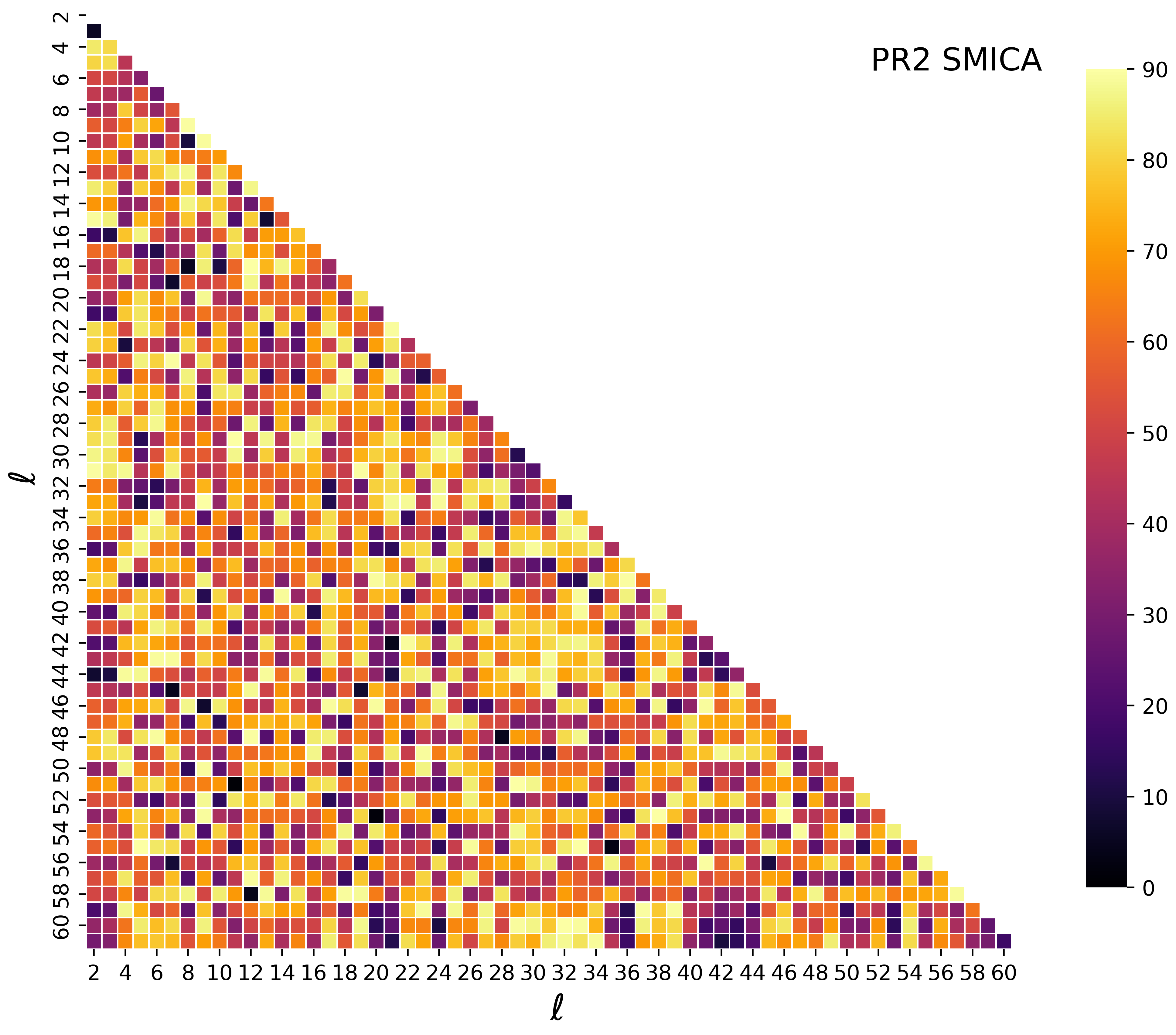
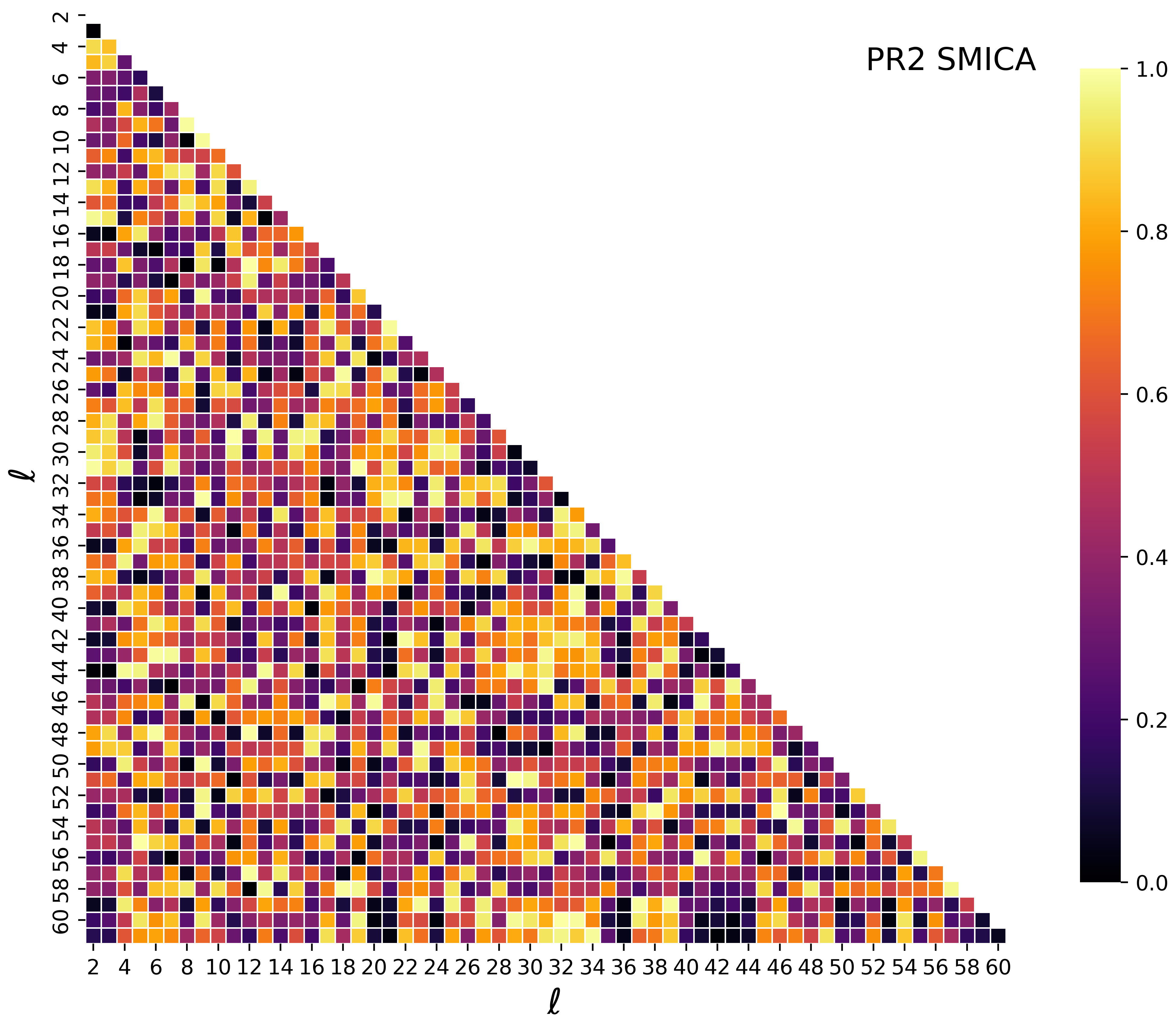
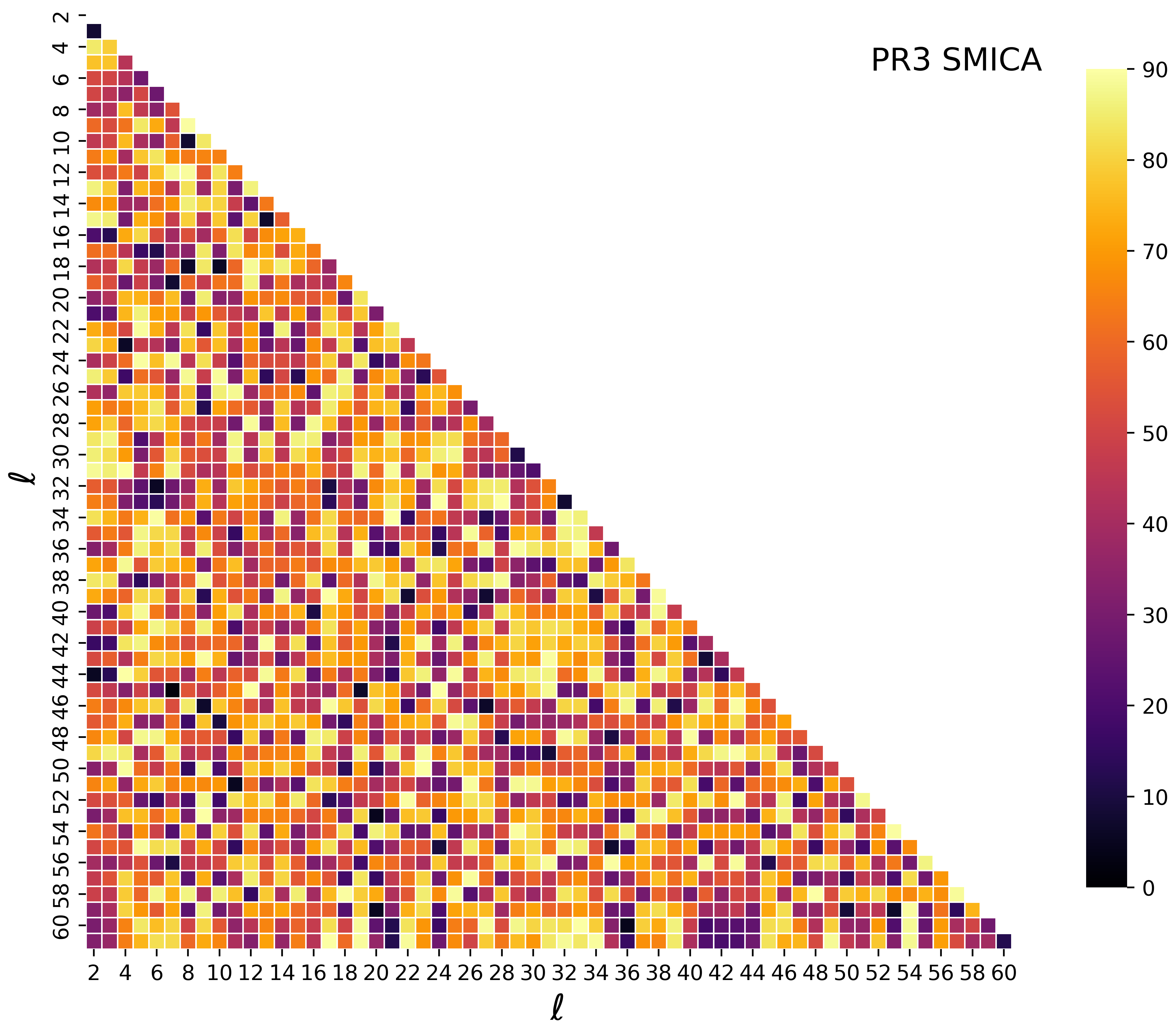
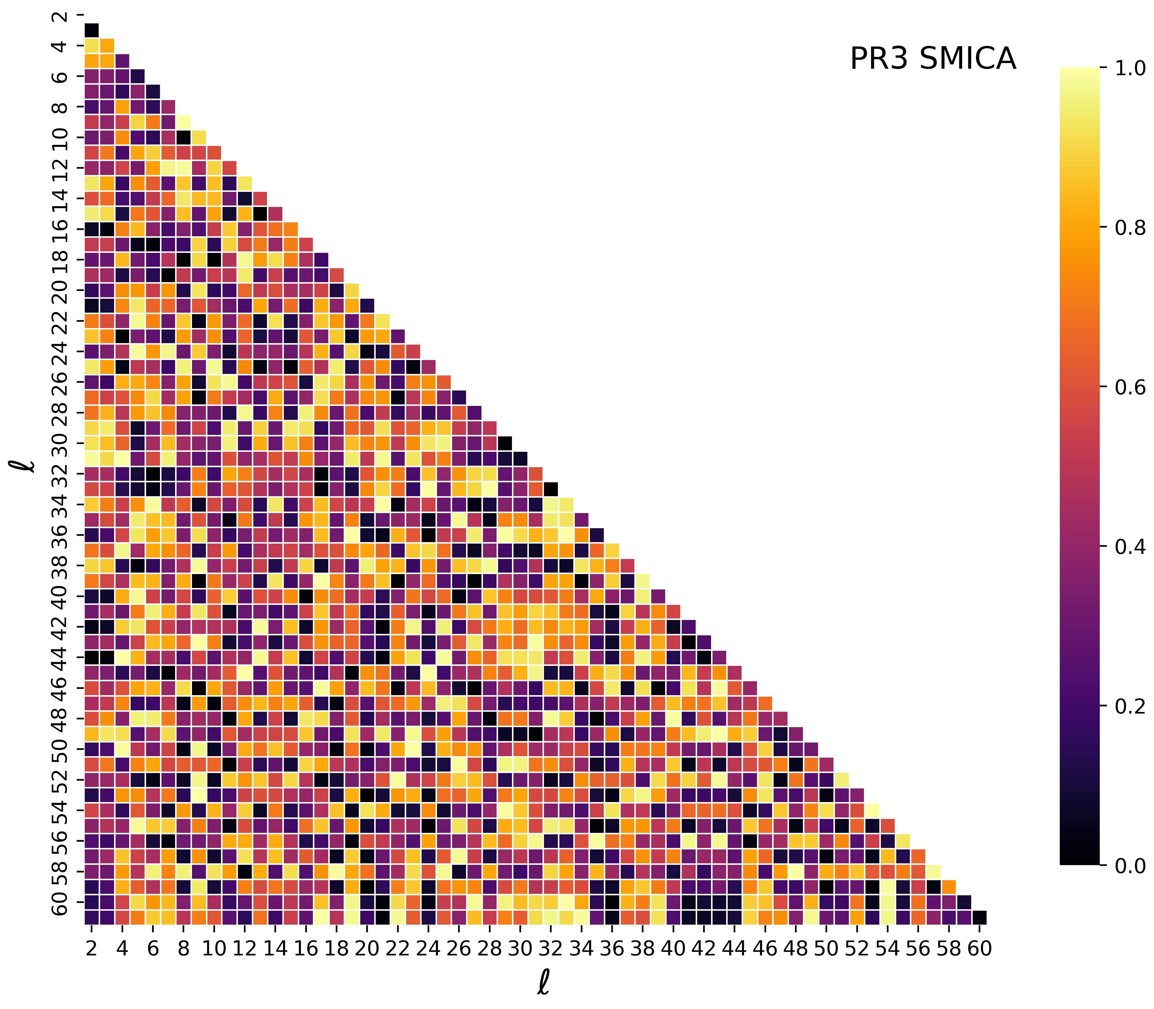
Figure 5: continued

Same as previous figure, but for ILC cleaned CMB map from WMAP 9 years of data (first row) as provided by WMAP team, ILC cleaned Planck 2013 PR1 data (second row) obtained by us, SMICA cleaned CMB maps from Planck 2015 data (third row) and 2018 data release (fourth row) as provided Planck teams respectively.

Number of multipole pairs with an anomalous alignment of $p\leq 0.05$, and the corresponding cumulative binomial probability of finding as many aligned modes or more as seen in data from each data release are given in Table 3. We find that the collective number of multipole pairs that are anomalously aligned is insignificant. Their pairwise alignments do not indicate any violation of isotropy. Also computed is the probability of observed Kuiper ($V$) statistic, as defined in Eq. (7), of alignment measures from each data CMB map considered in the present study. Recall that the alignment measure is defined as ‘$x=1-\tilde{\bf e}_{l}\cdot\tilde{\bf e}_{l^{\prime}}$’ where $\tilde{\bf e}_{l}$ and $\tilde{\bf e}_{l^{\prime}}$ are the PEVs corresponding to multipoles $l$ and $l^{\prime}$ respectively. Kuiper statistic is a CDF statistic, that is used here to check the conformity of the distribution of multipole PEV alignments with a uniform distribution ($x\in[0,1]$) as expected in the standard cosmological model. This statistic, as computed from data, is compared with the same statistic derived from simulations and the respective $p$-values thus found are given in column 4 of Table 3. Again we don’t find any deviation from the null hypothesis that the principal eigenvectors of various multipoles are randomly oriented with respect to each other.

Data set	$k_{*}$	Cumulative	$p$-value of $V$
	(out of 1770)	Probability
WILC 1yr	82	0.775	0.307
WILC 3yr	92	0.366	0.562
WILC 5yr	81	0.808	0.850
WILC 7yr	93	0.327	0.416
WILC 9yr	81	0.808	0.547
PR1 ILC	88	0.537	0.625
PR2 SMICA	89	0.494	0.904
PR3 SMICA	91	0.408	0.816

Table 3: For the cleaned CMB temperature anisotropy maps considered in the present study as listed in column 1, the number of anomalous alignments among various multipoles shown in Fig. [4] and Fig. [5] are listed in column 2. For the multipole range that we are interested in i.e., $l=[2,61]$, there are $n=60*59/2=1770$ possible combinations to consider, of which the number of anomalous alignments ($k_{*}$) defined as having a probability of $p\leq 0.05$ are mentioned in column 2. Column 3 lists the cumulative binomial probability of finding ‘$k_{*}$’ number of modes out of ‘$n$’ that were considered following Eq. (6). Taking these 1770 possible alignments among the first 60 low multipoles, the empirical CDF (eCDF) of these alignments defined as $x\equiv 1-\cos\alpha_{ll^{\prime}}=1-\hat{e}_{l}\cdot\hat{e}_{l^{\prime}}$ is compared with eCDF from simualtions using Kuiper ($V$) statistic. The probability to exceed the observed value of $V$-statistic from the data is given for each map we analyzed in column 4, using appropriately generated simulations.

4.4 Collective alignments of low multipoles

Finally, we test for the presence of any collective alignments among the first sixty low multipoles of CMB sky as estimated from WMAP’s five data releases using ILC method, Planck public release 1 data that is also processed using ILC method (by us), and the SMICA cleaned CMB maps from Planck’s 2015 and 2018 data releases.

For this, we employ the Alignment tensor (AT) as defined in Eq. (8). For each of the CMB maps that we studied in this work, Alignment tensor is computed using the PEVs of first sixy multipoles i.e., $l=2$ to $61$ and the corresponding Alignment entropy (AE) is computed. These AE from data, $S_{X}^{\rm obs}$, are compared with AE obtained from corresponding simulation ensembles, $\{S_{X}^{\rm sim}\}$, to evaluate the significance of observed AE in the data. Accordingly, the eigenvector corresponding to the largest eigenvalue of AT will assume significance as representing a preferred collective alignment axis for the set of multipoles being studied.

In the top panel of Fig. [6], we present the significances of observed $S_{X}$ from various data releases of CMB sky thence derived. One readily notices that the $p$-values of $S_{X}^{\rm obs}$ from any of the full-sky cleaned CMB maps are not significant. Thus, there is no particular preference in the alignments among the PEVs of the first sixty multipoles in any of the CMB maps considered.

In the bottom panel of Fig. [6], we have shown the collective alignment axes of the first sixty multipoles, as represented by the eigenvector corresponding to the largest eigenvalue of AT i.e., $\tilde{\bf f}$, for all the CMB maps from various data releases as indicated in the figure. Since the observed $S_{X}$ in these maps are not significant, these axes doesn’t assume any importance. Nevertheless, they are depicted here for completeness.

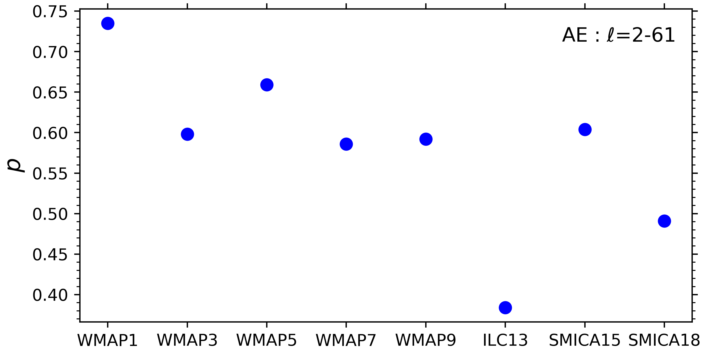
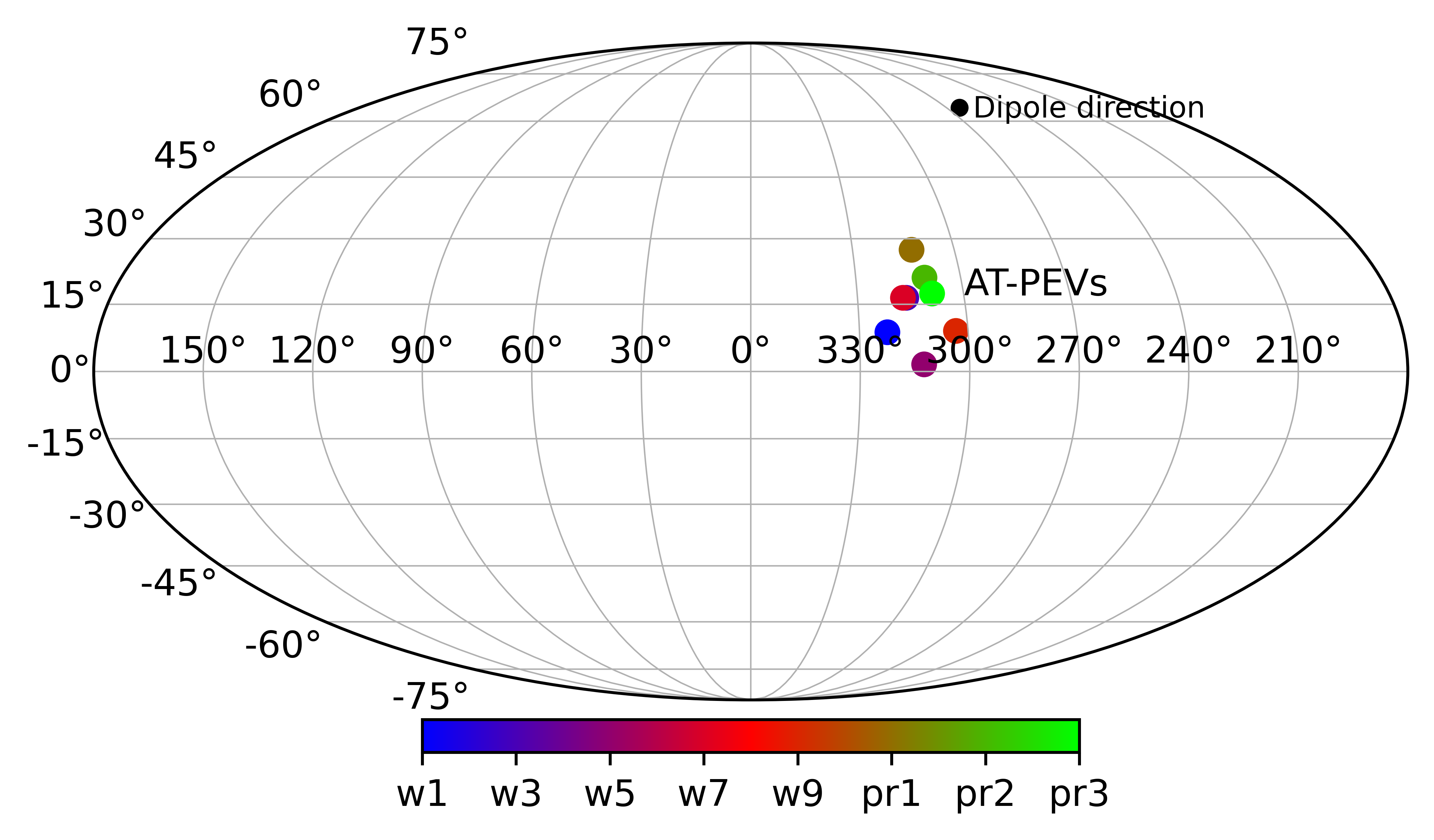
Figure 6: Top : $p$-values of Alignment entropy as seen in CMB maps for various data releases mentioned on x-axis. Bottom : Collective alignment axes of multipoles $l=[2,61]$ i.e., the first sixty multipoles from all data releases of WMAP and Planck as indicated. w1, w3, etc., refer to WMAP 1yr, 3yr , etc., and pr1, etc., are Planck public release 1, etc.

4.5 Common set of anomalous multipoles across CMB data

Abridging our findings so far, in this section, we present the list of multipoles and multipole combinations whose random chance occurance probability when employing a particular statistic was found to be $\leq 5\%$. The results presented are for the instances of anomalous Power entropy, anomalous alignments of higher multipoles with the quadrupole ($l=2$), and any pair of anomalous modes which are found to be spuriously aligned across all CMB maps (ie., data sets) considered in this work. These are summarized in Table [4].

Statistic	Multipole(s), $l$
Power Entropy	13, 30
Aligned with Quadrupole	3
Aligned modes	(2, 3), (3, 16), (6, 17), (7, 19), (7, 56),
	(8, 10), (10, 18), (11, 35), (13, 15),
	(16, 40), (21, 61), (22, 34), (23, 25),
	(29, 30), (34, 39)

Table 4: Common set of anomalous multipoles across data sets corresponding to each statistic listed in column 1 are consolidated here, whose $p$-values for a particular statistic were found to be $p\leq 0.05$.

5 Conclusions

In this paper, we analyzed all full-sky CMB maps that are publicly available from NASA’s WMAP’s 1, 3, 5, 7 and 9 years of observational data as well as CMB maps from ESA’s Planck’s 2013, 2015 and 2018 public releases. Particularly, we studied CMB maps obtained using internal linear combination (ILC) method from WMAP’s successive data releases and Planck’s PR1 data, and the SMICA cleaned CMB maps from Planck’s full (PR2) and legacy (PR3) data releases. Thus a total of eight full-sky cleaned CMB maps released from WMAP and Planck satellite teams between 2003 and 2018 were analyzed in our present study.

Our objective was to probe alignments among the first sixty large angular scale modes of the CMB sky i.e., $l=2$ to $61$. To do so, we employed the Power tensor (PT) method that maps the intricate pattern of an observed CMB mode to an ellipsoid whose orthogonal axes define an invariant frame for that CMB mode and the axes lenghts’ given by the eigenvalues of the Power tensor represent deviation from isotropy. If a multipole is statistically isotropic, the corresponding PT’s (normalized) eigenvalues i.e., the axes lengths are equal to $1/3$. These eigenvalues can then be combined in an invariant way using the Power entropy ($S$) statistic, whose maximum is $\ln(3)$ implying perfect isotropy and whose minimum being ‘$0$’ denotes maximal aniostropy. Independent of PT’s eigenvalues, eigenvector corresponding to the largest eigenvalue of PT of a multipole can be taken to represent an axis of anisotropy for that CMB mode called principal eigenvector (PEV). These PEVs can be compared with each other to probe any preferred alignments among them. In case of maximal anisotropy ($S\rightarrow 0$) for some multipole, its PEV truly represents an axis of anisotropy for that mode.

We found that the mutlipoles $l=13,30$ have anomalous power entropy (deemed to be so by having a random chance occurrence probability of $\leq 0.05$) in all the CMB maps analysed. Thus these are truly anisotropic modes that are robust with respect to accumulated data, evolving analysis procedures applied to data, and between two different CMB missions with different systematics. Their axis of anisotropy are shown in the top panel of Fig. [7] from various data sets studied. Their mode patterns are shown in the bottom two panels i.e., for $l=13$ and 30 respectively in the same figure. Cumulatively also, we find that, the number of intrinsically anisotropic modes in a CMB map from a particular data release is not significant.

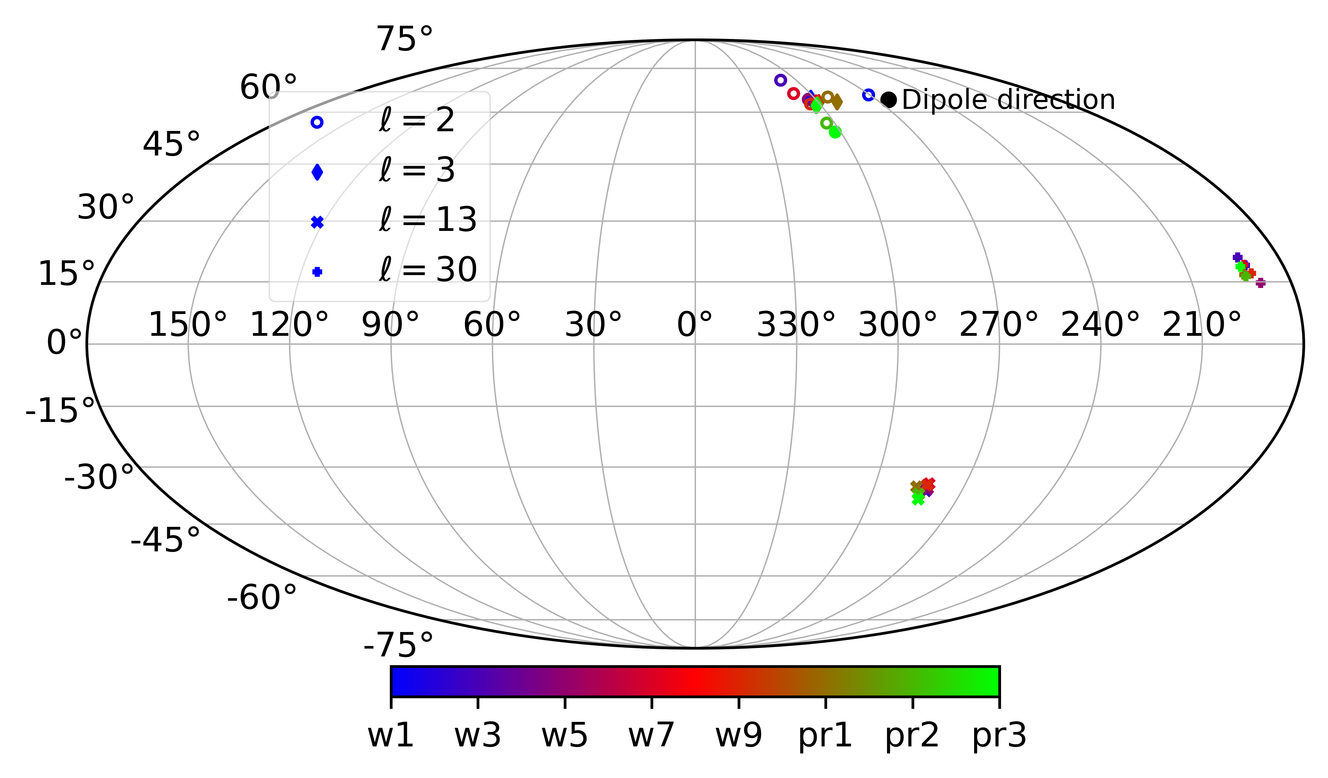
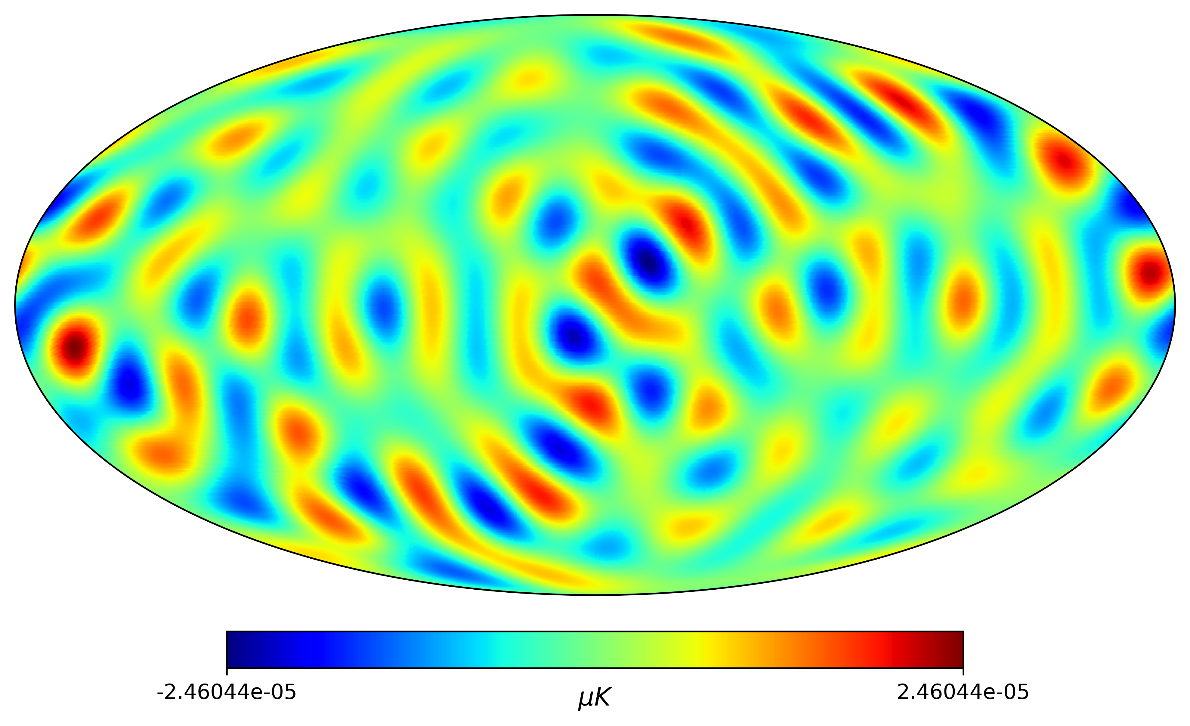
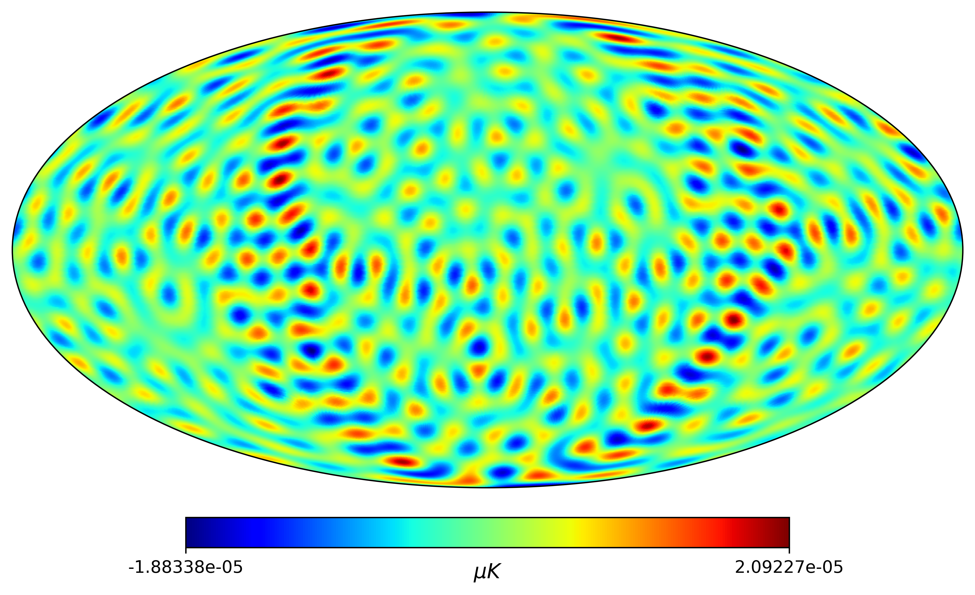
Figure 7: Top : The anisotropy axis of consistently aligned modes $l=2,3$ are shown here, along with the PEV axes of multipoles having anomalous Power entropy consistently in all data sets viz., $=13,30$ that we studied in the present work. Middle and Bottom : Multipole patterns of anomalous Power entropy modes $l=13,30$ are shown here from Planck’s 2018 SMICA CMB map whose random chance occurrence probability is $p\leq 5\%$.

Then, we examined any preferred alignments of higher multipoles with the quadrupole ($l=2$) in each of these full-sky cleaned CMB maps. Only the quadupole and octopole were found to be consistently well aligned in all the CMB maps from various data sets. Again this indicates the robust nature of their alignment that is independent of analysis procedures used and systematics. So the spurious alignment between the two largest cosmologically significant multipoles in CMB maps derived from WMAP’s first year data release, remains to be so in the CMB maps from final public data release (PR3) from PlanckṪhe anisotropy axes (PEVs) of $l=2,3$ modes from CMB maps across all data sets we analysed are also shown in top panel of Fig. [7] with different point types.

In the standard model, where different multipoles are expected to be uncorrelated, PEVs will be oriented randomly with respect to each other. So an alignment measure defined as ‘$x=1-\cos\alpha_{ll^{\prime}}$’ where $\alpha_{ll^{\prime}}$ being the angular separation between the quadrupole ($l=2$) and rest of the higher multipoles ($l^{\prime}=3$ to $61$) are expected to follow a uniform distribution in the range $x=0$ to 1. Then using a cumulative distribution function (CDF) statistic, specifically, Kuiper’s $V$ statistic, we studied the alignment measures’ agreement with a uniform distribution in the range $x\in[0,1]$. We infer that the Kuiper’s statistic doesn’t indicate any preferred alignment of higher multipoles with the quadrupole.

Going beyond alignment preferences of other multipoles with $l=2$, we also probed for the presence of any unexpected alignments between pairs of multipoles $l,l^{\prime}\in[2,61]$. Again we find that the number of such aligned multipole pairs with a $p$-value $\leq 5\%$ is insignificant. Their cumulative probability, and the CDF analysis of their alignment measures also doesn’t indicate any deviation from isotropy.

Finally, we probed collective alignments among the first sixty multipoles viz., $l=2$ to 61. To that end, we employed the Alignment tensor, X. Alignment tensor is formed by using the PEVs corresponding to the range of multipoles of our interest. Its eigenvalues are combined to form Alignment entropy, $S_{X}$, which informs us of any preferred orientation among the PEVs used. We find that $S_{X}^{\rm obs}$ is insignificant for all the eight CMB maps that we studied in the present work. $p$-values of observed Alignment entropy derived from corresponding simulation ensembles are consistent with standard model expectations. Hence we conclude that, collectively, there is no preferred alignment among the low multipoles $l=[2,61]$.

Appendix A Data and simulations

A.1 Data

Wilkinson Micrwave Anisotropy Probe (WMAP) is a space based NASA mission which made observations of the microwave sky in five frequency channels 23, 33, 41, 61 and 94 GHz. These five frequency channels are also referred to as $K,Ka,Q,V,$ and $W$ bands respectively. Cleaned CMB maps from these five raw satellite data were obtained using the internal linear combination (ILC) method where suitable weights were used to remove foregrounds. The observed signal in a frequency channel, $\nu_{i}$ (or simply $i$), is supposed to be a linear combination given by,

$$\Delta T_{i}(\hat{n})=\Delta T_{c}(\hat{n})+F_{i}(\hat{n})+N_{i}(\hat{n})\,,$$ (10)

where $\Delta T_{c}(\hat{n})$ is the cosmic CMB signal independent of frequency (in thermodynamic units), $F_{i}(\hat{n})$ represents sum of all foregrounds (galactic/extra-galactic astrophysical emission) at frequency ‘$i$’ that are frequency dependent, and $N_{i}(\hat{n})$ is the detector noise in channel ‘$i$’. When the observed sky is digitized using HEALPix the sky positions, $\hat{n}$, are equivalently described by pixel indices ‘$p$’ whose pixel centers represent the direction of arriving photons that are reaching us.

Taking linear combination of raw maps from different frequencies, we get an estimate of the CMB sky to be,

$$\Delta\hat{T}_{c}(p)=\sum_{i=1}^{n_{c}}w_{i}\Delta T_{i}(p)=\Delta T_{c}(p)\sum_{i=1}^{n_{c}}w_{i}+\Delta T_{\rm res}(p)$$ (11)

where $\Delta T_{\rm res}(p)=\sum_{i=1}^{n_{c}}w_{i}[F_{i}(p)+N_{i}(p)]$ and $n_{c}$ are the total number of frequency channels. Thus the ILC weights are obtained by minimizing the variance of the cleaned map, $\Delta\hat{T}_{c}(\hat{n})$, subject to the constraint that $\sum_{i}w_{i}=1$ so that the cosmic CMB signal remains untouched while residual term in minimum or effectively zero. The variance of cleaned CMB map is given by

$$\sigma^{2}_{c}=\langle\Delta\hat{T}_{c}^{2}(p)\rangle-\langle\Delta\hat{T}_{c}(p)\rangle^{2}={\bf w}^{T}{\bf C}{\bf w}\,,$$ (12)

where ${\bf w}=(w_{1},w_{2},\ldots,w_{n_{c}})^{T}$ is the $n_{c}\times 1$ column vector of weights, $\langle...\rangle$ represents expectation value of a quantity inside the angular brackets, and

$$C_{ij}=[{\bf C}]_{ij}=\frac{1}{N_{pix}}\sum_{p=1}^{N_{pix}}(\Delta T_{i}(p)-\overline{\Delta T}_{i})(\Delta T_{j}(p)-\overline{\Delta T}_{j})\,,$$ (13)

is the covariance matrix between different frequency maps and $\overline{\Delta T}_{i}$ is the average of all pixels of frequency map ‘$i$’.

Since the foreground strength varies across the sky, the ILC procedure is applied by dividing the observed sky into different regions as shown in Fig. [8]. In WMAP’s 1yr data release, a cleaned CMB map using ILC procedure is obtained by a non-linear minimization procedure (Bennett et al., 2003b). However Eriksen et al. (2004) showed that the ILC weights can be obtained analytically using the Lagrange multplier method as

$$\hat{{\bf w}}=\frac{{\bf C}^{-1}{\bf e}}{{\bf e}^{T}{\bf C}^{-1}{\bf e}}\,,$$ (14)

where ${\bf e}=(1,1,\ldots,1)^{T}$ is a $n_{c}\times 1$ column vector, and ${\bf\hat{w}}$ are the estimated weights for taking linear combination of raw satellite maps. Cleaned CMB maps thus obtained using the ILC procedure as provided by the WMAP team were used in the present study.

To employ real/pixel-space ILC method, all the input raw maps should have the same beam and pixel resolution. So the raw maps having different beam and pixel resolution were repixelized so that they have a common beam resolution given by a Gaussian beam of $FWHM=1^{\circ}$ at $N_{side}=512$ following,

$$a_{lm}^{\rm out}=\frac{b_{l}^{\rm out}p_{l}^{\rm out}}{b_{l}^{\rm in}p_{l}^{\rm in}}a_{lm}^{\rm in}\,,$$ (15)

in harmonic space, where $b_{l}$ is the circularized beam transfer function and $p_{l}$ being the pixel window function corresponding to the $N_{side}$ of a HEALPix digitized map. Here $b_{l}^{\rm in}=b_{l}^{i}$ where $i=K,Ka,Q,V,W$ bands of WMAP and $b_{l}^{\rm out}=b_{l}^{1^{\circ}}$ i.e., a one degree FWHM Gaussian beam transfer function. These $a_{lm}^{\rm out}$ are then converted into a map using HEALPix.

We also made use of ESA’s Planck satellite data as provided by Planck collaboration through their 2015 and 2018 data releases (for which complementary simulations are available). Particularly, we made use of the SMICA cleaned CMB maps in this work. They are available at a much higher resolution of HEALPix  $N_{side}$=2048. So, these are processed to get SMICA CMB maps at  $N_{side}$=512 smoothed to have a Gaussian beam $FWHM=1^{\circ}$, just like WMAP’s ILC CMB maps following Eq. (15). We note that SMICA foreground cleaning procedure is also an internal linear combination method, but performed in harmonic space using $a_{lm}^{i}$ i.e., spherical harmonic coefficients of raw satellite maps from different frequencies in which Planck made microwave sky observations viz., 30, 44, 70, 100, 143, 217, 353, 545, 857 GHz. The weights are computed using the formula,

$$\hat{{\bf w}}(l)=\frac{{\bf C}^{-1}_{l}{\bf e}}{{\bf e}^{T}{\bf C}^{-1}_{l}{\bf e}}\,,$$ (16)

similar to Eq. (14), where $C_{ij}(l)=\sum_{m=-l}^{l}a_{lm}^{i}a^{j*}_{lm}$. Specifically, weights for the SMICA procedure are obtained by fitting each element of the cross frequency channel covariance matrix $C_{ij}(l)$ as function of ‘$l$’ using a minimization procedure. For more details, the reader may consult Cardoso et al. (2008).

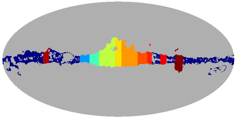
Figure 8: WMAP 9yr region masks (a total of 11) that were used to obtain the composite ILC map. Regions are selected depending on the strength of the foreground signal that varies across the sky (from grey to blue to dark red).

Now in order to use Planck 2013 public release 1 (PR1) data, the complementary simulations are no longer available with the release of Planck PR2 and PR3 data sets. However, we can still make use of this data set as well by employing a cleaning procedure, and then processing the simulations in the same way. Here we adopt the pixel-space ILC method, described above, to clean the Planck 2013 raw maps. But we use only the observed raw satellite maps in 30, 44, 70, 100, 143, 217, 353 GHz frequency bands to produce cleaned CMB sky, that is referred to as PR1 ILC. To clean the satellite maps, we used the WMAP 9yr region masks (shown in Fig. [8]) for iterative cleaning of microwave sky. All these frequency maps are first downgraded to  $N_{side}$=512 and smoothed with a Gaussian beam of $FWHM=1^{\circ}$, following Eq. (15). The ILC weights thus obtained are given in Table 5.

Region	30	44	70	100	143	217	353
0	0.0503858	-0.0776323	-1.1811517	1.5601608	1.5752080	-0.9763756	0.0494050
1	0.0454710	-0.1282175	-0.6392035	1.3575588	1.2143440	-0.9020380	0.0520853
2	0.0013979	-0.2325734	0.0506873	0.8282015	0.9601726	-0.6438950	0.0360092
3	0.0319588	-0.2345117	-0.0626022	0.7419377	0.9278901	-0.4114967	0.0068239
4	0.0209488	-0.1992118	-0.2429189	0.6855018	1.1617237	-0.4334980	0.0074544
5	-0.0180088	-0.3461348	1.0192336	-0.2018088	0.3969976	0.1843588	-0.0346377
6	0.0668860	-0.0873926	-0.9815614	0.9276151	1.6082933	-0.5349676	0.0011272
7	0.0644619	-0.0083785	-1.2588580	1.0754668	1.7835900	-0.6665963	0.0103141
8	0.2388520	-0.7999371	-0.3497620	1.1749154	1.4655975	-0.7559560	0.0262902
9	-0.0311495	-0.1769642	0.6870286	-0.6905072	0.5803113	0.7429941	-0.1117130
10	-0.0000140	0.0377577	-1.0804496	2.0914197	1.3302067	-1.4947717	0.1158512
11	0.0335069	-0.1065167	-0.8299705	1.1446248	1.5446750	-0.8249751	0.0386556

Table 5: ILC weights for the Planck PR1 data obtained using WMAP 9yr region masks. All the frequency bands are in units of GHz.

The cleaned CMB map obtained using ILC method on Planck PR1 data, specifically using $30$ to $353~{}GHz$ channel raw maps and the corresponding inpainted map thus obtained are shown in Fig. [9].

A.2 Simulations

Frequency specific mock maps for WMAP data are generated as follows. A random realization of the CMB sky is created at  $N_{side}$=512 using the fiducial theoretical power spectrum ($C_{l}^{th}$) from that release. It is then smoothed with the frequency specific beam transfer function, $b_{l}^{i}$, and is then added with frequency specific noise. The WMAP frequency specific noise maps are generated as Gaussian noise in each pixel using the noise rms of each channel ($\sigma_{0}^{i}$) and the $N_{\rm obs}^{i}(\hat{n})$ map, that gives the effective number of observations per pixel in a frequency band ‘$i$’. Each zero mean, unit variance Gaussian random number generated is multiplied by the noise rms per pixel given by $\sigma_{i}(\hat{n})=\sigma_{0}^{i}/\sqrt{(}N_{\rm obs}(\hat{n}))$ that is added to the channel specific beam smoothed CMB realization. Now, all these noisy CMB maps are repixeled following Eq. (15) so that they have a common $N_{side}=512$ and beam resolution due to a Gaussian beam of $FWHM=1^{\circ}$ . The noise rms, $\sigma_{0}(i)$, maps of effective number of observations per pixel, $N_{\rm obs}^{i}(\hat{n})$, and the WMAP frequency specific beam transfer functions, $b_{l}^{i}$, are provided as part of each WMAP data release at NASA’s LAMBDA webpage.

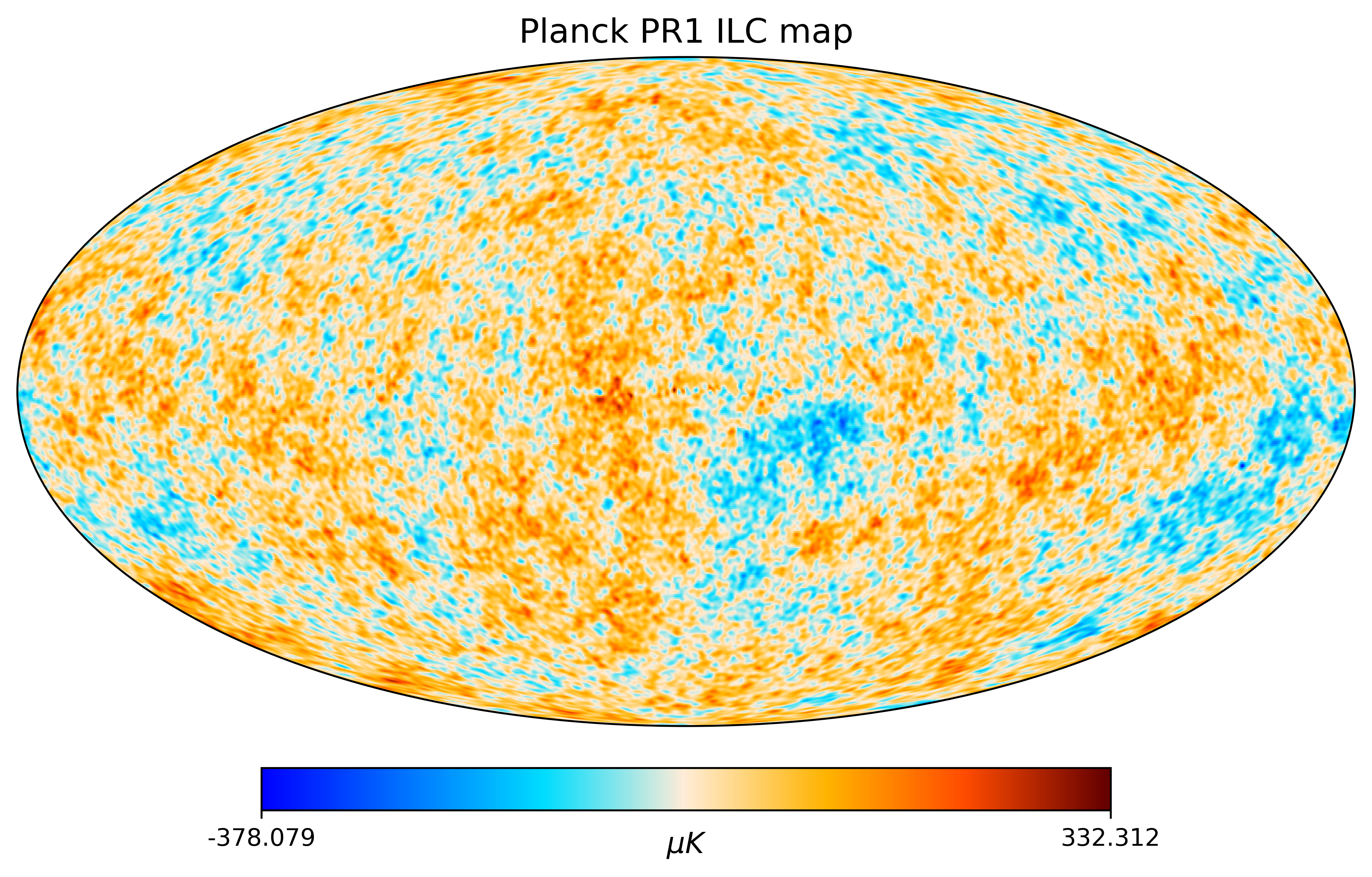
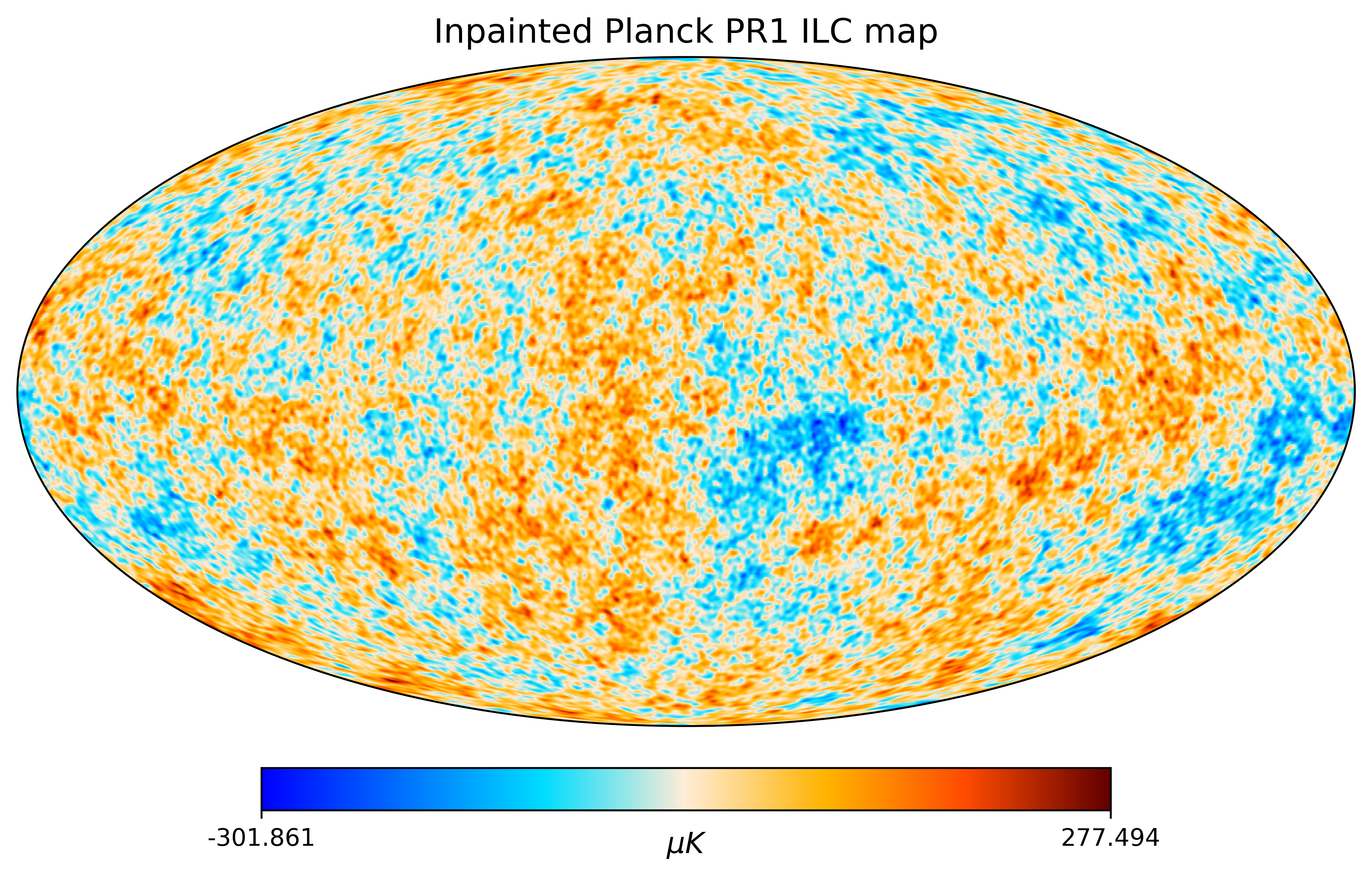
Figure 9: Cleaned CMB map obtained from Planck PR1 data using $30$ to $353~{}GHz$ channel maps, cleaned using internal linear combination (ILC) method is shown in the top panel. Same map inpainted using the mask depicted in Fig. [1] is shown in the bottom panel.

Once the smoothed noisy CMB frequency maps are obtained, these maps are combined using the same region specific internal linear combination (ILC) weights obtained from data. Thus, we generate 1000 such mock WILC maps corresponding to each data release from WMAP.

SMICA-like cleaned CMB maps from Planck satellite are provided as part of each data release by the Planck collaboration by processing the FFP simulations corresponding to each frequency channel in the same way as SMICA CMB map is obtained from observational data. SMICA map is provided at a higher resolution of  $N_{side}$=2048 with a Gaussian beam smoothing of $FWHM=5^{\prime}$. Hence these maps are repixelized following Eq. (15) to  $N_{side}$=512 and having a Gaussian beam of $FWHM=1^{\circ}$ (by taking $b_{l}^{\rm in}=b_{l}^{5^{\prime}}$, $b_{l}^{\rm out}=b_{l}^{1^{\circ}}$, $p_{l}^{\rm in}=p_{l}^{2048}$ and $p_{l}^{\rm out}=p_{l}^{512}$) similar to WILC maps.

Now to generate mock CMB maps for Planck’s PR1 data, the ILC weights used to clean the raw satellite maps from Planck PR1 are applied to the simulated FFP frequency realizations, iteratively, after processing them similar to data. We recall that Planck provided raw maps are available at  $N_{side}$=1024 for 30, 44, and 70 GHz bands (LFI bands) and at  $N_{side}$=2048 for 100, 143, 217, 353, 545 and 857 GHz bands (HFI bands). So they are brought to a common beam and pixel resolution of $1^{\circ}$ FWHM Gaussian beam and  $N_{side}$=512 respectively. Thus we generated 1000 mock PR1 ILC maps from the corresponding frequency specific FFP realizations. Note that we didn’t use the last two high frequency bands in obtaining Planck PR1 ILC CMB map.

We further note that WILC maps had a residual foregorund bias correction applied based on simulated foreground cleaned CMB maps Hinshaw et al. (2007b). However such a bias correction procedure was not employed on the CMB maps recoved using any of the four component separation methods (in real or harmonic space) used by the Planck collaboration.

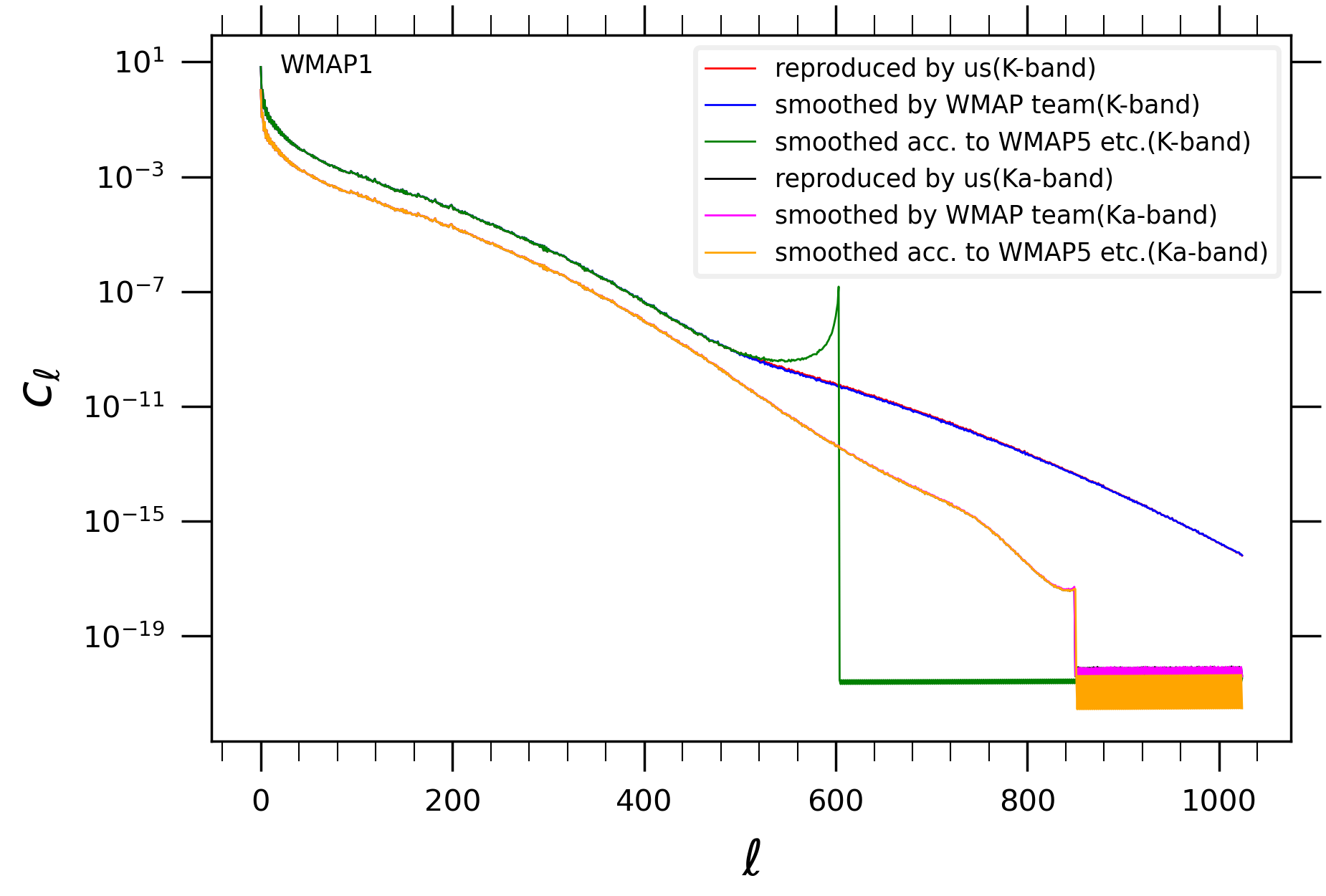
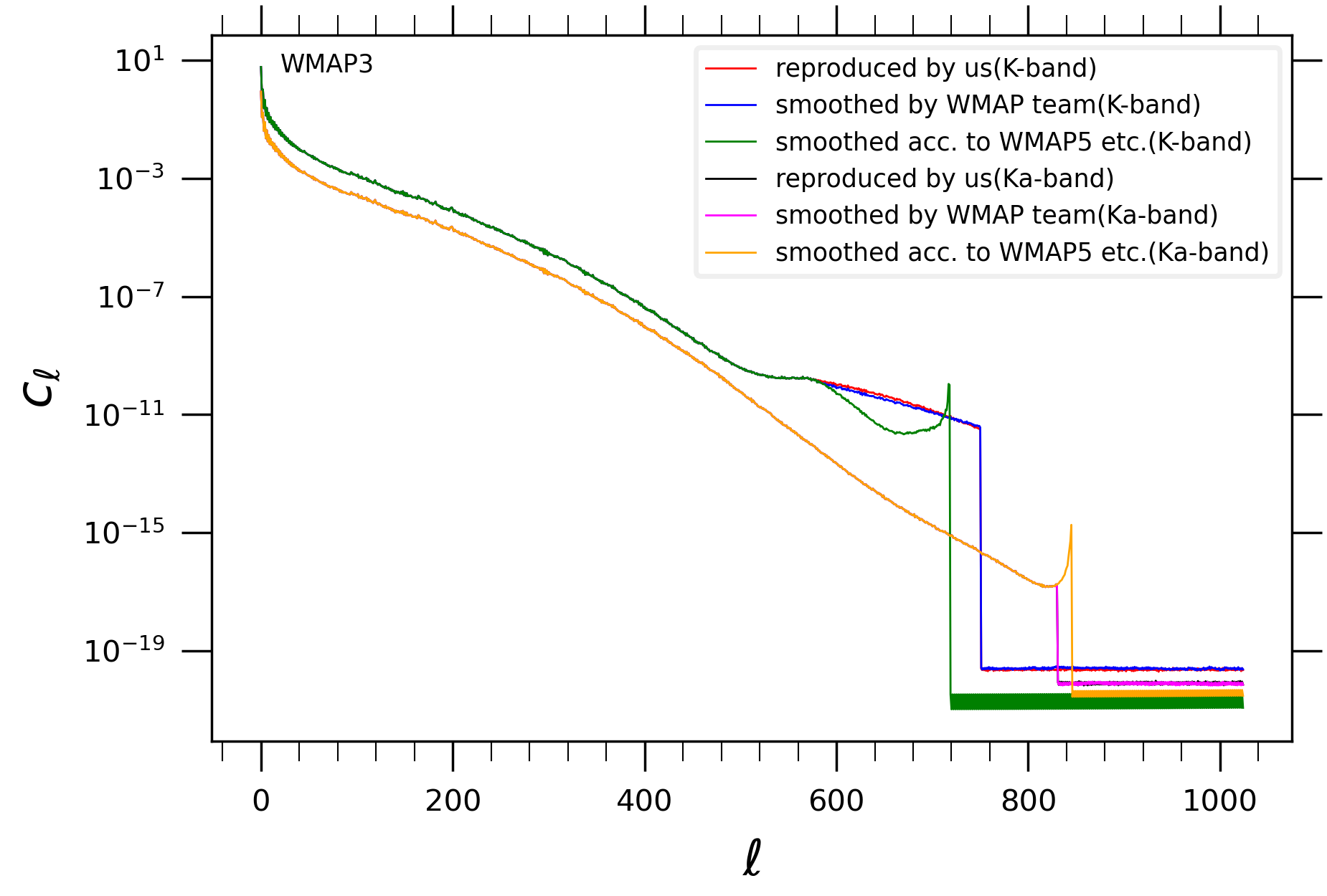
Figure 10: Power spectra of raw satellite maps from WMAP’s $K$ and $Ka$ bands provided by WMAP team as part of WMAP’s first and three year data products, and as obtained by us following Eq. (15).

Appendix B Masks used

The presence of residual foregrounds in the cleaned CMB maps can bias our inferences.Thus such regions of the sky are masked and inpainted using the iSAP package. However there will also be a bias introduced in the inpainted CMB maps if large fractions of the sky have to be inpainted. Since we are interested in CMB low multipoles, we use a single mask that has largely contiguous sky regions, but also masks extended regions with potential foreground residuals. It is obtained by combining WMAP’s nine year kp8 temperature cleaning mask and Planck’s 2018 common inpainting mask for temperature analysis as described below. WMAP’s nine year kp8 mask that is available at HEALPix  $N_{side}$=512 is upgraded to  $N_{side}$=2048 after removing small point sources from it. Then it is combined (multipled) with Planck 2018 common inpainting mask provided for intensity data. The combined mask thus obtained is then convolved with a Gaussian beam of $FWHM=1^{\circ}$ while deconvolving with a Gaussian beam of $FWHM=5^{\prime}$ following Eq. (15), and repixelized at  $N_{side}$=512. This combined smoothed mask is then thresholded such that those pixels which have a value $\geq 0.8$ are set to ‘$1$’ and rest are set to ‘$0$’. Mask thus obtained has a sky fraction of  $f_{sky}$$\approx 0.929$ which was shown in Fig. [1].

The data as well as simulated CMB maps corresponding to various data releases from WMAP and Planck missions are all inpainted using this mask.

Appendix C Smoothed $K$ and $Ka$ band maps from WMAP first and three year data release

There are few details to be noted in the generation of mock WILC CMB maps described in the previous section, and our observations while carrying out this analysis.

Since WMAP’s $K$ and $Ka$ frequency channel detectors are of low resolution, the effective circularized beam transfer functions ($b_{l}^{i}$) of these two bands were determined up to $l_{max}=750$ and $850$ respectively by the WMAP team. However, beam transfer functions provided cannot be used as such, since $K$-band $b_{l}$ from first year data are positive only up to $l=603$, and in three year data release $K$ and $Ka$ band $b_{l}$ are positive up to only $l=718$ and $845$ respectively. (Here, we also note that WMAP’s first year $Q$-band $b_{l}$ are provided only up to $l_{max}=1000$. Since the maps are being synthasized at  $N_{side}$=512, in general one uses mode information up to $l_{max}=2\times N_{side}$ when employing HEALPix i.e., $l_{max}=1024$ in our case.)

In order to perform ILC cleaning on raw satellite data, the individual frequency specific WMAP observed maps are synthesized at the same pixel resolution of  $N_{side}$=512 and a common beam smoothing given by a Gaussian kernal of $FWHM=1^{\circ}$ (which is slightly greater than the resolution of WMAP’s $K$-band detector’s effective Gaussian width). Since the input and output maps are at  $N_{side}$=512 in this case, $p_{l}^{\rm in}=p_{l}^{\rm out}$ in Eq. (15). The effective beam smoothing applied to each frequency map is then $b_{l}^{i,{\rm eff}}=b_{l}^{1^{\circ}}/b_{l}^{i}$. Thus in obtaining $1^{\circ}$ Gaussian beam smoothed raw maps, only the positive circularized $b_{l}^{i}$’s of $K$ and $Ka$ bands were used in computing $b_{l}^{i,{\rm eff}}$, and the rest were set to zero.

However this procedure seems to have been used from WMAP five year data analysis onwards uniformly for processing all frequency maps, but not in first and three year WMAP data analysis, especially $K$ and $Ka$ band maps. Our observations are presented in Fig. [10]. In the top panel, power spectrum plots of WMAP’s first year $1^{\circ}$ Gaussian beam smoothed $K$ and $Ka$ band maps as available from NASA’s LAMBDA site and their power spectrum as obtained by us following Eq. (15) are shown. Also shown are the power spectra of $K$ and $Ka$ band maps that are obtained using respective $b_{l}^{i}$ as given, but only up to some low multipole (i.e., not all positive $b_{l}^{i}$ were used), beyond which extrapolated $b_{l}^{i}$ are employed. These extrapolated $b_{l}^{i}$ are obtained by us, through trial and error, such that we are able to match the power spectra of smoothed $K$ and $Ka$ band maps thus obtained following Eq. (15), with the power spectra of smoothed $K$ and $Ka$ band maps as provided by WMAP team.

One readily notices that there is an artificial rise in the power at high mutlipoles when one uses Eq. (15) and all positive $b_{l}^{i}$ of $K$ and $Ka$ band maps as given. This could be the reason for using extrapolated $b_{l}^{i}$ by WMAP team for these two band maps in derving $1^{\circ}$ Gaussian beam smoothed raw maps that are eventually used in obtaining cleaned CMB map using ILC procedure. However these $b_{l}^{i,{\rm eff}}$ to get smoothed raw maps are not made publicly available to be able to appropriately simulate ILC-like maps from WMAP first and three years of observations.

The bottom panel of Fig. [10], is same as the top panel but corresponds to WMAP three year $K$ and $Ka$ band maps. We note that the rise in smoothed raw maps’ power is seen in $K$-band only in first year, and in both $K$ and $Ka$ band map powers in three year data owing to difference in fitted circularized beam transfer functions of corresponding detectors in the first and three year data analysis. These combination $b_{l}^{i}$ containing partly the circularized $b_{l}^{i}$ of $K$ and $Ka$ bands as provided and the extrapolated beam transfer function found by us (through trial and error) were used to simulate smoothed noisy frequency specific CMB maps to which ILC weights were applied in generating mock ILC cleaned CMB maps.

We were able to match the WMAP’s first year $1^{\circ}$ beam smoothed raw map as provided with the WMAP 1yr $K$-band map’s power spectrum by using $b_{l}^{K}$ up to $l=551$ as given, and fitting them using UnivariateSpline method of SciPy (a Python software library) choosing the degree of spline to be $k=2$ (i.e., using a quadratic spline) to obtain extrapolated $b_{l}^{K}$ up to $l=1024$. Then the extrapolated and given beam transfer functions of $K$-band are combined at $l=508$. Similarly, for WMAP’s 3yr $K$ band, we found (by trial and error) that interp1d method of SciPy with the paramter choice kind=‘slinear’ (first order/linear spline) gives extrapolated $b_{l}$ from $l=570$ onwards such that the combined $b_{l}$ result in a raw map power spectrum following Eq. (15) that matches with the smoothed raw maps’ $C_{l}$ from WMAP three year data. Thus combined $b_{l}$ up to a maximum multipole of $l=750$ were used for obtaining smoothed $K$ band map, and up to $l=830$ were used to get $Ka$ band smoothed map.

Appendix D Smoothed LFI maps from Planck PR1 data

We discussed the problem of appropriately simulating $1^{\circ}$ Gaussian beam smoothed maps corresponding to $K$ and $Ka$ bands that match with WMAP 1yr and 3yr smoothed $K$ and $Ka$ band data maps as provided by WMAP team in the previous section.

We face with a similar problem in trying to employ real space ILC method with Planck PR1 low frequency maps, specifically with the $30~{}GHz$ channel. Since we also chose to repixelize all the maps being used in the present study to  $N_{side}$=512 having a beam smoothing given by a Gaussian kernel with $FWHM=1^{\circ}$, Planck $30~{}GHz$ channel poses a similar problem. The circular beam transfer functions of all frequency maps from Planck 2013 data release are shown in Fig. [11].

It is clear from the figure that beam transfer functions of Planck’s $30~{}GHz$ PR1 frequency map as provided are not usable beyond $l\sim 850$ or so after which it shows an unphysical upward trend. Hence we adopt the same strategy as used for WMAP’s $K$ and $Ka$ band maps from its 1yr and 3yr data releases described in previous section i.e., to extrapolate $b_{l}$ of $30~{}GHz$ channel by using a suitable extrapolation scheme.

In particular, we fit the Planck PR1 $30~{}GHz$ channel’s $b_{l}$ as given for multipoles up to $l=860$. Then the beam transfer functions as provided up to $l=773$ are appended with the extrapolated $b_{l}$ obtained from the fit, where the two cross each other. The extrapolated $b_{l}$ were obtained by a fit to the given $b_{l}$ for $30~{}GHz$ detector using UnivariateSpline functionality of SciPy, a Python software library, with the paramter $k=2$ i.e., a quadratic spline. The effective (extrapolated) $b_{l}$ are generate up to $l=1100$ and following Eq. (15) Planck PR1 $30~{}GHz$ map was synthesized at  $N_{side}$=512 having $1^{\circ}$ Gaussian beam smoothing with mode information up to $l_{max}=1024$.

One can also see from Fig. [11] that the $40~{}GHz$ detector beam transfer function also shows a similar unphysical upward trend, but at a much higher multipole value. So, there was no need for such a procedure to repixelize freqeuncy maps other than $30~{}GHz$ channel map in obtaining ILC cleaned CMB map from Planck PR1 observed raw satellite maps at  $N_{side}$=512. Their beam transfer functions are well behaved up to $l=1024$ (that are needed for our purpose) for rest of the frequency maps.

We also note that this can be addressed in two other ways. As in WMAP 5yr and later data releases, $a_{lm}^{i}$’s of frequency maps in generating the smoothed maps can be set to zero for modes beyond that multipole for which $b_{l}$ are not provided or are not physically acceptable. A better way to address this is to use harmonic space ILC using only those modes ($a_{lm}^{i}$) from frequency channels where $b_{l}$ are available/acceptable to deconvolve the observed map for detector beam smoothing effects (see for example Tegmark et al. (2003)).

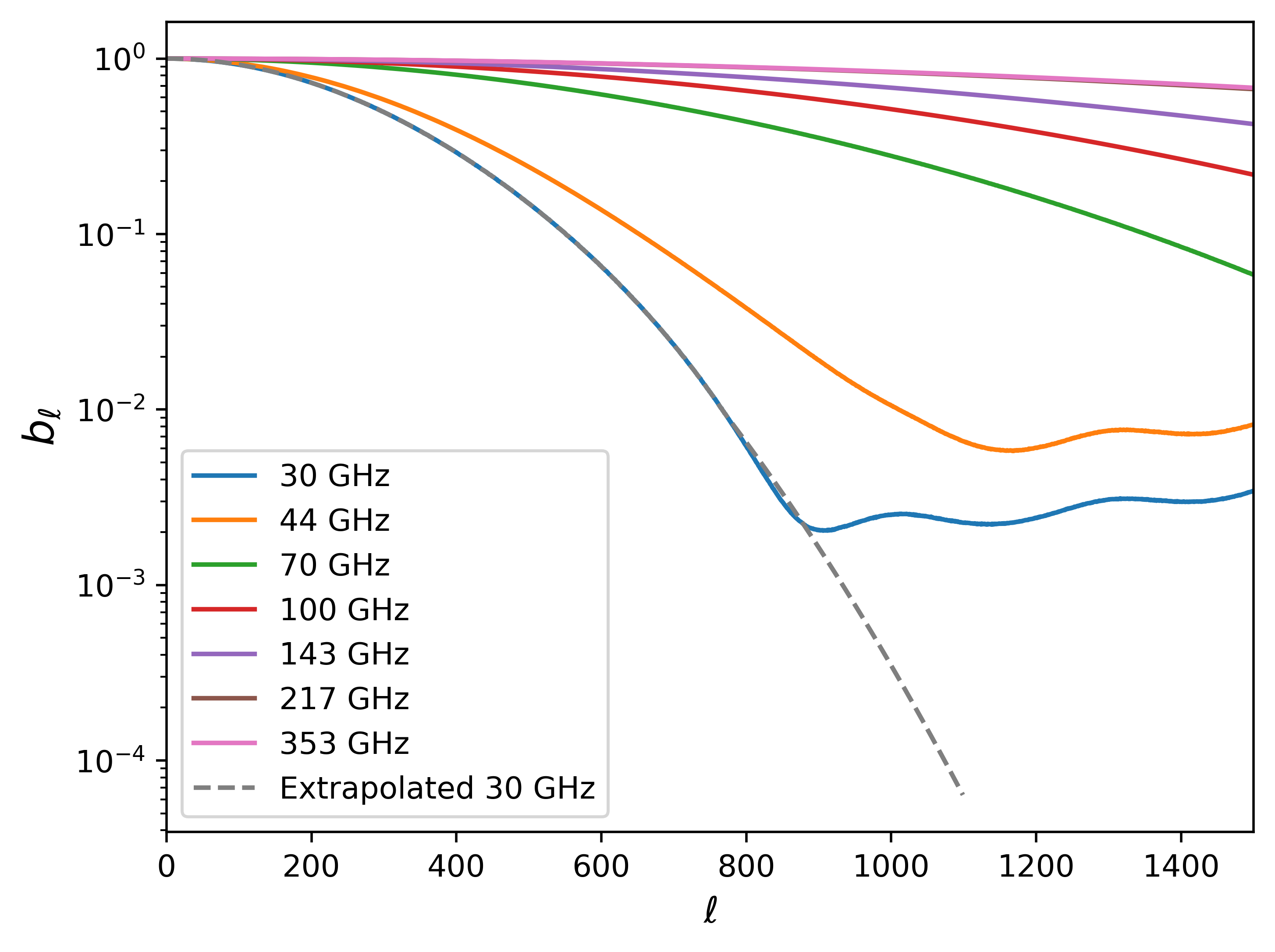
Figure 11: Circular beam transfer functions ($b_{l}$) of all frequency maps from Planck PR1 data. One can easily notice the unphysical upward trend of the $30~{}GHz$ channel’s effective circular $b_{l}$ as provided by Planck collaboration.

References

- Abramo et al. (2006) Abramo L. R., Bernui A., Ferreira I. S., Villela T., Wuensche C. A., 2006, Phys. Rev. D, 74, 063506
- Aluri et al. (2022) Aluri P. K., et al., 2022, arXiv e-prints, p. arXiv:2207.05765
- Bennett et al. (2003a) Bennett C. L., et al., 2003a, ApJS, 148, 1
- Bennett et al. (2003b) Bennett C. L., et al., 2003b, ApJS, 148, 97
- Bennett et al. (2011) Bennett C. L., et al., 2011, ApJS, 192, 17
- Bennett et al. (2013) Bennett C. L., et al., 2013, ApJS, 208, 20
- Bielewicz et al. (2004) Bielewicz P., Górski K. M., Banday A. J., 2004, MNRAS, 355, 1283
- Bielewicz et al. (2005) Bielewicz P., Eriksen H. K., Banday A. J., Górski K. M., Lilje P. B., 2005, ApJ, 635, 750
- Bull et al. (2016) Bull P., et al., 2016, Physics of the Dark Universe, 12, 56
- Cardoso et al. (2008) Cardoso J.-F., Le Jeune M., Delabrouille J., Betoule M., Patanchon G., 2008, IEEE Journal of Selected Topics in Signal Processing, 2, 735
- Copi et al. (2004) Copi C. J., Huterer D., Starkman G. D., 2004, Phys. Rev. D, 70, 043515
- Copi et al. (2006) Copi C. J., Huterer D., Schwarz D. J., Starkman G. D., 2006, MNRAS, 367, 79
- Copi et al. (2015) Copi C. J., Huterer D., Schwarz D. J., Starkman G. D., 2015, MNRAS, 449, 3458
- D’Agostino & Stephens (1986) D’Agostino R. B., Stephens M. A., 1986, Goodness-of-Fit Techniques. Marcel Dekker, Inc., USA
- Delabrouille et al. (2003) Delabrouille J., Cardoso J. F., Patanchon G., 2003, MNRAS, 346, 1089
- Eriksen et al. (2004) Eriksen H. K., Banday A. J., Górski K. M., Lilje P. B., 2004, ApJ, 612, 633
- Gold et al. (2009) Gold B., et al., 2009, ApJS, 180, 265
- Gold et al. (2011) Gold B., et al., 2011, ApJS, 192, 15
- Górski et al. (2005) Górski K. M., Hivon E., Banday A. J., Wandelt B. D., Hansen F. K., Reinecke M., Bartelmann M., 2005, ApJ, 622, 759
- Gruppuso & Gorski (2010) Gruppuso A., Gorski K. M., 2010, J. Cosmology Astropart. Phys., 2010, 019
- Harris et al. (2020) Harris C. R., et al., 2020, Nature, 585, 357
- Hinshaw et al. (2007a) Hinshaw G., et al., 2007a, ApJS, 170, 288
- Hinshaw et al. (2007b) Hinshaw G., et al., 2007b, ApJS, 170, 288
- Howlett et al. (2012) Howlett C., Lewis A., Hall A., Challinor A., 2012, J. Cosmology Astropart. Phys., 1204, 027
- Hunter (2007) Hunter J. D., 2007, Computing in Science & Engineering, 9, 90
- Land & Magueijo (2005) Land K., Magueijo J., 2005, Phys. Rev. Lett., 95, 071301
- Lewis et al. (2000) Lewis A., Challinor A., Lasenby A., 2000, ApJ, 538, 473
- Oliveira et al. (2020) Oliveira R. A., Pereira T. S., Quartin M., 2020, Physics of the Dark Universe, 30, 100608
- Pinkwart & Schwarz (2018) Pinkwart M., Schwarz D. J., 2018, Phys. Rev. D, 98, 083536
- Planck Collaboration et al. (2014) Planck Collaboration et al., 2014, A&A, 571, A23
- Planck Collaboration et al. (2016) Planck Collaboration et al., 2016, A&A, 594, A16
- Planck Collaboration et al. (2020) Planck Collaboration et al., 2020, A&A, 641, A7
- Ralston & Jain (2004) Ralston J. P., Jain P., 2004, International Journal of Modern Physics D, 13, 1857
- Samal et al. (2008) Samal P. K., Saha R., Jain P., Ralston J. P., 2008, MNRAS, 385, 1718
- Samal et al. (2009) Samal P. K., Saha R., Jain P., Ralston J. P., 2009, MNRAS, 396, 511
- Schwarz et al. (2004) Schwarz D. J., Starkman G. D., Huterer D., Copi C. J., 2004, Phys. Rev. Lett., 93, 221301
- Schwarz et al. (2016) Schwarz D. J., Copi C. J., Huterer D., Starkman G. D., 2016, Classical and Quantum Gravity, 33, 184001
- Starck et al. (2013) Starck J. L., Fadili M. J., Rassat A., 2013, A&A, 550, A15
- Tegmark et al. (2003) Tegmark M., de Oliveira-Costa A., Hamilton A. J., 2003, Phys. Rev. D, 68, 123523
- Virtanen et al. (2020) Virtanen P., et al., 2020, Nature Methods, 17, 261
- Zonca et al. (2020) Zonca A., Singer L., Lenz D., Reinecke M., Rosset C., Hivon E., Gorski K., 2020, healpy: Python wrapper for HEALPix, Astrophysics Source Code Library, record ascl:2008.022 (ascl:2008.022)
- de Oliveira-Costa et al. (2004) de Oliveira-Costa A., Tegmark M., Zaldarriaga M., Hamilton A., 2004, Phys. Rev. D, 69, 063516