Over-the-Air Majority Vote Computation with Modulation on Conjugate-Reciprocal Zeros
thanks: Alphan Şahin is with the Electrical Engineering Department, University of South Carolina, Columbia, SC, USA. E-mail: asahin@mailbox.sc.edu thanks: This paper was submitted in part to the IEEE Globel Communications Conference 2024 [1].

Alphan Şahin
Abstract

In this study, we propose a new approach to compute the MV function based on modulation on conjugate-reciprocal zeros (MOCZ) and introduce three different methods. The proposed methods rely on the fact that when a linear combination of polynomials is evaluated at one of the roots of a polynomial in the combination, that polynomial does contribute to the evaluation. To utilize this property, each transmitter maps the votes to the zeros of a Huffman polynomial, and the corresponding polynomial coefficients are transmitted. The receiver evaluates the polynomial constructed by the elements of the superposed sequence at conjugate-reciprocal zero pairs and detects the MV with a direct zero-testing (DiZeT) decoder. With differential and index-based encoders, we eliminate the need for power-delay information at the receiver while improving the computation error rate (CER) performance. The proposed methods do not use instantaneous channel state information at the transmitters and receiver. Thus, they provide robustness against phase and time synchronization errors. We theoretically analyze the CERs of the proposed methods. Finally, we demonstrate their efficacy in a distributed median computation scenario in a fading channel.

Index Terms:
Huffman polynomials, single-carrier waveform, over-the-air computation, zeros of polynomials

I Introduction

over-the-air computation (OAC) refers to the computation of special functions like arithmetic mean, norm, polynomial function, maximum, and MV by harnessing the signal superposition property of wireless multiple-access channels [2, 3, 4]. With OAC, instead of acquiring information from each device independently, the transmitters’ signals are intentionally overlapped on the same time-frequency resources to realize the summation operation as part of a desired function. Hence, OAC can improve resource utilization while reducing latency when the ultimate goal of communication is computation. With more applications relying on computation over wireless networks, OAC has recently been considered for a wide range of applications, such as wireless federated learning, distributed optimization, distributed localization, wireless data centers, and wireless control systems. We refer the readers to [5, 6, 7, 8, 9] and the references therein for further discussions in these areas. With this motivation, in this work, we propose a new OAC approach based on a recently proposed modulation technique, i.e., MOCZ [10, 11, 12], and introduce several methods to compute the MV function without CSI at the transmitters and receiver.

MOCZ is a non-linear modulation technique where information bits are encoded into the zeros of a polynomial, and the transmitted sequence corresponds to the polynomial coefficients [10]. As comprehensively analyzed in [11], the merit of MOCZ is that the zero structure of the transmitted signal is preserved at the receiver regardless of channel impulse response (CIR). This property is because the convolution operation can be represented as a polynomial multiplication, and the zeros are unaffected by the multiplication operation. As a result, MOCZ enables the receiver to obtain the information bits without the knowledge of instantaneous CSI. Although the idea of modulation on zeros can be used with an arbitrary set of polynomials, the zeros of a polynomial can be very sensitive to perturbation of its coefficients (e.g., Wilkinson’s polynomial [13]). To achieve robustness against additive noise, in [11], the authors propose to use Huffman polynomials [14], leading to binary modulation on conjugate-reciprocal zeros (BMOCZ). The zeros of a Huffman polynomial are evenly placed on two reciprocal circles centered at the origin. The angles of zeros uniformly divide 00 to $2\pi$ range, and their amplitudes can be either $d$ or $d^{-1}$ for $d>1$. The coefficients of the Huffman polynomials, i.e., Huffman sequences, are special in the sense that 1) their aperiodic auto-correlation functions are identical and very close to impulse function, and 2) their zeros are stable under additive noise. By using the conjugate-reciprocal zero structure of Huffman polynomials, the authors propose to encode an information bit into one of the zeros in a conjugate-reciprocal zero pair. A low-complexity non-coherent detector that compares two metrics by evaluating the polynomial constructed by the receive sequence at the zeros of a conjugate-reciprocal zero pair, i.e., DiZeT detector, is employed to detect the information bits without CSI.

In the literature, MOCZ is evaluated and improved in various scenarios. For instance, in [12], the authors investigate the practical aspects of MOCZ and assess its performance under impairments like carrier frequency and time offsets. In [15], MOCZ is investigated along with discrete Fourier transform-spread orthogonal frequency division multiplexing (DFT-s-OFDM) and extended to multi-user scenarios. In [16], the correlation properties of Huffman sequences are exploited to achieve joint radar and communications with MOCZ at 60 GHz millimeter wave band. In [17], the authors consider multiple antennas and develop a non-coherent Viterbi-like detector to achieve diversity gain. In [18], the authors consider an over-complete system for MOCZ based on faster-than-Nyquist signaling to improve spectral efficiency. To our knowledge, MOCZ has not been studied for OAC in the literature.

In practice, achieving a reliable computation with OAC is a difficult problem because the signal superposition occurs after the wireless channel distorts the signals. A commonly used approach is channel inversion at the transmitters where the transmitter multiplies the parameters with the inverses of the channel coefficients before transmission [19, 20, 21, 22]. While this solution ensures the receiver receives coherently superposed signals, it requires phase synchronization among the devices. However, phase synchronization can be very challenging in practice because of the inevitable hardware impairments such as clock errors, residual carrier frequency offset (CFO), and jittery time synchronization. For instance, a large phase rotation in the frequency domain can occur because of sample deviations at the transmitter or receiver [23]. Also, non-stationary channel conditions can deteriorate the coherent signal superposition in mobile environments [24]. To overcome the phase synchronization bottleneck, one solution is to use non-coherent energy accumulation based on type-based multiple access (TBMA) [25, 26]. The basic principle of TBMA is to estimate the frequency histogram to compute statistical averages by using orthogonal resources for different classes. For instance, in [27] and [28], two orthogonal resources representing the gradient directions (i.e., $1$ and $-1$ as votes) are allocated, and the norms of received symbols on these resources are compared to compute an MV function. Similarly, in [29], a decomposition based on a balanced number system is utilized to achieve a non-coherent quantized computation with TBMA. An alternative solution addressing the quantized nature of TBMA is modulating a sequence’s energy with the parameter to be aggregated [30, 31]. In this method, a random unimodular sequence is multiplied by the square root of the parameter. At the receiver, the norm-square of the received superposed sequence is calculated to estimate the aggregated parameter. Although Goldenbaum’s scheme can provide robustness against synchronization errors, it can suffer from interference terms due to the loss of orthogonality between the sequences. Nonetheless, non-coherent OAC schemes demonstrably work in practice without introducing stringent requirements. For instance, in [32], the aforementioned non-coherent MV computation is demonstrated for wireless federated learning with off-the-shelf software-defined radios. A similar strategy is also employed in [33] for separating values based on their signs. Also, Goldenbaum’s scheme is tested in practice in [34]. Given its robustness, we also consider non-coherent OAC in this work. Inspired by the features of MOCZ, we fundamentally strive to answer how the zeros of polynomials can be utilized for OAC without CSI at the transmitters and receiver.

I-A Contributions

Our contributions can be listed as follows:

  • We introduce a new approach to compute the MV function based on MOCZ. The fundamental property that we use is that when a linear combination of polynomials is evaluated at a specific value, and if this specific value corresponds to a root of a polynomial in the combinations, the contribution of that polynomial to the evaluation is zero. Based on this property, the transmitter chooses the zeros of Huffman’s polynomials based on its votes, i.e., $+1$ and $-1$, and the receiver evaluates the polynomial constructed with the elements of the superposed sequence at the corresponding zeros. With Lemma 1-3, we prove that the votes non-coherently superpose in a fading channel. We show that a DiZeT decoder, initially proposed for communications with MOCZ in [11], can also be used to obtain the MVs.

  • We propose three methods, each with its own advantages. While Method 1 provides the highest computation rate, it requires power-delay profile (PDP) information. We address this issue by using a differential encoding strategy in Method 2 at the expense of halved computation rate. Finally, by extending our preliminary results in [1], we reduce the CER by introducing redundancy in Method 3 with an index-based encoding, rigorously analyze the CERs of the proposed methods, and analytically derive the CERs in Corollaries 3-5 based on Lemma 4. All methods are robust to time and phase synchronization errors as they do not rely on the availability of CSI at the transmitters and receiver.

  • Finally, we support our findings with comprehensive simulations and assess each method’s CER and peak-to-mean envelope power ratio (PMEPR) distribution. We also demonstrate the applicability of the proposed method to a distributed median computation scenario. We also generate numerical results based on Goldenbaum’s OAC scheme in [30]. We demonstrate that the proposed methods can provide reliable MV computation in fading channels without any skewed behavior to the number of votes.

Organization: The rest of the paper is organized as follows. Section II provides the system model. In Section III, we discuss the proposed OAC methods in detail. In Section IV, we theoretically analyze the CERs of the proposed methods. In Section V, we provide numerical results and assess the methods in a distributed median computation scenario. We conclude the paper in Section VI.

Notation: The sets of complex and real numbers are denoted by $\mathbb{C}$ and $\mathbb{R}$, respectively. The function $\text{sign}\left(\cdot\right)$ results in $1$, $-1$, or 00 for a positive, a negative, or a zero-valued argument, respectively. $\mathbb{E}_{x}\left[\cdot\right]$ is the expectation of its argument over all random variables. The zero-mean circularly symmetric complex Gaussian distribution with variance $\sigma^{2}$ is denoted by $\mathcal{CN}({0,\sigma^{2}})$. The uniform distribution with the support between $a$ and $b$ is ${\mathcal{U}_{[a,b]}}$. The function $\mathbb{I}\left[{\cdot}\right]$ results in $1$ if its argument holds; otherwise, it is 00. The probability of an event $A$ is denoted by $\mathrm{Pr}({A;x})$, where $x$ is a parameter to calculate the probability.

II System Model

Consider an OAC scenario with $U$ transmitters and a receiver, where all radios are equipped with a single antenna. Let ${t}^{(u)}_{n}\in\mathbb{C}$ be a sample transmitted from the $u$th transmitter. Also, let $\textit{{h}}^{(u)}=(h^{(u)}_{0},\hbox to10.00002pt{.\hss.\hss.},h^{(u)}_{L-1})$ be the impulse response of the composite channel (including multipath channel and impairments like time and phase synchronization errors) between the $u$th transmitter and the receiver in discrete time, where $L\geq 1$ is the number of effective taps. Assume that all transmitters access the medium concurrently for computation. We can then express the $n$th received sample ${r}_{n}\in\mathbb{C}$ at the receiver after the signal superposition as

$\displaystyle{r}_{n}=\left(\sum_{u=1}^{U}\sum_{l=0}^{L-1}\sqrt{P_{u}}h^{(u)}_{l}{t}^{(u)}_{n-l}\right)+\omega_{n}~{},$ (1)

where $h^{(u)}_{l}\sim\mathcal{CN}({0,\rho_{l}})$ is the channel coefficient on the $l$th tap for the $u$th transmitter, $P_{u}$ is the average transmit power of the $u$th transmitter, and ${\omega_{n}}\sim\mathcal{CN}({0,\sigma_{\rm noise}^{2}})$ is the additive white Gaussian noise (AWGN). We consider an exponential decaying PDP for the channel between the $u$th transmitter and the receiver as

$\displaystyle\rho_{l}=\mathbb{E}\left[|h^{(u)}_{l}|^{2}\right]=\begin{cases}\frac{1-\rho}{1-\rho^{L}}\rho^{l}~{},&\rho<1\\ \frac{1}{L}~{},&\rho=1\end{cases}~{},$ (2)

for $\sum_{l=0}^{L-1}\rho_{l}=1$, where $\rho\in(0,1]$ is a decay constant [11]. We assume that the average received signal powers of the transmitters are aligned with a power control mechanism [35]. Thus, the relative positions of the transmitters to the receiver do not change our analyses as in [20, 21, 36]. Also, without loss of generality, we set $P_{u}$, $\forall u$, to $1$ Watt and calculate the average signal-to-noise ratio (SNR) of a transmitter at the receiver as ${\tt{SNR}}=1/\sigma_{\rm noise}^{2}$.

Let $\textit{{x}}^{(u)}=({x}^{(u)}_{0},{x}^{(u)}_{1},\dots,{x}^{(u)}_{K})$ denote the complex-valued coefficients of the polynomial function ${X^{(u)}}(z)={x}^{(u)}_{K}z^{K}+{x}^{(u)}_{K-1}z^{K-1}+\dots+{x}^{(u)}_{0}$ for $z\in\mathbb{C}$ and ${x}^{(u)}_{K}\neq 0$. We set ${t}^{(u)}_{n}$ as

$\displaystyle{t}^{(u)}_{n}=\begin{cases}{x}^{(u)}_{n},&0\leq n\leq K\\ 0,&\text{otherwise}\end{cases}.$ (3)

Since a convolution operation in discrete time can be represented by a polynomial multiplication in the $z$-domain, we can express the received sequence $\textit{{r}}=({r}_{0},\hbox to10.00002pt{.\hss.\hss.},{r}_{K+L-1})$ in (1) as

$\displaystyle{R}(z)$ $\displaystyle=\underbrace{\sum_{u=1}^{U}{X^{(u)}}(z){H^{(u)}}(z)}_{\triangleq{S}(z)}+{W}(z)~{},$ (4)

where ${W}(z)$ is the $z$-domain representation of the noise sequence $\textit{{w}}=({w}_{0},\hbox to10.00002pt{.\hss.\hss.},{w}_{K+L-1})$, and ${X^{(u)}}(z)$ and ${H^{(u)}}(z)$ are the $z$-domain representations of $\textit{{x}}^{(u)}$ and $\textit{{h}}^{(u)}$, respectively, i.e.,

$\displaystyle{X^{(u)}}(z)=\sum_{n=0}^{K}{x}^{(u)}_{n}z^{n}={x}^{(u)}_{K}\prod_{k=0}^{K-1}(z-\alpha^{(u)}_{k})~{},$ (5)

and

$\displaystyle{H^{(u)}}(z)=\sum_{l=0}^{L-1}h^{(u)}_{l}z^{l}=h^{(u)}_{L-1}\prod_{l=0}^{L-2}(z-\gamma^{(u)}_{l})~{},$ (6)

by using the facts that ${X^{(u)}}(z)$ and ${H^{(u)}}(z)$ have $K$ and $L-1$ complex-valued roots, respectively, by the fundamental theorem of algebra.

As in [11] and [12], in this study, we consider Huffman polynomials for ${X^{(u)}}(z)$ [14] and the roots of ${X^{(u)}}(z)$ are chosen as $\alpha^{(u)}_{k}\in\mathcal{Z}_{k}$, where $\mathcal{Z}_{k}=\{d{\rm e}^{\frac{{\rm j}2\pi k}{K}},d^{-1}{\rm e}^{\frac{{\rm j}2\pi k}{K}}\}$ consists of two conjugate-reciprocal complex numbers. Finally, we normalize $\lVert\textit{{x}}^{(u)}\rVert_{2}^{2}$ to $K+1$ by setting ${x}^{(u)}_{K}$ as

$\displaystyle{x}^{(u)}_{K}=\sqrt{\frac{\eta({K+1})}{\prod_{k=0}^{K-1}|\alpha^{(u)}_{k}|}}~{},$ (7)

for $\eta\triangleq{1}/({d^{K}+d^{-K}})$ and $d\triangleq\sqrt{1+\sin(\pi/K)}$ [11]. Note that this specific value of $d$ maximizes the minimum distance between the zeros.

II-A Problem Statement

Suppose that the fading coefficients, i.e., {$\textit{{h}}^{(u)}$, $\forall u$}, are not available at the transmitters and the receiver, and the receiver is interested in computing $M$ MV functions expressed as

$\displaystyle m_{\ell}=\text{sign}\left(\sum_{u=1}^{U}{v^{(u)}_{\ell}}\right)~{},\quad\forall\ell\in\{0,1,\hbox to10.00002pt{.\hss.\hss.},M-1\},$ (8)

where $v^{(u)}_{\ell}\in\{-1,1\}$ represents the $\ell$th vote of $u$th transmitter and $m_{\ell}\in\{-1,1\}$ is the $\ell$th MV. The fundamental challenge we address is how the MVs can be calculated by harnessing the signal superposition property of multiple-access channels while exploiting the concept of MOCZ while still being agnostic to CSI at the transmitters and receiver. Although MOCZ allows the receiver to use non-coherent detectors to obtain the bits for single-user communications, it is not trivial to use the same concept for computation in the channel as the signal superposition for $U>1$ in (4) destroys the original roots of the polynomials at the transmitters.

III Proposed Methods

In this section, we discuss three methods to compute MVs. Similar to BMOCZ in [11] and [12], we consider Huffman polynomials in the proposed methods. For their derivations, we need the following functions related to channel and noise:

$\displaystyle\Gamma(d)$ $\displaystyle\triangleq\mathbb{E}\left[|{{H^{(u)}}(d{\rm e}^{\frac{{\rm j}2\pi\ell}{K}})}|^{2}\right]=\sum_{l=0}^{L-1}\mathbb{E}\left[|h^{(u)}_{l}d^{l}{\rm e}^{\frac{{\rm j}2\pi\ell l}{K}}|^{2}\right]$
$\displaystyle=\sum_{l=0}^{L-1}\rho_{l}d^{2l}=\begin{cases}\frac{1-\rho}{1-\rho^{L}}\frac{1-d^{2L}\rho^{L}}{1-d^{2}\rho}~{},&\rho<1\\ \frac{1}{L}\frac{1-d^{2L}}{1-d^{2}}~{},&\rho=1\end{cases}~{}.$ (9)

and

$\displaystyle{\Omega}(d)\triangleq\mathbb{E}\left[\left|{{W}(d{\rm e}^{\frac{{\rm j}2\pi\ell}{K}})}\right|^{2}\right]=\sigma_{\rm noise}^{2}\frac{1-d^{2(K+L)}}{1-d^{2}}~{}.$ (10)

III-A Method 1: Uncoded MV Computation

In this method, we compute $M=K$ MVs without any coding and the $u$th transmitter sets the $k$th root of ${X^{(u)}}(z)$ based on the vote $v^{(u)}_{\ell}$, $\forall\ell\in\{0,1,\hbox to10.00002pt{.\hss.\hss.},K-1\}$, as

$\displaystyle\alpha^{(u)}_{k}$ $\displaystyle=\begin{cases}\frac{1}{d}{\rm e}^{\frac{{\rm j}2\pi k}{K}}\quad,&v^{(u)}_{k}=1\\ d{\rm e}^{\frac{{\rm j}2\pi k}{K}}\quad,&v^{(u)}_{k}=-1\\ \end{cases}~{}.$ (11)

The encoding in (11) is very similar to BMOCZ in [11]. However, since the transmitted signals superpose for OAC in (4), it is not trivial how to design the detector to detect the MVs. We use the following lemma to develop the decoder:

Lemma 1.

Let $U^{+}_{\ell}$ and $U^{-}_{\ell}$ denote the number of transmitters with positive and negative votes for $\ell$th MV computation. For the mapping in (11) with $\mathrm{Pr}({v^{(u)}_{\ell^{\prime}}=1})=\mathrm{Pr}({v^{(u)}_{\ell^{\prime}}=-1})=1/2$, $\forall\ell^{\prime}$, $\ell^{\prime}\neq\ell$,

$\displaystyle\mathbb{E}\left[\left|{{S}(d{\rm e}^{\frac{{\rm j}2\pi\ell}{K}})}\right|^{2}\right]$ $\displaystyle=U^{+}_{\ell}\mathcal{X}_{1}(d)\Gamma(d)~{},$ (12)

where

$\displaystyle\mathcal{X}_{1}(d)\triangleq\eta({K+1})(d-d^{-1})^{2}d^{{K}}$
$\displaystyle~{}~{}~{}~{}~{}~{}~{}\times\frac{1}{2^{K-1}}\prod_{\begin{subarray}{c}k=1\end{subarray}}^{K-1}{{|1-{\rm e}^{\frac{{\rm j}2\pi k}{K}}|^{2}}+{|d-d^{-1}{\rm e}^{\frac{{\rm j}2\pi k}{K}}|^{2}}}~{},$ (13)

where the expectations in (12) over the distributions of channels and votes.

The proof is given in Appendix A.

Corollary 1.

$\mathbb{E}\left[{{S}(d^{-1}{\rm e}^{\frac{{\rm j}2\pi\ell}{K}})}\right]$ can be calculated by replacing with $U^{+}_{\ell}$ and $d$ with $U^{-}_{\ell}$ and $d^{-1}$ in (12), respectively.

The key observation from Lemma 1 and Corollary 1 is that the expected values of ${{S}(d{\rm e}^{\frac{{\rm j}2\pi\ell}{K}})}$ and ${{S}(d^{-1}{\rm e}^{\frac{{\rm j}2\pi\ell}{K}})}$ are linearly scaled by $U^{+}_{\ell}$ and $U^{-}_{\ell}$, respectively. Thus, a DiZeT decoder, initially used for detecting bits [11], can still be utilized for computing the $\ell$th MV with proper scaling coefficients highlighted by Lemma 1 and Corollary 1 as

$\displaystyle\hat{m}_{\ell}=\operatorname{sign}{(\tilde{U}^{+}_{\ell}-\tilde{U}^{-}_{\ell})}~{},$ (14)

where $\tilde{U}^{+}_{\ell}$ and $\tilde{U}^{-}_{\ell}$ are the unbiased estimates of $U^{+}_{\ell}$ and $U^{-}_{\ell}$, respectively, given by

$\displaystyle\tilde{U}^{+}_{\ell}=\frac{\left|{{R}(d{\rm e}^{\frac{{\rm j}2\pi\ell}{K}})}\right|^{2}-{\Omega}(d)}{\mathcal{X}_{1}(d)\Gamma(d)}~{},$ (15)

and

$\displaystyle\tilde{U}^{-}_{\ell}=\frac{\left|{{R}(d^{-1}{\rm e}^{\frac{{\rm j}2\pi\ell}{K}})}\right|^{2}-{\Omega}(d^{-1})}{\mathcal{X}_{1}(d^{-1})\Gamma(d^{-1})}~{}.$ (16)

Note that (14) can be simplified by using ${\mathcal{X}_{1}(d)}/{\mathcal{X}_{1}(d^{-1})}=d^{2K}$, but it still requires the PDP of the channel.

The computation rate for Method 1 can also obtained as $K$ MVs over $K+L$ complex-valued resources. The number of consumed resources is $K+L$ as the transmitted sequence needs to be padded with $L$ zeros to express (4).

III-B Method 2: Differential MV Computation

In this method, we consider a differential encoding to compute $M=K/2$ MVs and the $u$th transmitter sets the $k$th and $(k+1)$th roots of ${X^{(u)}}(z)$ based on the vote $v^{(u)}_{\ell}$, $\forall\ell\in\{0,1,\hbox to10.00002pt{.\hss.\hss.},K/2-1\}$, as

$\displaystyle(\alpha^{(u)}_{2k^{\prime}},\alpha^{(u)}_{2k^{\prime}+1})$ $\displaystyle=\begin{cases}(\frac{1}{d}{\rm e}^{\frac{{\rm j}2\pi 2k^{\prime}}{K}},d{\rm e}^{\frac{{\rm j}2\pi(2k^{\prime}+1)}{K}}),&v^{(u)}_{k^{\prime}}=1\\ (d{\rm e}^{\frac{{\rm j}2\pi 2k^{\prime}}{K}},\frac{1}{d}{\rm e}^{\frac{{\rm j}2\pi(2k^{\prime}+1)}{K}}),&v^{(u)}_{k^{\prime}}=-1\\ \end{cases}~{}.$ (17)

for $k^{\prime}=\lfloor{k}/{2}\rfloor$. To derive the detector for this encoder, we use the following lemma:

Lemma 2.

Let $U^{+}_{\ell}$ and $U^{-}_{\ell}$ denote the number of transmitters with positive and negative votes for $\ell$th MV computation. For the mapping in (17) with $\mathrm{Pr}({v^{(u)}_{\ell^{\prime}}=1})=\mathrm{Pr}({v^{(u)}_{\ell^{\prime}}=-1})=1/2$, $\forall\ell^{\prime}$, $\ell^{\prime}\neq\ell$,

$\displaystyle\mathbb{E}\left[\left|{{S}(d{\rm e}^{\frac{{\rm j}2\pi 2\ell}{K}})}\right|^{2}\right]$ $\displaystyle=U^{+}_{\ell}\mathcal{X}_{2}(d)\Gamma(d)~{},$ (18)

where

$\displaystyle\mathcal{X}_{2}(d)\triangleq\eta({K+1})(d-d^{-1})^{2}|1-{\rm e}^{\frac{2\pi}{K}}|^{2}d^{K}$
$\displaystyle~{}~{}~{}~{}~{}~{}\times\frac{1}{2^{\frac{K}{2}-1}}\prod_{\begin{subarray}{c}k=1\end{subarray}}^{\frac{K}{2}-1}{{|1-{\rm e}^{\frac{{\rm j}2\pi 2k}{K}}|^{2}}}{{|d-d^{-1}{\rm e}^{\frac{{\rm j}2\pi(2k+1)}{K}}|^{2}}}$
$\displaystyle~{}~{}~{}~{}~{}~{}~{}~{}~{}~{}~{}~{}~{}~{}~{}~{}~{}~{}~{}~{}+{|1-{\rm e}^{\frac{{\rm j}2\pi(2k+1)}{K}}|^{2}}{{|d-d^{-1}{\rm e}^{\frac{{\rm j}2\pi 2k}{K}}|^{2}}}~{},$ (19)

where the expectation in (18) over the distributions of channels and votes.

The proof is given in Appendix B.

Corollary 2.

$\mathbb{E}\left[{{S}(d{\rm e}^{\frac{{\rm j}2\pi(2\ell+1)}{K}})}\right]$ can be calculated by replacing $U^{+}_{\ell}$ with $U^{-}_{\ell}$ in (18).

With, the unbiased estimates of $U^{+}_{\ell}$ and $U^{-}_{\ell}$ can be obtained as

$\displaystyle\tilde{U}^{+}_{\ell}=\frac{\left|{{R}(d{\rm e}^{\frac{{\rm j}2\pi 2\ell}{K}})}\right|^{2}-{\Omega}(d)}{\mathcal{X}_{2}(d)\Gamma(d)}~{},$ (20)

and

$\displaystyle\tilde{U}^{-}_{\ell}=\frac{\left|{{R}(d{\rm e}^{\frac{{\rm j}2\pi(2\ell+1)}{K}})}\right|^{2}-{\Omega}(d)}{\mathcal{X}_{2}(d)\Gamma(d)}~{},$ (21)

respectively. Hence, the $\ell$th MV can be computed as

$\displaystyle\hat{m}_{\ell}=$ $\displaystyle\text{sign}\left(\left|{{R}(d{\rm e}^{\frac{{\rm j}2\pi(2\ell+1)}{K}})}\right|^{2}-\left|{{R}(d{\rm e}^{\frac{{\rm j}2\pi 2\ell}{K}})}\right|^{2}\right).$ (22)

Compared with the detector in Method 1, the detector in (22) does not need the PDP of the channel to compute the MVs. The price paid for this benefit is a reduced computation rate, i.e., $K/2$ MVs over $K+L$ complex-valued resources.

III-C Method 3: Index-based MV Computation

In this approach, we compute $M=\log_{2}(K)$ MVs, and the roots of ${X^{(u)}}(z)$ are modulated based on an index calculated by using all votes. To this end, let $b^{(u)}_{\ell}\in\mathbb{Z}_{2}$ be a binary representation of the vote $v^{(u)}_{\ell}$ as $b^{(u)}_{\ell}\triangleq(v^{(u)}_{\ell}+1)/2$ for $\forall\ell\in\{0,1,\hbox to10.00002pt{.\hss.\hss.},\log_{2}(K)-1\}$. The $u$th transmitter sets the $k$th root of ${X^{(u)}}(z)$ as

$\displaystyle\alpha^{(u)}_{k}$ $\displaystyle=\begin{cases}\frac{1}{d}{\rm e}^{\frac{{\rm j}2\pi k}{K}},&\sum_{\ell=0}^{M-1}b^{(u)}_{\ell}2^{\ell}=k\\ d{\rm e}^{\frac{{\rm j}2\pi k}{K}},&\text{otherwise}\\ \end{cases}~{}.$ (23)

For instance, we obtain $\sum_{\ell=0}^{M-1}b^{(u)}_{\ell}2^{\ell}=0$ for $v^{(u)}_{\ell}=-1$, $\forall\ell$, as $b^{(u)}_{\ell}=0$, $\forall\ell$. Hence, the radius of the 00th root is set to $d^{-1}$, while the radius of any other root for $k\neq 0$ is determined as $d$.

Lemma 3.

Let $U^{+}_{\ell}$ and $U^{-}_{\ell}$ denote the number of transmitters with positive and negative votes for $\ell$th MV computation. For the mapping in (23) with $\mathrm{Pr}({v^{(u)}_{\ell^{\prime}}=1})=\mathrm{Pr}({v^{(u)}_{\ell^{\prime}}=-1})=1/2$, $\forall\ell^{\prime}$ and $\ell^{\prime}\neq\ell$,

$\displaystyle\mathbb{E}\left[\left|{{S}(d{\rm e}^{\frac{{\rm j}2\pi l}{K}})}\right|^{2}\right]$ $\displaystyle=\frac{U^{+}_{\ell}\mathbb{I}\left[{l_{\ell}=1}\right]+U^{-}_{\ell}\mathbb{I}\left[{l_{\ell}=0}\right]}{2^{\log_{2}({K})-1}}\mathcal{X}_{3}(d)\Gamma(d)~{},$ (24)

where

$\displaystyle\mathcal{X}_{3}(d)\triangleq\eta({K+1})(d-d^{-1})^{2}d^{K}K^{2}$ (25)

where the expectations in (24) over the distributions of channels and votes and $l=\sum_{i=0}^{M-1}l_{i}2^{i}$ with $l_{i}\in\mathbb{Z}_{2}$, $\forall i$.

The proof is given in Appendix C.

Based on Lemma 3, we can obtain unbiased estimates of $U^{+}_{\ell}$ and $U^{-}_{\ell}$ as

$\displaystyle\tilde{U}^{+}_{\ell}=\frac{\sum_{\begin{subarray}{c}l=0,l_{\ell}=1\end{subarray}}^{K-1}\left|{{R}(d{\rm e}^{\frac{{\rm j}2\pi l}{K}})}\right|^{2}-\frac{K}{2}{\Omega}(d)}{\mathcal{X}_{2}(d)\Gamma(d)2^{-\log_{2}({K})+1}}~{},$ (26)

and

$\displaystyle\tilde{U}^{-}_{\ell}=\frac{\sum_{\begin{subarray}{c}l=0,l_{\ell}=0\end{subarray}}^{K-1}\left|{{R}(d{\rm e}^{\frac{{\rm j}2\pi l}{K}})}\right|^{2}-\frac{K}{2}{\Omega}(d)}{\mathcal{X}_{2}(d)\Gamma(d)2^{-\log_{2}({K})+1}}~{},$ (27)

respectively, and derive the detector to obtain the $\ell$th MV as

$\displaystyle\hat{m}_{\ell}=$ $\displaystyle\text{sign}\left(\sum_{\begin{subarray}{c}l=0\\ l_{\ell}=1\end{subarray}}^{K-1}\left|{{R}(d{\rm e}^{\frac{{\rm j}2\pi l}{K}})}\right|^{2}-\sum_{\begin{subarray}{c}l=0\\ l_{\ell}=0\end{subarray}}^{K-1}\left|{{R}(d{\rm e}^{\frac{{\rm j}2\pi l}{K}})}\right|^{2}\right).$ (28)

Compared with Method 1 and Method 2, Method 3 uses $K/2$ measurements for each test in (28) to determine the MVs. Hence, as demonstrated in Section V, it yields a better CER at the expense of a lower computation rate, i.e., $\log_{2}(K)$ MVs over $K+L$ complex-valued resources. Also, the detector does not use the PDP. Note that Method 3 reduces to Method 2 for $K=2$.

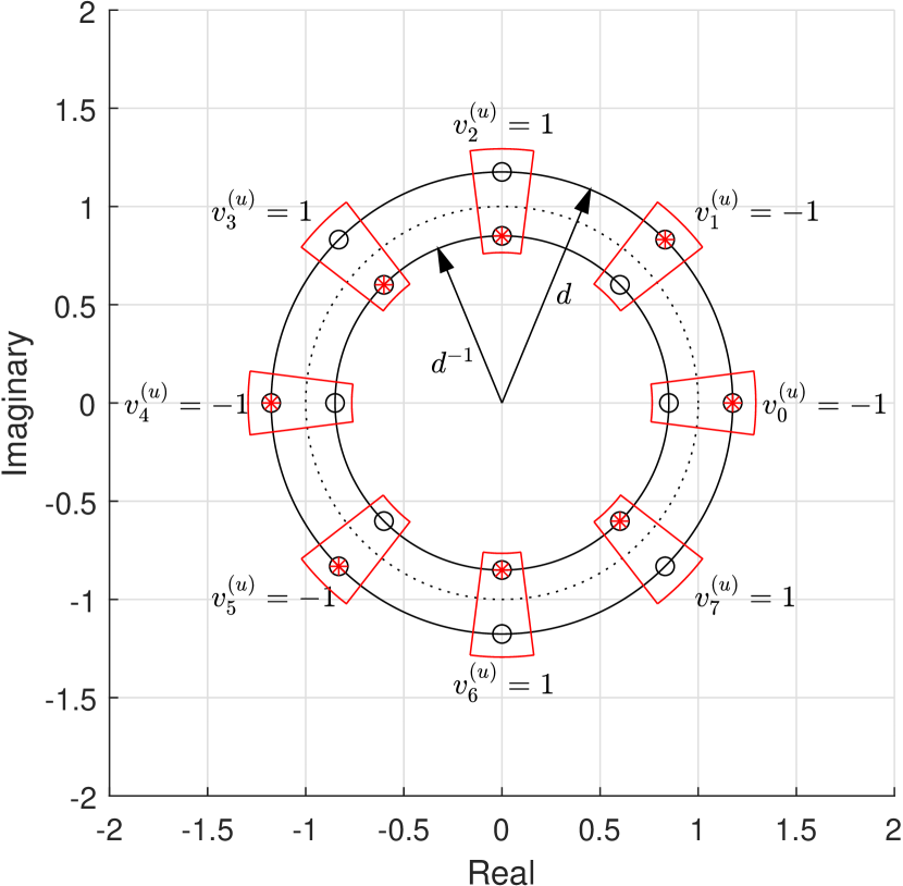
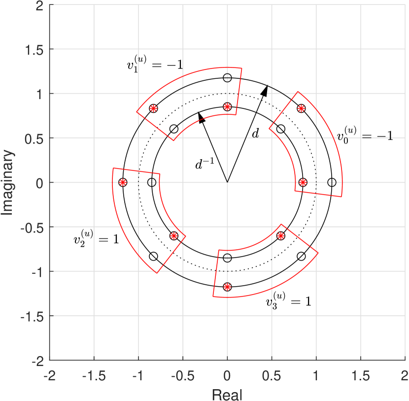
In Figure 1, we exemplify the zero placements for Methods 1-3 and $K=8$. In Figure 1LABEL:sub@subfig:example1, we assume that the votes at the transmitter are $(v^{(u)}_{0},\hbox to10.00002pt{.\hss.\hss.},v^{(u)}_{7})=(-1,-1,1,1,-1,-1,1,1)$. By following (11), the zeros (see the points marked by stars in Figure 1LABEL:sub@subfig:example1) are chosen based on the values of $v^{(u)}_{\ell}$. In Figure 1LABEL:sub@subfig:example2, we consider Method 2, and the votes are $(v^{(u)}_{0},v^{(u)}_{1},v^{(u)}_{2},v^{(u)}_{3})=(-1,-1,1,1)$. In this method, two zeros are allocated for each vote, and the zeros alternate their radii based on the value of the vote by (17). Finally, in Figure 1LABEL:sub@subfig:example3, we show the zero placement for Method 3 for $(v^{(u)}_{0},v^{(u)}_{1},v^{(u)}_{2})=(-1,1,-1)$. Since we obtain $\sum_{\ell=0}^{M-1}b^{(u)}_{\ell}2^{\ell}=2$ for $(b^{(u)}_{0},b^{(u)}_{1},b^{(u)}_{2})=(0,1,0)$ from (23), the zero indexed by $k=2$ changes its position while the other zeros remain on the circle with the radius $d$.

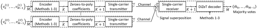
Finally, we provide the transmitter and receiver block diagrams in Figure 2. After the encoder generates the zeros, i.e., a zero codeword of length $K$, the zero codeword is converted to polynomial coefficients of length $K+1$. In Appendix D, we provide how the zeros can be converted to the polynomial coefficients by using discrete Fourier transform (DFT). Note that an iterative algorithm discussed in [11, Eq. (8)] can also be used for this conversion.111The MATLAB’s $\mathtt{poly}$ function also uses the iterative algorithm discussed in [11, Eq. (8)]. However, based on our analysis, $\mathtt{poly}$ function does not provide stable results for large $K$ values. We use the implementation based on the derivation in Appendix D. After the conversion, the polynomial coefficients are transmitted with a single-carrier transmitter (e.g., upsampling and pulse shaping). We refer the reader to [37] for the variants of a single-carrier waveform. The receiver receives the sum of the transmitted signals after they pass through independent channels. After processing the superposed signal with a single-carrier receiver (e.g., matched filter and down-sampling), the receiver uses a DiZeT decoder, i.e., (14), (22), or (28), to obtain the MVs.

Refer to caption
(a) Method 1 - Uncoded.
Refer to caption
(b) Method 2 - Differential encoder.
Refer to caption
(c) Method 3 - Index-based encoder.
Figure 1: Example zero placements for Methods 1-3. The star and circle markers indicate the chosen zeros and the possible zero locations for a Huffman polynomial, respectively.
Refer to caption
Figure 2: Transmitter and receiver block diagrams.

IV Computation-error rate Analysis

For Methods 1-3, we can express the CER for the $\ell$th MV as

$\displaystyle{\tt{CER}}_{\ell}=\begin{cases}\mathrm{Pr}({\tilde{U}^{+}_{\ell}-\tilde{U}^{-}_{\ell}<0})~{},&U^{+}_{\ell}>U^{-}_{\ell}\\ 1-\mathrm{Pr}({\tilde{U}^{+}_{\ell}-\tilde{U}^{-}_{\ell}<0})~{},&U^{+}_{\ell}<U^{-}_{\ell}\\ 1~{},&U^{+}_{\ell}=U^{-}_{\ell}\end{cases}~{},$ (29)

where the third case in (29) is because $\operatorname{sign}({\tilde{U}^{+}_{\ell}-\tilde{U}^{-}_{\ell}})$ is almost surely not zero due to the noisy reception in communication channels. We can also express $\mathrm{Pr}({\tilde{U}^{+}_{\ell}-\tilde{U}^{-}_{\ell}<0})$ as

$\displaystyle\mathrm{Pr}({\tilde{U}^{+}_{\ell}-\tilde{U}^{-}_{\ell}<0})$ $\displaystyle=\mathbb{E}_{\dot{\textit{{{V}}}}}\left[F_{\tilde{U}^{+}_{\ell}-\tilde{U}^{-}_{\ell}}\left({x;\textit{{{V}}}}\right)\right]$
$\displaystyle=\frac{1}{2^{M(U-1)}}\sum_{\forall\dot{\textit{{{V}}}}}{F_{\tilde{U}^{+}_{\ell}-\tilde{U}^{-}_{\ell}}\left({x;\textit{{{V}}}}\right)}]~{},$ (30)

where $F_{\tilde{U}^{+}_{\ell}-\tilde{U}^{-}_{\ell}}\left({x;\textit{{{V}}}}\right)$ is the cumulative distribution function (CDF) of $\tilde{U}^{+}_{\ell}-\tilde{U}^{-}_{\ell}$ given all votes $\textit{{{V}}}\triangleq(\textit{{u}}_{\ell},\dot{\textit{{{V}}}})$ for $\textit{{u}}_{\ell}={({{\mathbf{1}}}_{U^{+}_{\ell}},-{{\mathbf{1}}}_{U^{-}_{\ell}})}$ and $\dot{\textit{{{V}}}}\triangleq(\textit{{u}}_{1},\hbox to10.00002pt{.\hss.\hss.},\textit{{u}}_{\ell-1},\textit{{u}}_{\ell+1},\hbox to10.00002pt{.\hss.\hss.},\textit{{u}}_{U})$. Hence, we need an analytical expression of $F_{\tilde{U}^{+}_{\ell}-\tilde{U}^{-}_{\ell}}\left({0;\textit{{{V}}}}\right)$ to obtain $\mathrm{Pr}({\tilde{U}^{+}_{\ell}-\tilde{U}^{-}_{\ell}<0})$. To this end, we use the following result from [38]:

Lemma 4 ([38]).

Let $a_{l}$ and $b_{l}$ be independent exponential random variables with the rate $\lambda_{a_{l}}$ and $\lambda_{b_{l}}$, respectively, $\forall l\in\{0,\hbox to10.00002pt{.\hss.\hss.}K-1\}$. For $A=\sum_{l=0}^{K-1}a_{l}$ and $B=\sum_{l=0}^{K-1}b_{l}$, $F_{A-B}\left({x}\right)$ can be calculated as

$\displaystyle F_{A-B}\left({x}\right)$ $\displaystyle=\frac{1}{2}-\int_{-\infty}^{\infty}\frac{\varphi_{a}(t){{\varphi}_{b}^{*}(t)}}{2\pi{\rm j}t}{\rm e}^{-{\rm j}tx}dt~{},$ (31)

where

$\displaystyle\varphi_{a}(t)=\prod_{{l=0}}^{K-1}\frac{1}{1-{\rm j}t{\lambda_{a_{l}}}^{-1}}~{},$ (32)

and

$\displaystyle\varphi_{b}(t)=\prod_{{l=0}}^{K-1}\frac{1}{1-{\rm j}t\lambda_{b_{l}}^{-1}}~{}.$ (33)

Lemma (4) exploits the characteristic functions of the exponential distribution, convolution theorem, and the inversion formula given in [39]. We can now calculate the $F_{\tilde{U}^{+}_{\ell}-\tilde{U}^{-}_{\ell}}\left({0;\textit{{{V}}}}\right)$ for Methods 1-3 theoretically as follows:

Corollary 3.

$F_{\tilde{U}^{+}_{\ell}-\tilde{U}^{-}_{\ell}}\left({0;\textit{{{V}}}}\right)$ for Method 1 can be calculated by evaluating (31) at $x={{\Omega}(d)}/({\mathcal{X}_{1}(d)\Gamma(d)})-{{\Omega}(d^{-1})}/({\mathcal{X}_{1}(d^{-1})\Gamma(d^{-1})})$ for

$\displaystyle\varphi_{a}(t)=\frac{1}{1-{\rm j}t\lambda_{+}^{-1}}~{},$ (34)

and

$\displaystyle\varphi_{b}(t)=\frac{1}{1-{\rm j}t\lambda_{-}^{-1}}~{},$ (35)

with

$\displaystyle\lambda_{+}^{-1}=\frac{1}{\mathcal{X}_{1}(d)}\sum_{u=1}^{U}|{X^{(u)}}(d{\rm e}^{\frac{{\rm j}2\pi l}{K}})|^{2}+\frac{{\Omega}(d)}{\mathcal{X}_{1}(d)\Gamma(d)}~{},$

and

$\displaystyle\lambda_{-}^{-1}=\frac{1}{\mathcal{X}_{1}(d^{-1})}\sum_{u=1}^{U}|{X^{(u)}}(d^{-1}{\rm e}^{\frac{{\rm j}2\pi l}{K}})|^{2}+\frac{{\Omega}(d^{-1})}{\mathcal{X}_{1}(d^{-1})\Gamma(d^{-1})}~{}.$
Corollary 4.

$F_{\tilde{U}^{+}_{\ell}-\tilde{U}^{-}_{\ell}}\left({0;\textit{{{V}}}}\right)$ for Method 3 can be calculated by evaluating (31) at $x=0$ with

$\displaystyle\varphi_{a}(t)=\prod_{\begin{subarray}{c}l=0\\ l_{\ell}=1\end{subarray}}^{K-1}\frac{1}{1-{\rm j}t\lambda_{l}^{-1}}~{},$ (36)

and

$\displaystyle\varphi_{b}(t)=\prod_{\begin{subarray}{c}l=0\\ l_{\ell}=0\end{subarray}}\frac{1}{1-{\rm j}t\lambda_{l}^{-1}}~{},$ (37)

for $\lambda_{l}^{-1}=\Gamma(d)\sum_{u=1}^{U}|{X^{(u)}}(d{\rm e}^{\frac{{\rm j}2\pi l}{K}})|^{2}+{\Omega}(d)$.

The proofs of Corollary 3 and Corollary 4 are deferred to Appendix E.

Corollary 5.

Since Method 3 reduces to Method 2 for $K=2$, the CER for Method 2 can be also directly calculated by using Corollary (4).

It is worth emphasizing that the integral in (31) can be evaluated numerically for a given set of rate values for Methods 1-3. Also, the sum in (30) can be intractable for large $U$ and $M$. To address this issue, we calculate the average of the integral in (31) over a few realizations of V, as done in [38] in this study.

V Numerical Results

In this section, we assess the proposed methods numerically. We first generate the results on CER, PMEPR, and resource utilization per MV computation. We then apply the proposed methods to a specific application, i.e., distributed median computation. We also compare our results with Goldenbaum’s non-coherent OAC scheme discussed in [30]. In this method, the votes, i.e., $-1$ and $1$, are mapped to the symbols 00 and $2$, respectively. Afterward, the square of the symbol is multiplied with a unimodular random sequence of length $L_{\rm seq}$. We choose the phase of an element of unimodular sequence uniformly between 0 and $2\pi$. At the receiver, the norm-square of the aggregated sequences is calculated, and the calculated value is scaled with $f(x)=(x-\sigma_{\rm noise}^{2})/L_{\rm seq}-U$. Finally, the sign of the scaled value is calculated to obtain the MV. To make a fair comparison, we set $L_{\rm seq}$ to the nearest integer of $(K+1)/\log_{2}(K)$, resulting in $M=\log_{2}(K)$ MVs over $K+1$ resources as in Method 3, approximately. For instance, for $K=32$, Method 3 computes $5$ MVs by using $33$ resources for Method 3. Hence, $L_{\rm seq}$ is set to $7$ as $(K+1)/\log_{2}(K)\approx 6.6$, and 5 MVs are computed over 35 resources.

Refer to caption
(a) $L=1$ and $K=8$.
Refer to caption
(b) $L=1$ and $K=16$.
Refer to caption
(c) $L=1$ and $K=32$.
Refer to caption
(d) $L=5$, $\rho=1$, and $K=8$.
Refer to caption
(e) $L=5$, $\rho=1$, and $K=16$.
Refer to caption
(f) $L=5$, $\rho=1$, and $K=32$.
Figure 3: CER for a given $U^{+}_{\ell}$ ($U=25$ transmitters, ${\tt{SNR}}=10$ dB).

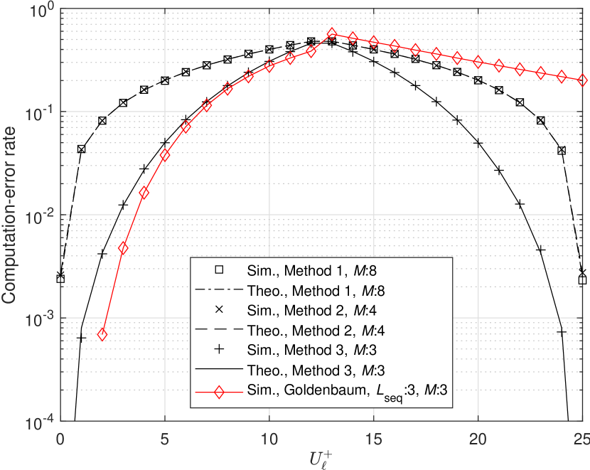
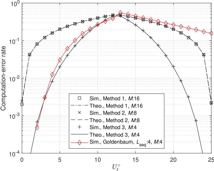
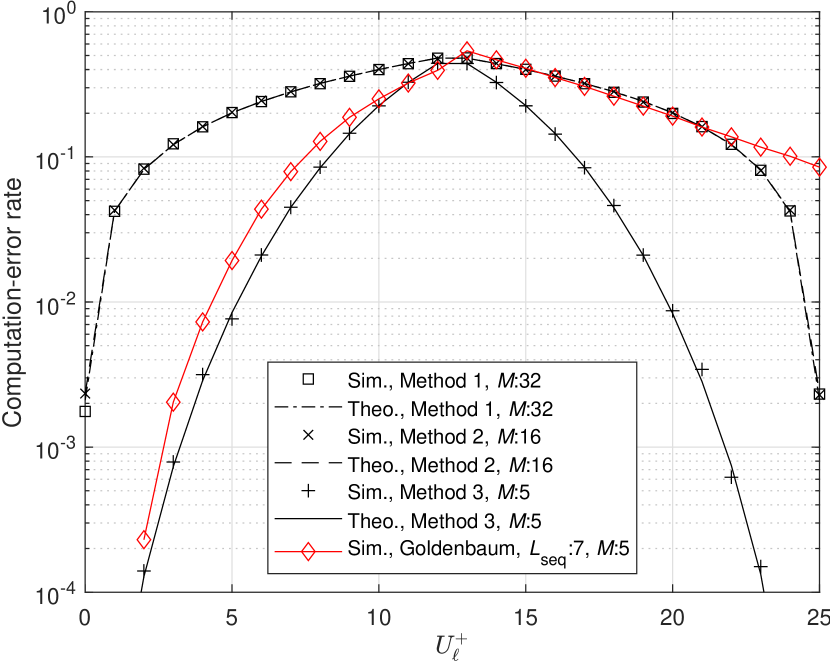
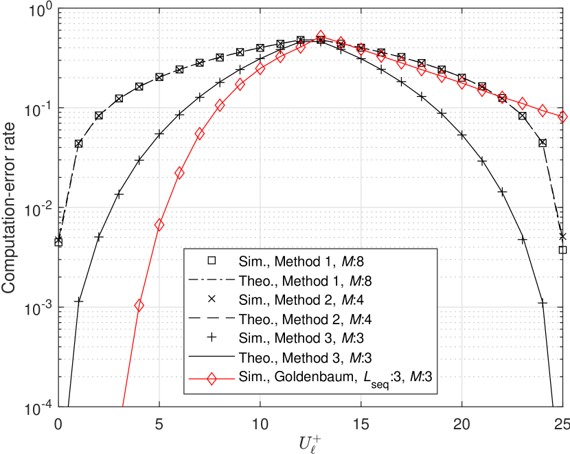
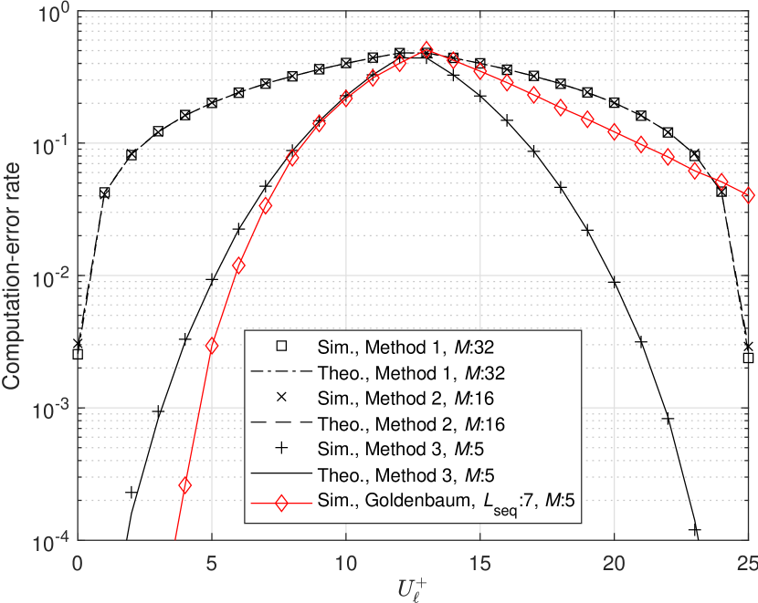
In Figure 3, we demonstrate the CER performance of the schemes for a given number $U^{+}_{\ell}$ for $U=25$ transmitters, ${\tt{SNR}}=10$ dB, and $K\in\{8,16,32\}$. In Figure 3LABEL:sub@subfig:CERL1K8-LABEL:sub@subfig:CERL1K32, we consider flat-fading Rayleigh channel, i.e., $L=1$ tap. As can be seen from the results, increasing $|U^{+}_{\ell}-U^{-}_{\ell}|$ leads to a better CER for all methods. This is expected because the distance between two test values for the proposed methods with a DiZeT decoder increases with $|U^{+}_{\ell}-U^{-}_{\ell}|$. The performance of Method 1 and Method 2 are identical in Figure 3LABEL:sub@subfig:CERL1K8-LABEL:sub@subfig:CERL1K32 as we use the normalization factors in (15) and (16) for Method 1. However, Method 2 does not need a normalization factor, as seen in (22). Compared to Methods 1-2, Method 3 exploits redundancy and results in a remarkably better CER, and the CER improves further for increasing $K$ at the expense of a reduced computation rate. For Goldenbaum’s scheme, the transmitters do not transmit when the devices vote for $-1$, and the impact of the channel on the signal decreases for a smaller $U^{+}_{\ell}$. Thus, Goldenbaum’s scheme causes an asymmetric behavior in CER in the range of $U^{+}_{\ell}$, and the CER degrades considerably by increasing for a large $U^{+}_{\ell}$. In Figure 3LABEL:sub@subfig:CERL5K8-LABEL:sub@subfig:CERL5K32, we assess the CER for a frequency-selective channel with $L=5$ taps and $\rho=1$. Compared to the results in Figure 3LABEL:sub@subfig:CERL1K8-LABEL:sub@subfig:CERL1K32, the CER slightly increases in the selective channel for all proposed methods, while it decreases for Goldenbaum’s scheme. Nonetheless, it is still notable that a low-complexity DiZeT-based detector allows the receiver to compute the MVs without knowing the instantaneous CSI at the transmitters and receiver (i.e., without phase and time synchronization across the devices). Finally, the theoretical CER results based on Corollaries 3-5 are well-aligned with the simulation results in Figure 3.

Refer to caption
Figure 4: PMEPR distribution with DFT-s-OFDM. For OFDM, the PMEPRs of transmitted signals are 1.54 dB and 1.79 dB for $K=32$ and $K=8$, respectively (not shown in the figure as all the sequences lead to an identical PMEPR as Huffman sequences have an identical AACF for a given $K$).

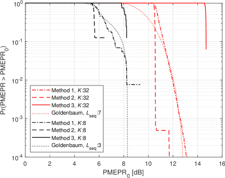
In Figure 4, we analyze the PMEPR distribution of the transmitted signals for $K\in\{8,32\}$. For this analysis, we consider DFT-s-OFDM, i.e., a variant of single-carrier waveform maintaining the linear convolution operation in (1) with zero-padding [15, 37]. We set the DFT and inverse discrete Fourier transform (IDFT) sizes to $K+1$ and $16\times(K+1)$, respectively, to over-sample the signal in the time domain by a factor of $16$. The results in Figure 4 show that the instantaneous power of the transmitted signals can be high and Method 3 causes a higher PMEPR than Methods 1-2. The PMEPR distribution for Goldenbaum’s scheme is also similar to Method 2. It is worth noting that the PMEPR distribution of a single-carrier waveform depends on the distribution of the transmitted symbols. For the proposed methods, the elements of sequences originate from Huffman sequences. The magnitude of one of the sequence elements can be higher than that of the other elements in the sequence, leading to a high instantaneous signal power. If the coherence bandwidth is less than the bandwidth of the channel, i.e., $L=1$, instead of DFT-s-OFDM, a typical orthogonal frequency division multiplexing (OFDM) transmission can also be used for the proposed methods. In this case, the PMEPR of transmitted signals are fixed at 1.54 dB and 1.79 dB for $K=32$, and $K=8$, respectively. This result is expected as Huffman sequences have an identical AACF for a given $K$. Also, OFDM results in low PMEPR for sequences with good autocorrelation properties [40, 41, 42], and the AACF of a Huffman sequence is almost an impulse function.

Refer to caption
Figure 5: The number resources consumed per MV computation for a given number of transmitters ($L=1$).

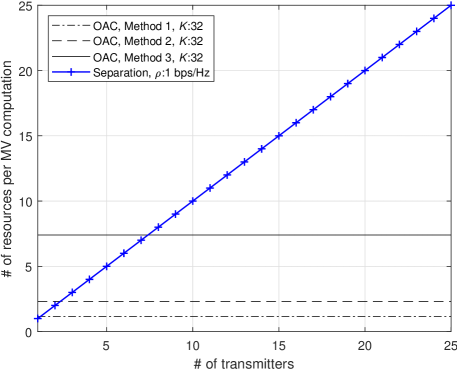
In Figure5, we compare Methods 1-3 with the case where the receiver computes the MV after it acquires each vote over orthogonal resources (i.e., separation of computation and communication) in terms of resource utilization. For the separation, we assume that the spectral efficiency is $\rho=1$ bps/Hz. Since a vote can be represented with a single bit, we can compute the number of resources needed per MV computation as $U/\rho$ resources. Based on the computation rates discussed in Section III, the number of resources per MV are $(K+L)/K$, $(K+L)/(K/2)$, and $(K+L)/(\log_{2}(K)$ for Methods 1-3, respectively. In Figure5, we plot the number of resources consumed per MV computation for a given number of transmitters $U$ for $K=32$ zeros and $L=5$ taps. For Methods 1-3, the number of resources needed per MV can be calculated as $1.2$, $2.3$, and $7.4$ resources/MV, while it linearly increases with the number of transmitters for the separation. Method 3 becomes more efficient than the separation when at least $U=8$ devices are in the network.

Next, we evaluate the schemes for a distributed median computation scenario. For this application, let $s_{\ell,u}$ denote the $\ell$th parameter at the $u$th device, and the goal is to compute the median value of the elements in $\{s_{\ell,1},\hbox to10.00002pt{.\hss.\hss.},s_{\ell,U}\}$ in a distributed manner, $\forall\ell\in\{0,1,\hbox to10.00002pt{.\hss.\hss.},M-1\}$. To this end, let us express the median as a point minimizing the sum of distances to the parameters at the devices as

$\displaystyle c_{\ell}\triangleq\arg\min_{c}L_{\ell}(c)~{},$ (38)

where $c_{\ell}$ is the median value and $L_{\ell}(c)=\sum_{u=1}^{U}\lVert c-s_{\ell,u}\rVert_{2}$ is the corresponding loss function. Since $L_{\ell}(c)$ is convex, (38) can be solved iteratively as

$\displaystyle\hat{c}_{\ell}^{(i+1)}=$ $\displaystyle\hat{c}_{\ell}^{(i)}-\mu^{(i)}\frac{dL_{\ell}(c)}{dc}\bigg{|}_{c=\hat{c}_{\ell}^{(i)}}$
$\displaystyle=$ $\displaystyle\hat{c}_{\ell}^{(i)}-\mu^{(i)}\sum_{u=1}^{U}\text{sign}\left(\hat{c}_{\ell}^{(i)}-s_{\ell,u}\right)~{},$ (39)

where $\hat{c}_{\ell}^{(i)}$ is an estimate of $c_{\ell}$ and $\mu^{(i)}$ is the learning rate at the $i$th iteration. Since the gradient direction can also be used for solving (38) with an accuracy of $\pm\mu^{(i)}$, (39) can be modified as

$\displaystyle\hat{c}_{\ell}^{(i+1)}=\hat{c}_{\ell}^{(i)}-\mu^{(i)}\text{sign}\left(\sum_{u=1}^{U}\text{sign}\left(\hat{c}_{\ell}^{(i)}-s_{\ell,u}\right)\right)~{},$ (40)

where the update in (40) is well-aligned with the MV computation problem in (8). In the case of a distributed scenario, the devices do not share their parameters in the network to promote privacy. Instead, the $u$th device sets the $\ell$th vote as $v^{(u)}_{\ell}=\text{sign}\left(\hat{c}_{\ell}^{(i)}-s_{\ell,u}\right)$ for the $\ell$th parameter at the $i$th iteration, and all devices access the spectrum concurrently for OAC. After the receiver computes the $\ell$th MV with OAC and updates $\hat{c}_{\ell}^{(i)}$ as in (40), it shares $\hat{c}_{\ell}^{(i+1)}$ in the downlink for the next iteration.

Refer to caption
(a) $L=1$ and $K=8$.
Refer to caption
(b) $L=1$ and $K=32$.
Refer to caption
(c) $L=1$ and $K=128$.
Refer to caption
(d) $L=5$, $\rho=1$, and $K=8$.
Refer to caption
(e) $L=5$, $\rho=1$, and $K=32$.
Refer to caption
(f) $L=5$, $\rho=1$, and $K=128$.
Figure 6: RMSE for different number of roots and channel length ($U=25$ transmitters, ${\tt{SNR}}=10$ dB).

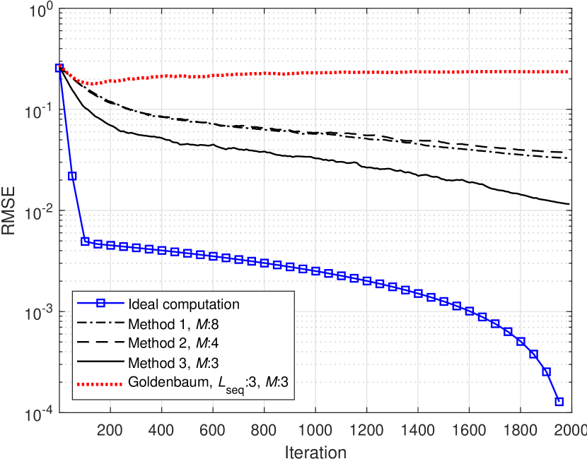
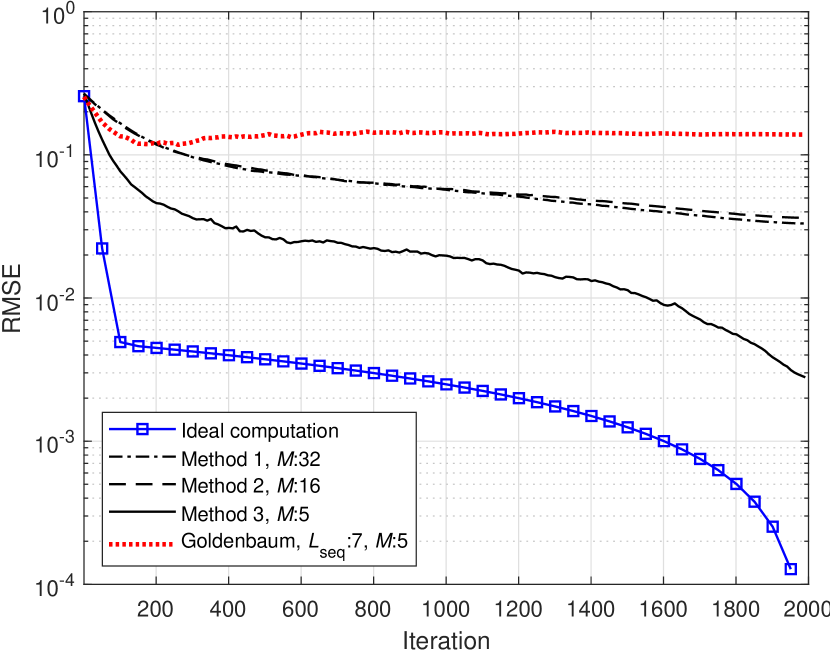
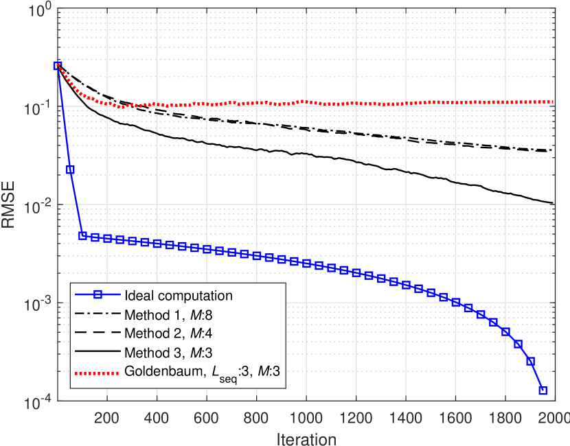
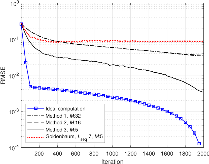
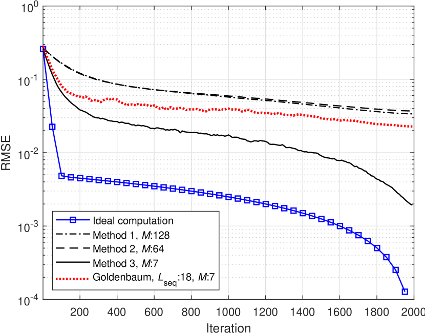
In Figure 6, we plot the root-mean-squared error (RMSE) of $\hat{c}_{\ell}^{(i)}$, i.e., the square root of the arithmetic mean of $|{\hat{c}_{\ell}^{(i)}-c_{\ell}}|^{2}$, over the communication rounds for $K\in\{8,32,128\}$. We consider $U=25$ devices and assume that $s_{\ell,u}\sim{\mathcal{U}_{[-\sqrt{3},\sqrt{3}]}}$, $\forall u$, and reduce $\mu^{(i)}$ from 0.01 to 1e-5 linearly over the iterations. We also generate results when the MV computation occurs without impairments to provide a reference curve. In Figure 6LABEL:sub@subfig:MSEL1K8-LABEL:sub@subfig:MSEL1K128 and Figure 6LABEL:sub@subfig:MSEL5K8-LABEL:sub@subfig:MSEL5K128, we consider flat and frequency-selective fading channels, respectively. Similar to the CER results in Figure 3, Method 3 is superior to Methods 1 and 2, while the performance of Method 1 and Method 2 are almost identical. Increasing the number of roots $K$ also improves the performance of Method 3. For instance, the RMSE reduces to 0.002 for $K=128$ from $0.01$ for $K=8$. Also, the impact of the multipath channel on the RMSE results is negligibly small for the proposed methods. Goldenbaum’s scheme performs worse than Method 3 in the flat-fading channel. However, its performance improves in more selective channels. A larger sequence length $L_{\rm seq}$ leads to a better result, as seen Figure 3LABEL:sub@subfig:MSEL1K128. This is because Goldenbaum’s method is inherently sensitive to the cross-correlation of the sequences used at the transmitters, and the interference due to the cross-products decreases on average for larger sequence lengths. We observe a large gap between the ideal MV computation scenario and all methods based on OAC. Nonetheless, the OAC does not reveal the votes explicitly to the receiver due to the signal superposition while utilizing the spectrum efficiently through simultaneous transmissions on the same resources. In addition, the proposed OAC methods do not use the CSI at the receiver or transmitters, i.e., reducing the potential overheads.

VI Concluding Remarks

In this work, we introduce a new strategy to compute the MV function over the air and discuss three different methods. Fundamentally, the proposed methods rely on nullifying a transmitter’s contribution to the superposed value by encoding the votes, i.e., $+1$ and $-1$, into the zeros of a Huffman polynomial. We prove that this strategy non-coherently superposes the votes on two different test values in the fading channel, and a DiZeT decoder can be used for MV computation. The proposed methods inherently result in a trade-off between the computation rate, CER, and applicability. Method 1 has the highest computation rate. However, the decoder needs the PDP of the channel apriori. Method 2 improves Method 1’s applicability to practice as the decoder does not require the PDP information by using a differential encoder. Method 3 is superior to Method 2 regarding CER, but the computation rate is reduced further. We analyze the CER theoretically for all methods and provide analytical expressions that match the simulation results well. Finally, we show that the proposed methods can be applied to a distributed median computation scenario based on MV computation.

The proposed methods potentially lead to several interesting research directions. For instance, in this work, we choose the radii of roots to maximize the minimum distance between zeros as in [11, 12, 15]. Also, we use two different radii for the roots based on Huffman polynomials. Hence, an unanswered challenge in this work is optimizing the number of radii and their radii for OAC. Secondly, in this work, we consider MV computation. How can we improve the methods for other nomographic functions? In this direction, the representation of integers in binary or balanced systems, as in [29], may be explored. As we demonstrated, the PMEPR of the Huffman sequences for a single-carrier waveform can be high. Hence, another direction is reducing the PMEPR of the transmitted signals for the single-carrier waveform. Finally, assessing the performance of the proposed methods for training a neural network with federated learning is another angle that can be pursued.

Appendix A Proof of Lemma 1

Proof of Lemma 1.

We can express the right-hand side of (12) as

$\displaystyle\mathbb{E}\left[\left|{{S}(d{\rm e}^{\frac{{\rm j}2\pi\ell}{K}})}\right|^{2}\right]$
$\displaystyle\stackrel{{\scriptstyle(a)}}{{=}}\sum_{u=1}^{U}\mathbb{E}\left[|{{H^{(u)}}(d{\rm e}^{\frac{{\rm j}2\pi\ell}{K}})}|^{2}\right]\mathbb{E}\left[|{{X^{(u)}}(d{\rm e}^{\frac{{\rm j}2\pi\ell}{K}})}|^{2}\right]$
$\displaystyle\stackrel{{\scriptstyle(b)}}{{=}}\sum_{\begin{subarray}{c}u=1\\ v^{(u)}_{\ell}=1\end{subarray}}^{U}\mathbb{E}\left[|{{H^{(u)}}(d{\rm e}^{\frac{{\rm j}2\pi\ell}{K}})}|^{2}\right]\mathbb{E}\left[|{{X^{(u)}}(d{\rm e}^{\frac{{\rm j}2\pi\ell}{K}})}|^{2}\right]~{},$ (41)

where (a) is because the channels and transmitted signals are independent random variables and (b) is because ${X^{(u)}}(d{\rm e}^{\frac{{\rm j}2\pi\ell}{K}})=0$ for any $u$ with $v^{(u)}_{\ell}=-1$. By using (7),

$\displaystyle\mathbb{E}\left[|{{X^{(u)}}(d{\rm e}^{\frac{{\rm j}2\pi\ell}{K}})}|^{2}\right]=\mathbb{E}\left[\Big{|}{{x}^{(u)}_{K}\prod_{k=0}^{K-1}\left(d{\rm e}^{\frac{{\rm j}2\pi\ell}{K}}-\alpha^{(u)}_{k}\right)}\Big{|}^{2}\right]$
$\displaystyle~{}~{}~{}~{}~{}~{}~{}~{}~{}~{}~{}~{}~{}=\eta({K+1})\mathbb{E}\left[\prod_{k=0}^{K-1}\frac{\Big{|}d{\rm e}^{\frac{{\rm j}2\pi\ell}{K}}-\alpha^{(u)}_{k}\Big{|}^{2}}{|\alpha^{(u)}_{k}|}\right]~{}.$ (42)

For any $u$ with $v^{(u)}_{\ell}=1$, we can calculate

$\displaystyle\mathbb{E}\left[|{X^{(u)}}(d{\rm e}^{\frac{{\rm j}2\pi\ell}{K}})|^{2}|v^{(u)}_{\ell}=1\right]$
$\displaystyle=\eta({K+1})\frac{(d-d^{-1})^{2}}{d^{-1}}\prod_{\begin{subarray}{c}k=0\\ k\neq\ell\end{subarray}}^{K-1}\mathbb{E}\left[\frac{|d{\rm e}^{\frac{{\rm j}2\pi\ell}{K}}-\alpha^{(u)}_{k}|^{2}}{|\alpha^{(u)}_{k}|}\right]$
$\displaystyle=\eta({K+1})\frac{(d-d^{-1})^{2}}{d^{-1}}$
$\displaystyle~{}~{}~{}~{}\times\prod_{\begin{subarray}{c}k=1\end{subarray}}^{K-1}{\frac{|d-d{\rm e}^{\frac{{\rm j}2\pi k}{K}}|^{2}}{d}}\frac{1}{2}+{\frac{|d-d^{-1}{\rm e}^{\frac{{\rm j}2\pi k}{K}}|^{2}}{d^{-1}}}\frac{1}{2}$
$\displaystyle=\eta({K+1})(d-d^{-1})^{2}d^{{K}}$
$\displaystyle~{}~{}~{}~{}~{}~{}~{}\times\frac{1}{2^{K-1}}\prod_{\begin{subarray}{c}k=1\end{subarray}}^{K-1}{{|1-{\rm e}^{\frac{{\rm j}2\pi k}{K}}|^{2}}+{|d-d^{-1}{\rm e}^{\frac{{\rm j}2\pi k}{K}}|^{2}}}~{}.$ (43)

By plugging (9) and (43) in (41), we obtain (12). ∎

Appendix B Proof of Lemma 2

Proof of Lemma 2.

By using the same arguments for (41), we can express the right-hand side of (18) as

$\displaystyle\mathbb{E}\left[\left|{{S}(d{\rm e}^{\frac{{\rm j}2\pi 2\ell}{K}})}\right|^{2}\right]$
$\displaystyle=\sum_{\begin{subarray}{c}u=1\\ v^{(u)}_{\ell}=1\end{subarray}}^{U}\mathbb{E}\left[|{{H^{(u)}}(d{\rm e}^{\frac{{\rm j}2\pi 2\ell}{K}})}|^{2}\right]\mathbb{E}\left[|{{X^{(u)}}(d{\rm e}^{\frac{{\rm j}2\pi 2\ell}{K}})}|^{2}\right]~{}.$ (44)

By using (42), for any $u$ with $v^{(u)}_{\ell}=1$, we can calculate

$\displaystyle\mathbb{E}\left[|{X^{(u)}}(d{\rm e}^{\frac{{\rm j}2\pi 2\ell}{K}})|^{2}|v^{(u)}_{\ell}=1\right]$
$\displaystyle=\eta({K+1})\frac{(d-d^{-1})^{2}}{d^{-1}}\frac{|d-d{\rm e}^{\frac{2\pi}{K}}|^{2}}{d}$
$\displaystyle~{}~{}~{}~{}~{}~{}~{}~{}~{}~{}~{}\times\prod_{\begin{subarray}{c}k=0\\ k\neq\ell\end{subarray}}^{\frac{K}{2}-1}\mathbb{E}\left[\frac{|d{\rm e}^{\frac{{\rm j}2\pi\ell}{K}}-\alpha^{(u)}_{2k}|^{2}}{|\alpha^{(u)}_{2k}|}\frac{|d{\rm e}^{\frac{{\rm j}2\pi\ell}{K}}-\alpha^{(u)}_{2k+1}|^{2}}{|\alpha^{(u)}_{2k+1}|}\right]$
$\displaystyle=\eta({K+1})\frac{(d-d^{-1})^{2}}{d^{-1}}\frac{|d-d{\rm e}^{\frac{2\pi}{K}}|^{2}}{d}$
$\displaystyle~{}~{}~{}~{}~{}~{}~{}~{}~{}~{}~{}~{}~{}~{}\times\prod_{\begin{subarray}{c}k=1\end{subarray}}^{\frac{K}{2}-1}{\frac{|d-d{\rm e}^{\frac{{\rm j}2\pi 2k}{K}}|^{2}}{d}}{\frac{|d-d^{-1}{\rm e}^{\frac{{\rm j}2\pi(2k+1)}{K}}|^{2}}{d^{-1}}}\frac{1}{2}$
$\displaystyle~{}~{}~{}~{}~{}~{}~{}~{}~{}~{}~{}~{}~{}~{}~{}~{}~{}~{}~{}~{}+{\frac{|d-d^{-1}{\rm e}^{\frac{{\rm j}2\pi 2k}{K}}|^{2}}{d}}{\frac{|d-d{\rm e}^{\frac{{\rm j}2\pi(2k+1)}{K}}|^{2}}{d^{-1}}}\frac{1}{2}$
$\displaystyle=\eta({K+1})(d-d^{-1})^{2}|1-{\rm e}^{\frac{2\pi}{K}}|^{2}d^{K}$
$\displaystyle~{}~{}~{}~{}~{}~{}\times\frac{1}{2^{\frac{K}{2}-1}}\prod_{\begin{subarray}{c}k=1\end{subarray}}^{\frac{K}{2}-1}{{|1-{\rm e}^{\frac{{\rm j}2\pi 2k}{K}}|^{2}}}{{|d-d^{-1}{\rm e}^{\frac{{\rm j}2\pi(2k+1)}{K}}|^{2}}}$
$\displaystyle~{}~{}~{}~{}~{}~{}~{}~{}~{}~{}~{}~{}~{}~{}~{}~{}~{}~{}~{}~{}+{|1-{\rm e}^{\frac{{\rm j}2\pi(2k+1)}{K}}|^{2}}{{|d-d^{-1}{\rm e}^{\frac{{\rm j}2\pi 2k}{K}}|^{2}}}~{}.$ (45)

By plugging (9) and (45) in (44), we obtain (18). ∎

Appendix C Proof of Lemma 3

Proof of Lemma 3.

We can express the right-hand side of (24) as

$\displaystyle\mathbb{E}\left[\left|{{S}(d{\rm e}^{\frac{{\rm j}2\pi l}{K}})}\right|^{2}\right]$
$\displaystyle=\sum_{\begin{subarray}{c}u=1\\ \sum_{\ell=0}^{M-1}b^{(u)}_{\ell}2^{\ell}=l\end{subarray}}^{U}\mathbb{E}\left[|{{H^{(u)}}(d{\rm e}^{\frac{{\rm j}2\pi l}{K}})}|^{2}\right]\mathbb{E}\left[|{{X^{(u)}}(d{\rm e}^{\frac{{\rm j}2\pi l}{K}})}|^{2}\right]$
$\displaystyle=\frac{U^{+}_{\ell}\mathbb{I}\left[{l_{\ell}=1}\right]+U^{-}_{\ell}\mathbb{I}\left[{l_{\ell}=0}\right]}{2^{\log_{2}({K})-1}}\mathbb{E}\left[|{{H^{(u)}}(d{\rm e}^{\frac{{\rm j}2\pi l}{K}})}|^{2}\right]$
$\displaystyle~{}~{}~{}~{}~{}~{}~{}~{}~{}~{}~{}~{}~{}~{}~{}~{}~{}\times\mathbb{E}\left[|{{X^{(u)}}(d{\rm e}^{\frac{{\rm j}2\pi l}{K}})|^{2}|\sum_{\ell=0}^{M-1}b^{(u)}_{\ell}2^{\ell}=l}\right]~{}.$ (46)

By using (42), we can calculate

$\displaystyle\mathbb{E}\left[|{{X^{(u)}}(d{\rm e}^{\frac{{\rm j}2\pi l}{K}})|^{2}|\sum_{\ell=0}^{M-1}b^{(u)}_{\ell}2^{\ell}=l}\right]$
$\displaystyle=\eta({K+1})\frac{|d{\rm e}^{\frac{{\rm j}2\pi l}{K}}-d^{-1}{\rm e}^{\frac{{\rm j}2\pi l}{K}}|^{2}}{d^{-1}{\rm e}^{\frac{{\rm j}2\pi l}{K}}}\prod_{\begin{subarray}{c}k=0\\ k\neq\ell\end{subarray}}^{K-1}{\frac{|d{\rm e}^{\frac{{\rm j}2\pi l}{K}}-d{\rm e}^{\frac{{\rm j}2\pi k}{K}}|^{2}}{|d{\rm e}^{\frac{{\rm j}2\pi k}{K}}|}}$
$\displaystyle=\eta({K+1})(d-d^{-1})^{2}d^{K}\prod_{\begin{subarray}{c}k=1\end{subarray}}^{K-1}{{|1-{\rm e}^{\frac{{\rm j}2\pi k}{K}}|^{2}}}$
$\displaystyle=\eta({K+1})(d-d^{-1})^{2}d^{K}K^{2}~{}.$ (47)

By plugging (9) and (47) in (46), we obtain (24). ∎

Appendix D From zeros to polynomial coefficients

Consider the polynomial given in (5). Let us define $y_{p}^{(u)}$ as

$\displaystyle y_{p}^{(u)}\triangleq{X^{(u)}}(z)|_{z={\rm e}^{{\rm j}2\pi\frac{p}{K+1}}}.$ (48)

for $p\in\{0,1,\hbox to10.00002pt{.\hss.\hss.},K\}$. Thus,

$\displaystyle y_{p}^{(u)}=\sum_{n=0}^{K}{x}^{(u)}_{n}{\rm e}^{{\rm j}2\pi\frac{pn}{K+1}}={x}^{(u)}_{K}\prod_{k=0}^{K-1}({\rm e}^{{\rm j}2\pi\frac{p}{K+1}}-\alpha^{(u)}_{k})~{}.$ (49)

The left-hand side of (49) corresponds to $(K+1)$-point IDFT of the sequence $\textit{{x}}^{(u)}=({x}^{(u)}_{0},{x}^{(u)}_{1},\dots,{x}^{(u)}_{K})$. Hence, to obtain $\textit{{x}}^{(u)}$ from the zeros, we apply the $(K+1)$-point DFT to the right-hand side of (49) as

$\displaystyle{x}^{(u)}_{n}$ $\displaystyle=\frac{1}{K+1}\sum_{p=0}^{K}y_{p}^{(u)}{\rm e}^{-{\rm j}2\pi\frac{pn}{K+1}}$
$\displaystyle=\frac{{x}^{(u)}_{K}}{K+1}\sum_{p=0}^{K}{\rm e}^{-{\rm j}2\pi\frac{pn}{K+1}}\prod_{k=0}^{K-1}({\rm e}^{{\rm j}2\pi\frac{p}{K+1}}-\alpha^{(u)}_{k})$ (50)

for $n\in\{0,1,\hbox to10.00002pt{.\hss.\hss.},K\}$.

Appendix E Proofs of Corollary (3) and Corollary (4)

Proof of Corollary (3).

By using (15) and (16), we obtain

$\displaystyle\mathrm{Pr}({{\tilde{U}^{+}_{\ell}-\tilde{U}^{-}_{\ell}<0};\textit{{{V}}}})$
$\displaystyle~{}~{}~{}~{}~{}~{}=\mathrm{Pr}({\frac{\left|{{R}(d{\rm e}^{\frac{{\rm j}2\pi\ell}{K}})}\right|^{2}}{\mathcal{X}_{1}(d)\Gamma(d)}-\frac{\left|{{R}(d^{-1}{\rm e}^{\frac{{\rm j}2\pi\ell}{K}})}\right|^{2}}{\mathcal{X}_{1}(d^{-1})\Gamma(d^{-1})}<x;\textit{{{V}}}})$

for $x={{\Omega}(d)}/({\mathcal{X}_{1}(d)\Gamma(d)})-{{\Omega}(d^{-1})}/({\mathcal{X}_{1}(d^{-1})\Gamma(d^{-1})})$. For a given a set of votes, $|{{R}(d{\rm e}^{\frac{{\rm j}2\pi l}{K}})}|^{2}/(\mathcal{X}_{1}(d)\Gamma(d))$ is an exponential random variable with the mean $\lambda_{+}^{-1}$ because ${H^{(u)}}(d{\rm e}^{\frac{{\rm j}2\pi l}{K}})$, $\forall u$, and ${W}(d{\rm e}^{\frac{{\rm j}2\pi l}{K}})$ are independent random variables following zero-mean symmetric complex Gaussian distribution. A similar deduction can be made for $|{{R}(d^{-1}{\rm e}^{\frac{{\rm j}2\pi l}{K}})}|^{2}/(\mathcal{X}_{1}(d^{-1})\Gamma(d^{-1}))$, leading to $\lambda_{-}^{-1}$. ∎

Proof of Corollary (4).

For a given a set of votes, $|{{R}(d{\rm e}^{\frac{{\rm j}2\pi l}{K}})}|^{2}$ is an exponential random variable where its mean is $\lambda_{l}^{-1}=\Gamma(d)\sum_{u=1}^{U}|{X^{(u)}}(d{\rm e}^{\frac{{\rm j}2\pi l}{K}})|^{2}+{\Omega}(d)$ because ${H^{(u)}}(d{\rm e}^{\frac{{\rm j}2\pi l}{K}})$, $\forall u$, and ${W}(d{\rm e}^{\frac{{\rm j}2\pi l}{K}})$ are independent random variables following zero-mean symmetric complex Gaussian distribution. ∎

References

  • [1] A. Şahin, “Majority vote computation with modulation on conjugate-reciprocal zeros,” in Proc. IEEE Global Communications Conference (GLOBECOM), Dec. 2024, pp. 1–6 (under review).
  • [2] B. Nazer and M. Gastpar, “Computation over multiple-access channels,” IEEE Trans. Inf. Theory, vol. 53, no. 10, pp. 3498–3516, Oct. 2007.
  • [3] M. Goldenbaum, H. Boche, and S. Stańczak, “Harnessing interference for analog function computation in wireless sensor networks,” IEEE Trans. Signal Process., vol. 61, no. 20, pp. 4893–4906, 2013.
  • [4] ——, “Nomographic functions: Efficient computation in clustered Gaussian sensor networks,” IEEE Trans. Wireless Commun., vol. 14, no. 4, pp. 2093–2105, 2015.
  • [5] U. Altun, G. Karabulut Kurt, and E. Ozdemir, “The magic of superposition: A survey on simultaneous transmission based wireless systems,” IEEE Access, vol. 10, pp. 79 760–79 794, 2022.
  • [6] A. Şahin and R. Yang, “A survey on over-the-air computation,” IEEE Commun. Surveys Tuts., vol. 25, no. 3, pp. 1877–1908, Apr. 2023.
  • [7] Z. Chen, E. G. Larsson, C. Fischione, M. Johansson, and Y. Malitsky, “Over-the-air computation for distributed systems: Something old and something new,” IEEE Network, pp. 1–7, 2023.
  • [8] H. Hellström, J. M. B. da Silva Jr., M. M. Amiri, M. Chen, V. Fodor, H. V. Poor, and C. Fischione, “Wireless for machine learning: A survey,” Foundations and Trends in Signal Processing, vol. 15, no. 4, pp. 290–399, 2022.
  • [9] Z. Wang, Y. Zhao, Y. Zhou, Y. Shi, C. Jiang, and K. B. Letaief, “Over-the-air computation: Foundations, technologies, and applications,” 2022. [Online]. Available: https://arxiv.org/abs/2210.10524
  • [10] P. Walk, P. Jung, and B. Hassibi, “Short-message communication and FIR system identification using Huffman sequences,” in Proc. IEEE International Symposium on Information Theory (ISIT), 2017, pp. 968–972.
  • [11] ——, “MOCZ for blind short-packet communication: Basic principles,” IEEE Trans. Wireless Commun., vol. 18, no. 11, pp. 5080–5097, 2019.
  • [12] P. Walk, P. Jung, B. Hassibi, and H. Jafarkhani, “MOCZ for blind short-packet communication: Practical aspects,” IEEE Trans. Wireless Commun., vol. 19, no. 10, pp. 6675–6692, 2020.
  • [13] J. H. Wilkinson, “The perfidious polynomial,” Studies in Numerical Analysis, vol. 24, pp. 1–28, 1984.
  • [14] D. Huffman, “The generation of impulse-equivalent pulse trains,” IRE Transactions on Information Theory, vol. 8, no. 5, pp. 10–16, 1962.
  • [15] P. Walk and W. Xiao, “Multi-user MOCZ for mobile machine type communications,” in Proc. IEEE Wireless Communications and Networking Conference (WCNC), 2021, pp. 1–6.
  • [16] S. K. Dehkordi, P. Jung, P. Walk, D. Wieruch, K. Heuermann, and G. Caire, “Integrated sensing and communication with MOCZ waveform,” 2023.
  • [17] Y. Sun, Y. Zhang, G. Dou, Y. Lu, and Y. Song, “Noncoherent SIMO transmission via MOCZ for short packet-based machine-type communications in frequency-selective fading environments,” IEEE Open Journal of the Communications Society, vol. 4, pp. 1544–1550, 2023.
  • [18] A. A. Siddiqui, E. Bedeer, H. H. Nguyen, and R. Barton, “Spectrally-efficient modulation on conjugate-reciprocal zeros (se-mocz) for non-coherent short packet communications,” IEEE Transactions on Wireless Communications, vol. 23, no. 3, pp. 2226–2240, 2024.
  • [19] M. M. Amiri and D. Gündüz, “Federated learning over wireless fading channels,” IEEE Trans. Wireless Commun., vol. 19, no. 5, pp. 3546–3557, Feb. 2020.
  • [20] G. Zhu, Y. Wang, and K. Huang, “Broadband analog aggregation for low-latency federated edge learning,” IEEE Trans. Wireless Commun., vol. 19, no. 1, pp. 491–506, Jan. 2020.
  • [21] G. Zhu, Y. Du, D. Gündüz, and K. Huang, “One-bit over-the-air aggregation for communication-efficient federated edge learning: Design and convergence analysis,” IEEE Trans. Wireless Commun., vol. 20, no. 3, pp. 2120–2135, Nov. 2021.
  • [22] W. Guo, R. Li, C. Huang, X. Qin, K. Shen, and W. Zhang, “Joint device selection and power control for wireless federated learning,” IEEE J. Sel. Areas Commun., vol. 40, no. 8, pp. 2395–2410, 2022.
  • [23] A. Şahin, “A demonstration of over-the-air computation for federated edge learning,” in IEEE Globecom Workshops (GC Wkshps), 2022, pp. 1821–1827.
  • [24] H. Jung and S.-W. Ko, “Performance analysis of UAV-enabled over-the-air computation under imperfect channel estimation,” IEEE Wireless Commun. Lett., pp. 1–1, Nov. 2021.
  • [25] G. Mergen and L. Tong, “Type based estimation over multiaccess channels,” IEEE Trans. Signal Process., vol. 54, no. 2, pp. 613–626, 2006.
  • [26] G. Mergen, V. Naware, and L. Tong, “Asymptotic detection performance of type-based multiple access over multiaccess fading channels,” IEEE Trans. Signal Process., vol. 55, no. 3, pp. 1081–1092, 2007.
  • [27] A. Şahin, “Distributed learning over a wireless network with non-coherent majority vote computation,” IEEE Trans. Wireless Commun., pp. 1–16, 2023.
  • [28] S. S. M. Hoque and A. Şahin, “Chirp-based majority vote computation for federated edge learning and distributed localization,” IEEE Open Journal of the Communications Society, pp. 1–1, 2023.
  • [29] A. Şahin, “Over-the-air computation based on balanced number systems for federated edge learning,” IEEE Trans. Wireless Commun., Oct. 2023.
  • [30] M. Goldenbaum and S. Stanczak, “Robust analog function computation via wireless multiple-access channels,” IEEE Trans. Commun., vol. 61, no. 9, pp. 3863–3877, 2013.
  • [31] ——, “On the channel estimation effort for analog computation over wireless multiple-access channels,” IEEE Wireless Commun. Lett., vol. 3, no. 3, pp. 261–264, 2014.
  • [32] A. Şahin, “A demonstration of over-the-air-computation for FEEL,” in Proc. IEEE Global Communications Conference Workshops (GLOBECOM WRKSHP) - Edge Learning over 5G Mobile Networks and Beyond, Dec. 2022, pp. 1–7.
  • [33] A. Gadre, F. Yi, A. Rowe, B. Iannucci, and S. Kumar, “Quick (and dirty) aggregate queries on low-power WANs,” in Proc. ACM/IEEE International Conference on Information Processing in Sensor Networks (IPSN), 2020, pp. 277–288.
  • [34] A. Kortke, M. Goldenbaum, and S. Stańczak, “Analog computation over the wireless channel: A proof of concept,” in Proc. IEEE Sensors, 2014, pp. 1224–1227.
  • [35] E. Dahlman, S. Parkvall, and J. Skold, 5G NR: The Next Generation Wireless Access Technology, 1st ed.   USA: Academic Press, Inc., 2018.
  • [36] B. Tegin and T. M. Duman, “Federated learning with over-the-air aggregation over time-varying channels,” IEEE Trans. Wireless Commun., pp. 1–14, 2023.
  • [37] A. Sahin, R. Yang, E. Bala, M. C. Beluri, and R. L. Olesen, “Flexible DFT-S-OFDM: Solutions and challenges,” IEEE Communications Magazine, vol. 54, no. 11, pp. 106–112, 2016.
  • [38] A. Şahin and X. Wang, “Reliable majority vote computation with complementary sequences for UAV waypoint flight control,” arXiv preprint arXiv:2309.15193, 2023.
  • [39] L. A. Waller, B. W. Turnbull, and J. M. Hardin, “Obtaining distribution functions by numerical inversion of characteristic functions with applications,” The American Statistician, vol. 49, no. 4, pp. 346–350, 1995.
  • [40] A. Şahin and R. Yang, “A generic complementary sequence construction and associated encoder/decoder design,” IEEE Trans. Commun., pp. 1–15, 2021.
  • [41] J. A. Davis and J. Jedwab, “Peak-to-mean power control in OFDM, Golay complementary sequences, and Reed-Muller codes,” IEEE Trans. Inf. Theory, vol. 45, no. 7, pp. 2397–2417, Nov. 1999.
  • [42] M. Golay, “Complementary series,” IRE Trans. Inf. Theory, vol. 7, no. 2, pp. 82–87, Apr. 1961.