CoverLib: Classifiers-equipped Experience Library by Iterative Problem Distribution Coverage Maximization for Domain-tuned Motion Planning

Abstract

Library-based methods are known to be very effective for fast motion planning by adapting an experience retrieved from a precomputed library. This article presents CoverLib, a principled approach for constructing and utilizing such a library. CoverLib iteratively adds an experience-classifier-pair to the library, where each classifier corresponds to an adaptable region of the experience within the problem space. This iterative process is an active procedure, as it selects the next experience based on its ability to effectively cover the uncovered region. During the query phase, these classifiers are utilized to select an experience that is expected to be adaptable for a given problem. Experimental results demonstrate that CoverLib effectively mitigates the trade-off between plannability and speed observed in global (e.g. sampling-based) and local (e.g. optimization-based) methods. As a result, it achieves both fast planning and high success rates over the problem domain. Moreover, due to its adaptation-algorithm-agnostic nature, CoverLib seamlessly integrates with various adaptation methods, including nonlinear programming-based and sampling-based algorithms.

I Introduction

Motion planning has been studied from two ends of the spectrum: global and local methods. Global methods, such as sampling-based motion planners (SBMP) like Probabilistic Roadmap (PRM) [1] and Rapidly-exploring Random Tree (RRT) [2], are expected to find a solution if one exists, given enough time. However, these methods often require long and varying amount of computational time to obtain even a highly suboptimal solution and are sensitive to the complexity of the problem. On the other hand, local methods, including optimization-based approaches such as CHOMP [3] and TrajOpt [4], as well as SBMP with informed sampling, can quickly find a high-quality solution given a good initial guess, but struggle with problems that are far from the initial guess. There is a trade-off between plannability and speed when comparing global and local methods. In practice, it is often possible to define the scope of the domain, which can be helpful in circumventing this trade-off and enabling quick solutions to a broad range of problems within a specific domain of interest. This is common in many practical robotics applications. For example, in automation for factories or warehouses, the environment and task types are fixed, but the specifics of each task may vary. Similarly, in home service robotics, although the tasks are diverse, the tasks that act as bottlenecks are often known in advance (e.g., reaching into a narrow container).

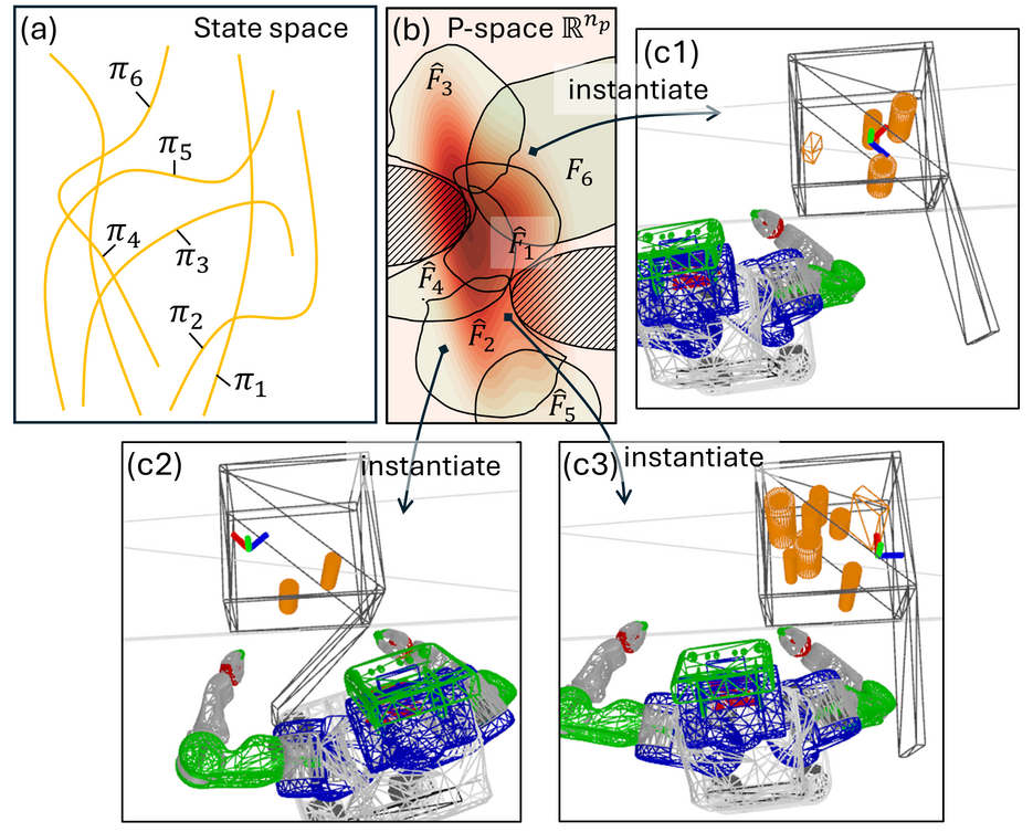
Figure 1: Illustration of CoverLib’s library and the problem (P-) space. (a) The experiences (paths) $\pi_{1:6}$ defined in a state space, e.g. configuration space or phase space. (b) The problem distribution $p(\theta)$ (contour plot) in P-space covered by the union of the estimated adaptable regions $\hat{F}_{1:6}$ (green regions) of the experiences. Note that though depicted in 2D, the P-space is often high-dimensional as it encodes problem settings including obstacle environments, constraints, success condition specifications, etc. (c) Instantiation of three problems from the P-space.

A promising approach to this end is to use a library of experiences[5, 6, 7, 8, 9, 10] reviewed in Section II-A. An experience in this context refers to a previously solved solution path or trajectory, while the library is a collection of such experiences. The key insight is that if two problems are similar, the solution to one can be efficiently adapted to solve the other. Therefore, if the domain of interest is known a priori, the following preprocessing is beneficial: sample a problem, solve it, and store the solution as an experience, repeating this process multiple times. Then, during the online phase, an adaptation algorithm can be used with a retrieved experience from the library to solve new problems quickly.

The library-based approach can be factorized into the high-level and low-level parts. The high-level parts are responsible for the construction and query of the library, while the low-level part is responsible for the internal adaptation algorithm. The high-level parts are adaptation-algorithm-agnostic (treating the adaptation algorithm as an input), allowing the library to be used with any adaptation algorithm, e.g., sampling-based or nonlinear programming- (NLP-) based. Although the low-level part has been extensively studied as reviewed in Section II-A, the high-level counterpart has often received less attention in the community, with the exception of the line of seminal works [11, 12, 13] by Islam et al. reviewed in Section II-B. In fact, most library-based approaches consist of passive library construction and nearest neighbor search, neither of which reflects the domain structure or the characteristics of the adaptation algorithm.

The objective of this paper is to present CoverLib, a principled approach to precomputing libraries tailored to specific domains, which highlights the high-level parts of library-based methods. We define coverage as the proportion of problems that can be solved using the library. CoverLib constructs a library with the explicit aim of maximizing this coverage. CoverLib is designed to iteratively improve the coverage through an active procedure, where the next experience is actively determined to maximize coverage gain. The key component of the algorithm is a set of binary classifiers that identify the adaptable regions for each experience in the library. An adaptable region, roughly speaking, is a region in the problem space (P-space) where the experience is expected to be adaptable. By explicitly tracking the adaptable regions of the experiences added so far, we can actively sample an experience whose adaptable region covers the previously uncovered region effectively, i.e. that has high coverage gain. In the query phase, we utilize the classifiers to determine an experience expected to be adaptable for a given problem. Thus, CoverLib’s library consists of pairs of experience and classifier, as illustrated in Fig. 1.

The active iteration in the library construction process makes CoverLib domain-tuned. This iteration is expected to concentrate experiences on the more challenging parts of the problem distribution and focus on dimensions with greater impact on adaptation, while ignoring those with less impact. Thus, it makes the library less susceptible to the curse of dimensionality. Furthermore, the query phase is also inherently domain-tuned, as the classifiers are trained to explicitly capture each experience’s adaptability.

II Related work and Contributions

II-A Library based motion planning

The adaptation algorithm, the low-level part, of library-based methods has been extensively studied. In NLP-based motion planning, the experienced solution serves as an initializer, and the optimization algorithm acts as the adaptation mechanism. This line of work has been explored using both unconstrained [5] and constrained [6, 7] formulations, and has even been applied to whole-body model predictive control (MPC) [8] using differential dynamic programming. In SBMP, Lightning [9] detects the parts of the experience that are in collision and repairs such parts by generating a new path. Meanwhile, ERT(-Connect) [10] extracts a micro-experience from an experience retrieved from the library and deforms it to generate task-relevant node-transitions.

As for the high-level part, all of the above adopt nearest-neighbour search or some variants for the query part. While most use passive random sampling for the library construction part, others do not mention it. Among them, [6] is the pioneering work that argues for the sample efficiency of nearest neighbour search combined with random sampling-based library construction. The author argued that, under certain settings and with an adaptation strategy, an exponential number of experiences would be needed to achieve adaptation with a bounded optimality gap as the dimensionality of the P-space increases. This analysis relies on the fact, proven that there exists a small ball around each problem parameter, inside which the adaptation of the solution to the problem is guaranteed to be feasible with a bounded optimality gap. A similar conclusion could be drawn for the general nearest-neighbour based library method, with the key point being that the adoption of nearest neighbour search implicitly assumes each experience is homogeneously effective throughout the P-space with a constant distance metric.

However, such a “small ball assumption” is often overly conservative, as suggested by the results and discussion in Sections VI and VII. In reality, adaptable regions are often quite large and irregularly shaped (see Fig. 14), sometimes to the extent that a specific dimension is almost irrelevant for adaptability. This suggests that the adaptation algorithm has a certain nonlinear dimensionality reduction nature. The classifiers in Coverlib’s library are expected to capture this irregularity and dimensionality reduction. Consequently, the number of experiences needed to cover the P-space is expected to be much smaller than the exponential number suggested by the small ball assumption.

II-B Constant-time motion planning by preprocessing

Islam et al. [11] proposed a library-based method that guarantees constant-time (or -iteration) solvability for a finite set of problems created by discretizing the continuous space. They presented a novel preprocessing method that iteratively precomputes an experience and its adaptable set (analogous to an adaptable region) pairs, saving them as a hash table. The iterative algorithm selects the new experience to solve at least one problem not yet covered by the union of the adaptable sets. This process continues until the feasible problem set is completely covered. This method avoids solving the entire problem set in a brute force manner and storing all the solutions. This approach is extended to the case where replanning is required to grasp a moving object [12]. Furthermore, a similar philosophy is found in their recently proposed library based method [13] for a more specific problem setting.

However, these methods are based on discretization, which is inherently prone to the curse of dimensionality. In contrast, Coverlib’s library is expected to be less prone to the curse of dimensionality, as stated in Section II-A.

The adoption of a continuous P-space formulation (in Section III) does not strictly guarantee constant-time adaptability, which is a significant feature of Islam et al.’s methods. However, the proposed method offers a practical approach to this challenge by using Monte Carlo (MC) integration with a large number of samples to effectively validate the classifier’s false-positive rate. To enable this MC integration without prohibitive computational costs, we developed a simple caching mechanism.

While our method shares similarities with Islam et al.’s methods [11, 12] in its iterative library population with awareness of uncovered problems, the continuous-discrete difference leads to three crucial algorithmic distinctions: (a) the use of a classifier, as the adaptable region is no longer enumerable; (b) enforcing the false positive constraint, as the classifier is never perfect; and (c) the active sampling of the next experience explicitly aiming to maximize coverage gain, as in practice only a limited number of iterations are allowed due to the high computational cost of obtaining the classifier.

II-C Other motion planning methods with learning

Learning sampling distributions: Learning sampling distributions is a promising approach to boost the performance of SBMP by focusing samples on relevant regions of the configuration space (C-space). Lehner et al. [14] learn the sampling distribution directly using Gaussian mixture models. Ichter et al. [15] train a conditional variational autoencoder (CVAE) to generate not only domain-conditioned but also problem-conditioned samples. Chamzas et al. [16, 17] demonstrate that learning primitive distributions associated with obstacle pairs is effective.

Learning heuristic maps: When planners have access to importance values (e.g., criticality or domain-relevance), such information can be harnessed in sample or connection generation for SBMPs. Zucker et al. [18] learn a heuristic map of the workspace for fixed environments using reinforcement learning, which is then used for sampling in the C-space by solving inverse kinematics (IK). Terasawa et al. [19] learn a mapping from occupancy grid maps to heuristic values in task space for Task-Space RRT. Ichter et al. [20] propose a deep neural network to learn a mapping from configuration pairs and local geometric features to criticality, which excels for narrow passage problems.

Learning latent spaces: The key insight in this line of research is that there often exists a latent space that is far more simpler than the original C-space. MPNet [21] trains an encoder network modeling a mapping from a C-space to a latent space and a planning network that outputs the next configuration conditioned on obstacle information encoded in the latent space. Ando et al. [22] learn a mapping and its inverse between the C-space and a latent space, ensuring that straight lines in the latent space are collision-free. Ichter et al. [23] take a factorized approach; they train distinct neural networks for forward/inverse-mapping to the latent space, dynamics in the latent space, and collision checking using the latent states.

Learning roadmaps: PRMs may also be considered as a data-driven approach because they precompute a graph in the C-space [1]. Thunder [24], an extension of PRM, adopts a sparse data structure for memory efficiency and lazy collision checking for handling changing environments, outperforming the Lightning method [9] in high-dimensional C-spaces.

II-D Contribution statement

We formulate a domain-tuned library construction problem and propose a practical method (CoverLib) to solve this problem approximately. Unlike the methods based on passive random sampling or nearest neighbor search in Section II-A or discretization in Section II-B, the proposed method is expected to be far less susceptible to the curse of dimensionality, as the classifier can capture the dimensionality reduction nature of the adaptation algorithm, as discussed in Section II-A.

It is important to note that, due to its adaptation-algorithm-agnostic nature, CoverLib is not mutually exclusive with the methods in Section II-C and could be seamlessly integrated with them. In fact, the learned sampling distributions, heuristic maps, and latent spaces can potentially be harnessed to boost the efficiency of the low-level part, the adaptation algorithm.

III Problem formulation for library construction by coverage maximization

Let $\theta\in\mathbb{R}^{n_{p}}$ be a (Problem-) P-parameter which uniquely represents a planning problem and $\mathbb{R}^{n_{p}}$ be a P-space. Note that we may refer to $\theta$ as a “problem”, although it is actually a vector representation of a problem. Let $p(\theta)$ be a distribution of the P-parameter. Let $p(c|\theta,\pi)$ be a distribution of the computational cost $c\in\mathbb{R}$ of an adaptation algorithm when solving a problem $\theta$ using an experience $\pi$. The computational cost is associated with a threshold $c_{\mathrm{max}}\in\mathbb{R}$, and adaptation is considered to fail if $c>c_{\mathrm{max}}$. Let $\hat{f}_{\pi}(\theta)$ be a real-valued estimator for $p(c|\theta,\pi)$. Using this, we define an estimated adaptable region as follows:

$$\hat{F}_{\pi}:=\{\theta:\hat{f}_{\pi}(\theta)\leq c_{\mathrm{max}}\}$$ (1)

where the region is associated with the experience $\pi$. It is important to note that the pair $(\hat{f}_{\pi},c_{\mathrm{max}})$ forms a binary classifier for $c\leq c_{\mathrm{max}}$.

Let $\pi_{1:k}$ be an indexed set of $k$ experiences. Also, for simplicity, let us write $\hat{f}_{i}:=\hat{f}_{\pi_{i}}$ and $\hat{F}_{i}:=\hat{F}_{\pi_{i}}$. The estimated coverage rate $r(\hat{f}_{1:k})$ is defined as follows:

$$r(\hat{f}_{1:k}):=\mathbb{P}_{\theta}\left[\theta\in\cup_{i=1}^{k}\hat{F}_{i}\right]$$ (2)

where $\theta\sim p(\theta)$. Let $i^{*}(\theta)$ be the optimal index selection function that selects the index of the experience minimizing the estimated computational cost for a given problem $\theta$:

$$i^{*}(\theta):=\operatornamewithlimits{argmin}_{i\in\{1..k\}}\hat{f}_{i}(\theta).$$ (3)

The false positive (FP) rate $\alpha(\pi_{1:k},\hat{f}_{1:k})$ is defined as follows:

$$\alpha(\pi_{1:k},\hat{f}_{1:k}):=\mathbb{P}_{(\theta,c)}\left[\theta\in\cup_{i=1}^{k}\hat{F}_{i}\land c>c_{\mathrm{max}}\right]/r(\hat{f}_{1:k})$$ (4)

where $(\theta,c)\sim p(c|\theta,\pi_{i^{*}(\theta)})\cdot p(\theta)$. Now, the library construction problem is defined as the maximization of the estimated coverage rate while constraining the FP rate:

$$\max_{\pi_{1:k},\hat{f}_{1:k}}r(\hat{f}_{1:k})\quad\mathrm{s.t.}\quad\alpha(\pi_{1:k},\hat{f}_{1:k})\leq\delta,k\leq K$$ (5)

where $\delta\in\mathbb{R}$ is an FP rate threshold and $K\in\mathbb{N}$ is the maximum number of experiences in the library. In the above formulation, the user-tuning parameters at the formulation level are $c_{\mathrm{max}}$, $\delta$, and $K$. In practice, the value of $K$ might be determined by available computational resources or time constraints. By combining the output of (5) and $c_{\mathrm{max}}$, we finally obtain the triplet $(\pi_{1:k},\hat{f}_{1:k},c_{\mathrm{max}})$ as an experience library. During the online planning phase, given a problem $\theta$, the query can be performed by evaluating (3) and returning $\pi_{i^{*}(\theta)}$.

III-A Comment regarding the problem formulation

Computation cost: Computational cost $c$ is considered as a random variable in the formulation to account for the stochasticity of sampling-based adaptation algorithms. For deterministic adaptation algorithms, this formulation remains valid, as $c$ can be treated as a random variable with a Dirac delta distribution.

False positive rate constraint: Due to the computational budget limitations for model training, non-negligible classification errors by $(\hat{f}_{i},c_{\mathrm{max}})$ are inevitable. These errors can be categorized into FP and false negative (FN) errors. FP errors occur when the classifier incorrectly predicts adaptation success, and vice versa for FN errors. While FP errors cause the classifier to be overconfident, FN errors make it more conservative. Although both lead to poor coverage, FP errors are more problematic for library construction. This is because once a region is incorrectly classified as covered due to an FP error, it will never be actively targeted for coverage again. In contrast, regions left uncovered due to the conservatism caused by FN errors could still actively be covered with additional experiences. Hence, it is crucial to adhere to the FP rate constraint $\alpha(\pi_{1:k},\hat{f}_{1:k})\leq\delta$ in (5). On the other hand, the FN rate is indirectly considered in the optimization objective.

Application to advance feasibility detection: Checking if $isAdaptable(\theta):=\min_{i\in[K]}\hat{f}_{i}(\theta)\leq c_{\mathrm{max}}$ in the online planning phase allows us to determine if the adaptation is expected to succeed using the learned library. In this article, we proceed with adaptation even if $isAdaptable(\theta)=false$, since the $\hat{f}$ is designed to err on the side of caution due to the FP rate constraint. However, the user can leverage this information to make an informed decision. For example, in an application to task and motion planning (TAMP) [25], if a specific motion planning of an action is detected as infeasible, the user could decide to skip that action and try another action. Alternatively, one can create a system that requests human help to reconfigure the environment when the planning is expected to fail in advance.

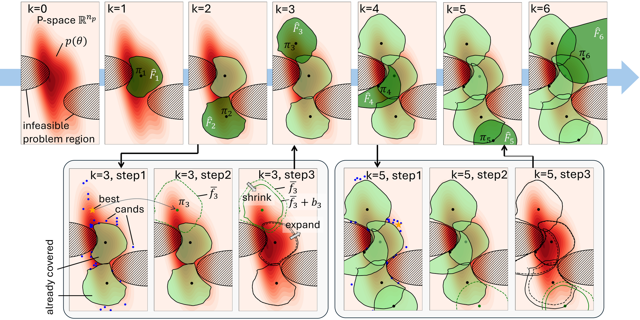
Figure 2: The proposed algorithm actively constructs a library to maximize coverage of $p(\theta)$. For visualization purposes, we assume a one-to-one correspondence between each problem and its solution (experience), thereby allowing experiences (e.g., best, cands, $\pi_{k}$) to be visualized within the P-space. Note that this correspondence is not generally the case. Iterations $k=3$ and $k=5$ are highlighted, and steps 1 to 3 for each iteration are illustrated. Step 1 selects the next experience $\pi_{k}$, which is expected to yield the maximum coverage gain among the candidates. Step 2 trains the base term $\bar{f}_{k}$ via regression. Step 3 determines the bias terms $b_{1:k}$ through optimization to meet the FP rate constraint. During the optimization at step 3 of the $k$-th iteration, regions defined by the base term $\bar{f}_{k}$ (green dashed line) and by previously determined regions (black dashed lines) are either shrunk or expanded to the regions depicted by green or black solid lines.

IV Iterative Algorithm for library construction

This section presents an iterative algorithm, CoverLib, to approximately solve the library construction problem (5).

IV-A Method overview of CoverLib

Problem (5) is challenging due to its combinatorial black-box nature and functional optimization aspect. The combinatorial black-box nature arises from the exponential growth of the search space as the number of experiences increases and the need for Monte Carlo (MC) integration to estimate $r(\cdot)$ and $\alpha(\cdot)$. This makes it intractable to exploit the problem’s structure for optimization. The functional optimization aspect stems from $\hat{f}_{1:k}$, with the optimization variable being functions. To address the combinatorial black-box challenge, we decompose the problem into a sequence of subproblems, thereby forming a greedy iterative algorithm. For the functional optimization challenge, we decompose $\hat{f}_{i}$ into $\hat{f}_{i}=\bar{f}_{i}+b_{i}$, where $\bar{f}_{i}$ is the highly parameterized base term and $b_{i}\in\mathbb{R}$ is the bias term. Here, $+$ can denote the sum of a function and a scalar, treating the scalar as a constant function. We obtain the base term through regression on a dataset generated by $(\theta,c)\sim p(c|\theta,\pi_{i})p(\theta)$, treating only $b_{1:k}$ as the optimization variables in (6).

The adoption of the greedy iteration above is motivated by a well-known fact: the greedy algorithm achieves an efficient $(1-1/e)$-approximation of the optimal solution when the objective function is submodular [26, 27]. Assuming perfect classifiers obtained instantly without any data-generation/training and a finite search space for experiences, the library construction problem (5) is equivalent to the weighted MAX-COVER problem, a well-known example of submodular function maximization. The structural similarity between (5) and the weighted MAX-COVER problem suggests that the greedy approach is effective in practice.

Each iteration consists of three steps: (step 1) heuristically determining $\pi_{k}$ that is expected to have a large coverage gain $r(\hat{f}_{1:k})-r(\hat{f}_{1:k-1})$, which is estimated using the information of $\hat{f}_{1:k-1}(=\{\bar{f}_{i}+b_{i}\}_{i=1}^{k-1})$; (step 2) training the base term $\bar{f}_{k}$ using the dataset generated based on $\pi_{k}$; (step 3) determining the bias terms $b_{1:k}$ by the following optimization:

$$\max_{b_{1:k}}r(\left\{\bar{f}_{i}+b_{i}\right\}_{i=1}^{k}),\;\mathrm{s.t.}\;\alpha(\pi_{1:k},\left\{\bar{f}_{i}+b_{i}\right\}_{i=1}^{k})\leq\delta$$ (6)

where $\pi_{1:k}$ and $\bar{f}_{1:k}$ are fixed in the optimization. Note that the bias terms can be both positive and negative, which respectively make the classification conservative or optimistic. While the first and second steps do not consider the FP rate constraint, the third step does and compensates for its absence in the first two steps. The variable dependencies in each step are roughly as follows:

$$\bar{f}_{1:k-1},b_{1:k-1} \rightarrow\pi_{k},\;$$ (step 1, line 4 of Alg. 1)

$$\pi_{k} \rightarrow\bar{f}_{k},\;$$ (step 2, lines 5-6 10-11 of Alg. 1)

$$\pi_{1:k},\bar{f}_{1:k} \rightarrow b_{1:k}.\;$$ (step 3, line 7 of Alg. 1)

The overall procedure is summarized in Algorithm 1 and an illustration of the algorithm is shown in Fig. 2. The while loop with the breaking condition $\hat{r}_{\mathrm{opt}}>\hat{r}_{\mathrm{pre}}$ is necessary because each iteration does not guarantee an increase in coverage. The following subsections will provide a more detailed explanation of each of the three steps.

procedure: $\mathrm{buildLibrary}(c_{\mathrm{max}},\delta,K)$

tuning param: $\gamma_{\mathrm{init}}$

1 $\hat{r}_{\mathrm{pre}}\leftarrow 0,\gamma\leftarrow\gamma_{\mathrm{init}}$

2 for $k\in 1..K$ do

3      do

4           $\pi_{k},\hat{\Delta}(\pi_{k})\leftarrow\mathrm{determineExperience}(\hat{f}_{1:k-1},c_{\mathrm{max}})$

5           $n_{\mathrm{data}}\leftarrow\gamma/\hat{\Delta}(\pi_{k})$

6           $\bar{f}_{k}\leftarrow\mathrm{trainModel}(\pi_{k},n_{\mathrm{data}})$

7           $b_{1:k},\hat{r}_{\mathrm{opt}}\leftarrow\mathrm{determineBiases}(\pi_{1:k},\bar{f}_{1:k},\delta,c_{\mathrm{max}})$

8          

9     while $\hat{r}_{\mathrm{opt}}\leq\hat{r}_{\mathrm{pre}}$;

10     $\hat{f}_{i}(\theta)\xleftarrow{def}\bar{f}_{i}(\theta)+b_{i},\forall i\in\{1..k\}$

11      $\rho\leftarrow(\hat{r}_{\mathrm{opt}}-\hat{r}_{\mathrm{pre}})/\hat{\Delta}(\pi_{k-1})$

12      update $\gamma$ following the rule (8)

13      $\hat{r}_{\mathrm{pre}}\leftarrow\hat{r}_{\mathrm{opt}}$

14     

return $\pi_{1:K},\hat{f}_{1:K}$

Algorithm 1 CoverLib algorithm

IV-B Next experience $\pi_{k}$ determination (step 1)

This procedure corresponds to $\mathrm{determineExperience}$ in Alg. 1. The purpose of this step is to determine the next experience $\pi_{k}$ that is expected to have a large coverage gain. The actual coverage gain $r(\hat{f}_{1:k})-r(\hat{f}_{1:k-1})$ cannot be computed, as $\hat{f}_{1:k}$ will be determined in the subsequent steps 2 and 3. Instead, the MC estimation of the following quantity is used as an approximation of the true coverage gain:

$$\Delta(\pi):=\mathbb{P}_{(\theta,c)}\left[\theta\notin\cup_{i=1}^{k-1}\hat{F}_{i}\land c\leq c_{\mathrm{max}}\right]$$ (7)

where $(\theta,c)\sim p(c|\theta,\pi)\cdot p(\theta)$. This choice of maximization objective is justified by the fact that maximization of $\Delta(\pi)$ equals maximization of the true coverage gain if $\hat{f}_{1:k}$ are perfect.

The determination of $\pi_{k}$ is then performed by $\operatornamewithlimits{argmax}_{\pi}\Delta(\pi)$ where $\Delta(\pi)$ is estimated by MC integration with $n_{\mathrm{mc}}$ samples. This operation is carried out by random search (RS) with $n_{\mathrm{cand}}$ candidate experiences. In the RS, the choice of the search distribution of $\pi$ is crucial. The adopted search distribution is induced by the following procedures: sample $\theta\sim p(\theta)$ until $\theta\notin\cup_{i=1}^{k-1}\hat{F}_{i}$ (e.g. by sampling by rejection), then solve for such $\theta$ using a from-scratch planner and obtain $\pi$ as the solution. The motivating heuristic behind this choice of the search distribution is the following: Consider a problem $\theta$ and one of its solutions $\pi$. If a new problem $\theta^{\prime}$ is similar to $\theta$, then adaptation of $\pi$ to $\theta^{\prime}$ takes fewer computational costs. This heuristic motivates confining the search space to the uncovered region $(\cup_{i=1}^{k-1}\hat{F}_{i})^{c}$, because such a solution to a problem in the uncovered region is expected to be easily adapted to other problems in the same region.

The procedure is summarized in the pseudo code in Alg. 2. The first while loop defines the search distribution for $\pi$ in the RS. It samples $n_{\mathrm{mc}}$ candidate experiences $\Pi_{\mathrm{cand}}$. The second while loop samples $n_{\mathrm{mc}}$ uncovered problems $\Theta_{\mathrm{uncovered}}$ for MC estimation of $\Delta$. The final for loop computes the expected gain and selects the best experience $\pi_{\mathrm{best}}$. Note that the $\mathrm{fromScratchPlan}(\theta)$ procedure returns the solution path as an experience if successful; otherwise, it returns nil if it fails. It is recommended to use a probabilistic complete planner with sufficient timeout for $\mathrm{fromScratchPlan}$.

procedure: $\mathrm{determineExperience}(\hat{f}_{1:k-1},c_{\mathrm{max}})$

tuning param: $(n_{\mathrm{cand}},n_{\mathrm{mc}})=(100,500)$, these values are fixed throughout this article.

1 $\Pi_{\mathrm{cand}}\leftarrow\{\}$

2 while  $\#\Pi_{\mathrm{cand}}<n_{\mathrm{cand}}$ do

3       $\theta\sim p(\theta)$

4       if $\theta\notin\cup_{i=1}^{k-1}\hat{F}_{i}$ then

5             $\pi\leftarrow\mathrm{fromScratchPlan}(\theta)$

6             if $\pi\neq nil$ then

7                   $\Pi\leftarrow\Pi_{\mathrm{cand}}\cup\{\pi\}$

8                  

9            

10      

11$\Theta_{\mathrm{uncovered}}\leftarrow\{\},n_{\mathrm{total}}\leftarrow 0$

12 while  $\#\Theta_{\mathrm{uncovered}}<n_{\mathrm{mc}}$ do

13       $n_{\mathrm{total}}\leftarrow n_{\mathrm{total}}+1$

14       $\theta\sim p(\theta)$

15       if $\theta\notin\cup_{i=1}^{k-1}\hat{F}_{i}$ then

16             $\Theta_{\mathrm{uncovered}}\leftarrow\Theta_{\mathrm{uncovered}}\cup\{\theta\}$

17            

18      

19$\hat{\Delta}_{\mathrm{best}}\leftarrow 0,\pi_{\mathrm{best}}\leftarrow nil$

20 for $\pi\in\Pi_{\mathrm{cand}}$ do

21       $s\leftarrow 0$

22       for $\theta\in\Theta_{\mathrm{uncovered}}$ do

23             $c\sim p(c|\theta,\pi)$

24             if $c\leq c_{\mathrm{max}}$ then

25                   $s\leftarrow s+1$

26                  

27            

28      $\hat{\Delta}\leftarrow s/n_{\mathrm{total}}$

29       if $\hat{\Delta}>\hat{\Delta}_{\mathrm{best}}$ then

30             $\pi_{\mathrm{best}}\leftarrow\pi,\hat{\Delta}_{\mathrm{best}}\leftarrow\hat{\Delta}$

31            

32      

return $\pi_{\mathrm{best}},\hat{\Delta}_{\mathrm{best}}$

Algorithm 2 Determine next experience to add

IV-C Regression of base term $\bar{f}_{k}$ (step 2)

This step determines the base part $\bar{f}_{k}$ of $\hat{f}_{k}$ by regression. The mean squared error between the predicted and actual computational cost serves as the loss function for regression. The dataset for regression is generated by sampling $n_{\mathrm{data}}$ times from the distribution $(c,\theta)\sim p(c|\theta,\pi_{k})\cdot p(\theta)$. Although any model can be adopted for $\bar{f}_{k}$, as of 2024, neural networks are likely the most suitable choice due to their expressive power and tool availability.

One must carefully consider $n_{\mathrm{data}}$ due to the trade-off between model accuracy and computational cost (data generation and training). Note that an inaccurate model will result in setting the bias term $b_{k}$ to be large in the subsequent step to satisfy the FP rate constraint, leading to a conservative coverage gain compared to the actual gain.

One key observation for adaptively determining $n_{\mathrm{data}}$ is the following: Assume the adaptation algorithm is deterministic for simplicity . Let $R_{k}$ be a region where adaptation of $\pi_{k}$ is successful but not those of $\pi_{1:k-1}$. Then the number of samples in the dataset that fall into $R_{k}$ is proportional to $\Delta(\pi_{k})$ in (7). This observation suggests that as the iteration proceeds, the number of samples falling into the region $R_{k}$ will gradually decrease if $n_{\mathrm{data}}$ remains constant throughout the iterations. To maintain a sufficient number of samples in such a region to preserve accuracy, $n_{\mathrm{data}}$ should be inversely proportional to the coverage gain $\Delta(\pi_{k})$ estimated in step 1; that is $n_{\mathrm{data}}=\gamma/\hat{\Delta}(\pi_{k})$ (line 5 of Alg. 1), where $\gamma$ is an inverse proportionality constant. While this heuristic essentially substitutes the challenge of determining $n_{\mathrm{data}}$ with that of determining $\gamma$, the latter is easier to tune as it reflects the aforementioned observation.

Still, tuning $\gamma$ presents a similar trade-off as tuning $n_{\mathrm{data}}$. To address this, we adopt the following strategy: we set the initial value $\gamma_{1}$ at the beginning and then adaptively change it throughout the iteration according to the achievement rate $\rho_{k}:=(\hat{r}_{k-1}-\hat{r}_{k-2})/\hat{\Delta}(\pi_{k-1})$, which represents the ratio of the actual coverage gain to the estimated coverage gain. A small (near 0) $\rho_{k}$ indicates that $n_{\mathrm{data}}$ should have been larger in the previous iteration; thus, we increase $\gamma_{k}$ and vice versa. We use the following update rule for $\gamma_{k}$ throughout the paper:

$$\gamma_{k}=\begin{cases}\gamma_{k-1}\times 1.1&\text{if $\rho_{k}<0.3$}\\ \gamma_{k-1}\times 0.9&\text{if $\rho_{k}>0.7$}\\ \gamma_{k-1}&\text{otherwise}.\end{cases}$$ (8)

This $\gamma$ update procedure corresponds to lines 10-11 of Alg. 1.

IV-D Bias terms $b_{1:k}$ determination procedure (step 3)

This step determines $b_{1:k}$ by solving (6). The optimization aims to balance the trade-off between coverage gain and FP rate, as larger bias terms result in higher coverage gain but also a higher FP rate and vice versa. $r(\cdot)$ and $\alpha(\cdot)$ are evaluated via MC integrations, making it natural to employ a black-box optimization (BBO) method. As the iteration progresses, the optimization by BBO becomes more challenging due to the increased dimensionality $k$ of the optimization variables and the fact that even small differences in the objective function values become more important. Instead, a simple RS approach is often more effective than BBO for larger $k$. Thus, fixing $b_{1:k-1}$ and optimizing $b_{k}$ (bias for the latest trained classifier) using a simple RS method is effective. We used both approaches in the iterations and selected the better one.

We utilize the Covariance Matrix Adaptation Evolution Strategy (CMAES) [28], a standard BBO method . As CMAES, like most BBO methods, cannot directly handle hard inequality constraints, we reformulate the objective function by incorporating the inequality term as a penalty:

$$J(b_{1:k}) =-r(\left\{\bar{f}_{i}+b_{i}\right\}_{i=1}^{k})$$ (9)

$$+10^{4} ||\mathrm{max}(0,\delta^{\prime}-\alpha(\pi_{1:k},\{\bar{f}i+b_{i}\}_{i=1}^{k}))||^{2}$$

where $\delta^{\prime}$ is set to $\delta-10^{-3}$ to encourage the minimizer to satisfy the inequality constraint, albeit with increased conservativeness. However, this modification does not yet guarantee that the minimizer of $J(b_{1:k})$ will satisfy $\alpha(\cdot)\leq\delta$. To address this issue, we run CMAES 2000 times with different initial seeds, obtaining multiple minimizers of $J(b_{1:k})$ on different local optima. We then select the minimizer that satisfies $\alpha(\cdot)\leq\delta$ and achieves the highest coverage rate $r(\cdot)$.

The MC estimation of $r(\cdot)$ and $\alpha(\cdot)$ in CMAES and RS is computed by $N_{\mathrm{cover}}/N_{\mathrm{mc}}$ and $N_{\mathrm{fp}}/N_{\mathrm{cover}}$, respectively, where

$$N_{\mathrm{cover}}=\sum_{j=1}^{N_{\mathrm{mc}}}\mathbbm{1}\{\min_{i\in\{1..k\}}(\overline{c}^{(i,j)}+b_{i})\leq c_{\mathrm{max}}\}$$ (10)

$$N_{\mathrm{fp}}=\sum_{j=1}^{N_{\mathrm{mc}}}\mathbbm{1}\{i^{\prime}=\operatornamewithlimits{argmin}_{i\in\{1..k\}}(\overline{c}^{(i,j)}+b_{i}),$$ (11)

$$\qquad\qquad\qquad\bar{c}^{(i^{\prime},j)}+b_{i^{\prime}}\leq c_{\mathrm{max}}\land c^{(i^{\prime},j)}\leq c_{\mathrm{max}}\}.$$

Here $c^{(i,j)}$ is a sampled value from $p(c|\theta^{(j)},\pi_{i})$ and $\bar{c}^{(i,j)}$ is the evaluation of $\bar{f}_{i}(\theta^{(j)})$. Although sampling from $p(c|\theta^{(j)},\pi_{i})$ is computationally expensive as it performs actual adaptation, it is possible to share $\{c^{(i,j)}\}_{i=1,j=1}^{k,N_{\mathrm{mc}}}$ and $\{\bar{c}^{(i,j)}\}_{i=1,j=1}^{k,N_{\mathrm{mc}}}$ across the CMAES and RS iterations, because only $b_{1:k}$ is optimized and the others are fixed.

We further reduce the computational cost by sharing the problem set $\Theta_{\mathrm{mc}}=\{\theta^{(j)}\}_{j=1}^{N_{\mathrm{mc}}}$ across all $k\in[K]$ iterations. We can cache the values of $c^{(i,j)}$ and $\bar{c}^{(i,j)}$ for all $i\in[k]$ and $j\in[N_{\mathrm{mc}}]$, and reuse them in step 3 in the subsequent iterations (i.e. $k+1\ldots$-th iterations in Alg. 1). This caching technique reduces the total number of samples from $p(c|\theta,\pi)$ from $K(K-1)N_{\mathrm{mc}}/2$ to $KN_{\mathrm{mc}}$. Throughout this article, a large value of $N_{\mathrm{mc}}=10^{4}$ is used to ensure the accuracy of the MC estimation, but this does not become a computational bottleneck thanks to the above caching techniques.

IV-E Reduce computational time through large parallelization

The proposed algorithms may experience bottlenecks in five procedures: 1) sampling from $p(\theta)$, 2) sampling from $p(c|\theta,\pi)$ which involves the adaptation operation, 3) $\mathrm{fromScratchPlan}$ procedure, 4) $\mathrm{runCMAES}$ procedure, and 5) training the base term $\bar{f}_{k}$ through regression. Fortunately, the first four procedures can be easily parallelized. In our implementation, we evenly distribute these tasks across two servers (see Sec. V-E) where each server has a worker pool. Parallelizing these procedures significantly reduces the computational time. Although the last $\bar{f}$ training procedure could also be parallelized using distributed training techniques, we did not implement this in the current study.

V Shared settings and implementation details in numerical experiments

V-A Baseline: passive random sampling nearest neighbor search library

For comparison of the high-level parts of the library-based methods, we adopt a baseline approach called NNLib, which utilizes passive random sampling for library construction and nearest neighbor search for querying. As reviewed in Section II-A, most library-based planning algorithms adopt an NNLib-style approach or its variants. The NNLib is constructed by repeating the following process: sampling $\theta\sim p(\theta)$ then solving it from scratch using a global planner with a sufficient time budget. If the problem is solved, the experienced solution $\pi$ is stored in the library with the key $\theta$. Here, for a fair comparison, the global planner and its timeout are set to be the same as in CoverLib (i.e. $\mathrm{fromScratchPlan}$). During the online planning phase, given the P-parameter $\theta_{\mathrm{q}}$, the solution of the nearest key to $\theta_{\mathrm{q}}$ is retrieved from the library. Our NNLibs’s query implementation employs a ball-tree [30] to enable efficient query search. Hereinafter, when we refer to the library size of NNLibs, it represents the number of solved problems used to construct the library rather than the number of stored experiences in the library.

For the baseline, we constructed NNLib with two distinct features: NNLib(full), which uses the full dimension of $\theta$ for the query, and NNLib(selected), which uses only the initial and goal condition-related components of $\theta$. Examples of such components include the initial base pose and reaching target coordinates. This feature selection is motivated by previous research [9, 10], which shows that using only the initial and goal conditions as the query remains effective even if the environment changes. As NNLib is expected to be susceptible to the curse of dimensionality, such a feature selection can potentially improve its performance.

V-B On Islam et al.’s approach as a potential baseline

The work [11, 12] by Islam et al. reviewed in Section II-B is another potential baseline method. Although applicable to all settings in the numerical experiments with minor modifications, we omitted it from the comparison for the following reasons. Their approach requires discretization. Even in Task 2 (see Section VI-C), with the 10-dimensional P-space being the lowest among the Tasks in Section VI, the computational cost would be significant with coarse discretization (e.g., 10 bins per dimension). Suppose a single adaptation takes 0.1 seconds and we consider using the two ARM-servers (in total 156 cores) stated in Section V-E for fully parallel processing. Checking the adaptability of the selected experience path for all $10^{10}$ possible problems would take $10^{10}\cdot 0.1/156/3600/24=74$ days at the first iteration. Repeating a similar process many times to populate the library would require an immense amount of computational time. The computational challenge worsens exponentially for Task 1 and Task 3, which have dozens of dimensions. This is why we did not consider their approach in the comparison.

V-C Adaptation algorithms

For both NNLib and CoverLib, we are free to choose the low-level part, that is, the adaptation algorithm. In this paper, we consider the following two adaptation algorithms from different categories: one from the a) NLP-based category and another from the b) SBMP-based category. Algorithm a) is a general-purpose algorithm, while algorithm b) is more suitable for unconstrained path planning problems; thus, we applied them accordingly. We describe the specific implementation details of the algorithms (SQPPlan and ERTConnect) corresponding to both categories in the following.

a) Sequential Quadratic Programming based planning (SQPPlan): Most motion planning problems can be formulated as constrained NLPs. Adaptation of a specific experience $\pi$ can be done straightforwardly in this framework by solving the optimization problem with $\pi$ as the initial guess of the solution. We adopt sequential quadratic programming (SQP) as the optimization algorithm. The computation cost $c$ for SQPPlan is measured by the outer iteration count, not the iteration count of the internal QP solver. To exploit the sparse block structure in the trajectory optimization, we use OSQP [31] as the internal QP solver. Note that our SQP implementation is simplified; line-search and trust-region are omitted, and the Hessian of the constraints is ignored.

b) Experience-driven random tree connect (ERTConnect): Experience-driven random tree connect (ERTConnect) [10] is the state-of-the-art sampling-based adaptation algorithm. In addition to its speed and broad adaptability, ERTConnect excels in path quality without requiring path simplification, unlike the approach used in Lightning [9]. Therefore, we used ERTConnect without any path simplification. As ERTConnect is a bidirectional algorithm, it requires determining the path’s terminal configuration in advance. Determining the terminal configuration from scratch is computationally expensive, as it involves solving the constrained inverse kinematics (IK) with multiple initial guesses, which often takes a comparable amount of time to the path planning itself. To address this, our implementation takes advantage of the terminal configuration of the retrieved experience as the initial guess. If the IK failed with that initial guess, the entire planning process was considered a failure. The constrained-IK is implemented using scipy’s [32] implementation of SQP (referred to as scipy-SQP). The computation cost $c$ for ERTConnect is measured by the number of collision checks inside the path-planning algorithm ignoring the ones in the IK solver.

V-D Modeling and regression of the base term $\bar{f}$

We model the base term $\bar{f}$ using a neural network architecture. We consider two types of modeling: vector modeling and vector-matrix modeling. For vector modeling, a single fully connected neural network (FCN) is used. The FCN takes a vector-formed P-parameter $\theta$ as input and outputs the expected value $\bar{c}$ of the computational cost. For vector-matrix modeling, we split the P-parameter $\theta$ into the matrixable part $\theta_{\mathrm{mat}}$ and the other vector part $\theta_{\mathrm{other}}$. Figure 3 illustrates the vector-matrix modeling. The matrixable part refers to the portion of the P-parameter that can be well represented by a matrix. The conversion from $\theta_{\mathrm{mat}}$ to a matrix is done by an embedding function $\phi_{\mathrm{emb}}$, which is procedurally defined and not learned. A typical example of the matrixable part is a parameter for the cluttered workspace, which is often represented as a heightmap or a signed distance field. The matrix is then encoded by a Convolutional Neural Network (CNN) into a high dimensional vector, while an FCN (FCN1) enlarges $\theta_{\mathrm{other}}$ to match the order of its dimension to that of the CNN. Then, the outputs of both networks are concatenated and processed by another FCN (FCN2). Note that one can adopt other embeddings appropriate for a particular problem setting, such as a point cloud, voxel grid, or graph structure, although exploring these options is outside the scope of this article.

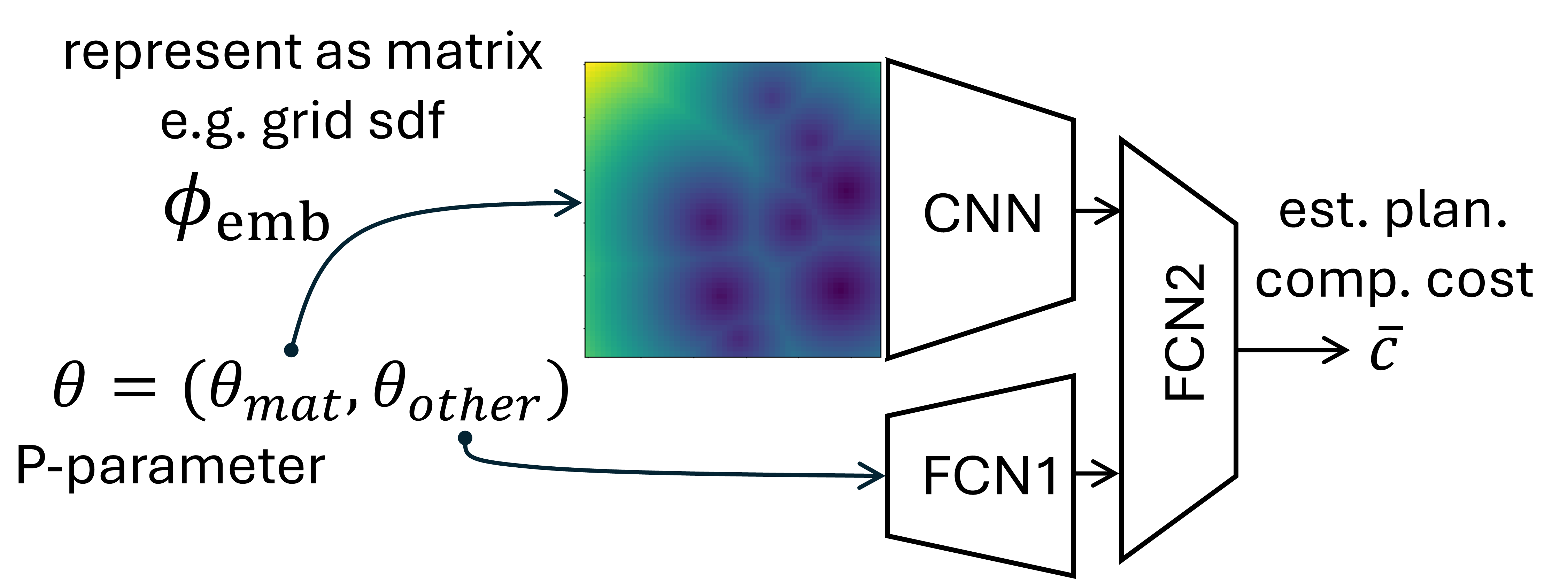
Figure 3: Illustration of vector-matrix modeling.

The CNN used in the vector-matrix modeling can be pretrained in a self-supervised manner by preparing an hourglass-shaped CNN AutoEncoder and minimizing the reconstruction loss between the input and output. During training of $\bar{f}$, we fix the CNN encoder part and only train the FCN part, discarding the decoder part afterwards. Utilizing a fixed pretrained encoder significantly reduces both the training and inference time of $\bar{f}$. The inference time is reduced because the encoder part is shared among all the functions $\bar{f}_{1:K}$ in the library, meaning the CNN encoder part is evaluated only once instead of $K$ times.

For more details on the network architectures, training, and inference settings, please refer to Appendix V-D.

V-E Computational resources

For the experiments, we utilized two ARM-servers (ARM Neoverse N1 80-Core, 256GB DRAM, 3.3GHz) and a single desktop PC (AMD Ryzen 9 3900X 12-Core with SMT, 64GB DRAM, 3.8GHz, GeForce RTX 2080 Ti). Please note that Neoverse N1 is a server-grade processor and is not for consumer use. During the preprocessing phase, both ARM-servers and the desktop PC were employed. As stated in IV-E, most of the time-consuming procedures, except fitting $\bar{f}$, can be parallelized. Hence, we performed parallelizable computations on each ARM-server using 78 parallel processes (-2 for other purposes), totaling 156 processes. In contrast, during the benchmarking phase, only the desktop PC was used, with a single physical core (i.e., 2 logical cores) isolated from the Linux process scheduling.

VI Numerical Experiment

VI-A Benchmarking Methodology

We conduct numerical experiments to evaluate the proposed method in three different motion planning problem domains, focusing on the following two aspects:

Planning Performance Comparison (PPC): We compare the performance of CoverLib against three other methods: a global planner (referred to as Global), NNLib(full) and NNLib(selected). The Global is supposed to be a probabilistically complete algorithm, meaning that given enough time, it can find a solution if one exists. While CoverLib and NNLibs are not expected to achieve the same level of success rate as Global, our aim is to evaluate how closely they can approach this upper bound while requiring less planning time.

Note that the success rate does not often provide a comprehensive picture of a method’s ability to handle difficult problems. In a typical domain, the majority of problems are often easy, while a smaller subset of problems, usually in specialized or niche areas of the P-space, are considerably more challenging. As a result, the overall success rate may be skewed towards the performance on easier problems. To better gauge the capability of each method, we introduce a new metric called Global Planner Equivalent Timeout (GPE-TO). GPE-TO represents the timeout value at which Global achieves the same success rate as the method being evaluated. To calculate GPE-TO, we first preprocess the benchmark results of Global to create a mapping between timeout values and their corresponding success rates (see plots for Global in Fig. 13). Then, for each method, we find the timeout value in this mapping that corresponds to the method’s success rate. For each domain, we benchmark the methods using 3000 problems sampled from $p(\theta)$. Then, we compare three key aspects: GPE-TO, success rate, and planning time.

Library Growth Comparison (LGC): Alongside the PPC, we perform a Library Growth Comparison (LGC) to assess the evolution of CoverLib and NNLib’s success rates as their libraries grow. While PPC provides a snapshot of the methods’ performance at a specific library size, LGC offers a comprehensive picture of efficiency in library construction by plotting the success rate growth for each library-based method as the library construction time increases. NNLib’s success rate growth curve is computed by measuring the success rate in the same manner as in the PPC with different library sizes. The CoverLib’s counterpart is obtained from the cached values in the library construction process. At each iteration of library construction, we approximate the success rate using $(1-\delta)\hat{r}_{\mathrm{opt}}$, where $\hat{r}_{\mathrm{opt}}$ is obtained by determineBiases function in Algorithm 1 line 7. This value $(1-\delta)\hat{r}_{\mathrm{opt}}$ represents an estimated lower bound of the success rate using $N_{\mathrm{mc}}=10^{4}$ samples.

In the plots for both PPC and LGC, the approximate upper bound of the success rate of the domain is indicated by a red horizontal line. This upper bound is estimated by running Global with a sufficiently large (180 sec) timeout for 3000 problems randomly sampled from $p(\theta)$. It’s important to note that this upper bound does not reach 100% even with an infinite timeout in general, as some problems in the domain can be infeasible.

VI-B Task 1: Kinodynamic planning for double integrator

Domain definition ($n_{\mathrm{p}}=32$): Two dimensional double integrator is a simple dynamical model described by a linear system $\ddot{x}=u$, where $x\in\mathbb{R}^{2}$ is the position and $u\in\mathbb{R}^{2}$ is the acceleration control input. We consider a $[0,1]\times[0,1]$ square-shaped world with 10 randomly placed $\in\mathbb{R}^{10\times 2}$ circular obstacles of random radii $\in\mathbb{R}^{10}$. The start $v_{\mathrm{start}}$ and goal $v_{\mathrm{goal}}$ velocities are both fixed at $(0,0)$. The velocity and acceleration are bounded by $||\dot{x}||_{\infty}\leq 0.3$ and $||u||_{\infty}\leq 0.1$. The goal position $x_{\mathrm{goal}}\in\mathbb{R}^{2}$ is randomly sampled but the start position is fixed $x_{\mathrm{goal}}=(0.1,0.1)$. Therefore, in total the dimension of the P-space is $n_{\mathrm{p}}=32$. The kinodynamic (kinematic + dynamic) motion planning problem for the double integrator is defined as finding a sequence of control inputs $u_{1},u_{2},\ldots,u_{N-1}$ that satisfies the following constraints:

$$x_{1}=x_{\mathrm{start}},\dot{x}_{1}=\dot{x}_{\mathrm{start}},x_{N}=x_{\mathrm{goal}},\dot{x}_{N}=\dot{x}_{\mathrm{goal}}$$ (12)

$$\dot{x}_{i+1}=\dot{x}_{i}+u_{i}\Delta t,\quad\forall i\in[N-1]$$ (13)

$$x_{i+1}=x_{i}+\dot{x}_{i}\Delta t+u_{i}\Delta t^{2}/2,\quad\forall i\in[N-1]$$ (14)

$$\text{sdf}(x_{i})\geq 0,\quad\forall i\in[N]$$ (15)

$$x_{i}\in[0,1]\times[0,1],||\dot{x}_{i}||_{\infty}\leq 0.3,\quad\forall i\in[N]$$ (16)

$$||u_{i}||_{\infty}\leq 0.1,\quad\forall i\in[N-1]$$ (17)

where $\Delta t$ is the time step and we set $\Delta t=0.3$. $N$ is the number of discretization points. While $N$ is fixed for trajectory optimization, it varies for sampling-based planners. The $\mathrm{sdf}$ is the signed distance function (SDF).

Adaptation algorithm: We adopt SQPPlan as the adaptation algorithm. The trajectory optimization problem is constructed by direct transcription [33] with $N=200$ discretization points with time step $\Delta t$. The cost function is the sum of squared control input: $\sum_{i=1}^{N-1}||u_{i}||^{2}$ and the constraints are given by (12)-(17).

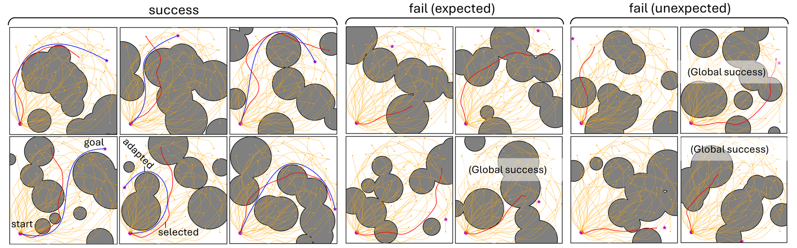
Figure 4: This figure visualizes the behavior of the CoverLib-aided planning with $(c_{\mathrm{max}},\delta)=(5,0.05)$ in Task 1. The Yellow lines are the experiences in the library, while the red line is the selected experience used in adaptation. The blue line shows the result of adaptation. The purple circle and star denote the start and goal positions respectively. The blue line is not shown for failure cases as the result is not obtained. The label “fail(expected)” indicates cases where $\mathrm{min}_{i\in[K]}\hat{f}_{i}(\theta)>c_{\mathrm{max}}$, meaning failure is somewhat expected before adaptation. The label “fail(unexpected)” signifies that adaptation failed even though $\mathrm{min}_{i\in[K]}\hat{f}_{i}(\theta)\leq c_{\mathrm{max}}$. The overlaid ”Global success” label for failed cases suggests that the problem is actually feasible, as evidenced by the success of Global.

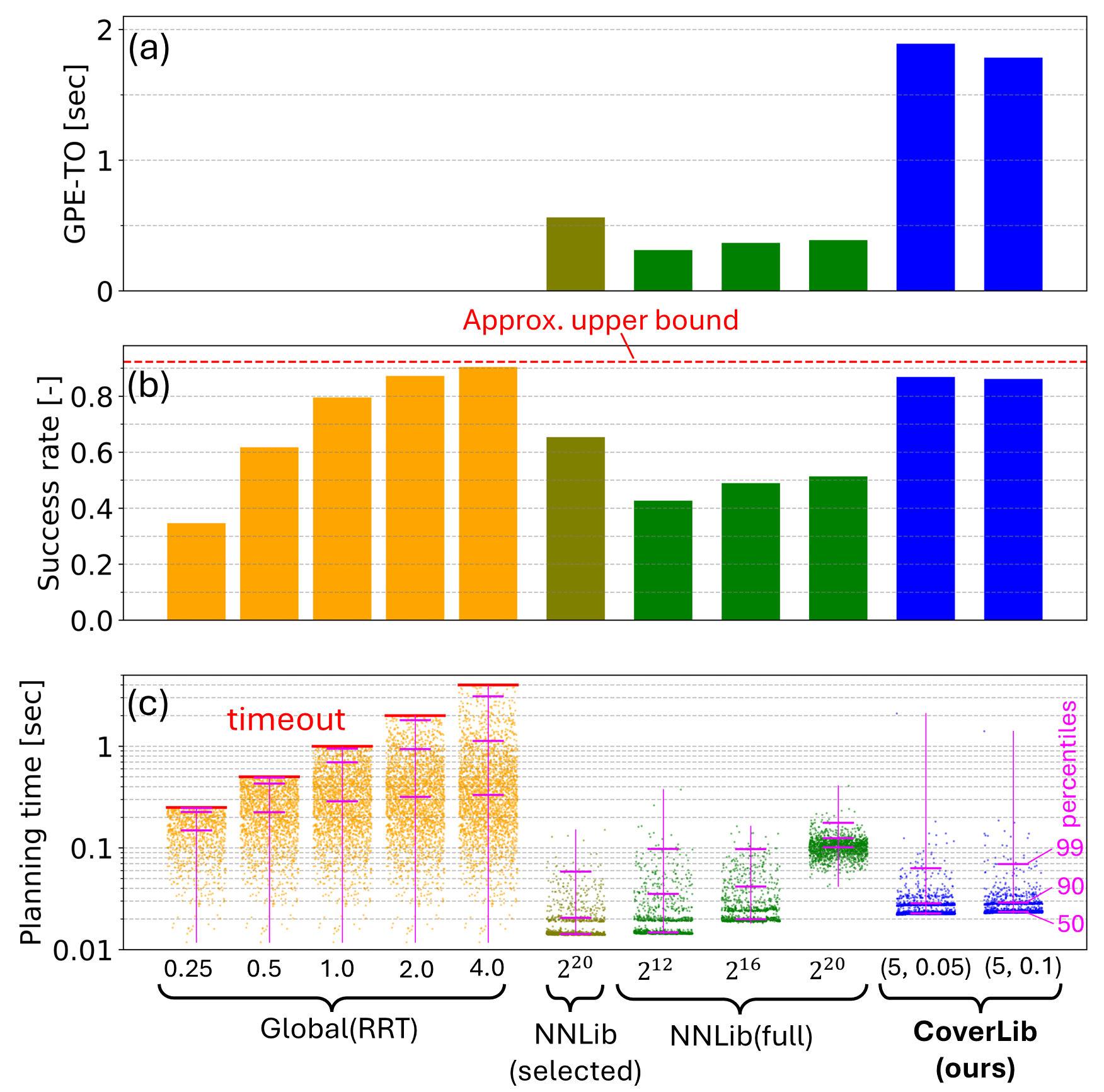
Figure 5: Benchmarking in terms of (a) GPE-TO, (b) Success rate, (c) Planning time for Task 1. The values associated with the Global plot (e.g. 0.25, 0.5, …) represent timeout values. The value associated with NNLib (e.g. $2^{20}$) indicates the library size. The values associated with CoverLib, e.g. (5, 0.05), are $(c_{\mathrm{max}},\delta)$ pairs. In (c), the x-coordinate of each point in the scatter plot represents the problem index, while the y-coordinate represents the corresponding planning time. Data points for problems with failure are not plotted. The vertical pink lines indicate the minimum and maximum planning time of the scatter plot. The three horizontal pink lines along each scatter plot indicate the 50, 90, and 99 percentiles of the planning time. These percentile computations only consider successful cases. The approx. upper bound in (b) is computed as described in Section VI-A.

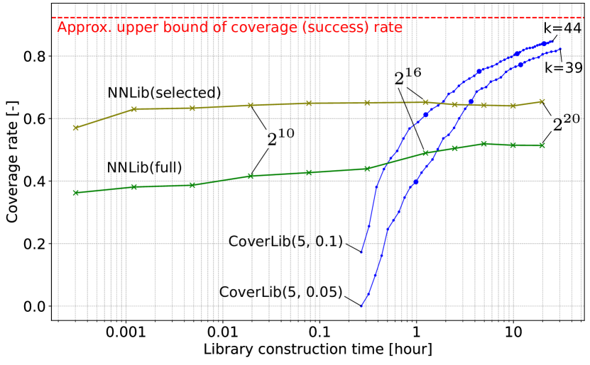
Figure 6: Comparison of library growth for Task 1. For NNLib, the library size is varied as $2^{i}$ for $i\in$ (4, 6, 8, 10, 12, 14, 16, 17, 18, 19, 20), where $2^{20}=1,048,576$. The corresponding library construction time to achieve each specific library size is calculated from the logging results. To ensure a fair comparison, the data generation for the NNLibs is performed using the two ARM-servers mentioned in Section V-E. For CoverLib, the MC estimated lower bound $(1-\delta)\cdot\hat{r}_{\mathrm{opt}}$ of the success rate is plotted for each iteration $k$. Every 10th point is emphasized with a larger marker. The approx. upper bound is computed as described in Section VI-A. Note that the pre-training time for the CNN encoder is included in the library construction time.

From-scratch planner: We adopt the fast marching tree (FMT^∗) [34] for $\mathrm{fromScratchPlan}$, where an analytical time-optimal connection is used to connect the nodes [35]. The FMT^∗ is run with a sufficiently high number of samples, $N=3000$, to find a feasible path. Single planning by this setting typically takes several seconds.

Computational cost predictor: We adopt the vector-matrix modeling for $\bar{f}$. The map $\phi_{\mathrm{emb}}$ takes the list of center-radius pairs of the circular obstacles and returns a $56\times 56$ matrix for the grid map of the SDF. The CNN encoder is pre-trained as described in section V-D. The pre-training time including dataset generation was about 13 minutes.

Result: The library is constructed with $(c_{\mathrm{max}},\delta)=(5,0.1)$ with about 1 day budget and $(5,0.05)$ within about 1.5 days budget. Tuning parameter $\gamma$ is set to 5000. The behavior of planning with the learned CoverLib is visualized in Fig. 4. The CoverLib with SQP adaptation is benchmarked against the baselines: Global, NNLib(full), and NNLib(selected). We adopt RRT as Global. However because straightforward extension of RRT to kinodynamic planning [2] results in a quite slow planning time, we adopt an analytical time-optimal connection [35] between the nodes as did for the scratch planner. The results of PPC and LGC are shown in Fig. 5 and Fig. 6 respectively.

VI-C Task 2: kinematic planning for 31-DOF legged humanoid robot

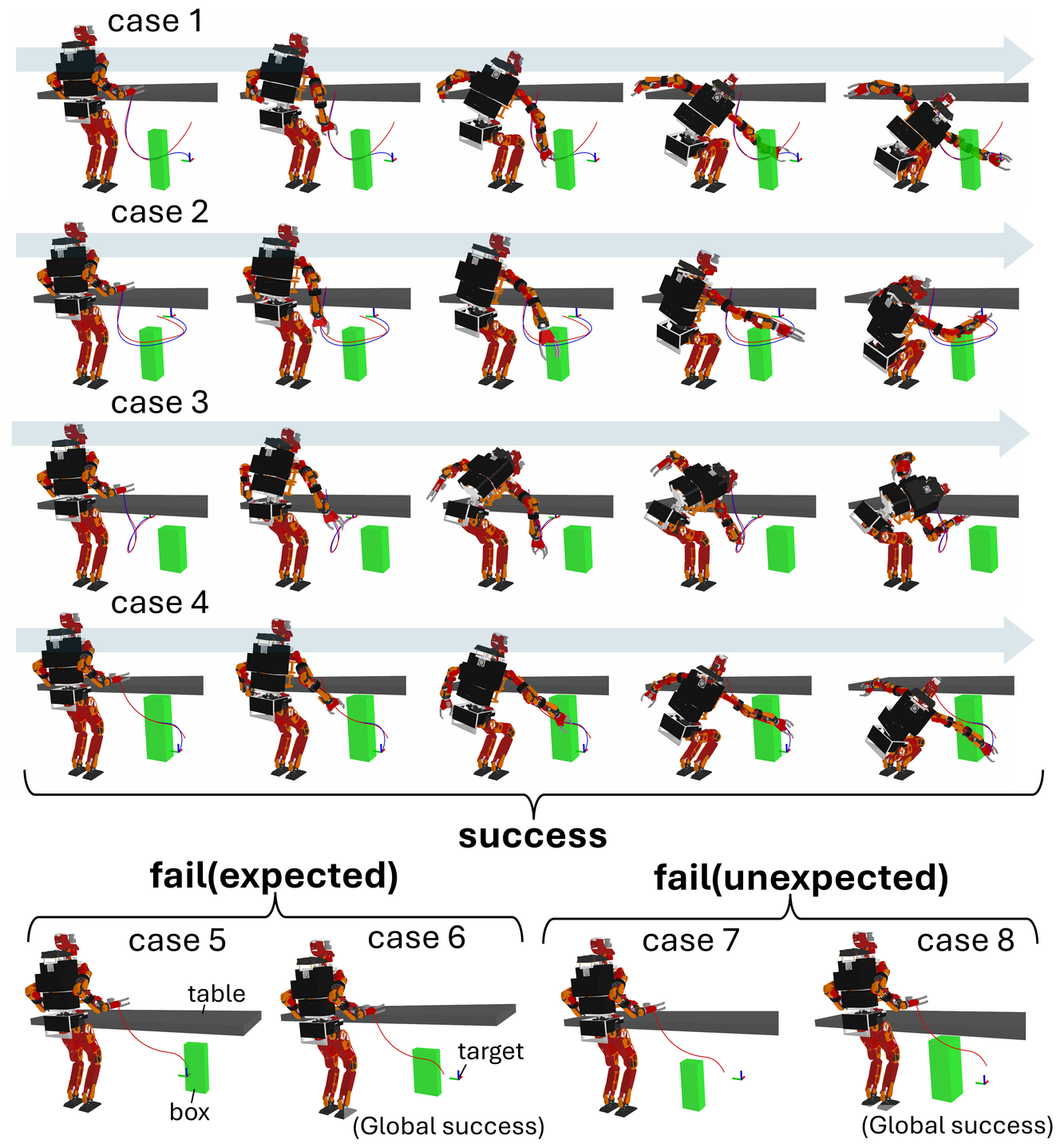
Figure 7: This figure visualizes the behavior of the CoverLib-aided planning with $(c_{\mathrm{max}},\delta)=(5,0.1)$ in Task 2. The red line indicates the selected experiences from the library. The blue line is the result of adaptation. These lines are obtained by mapping the configurations to the end effector positions. See the caption of Fig. 4 for the meaning of fail(expected), fail(unexpected), and (Global success) labels.

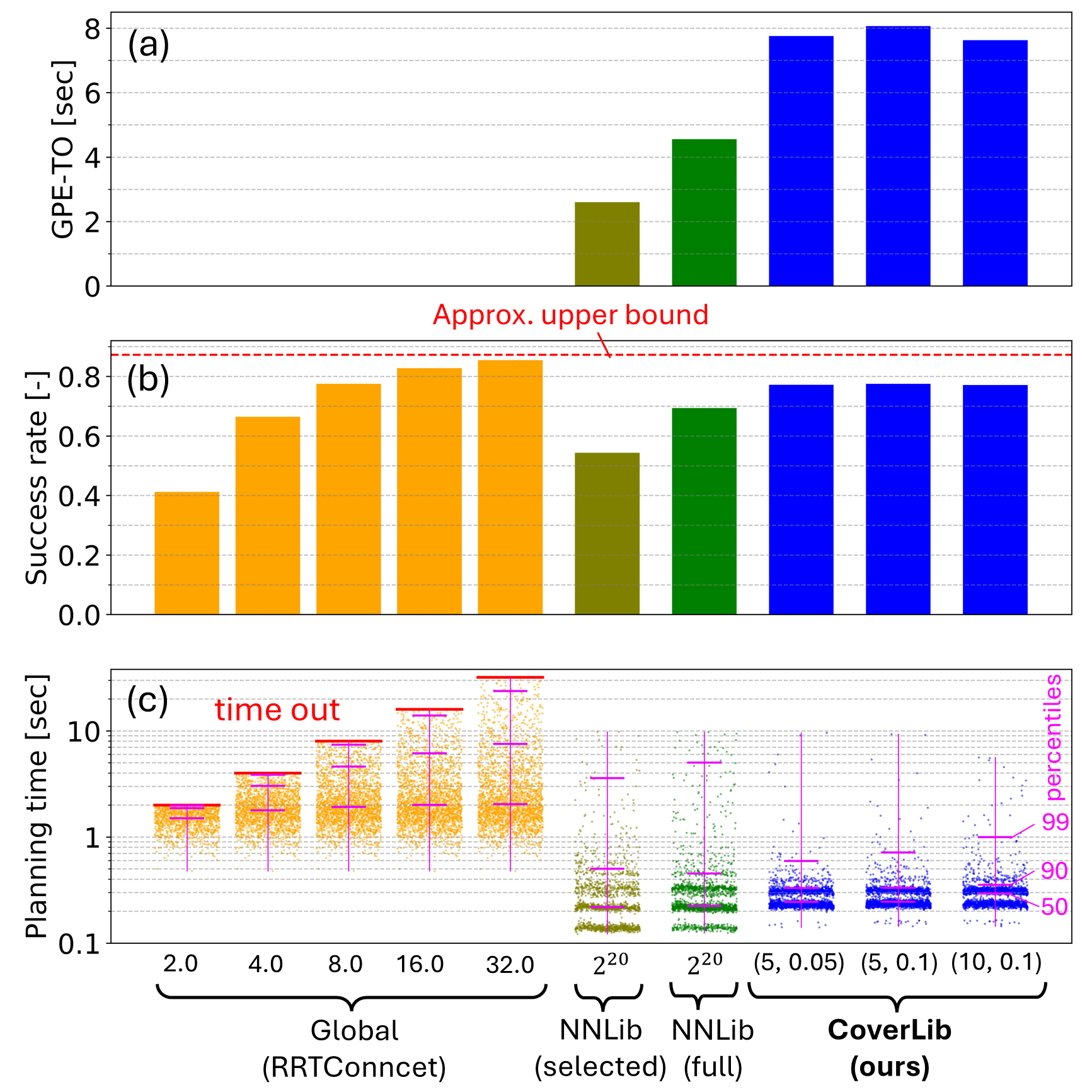
Figure 8: Planning performance comparison for Task 2. Please see the caption of Fig. 5 for the details.

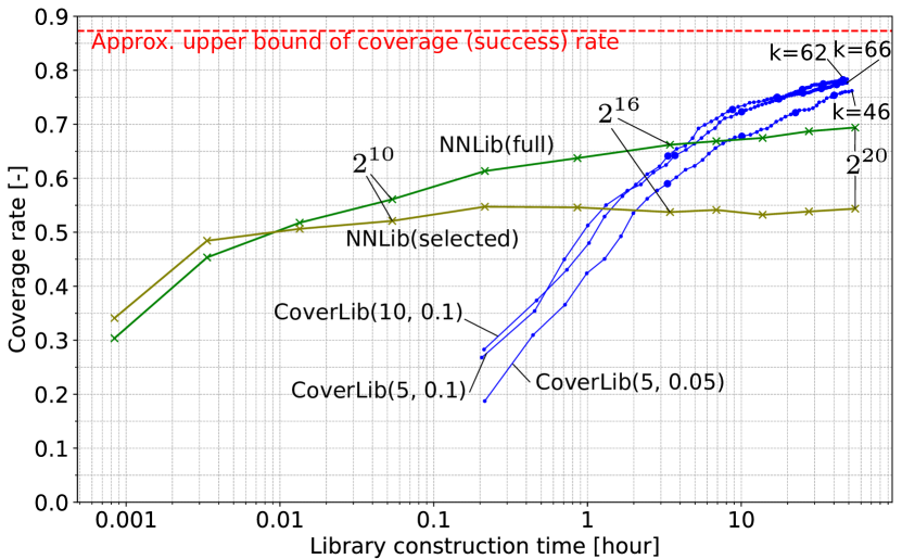
Figure 9: Library growth comparison for Task 2. Please see the caption of Fig. 6 for the details.

Domain definition ($n_{\mathrm{p}}=10$): The humanoid robot we consider is a 31-DOF (arms + legs + torso) robot JAXON [36]. We consider the fully kinematic motion planning problem for the humanoid robot. The robot collision shape is approximated as a set of many spheres covering the robot body. Then, the collision check is efficiently done by SDF evaluation at each sphere position, similar to [3, 37]. We consider a task where the robot reaches its hand to the target position while avoiding the following two obstacles. A fixed-size floating table-like obstacle is placed in the workspace, and its x and z positions $\in\mathbb{R}^{2}$ are randomly sampled. Also, a box-shaped obstacle is placed under the “table”. The obstacle shape $\in\mathbb{R}^{3}$ and its planar position $\in\mathbb{R}^{2}$ are randomly sampled. The target reach position $x_{\mathrm{reach}}\in\mathbb{R}^{3}$ is also randomly sampled in the workspace. Therefore, the dimension of P-space is $n_{\mathrm{p}}=10$. The motion planning problem is defined as finding a sequence of robot configurations $q_{1:L}$ that satisfies the following constraints:

$$q_{1}=q_{\mathrm{start}}$$ (18)

$$endEffectorPosKin(q_{L})=x_{\mathrm{reach}}$$ (19)

$$f_{\mathrm{sdf}}(spherePosKin_{j}(q_{i}))>0,\forall i\in[L],j\in[N_{\mathrm{sphere}}]$$ (20)

$$q_{i}\in JointLimit,\forall i\in[L]$$ (21)

$$comPos2dKin(q_{i})\in supportPolygon,\forall i\in[L]$$ (22)

$$leftLegKin(q_{i})=(x_{l},Q_{1}),\forall i\in[L]$$ (23)

$$RightLegKin(q_{i})=(x_{r},Q_{1}),\forall i\in[L]$$ (24)

$$||q_{i+1,j}-q_{i,j}||\leq\lambda_{j},\forall i\in[L-1],\forall j\in[N_{\mathrm{joint}}]$$ (25)

Note that (22) enforces the ground-projected center of mass of the robot to be inside the support polygon to prevent the robot from falling down. This constraint is treated as an inequality constraint. (23) and (24) enforce the left and right foot to be on the ground at specific coordinates $(x_{l},Q_{1})$ and $(x_{r},Q_{1})$ respectively. (25) enforces the pairwise distance of the each joint to be less than $\lambda_{j}$, which essentially defines the collision check resolution.

Adaptation algorithm: We adopt the SQPPlan for the adaptation algorithm. The objective of the NLP problem is to minimize the sum of squared joint accelerations $\sum_{i=2}^{L-1}(q_{i+1}-2q_{i}+q_{i-1})^{2}$ while satisfying constraints (18)-(25). The length of the trajectory $L$ is set to 40.

From-scratch planner: We adopt a RRTConnect planner for $\mathrm{fromScratchPlan}$ with the following modifications. The equality constraints (23) and (24) make the C-space no longer a simple Euclidean space, but a constrained manifold. Planning on a constrained manifold is known to be challenging and is an active research field [38]. Basically, we use an existing projection-based approach [38]. However, the existing approach solely targets satisfying the equality constraints in the projection. This often results in infeasibility in terms of the inequality constraints, and ends up repeating the projection process in vain as discussed in our recent article [39]. This problem typically occurs in humanoid planning problems, where severe inequality constraints are imposed, such as the support polygon constraint. To satisfy both equality and inequality constraints, we adopt a projection operator that satisfies both of these constraints using SQP. The goal configuration for RRTConnect is determined by a scipy-SQP-based IK that takes into account the constraints (19)-(24). We applied SQPPlan adaptation (the adaptation algorithm works as a path smoother given a non-smooth path) to the RRTConnect’s solution to smooth it out. The time budget for IK + RRTConnect + smoothing is 180 seconds in total.

Cost predictor: As the environment includes only a single object, we adopt the vector modeling for $\bar{f}$.

Result: The CoverLibs are constructed with multiple settings $(c_{\mathrm{max}},\delta)=(5,0.05),(5,0.1),(10,0.1)$ with approximately 2 days budgets. The tuning parameter $\gamma$ is set to 10000.

The performance is compared with the baselines Global, NNLib(full), and NNLib(selected), where Global is RRTConnect, the same as the $\mathrm{fromScratchPlan}$, but without smoothing. The behavior of planning with the learned CoverLib is visualized in Fig. 7. The results of the PPC and LGC are shown in Fig. 8 and Fig. 9 respectively.

VI-D Task 3: Kinematic planning for 10-DOF mobile manipulator

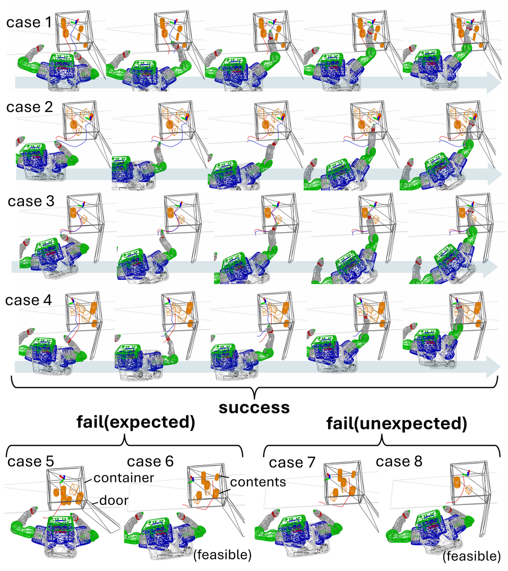
Figure 10: This figure visualizes the behavior of the CoverLib-aided planning with $(c_{\mathrm{max}},\delta)=(2000,0.2)$ in Task 3. See the caption of Fig. 7 for the details.

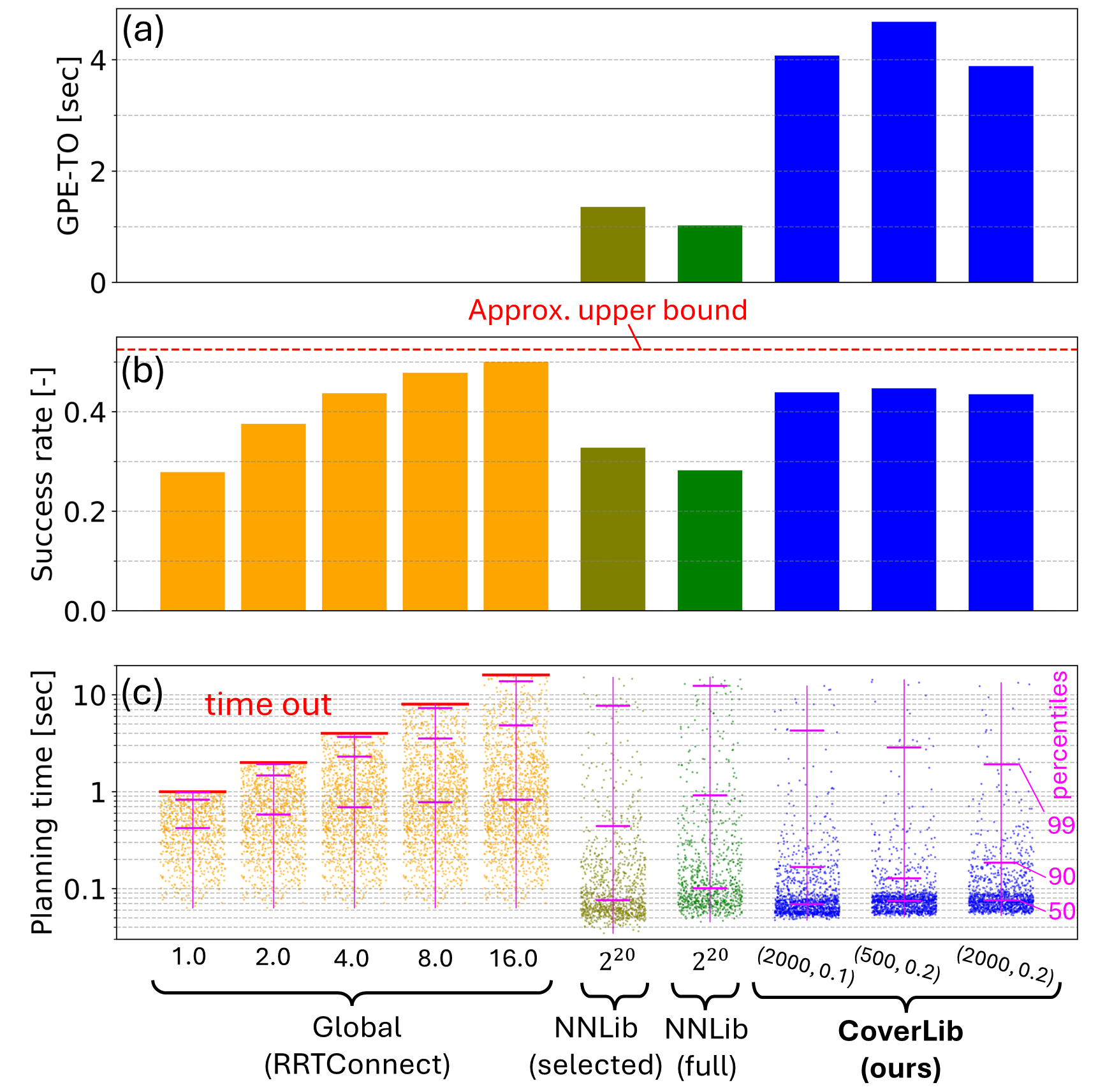
Figure 11: Planning performance comparison for Task 3. Please see the caption of Fig. 5 for the details.

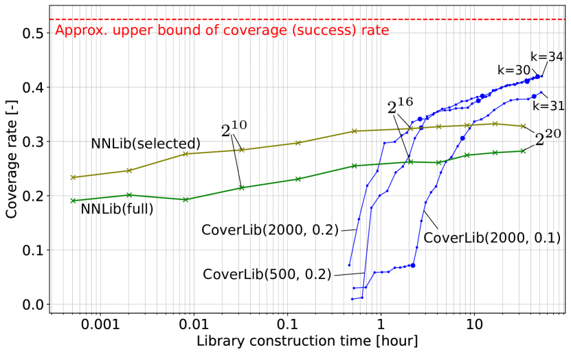
Figure 12: Library growth comparison for Task 3. Please see the caption of Fig. 6 for the details. Note that the end of the CoverLib plots tends to be smaller than the actual success rate in Fig. 11. This is because the plot for CoverLib is a lower bound of the success rate as described in Section VI-A. Note that the pre-training time for the CNN encoder is included in the library construction time.

Domain definition ($n_{\mathrm{p}}=87$): We consider the mobile manipulator robot PR2, using the 7-DOF right arm of the PR2 and hypothetically considering the mobile base as a 3-DOF mobile base. Collision checking is done similarly to Task 2. The task is to reach the right hand to a target position inside a container while avoiding obstacles inside the container. The container has a fixed shape, but the door angle $\in\mathbb{R}$ is randomly changed. A maximum of 10 obstacles are placed inside the container with random size and position. The obstacle is either a box or a cylinder with random size ($\in\mathbb{R}^{3}$ or $\in\mathbb{R}^{2}$) and planar coordinate ($\in\mathbb{R}^{3}$ or $\in\mathbb{R}^{2}$), where the yaw angle is considered only for the box coordinates). The number of obstacles is randomly sampled from 1 to 10. Considering a discrete variable indicating whether each obstacle is a box or a cylinder, the environmental part of the P-parameter is $10\times(1+\max\{3+3,2+2\})=70$ dimensional in total. The starting base planar coordinate $\in\mathbb{R}^{3}$ is randomly sampled near the container. The target coordinate $\in\mathbb{R}^{4}$ is randomly sampled within the container, with only the x, y, z and yaw angles changed. Thus, the dimension of the P-space is $n_{\mathrm{p}}=87$ in total. The motion planning problem is defined similarly to the humanoid problem, without the humanoid-specific constraints (22), (23) and (24).

Adaptation algorithm: We adopt ERTConnect as the adaptation algorithm. While the original ERTConnect [10] set the malleability bound $\varepsilon$, which is the core tuning parameter, to relatively large value 5.0 to cover the entire robot’s kinematic range, we set it to 0.1 to make the algorithm more focused around the experienced trajectory.

From-scratch planner: We adopt the RRTConnect implementation of OMPL [40] with default settings for $\mathrm{fromScratchPlan}$. As in Section VI-C, the goal configuration for RRTConnect is determined by solving collision-aware inverse kinematics (IK) using scipy-SQP until the feasible goal configuration is found. The solution is simplified by the shortcut algorithm in OMPL. The time budget for IK + RRTConnect + simplification is 30 seconds in total.

Cost predictor: We adopt the vector-matrix modeling for $\bar{f}$ as the workspace contains multiple objects. The map $\phi_{\mathrm{emb}}$ takes the list of obstacle parameters and creates a $56\times 56$ matrix representing a height map, with the height value measured from the bottom of the container. The CNN encoder is pretrained as described in Section V-D. The pre-training time including dataset generation was about 21 minutes.

Result: The CoverLibs are constructed with multiple settings $(c_{\mathrm{max}},\delta)=(500,0.2),(2000,0.2),(2000,0.1)$ with about a 2 days budgets. The tuning parameter $\gamma$ is set to 10000. The behavior of planning with the learned CoverLib is visualized in Fig. 10. The performance is compared with the baselines Global, NNLib(full), and NNLib(selected). The Global adopts RRTConnect, the same as the $\mathrm{fromScratchPlan}$, but without path simplification. The results of PPC and LGC are shown in Fig. 11 and Fig. 12 respectively.

VII Discussion

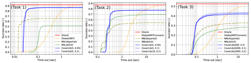
Figure 13: This figure plots the success rate of each planner as a function of the timeout. Note that oracle curve is the upper bound.

VII-A Interpretation of the planning performance comparison (PPC) results

The PPC results in Fig. 5, Fig. 8, and Fig. 11 demonstrate the key advantages of the proposed CoverLib compared to existing approaches. Across all settings, CoverLib achieves higher success rates and substantially higher GPE-TO than NNLibs, indicating that CoverLib-based planning can solve significantly more complex problems. In terms of planning speed, CoverLib is generally as fast as or slightly faster than NNLibs, while providing about an order of magnitude speedup over the Global planner. These results suggest that CoverLib effectively circumvents the plannability-speed trade-off: maintaining the fast planning times of NNLibs while significantly improving the success rate.

It is worth noting that the minimum planning time (the lower tip of the pink line) of CoverLib is generally slightly slower ($\sim$20 ms) than NNLibs. This is because of the cost of $\bar{f}$ evaluation, which involves evaluating $K$ neural networks and generating matrix data (like a heightmap) in $\phi_{\mathrm{emb}}$. Although this difference appears sizable on the logarithmic scale plots, it is not significant in practice considering the speedup over the Global planner. Note that NNLib also incurs the cost of retrieving an experience using nearest neighbor search for a high-dimensional P-space, as evidenced by Fig. 5, even if a Ball Tree is used.

To visualize the plannability-speed trade-off between Global and NNLibs and how CoverLib circumvents it, we plot the timeout-success trade-off curves for the three tasks in Fig. 13. The relationship between Global and NNLibs clearly illustrates the aforementioned trade-off. In contrast, CoverLib significantly circumvents this trade-off, with its curve in closer proximity to the Oracle curves. Here the Oracle refers to a hypothetical planner that can solve any feasible problem instantly, thereby achieving the upper bound of the success rate for all timeouts. The upper bound value is computed as described in Section VI-A.

However, the right side of each plot shows that, given a significant timeout, Global solves more complex problems than CoverLib. Addressing this gap is an obvious avenue for future work and should be pursued by considering the discussion in Section VII-E.

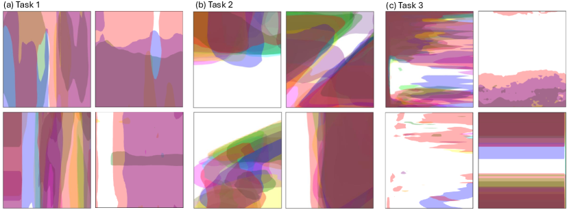
Figure 14: Visualization of classification results of $\hat{f}_{1:K}$ for Tasks 1 to 3. Among $n_{p}$ dimensions, two axes are selected and values for the other dimensions are randomly chosen and fixed. The lower and upper bounds of the axes are set to the minimum and maximum values of the selected dimensions of 1000 samples from $p(\theta)$. The many classified regions lying throughout the boundary of the axes suggest that the adaptation algorithm has a dimensionality reduction nature, and is captured by Coverlib’s classifier. Also, the classified regions often have complex shapes, which are far from those approximated by a sphere or ellipsoid.

VII-B Interpretation of library growth comparison (LGC) results

The LGC plots in Fig.6, Fig.9, and Fig.12 show that while NNLibs demonstrates moderate success rates with small library sizes (e.g., low computational time), its success rate growth is quite slow in the end. In contrast, although CoverLib requires at least a dozen minutes to perform the first iteration (including the CNN pretraining time), it exhibits a significantly faster growth in success rate thereafter, surpassing NNLibs within a couple of hours in all three cases. Despite being unable to investigate further due to our computational time budget, the results suggest that CoverLib’s success rate continues to grow more actively than NNLibs at the end of the experiments. The reason for the increase in the time-per-iteration of CoverLib as the iteration goes on is the adaptable determination of $n_{\mathrm{data}}$ explained in Section IV-C.

However, the LGC plots also suggest that NNLibs is more effective than CoverLib if computational resources are limited, as seen at at the intersection of the LGC curves between CoverLib and NNLibs. However, we must note that the biggest computational bottleneck of CoverLib can be easily parallelized. Considering the trend of more cores in CPUs and the prevalence of cloud computing, the LGC plots of both CoverLib and NNLibs, and hence the intersection of their curves, will likely shift left in the future. This implies that CoverLib will potentially outperform NNLibs in more scenarios in the future.

NNLibs appear to saturate in Tasks 1 and 3, which have high-dimensional P-spaces ($n_{p}=31$ and $n_{p}=87$, respectively), indicating the impact of the curse of dimensionality. In contrast, NNLib(full) still has room for growth in Task 2 with a moderately high-dimensional $n_{p}=10$ P-space, suggesting that the curse of dimensionality is less severe in lower-dimensional spaces. It is noteworthy that NNLib(selected) consistently outperforms NNLib(full) in the high-dimensional Tasks 1 and 3 because feature selection effectively mitigates the curse of dimensionality. However, the observed saturation of NNLib(selected) suggests that the feature selection seems to be less effective in Task 2. This is potentially because the negative effect of ignoring certain dimensions outweighs the positive effect of reducing the dimensionality.

Numerical experiments reveal that $\delta$ greatly impacts CoverLib’s library growth, making the tuning of $\delta$ crucial for CoverLib’s performance. This is because more accurate classifiers are required to achieve the same coverage gain with a smaller $\delta$. However, a larger $\delta$ is not always better. Although not experimentally shown, trivially, setting $\delta$ too large would likely lead to a lower final coverage with early saturation due to overconfidence about coverage. In contrast to $\delta$, the $c_{\mathrm{max}}$ parameter does not seem to significantly affect the library growth. For Tasks 1 and 2, which utilize SQPPlan, this is expected because, beyond a certain number of iterations, the iteration count typically does not impact the solution’s feasibility, although it may influence its optimality. Even in Task 3 using sampling-based ERTConnect, $c_{\mathrm{max}}$ does not significantly affect the library growth rate, as evidenced by the difference between curves $(2000,0.2)$ and $(500,0.2)$ in Fig. 12. A potential explanation is that the coverage gain increase due to a larger $c_{\mathrm{max}}$ is nearly negated by the increased difficulty of fitting $\bar{f}$. As $c_{\mathrm{max}}$ increases, fitting $\bar{f}$ becomes more difficult due to the tail-heavy distribution of $c_{\mathrm{max}}$’s tail extending farther.

VII-C Nonlinear dimensionality reduction nature

CoverLib’s achievement of larger coverage compared to NNLib, despite using a significantly smaller number of experiences, suggests that the “small ball assumption” underlying NNLib, discussed in Section II-A, is invalid. Instead, the adaptation algorithms exhibit a dimensionality reduction nature, which is supported by the visualization of CoverLib’s classifiers in Fig. 14. The figure shows that the classifier’s coverage regions extend throughout the problem distribution in a nonlinear manner, indicating that the effective dimensionality of the P-space for the adaptation algorithms is smaller than $n_{p}$. Note that the min and max values of the axes are set to the minimum and maximum values of the selected dimensions of 1000 samples from $p(\theta)$.

VII-D Note on memory consumption

With the library size of $2^{20}$, NNLib consumes a relatively high amount of memory: 1.1GB, 9.1GB, and 0.9GB for Tasks 1, 2, and 3, respectively. In contrast, CoverLib requires only 114MB, 30MB, and 63MB for the most expensive settings of $(c_{\mathrm{max}},\delta)$ in each task . This significant difference in memory consumption is due to the number of experiences stored. NNLib’s individual experiences consume significantly less memory than CoverLib’s, as they don’t store neural networks. However, NNLib’s much larger number of stored experiences outweighs this difference, resulting in higher overall memory consumption.

VII-E Limitations and future directions

Scalability to inherently complex domains: The numerical experiments demonstrate that even for domains with high-dimensional P-spaces that appear superficially complex, Coverlib can effectively construct a library with high coverage. However, while this suggests that CoverLib scales well with high-dimensional P-spaces, it does not mean scalability with the domain’s inherent complexity. In a case where each dimension introduces a branching factor, the number of experiences required to achieve high coverage will grow exponentially. For example, consider the domain in Fig. 15. Suppose 10 patterns of sub-experiences are needed to handle a single narrow passage, then $10^{4}$ experiences would be required to handle the entire variation of the narrow passages. This is a typical example where CoverLib, or more precisely the library-based method in general, is not expected to remain effective. A similar phenomenon will likely occur to varying degrees when increasing the number of obstacles in Task 1, Task 2, and Task 3. For example, in Task 1, Fig. 4 shows that in successful cases, CoverLib typically found arc- or S-shaped trajectories. However, in cases where CoverLib failed but the global planner succeeded (labeled as “Global success”), the required trajectories appeared more complex. In the Task 1 setup, the number of obstacles was relatively small, making such complex situations rare. However, as the number of obstacles increases, the required trajectories become more diverse, and CoverLib would need a greater variety of experiences to handle these complex situations effectively.

To address this fundamental limitation, vertical composition of experiences could be a promising approach, although this article focuses on horizontal composition. Specifically, a potential solution is to segment the problem into multiple phases and compose the libraries for each phase. Another potential solution is to combine CoverLib with other learning-based methods reviewed in Section II-C. For example, by combining the learned sampling distributions or heuristic maps, the adaptation algorithm can more effectively handle the narrow passages, or just the difficult part in general. For example, in Fig. 15, if we can reduce the number from $10$ to $2$ then the number of experiences required will decrease from $10^{4}$ to $2^{4}$. The same effect can be expected by using a latent space-learning approach.

Training an accurate classifier with small samples: The bottleneck of CoverLib is the dataset generation and neural network training in Step 2. As the iteration progresses, an increasingly accurate classifier is needed to correctly classify the diminishing coverage regions, requiring more data and training time. We needed 1 to 2 days to complete the preprocessing even with extensive parallelization in the above numerical experiments. This hinders us from reaching even closer to the upper bound. To address this limitation, future research could explore two approaches: 1) feature engineering and 2) meta-learning. Pan et al. [41] provide an example of the former approach by defining features as the coupling of trajectory and environment. For the latter approach, meta (cross-domain) learning methods like MAML [42] could be used for pre-training, potentially improving the sample efficiency of training $\bar{f}$.

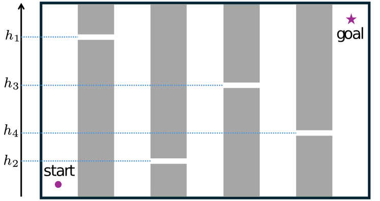
Figure 15: An example domain where the CoverLib method is no longer expected to be effective. The problem instance is a two-dimensional path planning problem with 4 narrow passages, where their positions are parameterized by $\theta=(h_{1},h_{2},h_{3},h_{4})$. Thus the dimension of the P-space is $n_{p}=4$.

VIII Conclusion

This article addresses the plannability-speed trade-off in motion planning methods. Library-based methods offer a promising approach to mitigate this trade-off when the domain of the planning problem is known a priori. We proposed CoverLib, a principled approach that tunes the high-level part of library-based methods to the domain, further alleviating the trade-off.

Numerical experiments demonstrated that CoverLib achieves high plannability (success rate) nearly on par with global planners with high timeouts, outperforming NNLibs in all tasks. Simultaneously, CoverLib’s planning speed surpassed global planners by an order of magnitude by inheriting the speed of library-based methods. The library growth comparison against NNLibs suggested CoverLib’s scalability with high-dimensional problem spaces. Results indicated that NNLibs are prone to the curse of dimensionality of the P-space, while CoverLib is less affected by it. Importantly, the CoverLib method is adaptation-algorithm-agnostic, as demonstrated by the successful integration of both NLP- (in Tasks 1 and 2) and sampling-based (in Task 3) adaptation algorithms.

We hope this work inspires future research not only in motion planning, but also in the broader planning-related community, particularly in the MPC, TAMP and Reinforcement Learning fields.

Hirokazu Ishida received his BE in Aerospace Engineering from Osaka Prefecture University in 2016. He received his MS in Aerospace Engineering from the University of Tokyo in 2018. Since 2019, he has been a Ph.D. student in the Graduate School of Information Science and Technology at the University of Tokyo. His current research interests include the intersection of learning and planning in robotics.

Naoki Hiraoka received BE in Department of Mechano-Informatics from The University of Tokyo in 2019. He received MS in information science and technology from The University of Tokyo in 2021. From 2021, he is a doctoral student in the Graduate School of Information Science and Technology, The University of Tokyo and a Research Fellow of Japan Society for the Promotion of Science. His research interests include whole-body motion planning and control of humanoid robots.

Kei Okada received BE in Computer Science from Kyoto University in 1997. He received MS and PhD in Information Engineering from The University of Tokyo in 1999 and 2002, respectively. From 2002 to 2006, he joined the Professional Programme for Strategic Software Project in The University Tokyo. He was appointed as a lecturer in the Creative Informatics at the University of Tokyo in 2006, an associate professor and a professor in the Department of Mechano-Informatics in 2009 and 2018, respectively. His research interests include humanoids robots, real-time 3D computer vision, and recognition-action integrated system.

Masayuki Inaba graduated from the Department of Mechanical Engineering, University of Tokyo, in 1981, and received MS and PhD degrees from the Graduate School of Information Engineering, University of Tokyo, in 1983 and 1986. He was appointed as a lecturer in the Department of Mechanical Engineering, University of Tokyo, in 1986, an associate professor, in 1989, and a professor in the Department of Mechano-Informatics, in 2000. His research interests include key technologies of robotic systems and software architectures to advance robotics research.

References

- [1] L. E. Kavraki, P. Svestka, J.-C. Latombe, and M. H. Overmars, “Probabilistic roadmaps for path planning in high-dimensional configuration spaces,” IEEE trans. on Robot. and Autom., vol. 12, no. 4, pp. 566–580, 1996.
- [2] S. M. LaValle and J. J. Kuffner Jr, “Randomized kinodynamic planning,” Int. J. Robot. Res., vol. 20, no. 5, pp. 378–400, 2001.
- [3] M. Zucker, N. Ratliff, A. D. Dragan, M. Pivtoraiko, M. Klingensmith, C. M. Dellin, J. A. Bagnell, and S. S. Srinivasa, “Chomp: Covariant hamiltonian optimization for motion planning,” Int. J. Robot. Res., vol. 32, no. 9-10, pp. 1164–1193, 2013.
- [4] J. Schulman, Y. Duan, J. Ho, A. Lee, I. Awwal, H. Bradlow, J. Pan, S. Patil, K. Goldberg, and P. Abbeel, “Motion planning with sequential convex optimization and convex collision checking,” Int. J. Robot. Res., vol. 33, no. 9, pp. 1251–1270, 2014.
- [5] N. Jetchev and M. Toussaint, “Fast motion planning from experience: trajectory prediction for speeding up movement generation,” Auton. Robots, vol. 34, no. 1, pp. 111–127, 2013.
- [6] K. Hauser, “Learning the problem-optimum map: Analysis and application to global optimization in robotics,” IEEE Trans. Robot., vol. 33, no. 1, pp. 141–152, 2016.
- [7] T. S. Lembono, A. Paolillo, E. Pignat, and S. Calinon, “Memory of motion for warm-starting trajectory optimization,” IEEE Robot. Autom. Lett., vol. 5, no. 2, pp. 2594–2601, 2020.
- [8] E. Dantec, R. Budhiraja, A. Roig, T. Lembono, G. Saurel, O. Stasse, P. Fernbach, S. Tonneau, S. Vijayakumar, S. Calinon et al., “Whole body model predictive control with a memory of motion: Experiments on a torque-controlled talos,” in Proc. IEEE Int. Conf. Robot. Autom., 2021, pp. 8202–8208.
- [9] D. Berenson, P. Abbeel, and K. Goldberg, “A robot path planning framework that learns from experience,” in Proc. IEEE Int. Conf. Robot. Autom., 2012, pp. 3671–3678.
- [10] È. Pairet, C. Chamzas, Y. Petillot, and L. E. Kavraki, “Path planning for manipulation using experience-driven random trees,” IEEE Robot. Autom. Lett., vol. 6, no. 2, pp. 3295–3302, 2021.
- [11] F. Islam, O. Salzman, and M. Likhachev, “Provable indefinite-horizon real-time planning for repetitive tasks,” in Proc. Int. Conf. Autom. Plan. Sched., vol. 29, 2019, pp. 716–724.
- [12] F. Islam, O. Salzman, A. Agarwal, and M. Likhachev, “Provably constant-time planning and replanning for real-time grasping objects off a conveyor belt,” Int. J. Robot. Res., vol. 40, no. 12-14, pp. 1370–1384, 2021.
- [13] F. Islam, C. Paxton, C. Eppner, B. Peele, M. Likhachev, and D. Fox, “Alternative paths planner (app) for provably fixed-time manipulation planning in semi-structured environments,” in Proc. IEEE Int. Conf. Robot. Autom., 2021, pp. 6534–6540.
- [14] P. Lehner and A. Albu-Schäffer, “Repetition sampling for efficiently planning similar constrained manipulation tasks,” in Proc. IEEE/RSJ Int. Conf. Intell. Robots. Syst. IEEE, 2017, pp. 2851–2856.
- [15] B. Ichter, J. Harrison, and M. Pavone, “Learning sampling distributions for robot motion planning,” in Proc. IEEE Int. Conf. Robot. Autom., 2018, pp. 7087–7094.
- [16] C. Chamzas, A. Shrivastava, and L. E. Kavraki, “Using local experiences for global motion planning,” in Proc. IEEE Int. Conf. Robot. Autom., 2019, pp. 8606–8612.
- [17] C. Chamzas, A. Cullen, A. Shrivastava, and L. E. Kavraki, “Learning to retrieve relevant experiences for motion planning,” in Proc. IEEE Int. Conf. Robot. Autom., 2022, pp. 7233–7240.
- [18] M. Zucker, J. Kuffner, and J. A. Bagnell, “Adaptive workspace biasing for sampling-based planners,” in Proc. IEEE Int. Conf. Robot. Autom. IEEE, 2008, pp. 3757–3762.
- [19] R. Terasawa, Y. Ariki, T. Narihira, T. Tsuboi, and K. Nagasaka, “3d-cnn based heuristic guided task-space planner for faster motion planning,” in Proc. IEEE Int. Conf. Robot. Autom., 2020, pp. 9548–9554.
- [20] B. Ichter, E. Schmerling, T.-W. E. Lee, and A. Faust, “Learned critical probabilistic roadmaps for robotic motion planning,” in Proc. IEEE Int. Conf. Robot. Autom., 2020, pp. 9535–9541.
- [21] A. H. Qureshi, Y. Miao, A. Simeonov, and M. C. Yip, “Motion planning networks: Bridging the gap between learning-based and classical motion planners,” IEEE Trans. Robot., vol. 37, no. 1, pp. 48–66, 2020.
- [22] T. Ando, H. Iino, H. Mori, R. Torishima, K. Takahashi, S. Yamaguchi, D. Okanohara, and T. Ogata, “Learning-based collision-free planning on arbitrary optimization criteria in the latent space through cgans,” Adv. Robot., vol. 37, no. 10, pp. 621–633, 2023.
- [23] B. Ichter and M. Pavone, “Robot motion planning in learned latent spaces,” IEEE Robot. Autom. Lett., vol. 4, no. 3, pp. 2407–2414, 2019.
- [24] D. Coleman, I. A. Şucan, M. Moll, K. Okada, and N. Correll, “Experience-based planning with sparse roadmap spanners,” in Proc. IEEE Int. Conf. Robot. Autom., 2015, pp. 900–905.
- [25] C. R. Garrett, R. Chitnis, R. Holladay, B. Kim, T. Silver, L. P. Kaelbling, and T. Lozano-Pérez, “Integrated task and motion planning,” Annu. Rev. Control, Robot., Auton. Syst., vol. 4, pp. 265–293, 2021.
- [26] G. L. Nemhauser, L. A. Wolsey, and M. L. Fisher, “An analysis of approximations for maximizing submodular set functions―i,” Math. program., vol. 14, pp. 265–294, 1978.
- [27] A. Krause and D. Golovin, “Submodular function maximization.” Tractability, vol. 3, no. 71-104, p. 3, 2014.
- [28] N. Hansen, S. D. Müller, and P. Koumoutsakos, “Reducing the time complexity of the derandomized evolution strategy with covariance matrix adaptation (cma-es),” Evol. Comput., vol. 11, no. 1, pp. 1–18, 2003.
- [29] M. Nomura and M. Shibata, “cmaes: A simple yet practical python library for cma-es,” arXiv preprint arXiv:2402.01373, 2024.
- [30] S. M. Omohundro, Five balltree construction algorithms. International Computer Science Institute Berkeley, 1989.
- [31] B. Stellato, G. Banjac, P. Goulart, A. Bemporad, and S. Boyd, “Osqp: An operator splitting solver for quadratic programs,” Math. Program. Comput., vol. 12, no. 4, pp. 637–672, 2020.
- [32] P. Virtanen, R. Gommers, T. E. Oliphant, M. Haberland, T. Reddy, D. Cournapeau, E. Burovski, P. Peterson, W. Weckesser, J. Bright et al., “Scipy 1.0: fundamental algorithms for scientific computing in python,” Nature methods, vol. 17, no. 3, pp. 261–272, 2020.
- [33] R. Tedrake, “Underactuated robotics: Learning, planning, and control for efficient and agile machines course notes for mit 6.832,” Working draft edition, vol. 3, no. 4, p. 2, 2009.
- [34] L. Janson, E. Schmerling, A. Clark, and M. Pavone, “Fast marching tree: A fast marching sampling-based method for optimal motion planning in many dimensions,” Int. J. Robot. Res., vol. 34, no. 7, pp. 883–921, 2015.
- [35] D. J. Webb and J. Van Den Berg, “Kinodynamic rrt*: Asymptotically optimal motion planning for robots with linear dynamics,” in Proc. IEEE Int. Conf. Robot. Autom., 2013, pp. 5054–5061.
- [36] K. Kojima, T. Karasawa, T. Kozuki, E. Kuroiwa, S. Yukizaki, S. Iwaishi, T. Ishikawa, R. Koyama, S. Noda, F. Sugai et al., “Development of life-sized high-power humanoid robot jaxon for real-world use,” in Proc. IEEE-RAS Int. Conf. Humanoid Robots., 2015, pp. 838–843.
- [37] D. Kappler, F. Meier, J. Issac, J. Mainprice, C. G. Cifuentes, M. Wüthrich, V. Berenz, S. Schaal, N. Ratliff, and J. Bohg, “Real-time perception meets reactive motion generation,” IEEE Robot. Autom. Lett., vol. 3, no. 3, pp. 1864–1871, 2018.
- [38] Z. Kingston, M. Moll, and L. E. Kavraki, “Sampling-based methods for motion planning with constraints,” Annu. Rev. Control, Robot., Auton. Syst., vol. 1, pp. 159–185, 2018.
- [39] N. Hiraoka, H. Ishida, T. Hiraoka, K. Kojima, K. Okada, and M. Inaba, “Sampling-based global path planning using convex polytope approximation for narrow collision-free space of humanoid,” Int. J. of Humanoid Robot., 2024, in press and available online.
- [40] I. A. Sucan, M. Moll, and L. E. Kavraki, “The open motion planning library,” IEEE Robot. Autom. Mag., vol. 19, no. 4, pp. 72–82, 2012.
- [41] J. Pan, Z. Chen, and P. Abbeel, “Predicting initialization effectiveness for trajectory optimization,” in Proc. Int. Conf. Robot. Autom. IEEE, 2014, pp. 5183–5190.
- [42] C. Finn, P. Abbeel, and S. Levine, “Model-agnostic meta-learning for fast adaptation of deep networks,” in Proc. Int. Conf. Mach. Learn. PMLR, 2017, pp. 1126–1135.
- [43] I. Goodfellow, Y. Bengio, and A. Courville, Deep learning. MIT press, 2016.
- [44] A. Paszke, S. Gross, F. Massa, A. Lerer, J. Bradbury, G. Chanan, T. Killeen, Z. Lin, N. Gimelshein, L. Antiga et al., “Pytorch: An imperative style, high-performance deep learning library,” Proc. Adv. Neural Inf. Process. Syst., vol. 32, 2019.