Trade-off relations between Bell nonlocality and local Kochen-Specker contextuality in generalized Bell scenarios

Abstract

The relations between Bell nonlocality and Kochen-Specker contextuality have been subject of research from many different perspectives in the last decades. Recently, some interesting results on these relations have been explored in the so-called generalized Bell scenarios, that is, scenarios where Bell spatial separation (or agency independence) coexist with (at least one of the) parties’ ability to perform compatible measurements at each round of the experiment. When this party has an $n$-cycle compatiblity setup, it was first claimed that Bell nonlocality could not be concomitantly observed with contextuality at this party’s local experiment. However, by a more natural reading of the definition of locality, it turns out that both Bell nonlocality and local contextuality can, in fact, be jointly present. In spite of it, in this work we prove that there cannot be arbitrary amounts of both of these two resources together. That is, we show the existence of a trade-off relation between Bell nonlocality and local contextuality in such scenarios. We explore this trade-off both in terms of inequalities and quantifiers, and we discuss how it can be understood in terms of a ‘global’ notion of contextuality. Furthermore, we show that such notion does not only encompass local contextuality and Bell nonlocality, but also other forms of nonclassical correlations.

I Introduction

Bell nonlocality [1, 2] and Kochen-Specker contextuality [3, 4] are two of the most remarkable features of quantum theory. They reveal a fundamental contrast between its predictions and those of classical theories. As such, they constitute some of the cornerstones for how our current understanding of quantum theory is conceived. They are also essential resources for quantum advantage in informational tasks.

Nonlocality and contextuality are in fact closely related concepts, since they both are associated to stronger-than-classical correlations between the outcomes of compatible measurements. Bell nonlocality can actually be seen as a particular case of contextuality, which takes place in scenarios where there exist multiple observers far apart (or informationally isolated) from each other and the compatibility relations are solely inherited from such spatial separation.

The similarity between these two concepts motivates investigations from many different perspectives to better understand their connections. For example, since the first decades after they were discovered, there is an ongoing search for how to convert proofs of contextuality into proofs of nonlocality [5, 6, 7, 8]. In another direction, the Cabello-Severini-Winter graph-theoretic approach [9, 10] can be adapted to demand compatibilities coming from separated parties [11], allowing one to compare the sets of quantum correlations coming from Bell or Bell-like scenarios with the larger quantum sets allowed in contextuality scenarios [12, 13].

In yet another way, the relations between nonlocality and contextuality can be explored in the framework of the so-called generalized Bell scenarios [14, 15]. These are Bell scenarios where (at least) one of the parties is allowed to perform compatible measurements on their local system at each round of the experiment. This party is then able to make a local contextuality test at the same time as the nonlocality experiment is performed amongst all the observers [16]. These are precisely the scenarios we study in this work.

In recent years, some rather surprising results on the simplest generalized Bell scenarios have been explored in literature. For example, in the bipartite scenario where Alice has two incompatible measurements and Bob has a $5$-cycle setup [17], local contextuality on Bob’s experiment has been observed concomitantly with Bell nonlocal correlations between him and Alice [16], a phenomenon that was previously thought to be impossible [15, 18]. The key fact behind this joint observation is a suitable modification in the definition of Bell nonlocality, specifically tailored for the generalized scenarios [19, 14]. This new definition is in fact more powerful than the usual one, and leads to new relevant classes of Bell-like inequalities. One of these new inequalities, in particular, is then used to jointly witness nonlocality and contextuality in the above mentioned scenario [16].

In this work, we further investigate the relations between these different types of nonclassicalities in generalized Bell scenarios. More specifically, we prove that even though nonlocality and contextuality can be jointly observed in scenarios such as the one mentioned above, they still satisfy trade-off relations. That is, there cannot be arbitrary amounts of both nonlocality and contextuality together. Moreover, we extend our arguments to go beyond the scenarios where Bob has an $n$-cycle setup, by identifying geometrical conditions that lead to such a trade-off. Finally, after defining quantifiers of nonlocality and contextuality for generalized Bell scenarios and rephrasing the trade-off relations in terms of them, we explore a more general notion of nonclassical correlations that may appear in these scenarios.

The manuscript is structured as follows. In Section II, we discuss some of the background required and introduce the concepts related to generalized Bell scenarios. In Section III, we show that in the generalized Bell scenarios where Bob has an $n$-cycle, maximal contextuality on his experiment implies locality in the generalized scenario. On the other hand, we also show that, for small values of $n$, maximal nonlocality implies noncontextuality on Bob’s experiment. In section IV we discuss which are the features of these scenarios that lead to such a relation. Then, we explore the consequences of the trade-off in terms of inequalities, and in terms of quantifiers in Section V and Section VI, respectively. We conclude in Section VII, also discussing some of the further questions raised by this work.

II Preliminaries

In this section, we present some of the definitions and previous results relevant to our discussion. In particular, we introduce the generalized Bell scenarios and discuss some of the distinct definitions of locality applicable to them [19, 14]. Also, we present some of the recent results relating nonlocality and local contextuality on these scenarios.

II.1 Contextuality and polytopes

To begin with, let us recall some of the basic concepts related to Kochen-Specker contextuality [4]. A contextuality scenario is specified by a set of measurements $\mathcal{M}$, their compatibility relations, and a set of possible outcomes for each of them $\mathcal{O}$. The compatibility relations are typically specified by a set $\mathcal{C}$, whose elements are subsets of $\mathcal{M}$ composed by compatible observables. The elements of $\mathcal{C}$, that is, the sets of measurements which can be jointly performed, are named contexts.

Then, to describe a contextuality experiment we need, for each context $C\in\mathcal{C}$, a probability distribution $p_{C}$ for its possible outcomes. These probabilities, considering all contexts and all possible outcomes, can be organized as the entries of a vector $\bm{p}\in\mathbb{R}^{d}$ in an appropriate dimension $d$. This vector is called behavior of the experiment.

The acceptable behaviors in a contextuality scenario are typically required to satisfy some consistency conditions, known as no-disturbance conditions, stating that marginals be well defined. More specifically, for every $C,C^{\prime}\in\mathcal{C}$, these conditions can be written as

$$p_{C|C\cap C^{\prime}}=p_{C^{\prime}|C\cap C^{\prime}},$$ (1)

where $p_{C|C\cap C^{\prime}}$ denotes the restriction of the distribution $p_{C}$ to the measurements in the intersection $C\cap C^{\prime}$.

A behavior is said to be noncontextual if there exists a variable $\lambda$, described by a probability distribution $q(\lambda)$, such that for every $C\in\mathcal{C}$ we can write

$$p_{C}(\bm{s})=\sum_{\lambda}q(\lambda)\prod_{M\in C}p_{M}^{\lambda}(s_{M}),$$ (2)

where $\bm{s}$ denotes the outcome of the context $C$, and $s_{M}$ denotes the corresponding outcome of the measurement $M\in C$. Moreover, $p_{M}^{\lambda}$ is a probability distribution on the outcomes of the measurement $M$ which may depend on $\lambda$.

Fine’s theorem states that the distributions $p^{\lambda}_{M}$ might be taken to be deterministic without loss of generality [20]. Thus, the noncontextual behaviors are convex combinations of deterministic behaviors, that is, behaviors whose entries are either $0$ or $1$, respecting the no-disturbance conditions. So, in a noncontextual behavior it is possible to think of measurements as if they were simply revealing a property of the system which was already well defined prior to the measurements. In this case, the probabilities only arise as a consequence of a lack of knowledge of the system’s preparation, in accordance with what we would expect within a classical theory.

Geometrically, both the set of nondisturbing behaviors and the set of noncontextual behaviors in $\mathbb{R}^{d}$ are polytopes. A polytope is a bounded convex set specified by a finite number of linear inequalities. Every polytope has a finite set of points which cannot be written as a convex combination of any other points belonging to it, the so-called vertices, or extremal points of the polytope. A polytope can also be alternatively defined as the convex hull of such points. In fact, there is a fundamental result in polyhedral theory, known as Minkowski’s theorem, stating the equivalence between these two descriptions of a polytope, either in terms of inequalities or in terms of its vertices [21].

Even though one could, in principle, interchange between the two descriptions of polytopes, this is, in general, a difficult task. There are computational methods, such as the one described in [22], which can handle this transformation for sufficiently simple cases. Nevertheless, these methods do not scale particularly well with the dimension of the polytope [22].

In a typical contextuality scenario, we easily know how to specify the noncontextual polytope by its vertices, which are the deterministic behaviors. However, for many reasons it is desirable to characterize it in terms of inequalities, often called noncontextuality inequalities. Beyond the computational tools mentioned in the last paragraph, there are some scenarios, such as the $n$-cycles, where the inequalities characterizing the noncontextual polytope have been analytically found [17].

On the other hand, we easily know how to specify the nondisturbing polytope via the inequality description, using no-disturbance conditions and non-negativity and normalization of probabilities. For some of the purposes of this work, however, it will be useful to characterize it via the vertex description. Again, in some scenarios, e.g., the $n$-cycles, we can find these vertices analytically [17]. In cases considered in this manuscript, though, we will resort to the computational methods previously mentioned (see Section III)[22].

II.2 Usual and generalized Bell scenarios

So far, the discussion concerns arbitrary contextuality scenarios. Now, to include the notion of nonlocality, we must consider scenarios of a particular kind, namely, those composed by multiple observers spatially separated from one another. For simplicity, we only consider scenarios composed of two parties, referred to as Alice and Bob.

Usually, to define a Bell scenario we specify the number of measurements each of the parties can perform on her respective subsystem, as well as the number of possible outcomes per measurement. Then, in a typical Bell experiment, Alice and Bob each receive a part of jointly prepared physical system, and then each of the parties independently choose one measurement to be performed on their individual system. Denoting Alice’s measurement choice by $x$, and Bob’s by $y$, we might describe such a Bell experiment by probability distributions $p_{xy}$ on the possible outcomes of $x$ and $y$. Repeating the experiment many times, Alice and Bob are able to estimate such probabilities.

Notice that a Bell scenario nicely falls into the description of a contextuality scenario. In this case, the contexts are given by a pair $xy$ composed of one measurement of Alice and one measurement of Bob. That is, the compatibility relations are granted by the spatial separation between the observers. Then, the no-disturbance conditions (1) lead to the so-called no-signaling conditions, which state that the probability distribution describing Alice’s (Bob’s) local experiment does not depend on Bob’s (Alice’s) measurement choice.

The noncontexutal behaviors of a Bell scenario are named local behaviors, and they satisfy

$$p_{xy}(a,b)=\sum_{\lambda}q(\lambda)p_{x}^{\lambda}(a)p_{y}^{\lambda}(b),$$ (3)

where $a$ ($b$) denotes the possible outcomes of the measurement $x$ ($y$), while $q(\lambda)\geq 0$ and $\sum_{\lambda}q(\lambda)=1$ here and in every subsequent use of this notation.

On the other hand, in the so-called a generalized Bell scenario, instead of only performing one measurement at each round of the experiment, Alice and/or Bob are allowed to jointly perform compatible measurements on their local systems. For simplicity, we restrict the discussion to scenarios where Alice still performs one measurement at each round, and only Bob has compatible measurements. Thus, in a generalized Bell scenario of this kind, a behavior is given by probability distributions $p_{x,C_{B}}$, where $x$ denotes Alice’s single measurement and $C_{B}$ denotes a context of Bob’s experiment, i.e., a set of compatible measurements he is able to perform.

A generalized Bell scenario also can be seen as a contextuality scenario according to our previous discussion. In this case, the no-disturbance conditions represent both no-signaling conditions and no-disturbance conditions on Bob’s local experiment. Thus, we refer to the set of acceptable behaviors in generalized Bell scenarios as $\mathcal{NSND}$ (nonsignaling and nondisturbing) polytope.

For the sake of nomenclature, when dealing with the whole scenario as a single contextuality setup, we will refer to noncontextual behaviors as classical behaviors. Thus, classical behaviors are convex combinations of nonsignaling and nondisturbing deterministic ones. Or, equivalently, a behavior $p_{x,C_{B}}$ is said to be classical if it admits a decomposition of the form

$$p_{x,C_{B}}(a,\bm{b})=\sum_{\lambda}q(\lambda)p_{x}^{\lambda}(a)\prod_{M\in C_{B}}p_{M}^{\lambda}(b_{M}),$$ (4)

where $\bm{b}$ denotes the outcome of Bob’s context $C_{B}$, and $b_{M}$ denotes the corresponding outcome of measurement $M\in C_{B}$.

From now on, in the generalized Bell scenarios here considered the term ‘contextuality’ will be used in reference to local contextuality on Bob’s marginal experiment. That is, a behavior of the generalized scenario will be said to be noncontextual if Bob’s marginal is noncontextual.

We should also be careful with the notions of locality for the generalized Bell scenarios. To begin with, notice that the definition (3) can also be applied to such scenarios. To do so, however, we cannot consider the full behavior $p_{x,C_{B}}$ at once. Rather, we should marginalize it to consider only one measurement $y$ of Bob at a time. We will refer to this as the usual notion of locality.

Nevertheless, since Bob is typically performing more than one measurement at each round of the experiment, there might be correlations between Alice and a whole context of Bob. In this sense, in Ref. [19] the authors propose a generalized definition of locality, given by

$$p_{x,C_{B}}(a,\bm{b})=\sum_{\lambda}q(\lambda)p_{x}^{\lambda}(a)p_{C_{B}}^{\lambda}(\bm{b}),$$ (5)

where $\bm{b}$ denotes a possible (joint) outcome for the context $C_{B}$. Here, we ask for $p_{C_{B}}^{\lambda}$ to be only a nondisturbing behavior of Bob’s setup, and this is the key difference when this definition is compared with equation (4), where the response functions of Bob’s are also required to be noncontextual [14]. Furthermore, notice that if a behavior is local according to the generalized definition (5), it is also local in the usual sense, given by equation (3), considering any of the appropriate marginalizations.

Let us also stress that the generalized definition of locality is better suited to the generalized scenarios than the usual one, as it takes the local compatibility structure of Bob into account. This will be the main notion of locality adopted in this work, and it is to be understood that whenever we mention ‘locality’ in a generalized Bell scenario, we are referring to the generalized definition. Moreover, the inequalities associated with this definition of locality will be referred to as generalized Bell inequalities.

Geometrically, in the generalized scenarios the visualization of the sets of interest is somewhat more complicated than in a typical contextuality scenario, or even in an usual Bell scenario, see Figure 1. Note that the $\mathcal{NSND}$ polytope contains (but is not necesserily equal to) the set all physically acceptable behaviors for the generalized scenario. Entirely contained in it, the classical polytope is the convex hull of the deterministic behaviors. The noncontextual polytope has nonempty intersection with the classical polytope, but there are also noncontextual behaviors that are nonclassical, since they may be nonlocal. Furthermore, there are the usual-local and generalized-local polytopes, the latter contained in the former and none entirely contained in the classical polytope, since both have contextual points. Finally, it will be important to consider the nondisturbing polytope of Bob’s marginal experiment, which can be seen as a projection of the $\mathcal{NSND}$ polytope of the whole scenario.

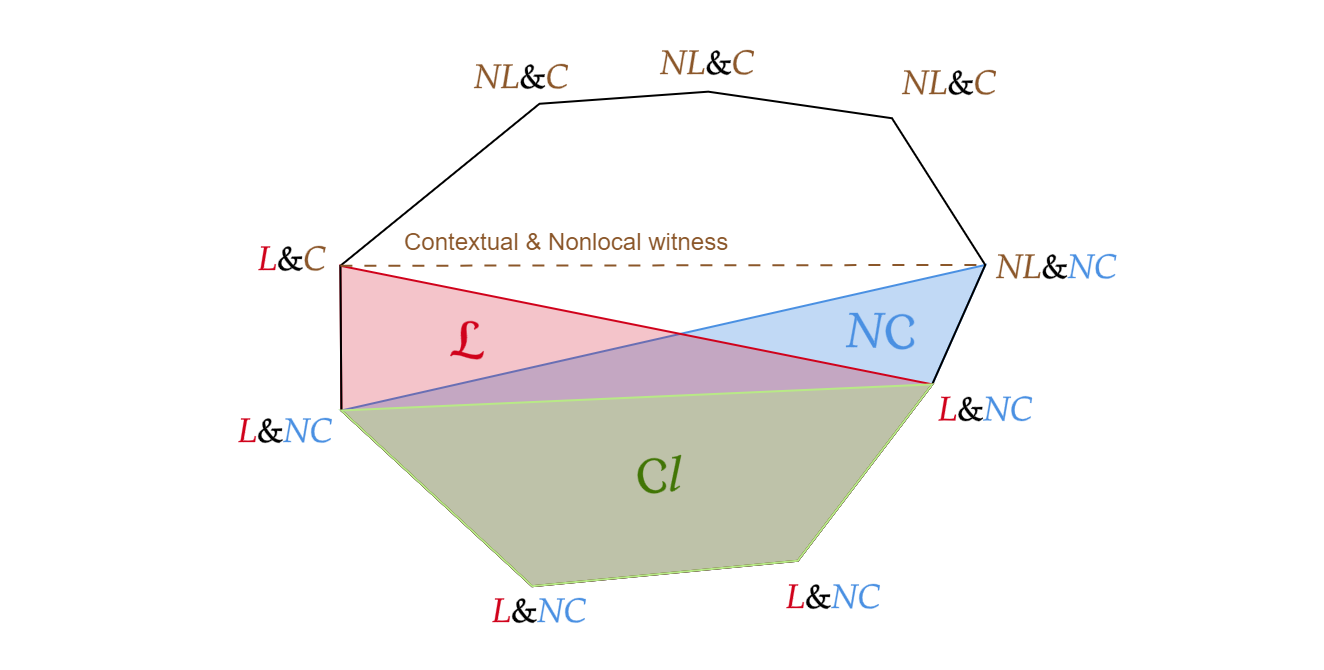
Figure 1: Schematic figure representing the $\mathcal{NSND}$ polytope of a generalized Bell scenario, highlighting all its possible kinds of vertices and interesting subpolytopes it contains. There can be local and noncontextual vertices, whose convex hull constitutes the classical ($\mathcal{C}l$) polytope (green region); there can also be local and contextual vertices, which, together with the local and noncontextual vertices, are the vertices of the local ($\mathcal{L}$) (union of the green and the red regions); there are nonlocal and noncontextual vertices, which are also vertices of the noncontextual ($\mathcal{NC}$) polytope (union of the green and the blue regions); and finally there can be nonlocal and contextual vertices. Also depicted in the figure is a joint witness of nonlocality and contextuality, i. e., an inequality that can only be violated by behaviors which are nonlocal and contextual at the same time.

II.3 Relations between nonlocality and contextuality in generalized Bell scenarios

Let us now move on to the discussion of some of the recent results relating nonlocality and contextuality in generalized Bell scenarios. Most of them have to do with a particular kind of the scenarios we discussed in the previous section, where the contextuality setup of Bob is an $n$-cycle [17]. That is, Bob is able to perform $n$ possible measurements $\{B_{0},B_{1},...,B_{n-1}\}$, with contexts $\{B_{i},B_{i+1}\}$ (sum modulo $n$). All the measurements $B_{i}$, as well as Alice’s measurements, that from now on will be denotet by $A_{x}$, with $x=0,1$, are dichotomic, with outcomes labeled by $+1$ and $-1$.

One of the reasons why an $n$-cycle contextuality scenario is interesting is the fact that the nondisturbing polytope has been completely characterized in terms of its vertices, and the noncontextual polytope has been completely characterized in terms of its inequalities. Moreover, the $5$-cycle corresponds to the KCBS scenario [23], which is the simplest scenario for which quantum theory exhibits contextuality. These generalized scenarios, where Alice has two incompatible measurements and Bob has an $n$-cycle setup, are also the focus of this work.

In Ref. [15], the authors consider precisely the scenario in which Bob has a KCBS setup. Then, they analyze violations of a KCBS inequality on Bob’s experiment,

$$\begin{split}\beta_{KCBS}=\langle B_{0}B_{1}\rangle+\langle B_{1}B_{2}\rangle+\langle B_{2}B_{3}\rangle\\ +\langle B_{3}B_{4}\rangle-\langle B_{4}B_{0}\rangle\leq 3,\end{split}$$ (6)

together with a CHSH inequality of the form

$$\alpha_{CHSH}=\langle A_{0}B_{i}\rangle+\langle A_{0}B_{j}\rangle+\langle A_{1}B_{i}\rangle-\langle A_{1}B_{j}\rangle\leq 2,$$ (7)

where $B_{i}$ and $B_{j}$ are incompatible measurements of Bob. Notice that this CHSH inequality is associated with the usual notion of locality.

Using the techniques of Ref. [24], it is possible to prove that for every nondisturbing behavior of the generalized scenario, the following relation holds:

$$\alpha_{CHSH}+\beta_{KCBS}\leq 5.$$ (8)

In other words, inequalities (6) and (7) cannot be simultaneously violated in such an experiment [15].

Furthermore, notice that all the Bell inequalities associated with the usual notion of locality in such a scenario are CHSH inequalities of the form (7), up to relabelings [25]. Also, all the noncontextuality inequalities for Bob’s experiment are known, and are also similar to (6) up to relabelings.

The argument leading to equation (8) can then be applied to any of those CHSH inequalities together with any of the noncontextuality inequalities of the scenario. Therefore, if Alice and Bob share nonlocal correlations (according to the usual sense of locality), then Bob’s local experiment cannot exhibit contextuality. Conversely, if Bob’s experiment exhibits contextuality, then the correlations with Alice are local. That is, there is a fundamental monogamy relation between contextuality and the usual notion of locality in this scenario. The same argument was later extended to scenarios where Bob can perform joint measurements according to an arbitrary $n$-cycle [18].

However, as we discussed in the previous section, the usual definition of locality, the one considered to prove this monogamy, is not the most appropriate notion of locality for generalized Bell scenarios. Thus, it is intersting to investigate whether this monogamy still holds when considering the generalized definition of locality proposed in Ref. [19].

In Ref. [16], the authors present a negative answer to this question. They show a family of quantum states exhibiting both local contextuality on Bob’s experiment and nonlocality in the generalized sense. The conclusion, then, is that there is not a strict monogamy relation between contextuality and nonlocality when the adequate definitions are considered.

Nevertheless, such results suggest that there would still exist a certain trade-off between nonlocality and contextuality in such scenarios. This phenomenon can be clearly seen for a particular pair of Bell and noncontextuality inequalities investigated in Ref [16]. It was, however, unclear whether this trade-off relation was a particularity of the inequalities considered, or if this relation was a fundamental feature of these scenarios. That is the question we investigate in this manuscript.

III A first glance at the trade-off: the cycle scenarios

In this section, we analyze the suggested trade-off between nonlocality and contextuality when considering nonsignaling and nondisturbing behaviors in the scenarios where Bob has an $n$-cycle. For that matter, we start investigating behaviors which exhibit ‘maximal’ contextuality or ‘maximal’ nonlocality: behaviors whose violation of a noncontextuality or generalized-Bell inequality, respectively, is the maximum allowed within the $\mathcal{NSND}$ polytope.

Result 1

Consider a generalized bipartite Bell scenario where Alice has two incompatible measurements and Bob has an $n$-cycle contextuality setup. If a $\mathcal{NSND}$ behavior maximally violates a noncontextuality inequality of Bob’s marginal experiment, then it must be local.

Proof: To prove this statement, we start by showing that, in an $n$-cycle contextuality scenario, the only behaviors which maximally violate noncontextuality inequalities are vertices of the associated nondisturbing polytope. To do so, let us recall that the contextual vertices of the nondisturbing polytope of such scenarios are given by:

$$\langle B_{i}\rangle=0$$ (9a)

$$\langle B_{i}B_{i+1}\rangle=\gamma_{i},$$ (9b)

where $i=1,2,...,n$ and $\gamma_{i}=\pm 1$, such that the number of $i$’s for which $\gamma_{i}=-1$ is odd [17].

Now, consider a generic noncontextuality inequality of an $n$-cycle scenario. Since the inequality is linear, there must be at least one vertex of the $\mathcal{NSND}$ polytope which maximally violates it. If there are two such vertices, then all convex combinations of them would also violate it maximally and, thus, be maximally contextual. However, an equally weighted convex combination of any two distinct such vertices is proven to be noncontextual [26]. Thus, there can only be one vertex which maximally violates this inequality, and it also follows that this is the only behavior achieving this violation.

To complete the proof, we slightly modify an argument presented in Ref. [27] to the generalized scenarios. Consider a behavior $p_{A_{x},B_{i}B_{i+1}}$ such that Bob’s marginal $p_{B_{i}B_{i+1}}$ is a vertex of his nondisturbing polytope. Then, we may write

$$\begin{split}p_{B_{i}B_{i+1}}(b_{i},b_{i+1})=\sum_{a}p_{A_{x},B_{i}B_{i+1}}(a,b_{i},b_{i+1})\\ =\sum_{a}p_{A_{x}}(a)\ p^{A_{x}}_{B_{i}B_{i+1}}(b_{i},b_{i+1}|a).\end{split}$$ (10)

Notice that, for each value of $a$, $p^{A_{x}}_{B_{i}B_{i+1}}(b_{i},b_{i+1}|a)$ can be seen as a nondisturbing behavior of Bob’s local experiment, and the above sum is a convex combination of such behaviors. However, since $p_{B_{i}B_{i+1}}$ is a vertex of Bob’s nondisturbing polytope, then the above convex combination must be composed of only one term. That is, $p_{A_{x},B_{i}B_{i+1}}(a,b_{i},b_{i+1})=p_{A_{x}}(a)p_{B_{i}B_{i+1}}(b_{i},b_{i+1})$ and there is no correlation whatsoever between Alice and Bob.  

Thus, in the scenarios here considered, this result shows that if a behavior is maximally contextual, it cannot contain the tiniest amount of nonlocality, it has to be local. Moreover, Alice and Bob are completely uncorrelated.

On the other hand, let us now explore whether the same kind of phenomenon happens for maximally nonlocal behaviors, that is, whether a maximally nonlocal behavior can be contextual. Analytically, this is a much harder question to address, since it genuinely involves the geometry of the whole $\mathcal{NSND}$ polytope. A significant part of the proof of Result 1 is based on the nondisturbing polytope of Bob’s local experiment, which is a much simpler and well-known set. Still, for (at least) a few simple scenarios, this question might be addressed with the aid of computational methods.

Result 2

Consider a generalized bipartite Bell scenario where Alice has two incompatible measurements and Bob has an $n$-cycle contextuality setup, with $n=3$, $4$ or $5$. If an $\mathcal{NSND}$ behavior maximally violates a generalized-Bell inequality, then Bob’s marginal must be noncontextual.

Proof: As previously discussed, there is a duality in the description of a polytope: one might describe it either in terms of linear inqualities, or in terms of its vertices. We know how to specify the $\mathcal{NSND}$ polytope using inequalities, and based on this we can use computational tools to obtain its vertex description [22]. The code details and the list of vertices for the three scenarios $n=3$, $4$ and $5$ are available at [28].

Once all the vertices of the $\mathcal{NSND}$ polytope are enumerated, it is possible to identify the local and the nonlocal ones. The local vertices, for instance, are easily identifiable, because, in this case, Alice’s marginal behavior must be deterministic. All the other vertices are nonlocal. Then, for the nonlocal vertices, the values of all the noncontextuality inequalities’ expressions, which are known for $n$-cycle scenarios [17], are computed. If all inequalities are satisfied, we conclude that the behavior is noncontextual. The result then follows from the fact that all nonlocal vertices of the $\mathcal{NSND}$ polytope for the considered scenarios are noncontextual, and if a behavior maximally violates a generalized-Bell inequality, then it must either be one of such nonlocal vertices, or a convex combination of them.  

So, at least in the simplest of the scenarios we consider, maximal nonlocality implies noncontextuality. In fact, we believe this remains true for every $n$-cycle setup of Bob.

Conjecture 1

In any generalized bipartite Bell scenario where Alice has two incompatible measurements and Bob has an $n$-cycle setup, if an $\mathcal{NSND}$ behavior maximally violates a generalized-Bell inequality, then Bob’s marginal must be noncontextual.

This conjecture is mostly based on the fact that the $n$-cycle contextuality scenarios are very similar to one another. Notice, for instance, that for all $n$, both the vertices of the nondisturbing polytope and noncontextuality inequalities have similar forms [17]. In addition, this similarity seems to be carried out to the generalized scenarios. For example, the strict monogamy relation (8) and the synchronous observation of nonlocality and contextuality reported in Ref. [16] are seen in generalized scenarios where Bob has an arbitrary $n$-cycle setup.

To reinforce the conjecture, in the appendices we present results for specific families of generalized Bell inequalities valid for scenarios were Bob has an $n$-cycle setup. We show, for instance, that maximal violations of such inequalities imply noncontextuality. In Appendix A, we consider CHSH-like inequalities [30, 19, 16], and in Appendix B we deal with generalizations of the so-called chained inequalities [31, 32].

IV Which scenarios exhibit this trade-off?

At this point, we have proven that in the scenarios where Bob has an $n$-cycle, all maximally contextual behaviors are local, and conjectured that all maximally nonlocal behaviors are noncontextual, a fact which was verified for particular values of $n$. However, before we explore the consequences of this relation between nonlocality and contextuality, we first discuss the features of such scenarios which are responsible for this relation. In other words, we analyze which conditions must be met in generalized Bell scenarios so that all maximally nonlocal behaviors are noncontextual and all maximally contextual behaviors are local.

To begin with, notice that the key fact to prove Result 2 for the simplest cycle scenarios is that all nonlocal vertices of their $\mathcal{NSND}$ polytopes are noncontextual. This is equivalent to saying that all maximally nonlocal behaviors are noncontextual. It turns out that this fact also implies that all maximally contextual behaviors are local, as we prove in the following.

For the sake of clarity, if a generalized Bell scenario where only Bob has compatible measurements is such that all the nonlocal vertices of its $\mathcal{NSND}$ polytope are noncontextual, we say that this scenario only has monogamous vertices.

Lemma 1

In a bipartite generalized Bell scenario where only Bob has compatible measurements, all the maximally nonlocal behaviors are noncontextual and all the maximally contextual behaviors are local if, and only if, this scenario only has monogamous vertices.

Proof: In a given generalized Bell scenario, it is not difficult to see that all maximally nonlocal behaviors are noncontextual if and only if the scenario only contains monogamous vertices, as we mentioned in the proof of Result 2. So, for this lemma to be proved, we only need to prove that if the scenario only contains monogamous vertices, then all maximally contextual behaviors are local. Consider a behavior of the generalized scenario such that Bob’s marginal behavior maximally violates a noncontextuality inequality. Then, any decomposition of Bob’s marginal behavior in terms of the vertices of its $\mathcal{ND}$ polytope can only include contextual vertices. Thus, any decomposition of the behavior of the generalized scenario can also only include contextual vertices of the associated $\mathcal{NSND}$ polytope. However, by hypotesis, all of those vertices are local.  

In summary, if we want to verify whether a generalized Bell scenario exhibits the trade-off relation between nonlocality and contextuality just described, we need to analyze the vertices of its $\mathcal{NSND}$ polytope. If the scenario only contains monogamous vertices, then the trade-off holds. Otherwise, at least one of the following is true: either there exists a behavior which maximally violates a generalized-Bell inequality and is, at the same time, contextual, or there exists a behavior which maximally violates a noncontextuality inequality and is, at the same time, nonlocal.

However, as we have mentioned, enumerating the $\mathcal{NSND}$ vertices of a generalized Bell scenario is, usually, a difficult task. So, it is useful to have other means to conclude that a scenario only contains monogamous vertices. For example, the following lemma states sufficient conditions for that to happen.

Lemma 2

Consider a bipartite generalized Bell scenario where only Bob has compatible measurements and such that the following properties hold:

(i) every contextual vertex of the $\mathcal{NSND}$ polytope of the generalized scenario is such that Bob’s marginal maximally violates a noncontextuality inequality; and

(ii) Bob’s local contextuality scenario is such that the only behaviors which maximally violate noncontextuality inequalities are vertices of its nondisturbing polytope.

Then, the $\mathcal{NSND}$ polytope of this scenario only has monogamous vertices.

Proof: The two conditions allow us to conclude that all contextual vertices of the $\mathcal{NSND}$ polytope are such that Bob’s marginals are vertices of his $\mathcal{ND}$ polytope. Then, analogously to the proof of Result 1, we conclude that every contextual vertex is local, that is, the scenario only contains monogamous vertices.  

For the scenarios where Bob has an $n$-cycle setup, discussed in the previous section, we can prove that condition (ii) holds (see Result 1). So, for Conjecture 1 to be true, it is only necessary that condition (i) holds.

Apart from clarifying Conjecture 1 for the scenarios with $n$-cycles, the above lemma also helps in understanding why this trade-off may not happen in other scenarios. Let us consider, for example, another well studied proof of contextuality, the so-called Peres-Mermin square [33, 34, 4]. In the contextuality scenario associated with this proof, there exists behaviors which are not vertices of the associated $\mathcal{ND}$ polytope, but that are still able to maximally violate a noncontextuality inequality . Therefore, in the generalized scenario where Bob has a Peres-Mermin scenario, condition (ii) is not satisfied and thus we do not expect maximally contextual behaviors to necessarily be local. Indeed, in such a generalized scenario, a maximal violation of a noncontextuality inequality has been jointly observed with a violation of a Bell inequality [36].

V The trade-off with inequalities

So far in this manuscript, we used the word trade-off to refer to the fact that maximally nonlocal behaviors are noncontextual, and maximally contextual behaviors are local. However, this fact has implications for all $\mathcal{NSND}$ behaviors, not only those containing a maximum amount of nonlocality or contextuality. In this section, we explore these consequences by studying violations of generalized-Bell and noncontextuality inequalities.

To do so, it is useful to consider normalized generalized-Bell/noncontextuality inequalities. A generalized-Bell (noncontextuality) inequality $S$ is normalized if $S\leq 0$ for all local (noncontextual) behaviors, and the maximum achieved by $\mathcal{NSND}$ behaviors is $S=1$.

Result 3

Consider a generalized Bell scenario where only Bob has compatible measurements, and containing only monogamous vertices. For any normalized generalized-Bell inequality $S_{GBell}$ and any normalized noncontextuality inequality $S_{NC}$, every $\mathcal{NSND}$ behavior satisfies

$$S_{GBell}+S_{NC}\leq 1.$$ (11)

Proof: Since the expression $S_{GBell}+S_{NC}$ is linear, its maximum in the $\mathcal{NSND}$ polytope is achieved in a vertex. The result then follows from the fact that, if the scenario only contains monogamous vertices, all nonlocal vertices of the $\mathcal{NSND}$ polytope are noncontextual.  

This finally shows that in the generalized scenarios only containing monogamous vertices, the no-signaling and no-disturbance conditions bound the joint amount of nonlocality and contextuality a behavior might have. This bound is not as strict as firstly proposed in Ref. [15], but it still imposes a fundamental trade-off relation between these two features. In particular, it is interesting to notice that the maximum value of $S_{GBell}+S_{NC}$ allowed by no-signaling and no-disturbance may be achieved having only one of nonlocality or contextuality. In this sense, having both is not particularly an advantage that allows one to increase the maximum violation of inequalities of this form.

Since nonlocality and contextuality are both resources for information processing tasks, a joint observation of them in the generalized scenarios hinted that these scenarios could offer novel possibilities for such applications, using both resources together. However, the existence of this trade-off relation between them shows that we cannot expect advantages coming from considerable amounts of nonlocality and contextuality concomitantly. In addition, considering the comment of the last paragraph, one might ask whether the joint presence of nonlocality and contextuality brings any advantage at all.

On the other hand, there might be possibilities for practical applications of the generalized scenarios based on this trade-off. For instance, if Bob certifies a given amount of contextuality he locally posess, then he can bound the amount of nonlocal correlations he has with other observers.

On a more foundational note, some interesting results on the connection between nonlocality and contextuality in scenarios similar to the ones we consider here are based on inequalities that can only be violated by behaviors containing both nonlocality and contextuality [37, 38, 39]. However, in scenarios only containing monogamous vertices, this kind of witness does not exist (see Fig. 1).

Result 4

In a generalized Bell scenario where only Bob has compatible measurements, and containing only monogamous vertices, there cannot be a convex witness of nonlocality and contextuality together.

Proof: If this witness were to exist, its maximum value in the $\mathcal{NSND}$ polytope would be achieved in a vertex. However, if the scenario only contains monogamous vertices, there is no vertex which is simultanously contextual and nonlocal.  

We must stress that the notion of ‘nonlocality revealed by local contextuality’ [37, 39, 38] has never been studied in terms of the generalized definition of locality. However, Result 4 already hints that such a phenomenon is not possible in the scenarios with only monogamous vertices.

VI The trade-off with quantifiers

Inequality (11), discussed in the last section, expresses a fundamental trade-off relation between nonlocality and contextuality in the generalized scenarios only containing monogamous vertices, as it does not involve a particular choice of generalized-Bell or noncontextuality inequalities. In fact, this relation can be equivalently described in terms of quantifiers of nonlocality and contextuality. This is precisely the motivation for this section, but we will see that the quantifiers actually bring valuable insights both on the trade-off and on the actual meaning of nonclassical correlations in generalized Bell scenarios.

We start by properly defining quantifiers of nonlocality and contextuality for generalized Bell scenarios, the nonlocal fraction and contextual fraction, respectively. These definitions are natural extensions of the ones in Refs. [40, 41].

In a given generalized Bell scenario, the nonlocal fraction of a behavior $\bm{p}$ belonging to its associated $\mathcal{NSND}$ polytope, denoted by $NLF(\bm{p})$, is defined by

$$NLF(\bm{p})=min\{\lambda\in[0,1]|\bm{p}=(1-\lambda)\bm{p}_{L}+\lambda\bm{p}_{NSND}\},$$ (12)

where the minimization is taken over all local behaviors $\bm{p}_{L}$ and all behaviors $\bm{p}_{NSND}$ belonging to the $\mathcal{NSND}$ polytope. In a similar way, for the generalized scenarios here considered, where only Bob has compatible measurements, the contextual fraction of a behavior $\bm{p}$, denoted by $CF(\bm{p})$, is defined by

$$CF(\bm{p})=min\{\lambda\in[0,1]|\bm{p}_{B}=(1-\lambda)\bm{p}_{B_{NC}}+\lambda\bm{p}_{B_{ND}}\},$$ (13)

where the minimization is taken over all noncontextual behaviors $\bm{p}_{B_{NC}}$ and all nondisturbing behaviors $\bm{p}_{B_{ND}}$ of Bob’s local experiment .

With these definitions for quantifiers, we are able to use the results in Ref. [41] to restate Result 3 in terms of them.

Result 5

Consider a generalized Bell scenario where only Bob has compatible measurements, and containing only monogamous vertices. In such a scenario, every $\mathcal{NSND}$ behavior $\bm{p}$ satisfies

$$NLF(\bm{p})+CF(\bm{p})\leq 1.$$ (14)

Proof: For every behavior $\bm{p}$ belonging to the $\mathcal{NSND}$ polytope, we can construct a normalized generalized-Bell inequality $S_{GBell}$ such that $S_{GBell}(\bm{p})=NLF(\bm{p})$. Analogously, for every nondisturbing behavior of Bob’s local experiment $\bm{p}_{B}$, we can construct a normalized noncontextuality inequality $S_{NC}$ such that $S_{NC}(\bm{p_{B}})=CF(\bm{p}_{B})$  [41]. Result 3 completes the proof.  

This result resembles a similar inequality for quantifiers of entanglement and contextuality of quantum states, obtained in Ref. [43]. However, notice that in this work our approach is completely theory-independent, and inequality (14) is valid for all nonsignalling and nondisturbing behaviors in the considered scenarios. Meanwhile, in Ref. [43] the author works in the scope of quantum theory, and their result is related to concepts only well defined therein, like that of entanglement. Also, it is worth noting that entanglement and nonlocality are related but not equivalent concepts, see, for example, Ref. [44].

Written in this form, and taking into account the fact that both the nonlocal fraction and the contextual fraction may vary from zero to one, expression (14) seems to suggest the existence of a more general fraction, encompassing both nonlocal and contextual correlations. Accordingly, this might simply be associated with ‘contextuality’ when we consider the whole generalized Bell scenario as a contextuality scenario. As we mentioned in Subsection II.2, in order to avoid confusions with the notion of local contextuality on Bob’s local experiment, we refer to the ‘contextuality’ in the whole scenario as nonclassicality.

Thus, we may define the nonclassical fraction of a behavior $\bm{p}$, denoted by $NClF(\bm{p})$, by

$$NClF(\bm{p})=min\{\lambda\in[0,1]|\bm{p}=(1-\lambda)\bm{p}_{Cl}+\lambda\bm{p}_{NSND}\},$$ (15)

with minization over all classical behaviors $\bm{p}_{Cl}$ and all behaviors $\bm{p}_{NSND}$ belonging to the $\mathcal{NSND}$ polytope. Recall that a behavior is said to be classical if it can be decomposed as equation (4). That is, a classical behavior can be seen either as a convex combination of deterministic $\mathcal{NSND}$ behaviors, or as admiting a decomposition like (5), where the behaviors $p^{\lambda}_{C_{B}}$ must be noncontextual [14].

In fact, we can prove that in a generalized scenario only containing monogamous vertices, the nonclassical fraction indeed bounds the sum of the nonlocal fraction and the contextual fraction.

Result 6

Consider a generalized Bell scenario where only Bob has compatible measurements, and containing only monogamous vertices. In such a scenario, every $\mathcal{NSND}$ behavior $\bm{p}$ satisfies

$$NLF(\bm{p})+CF(\bm{p})\leq NClF(\bm{p}).$$ (16)

Proof: For any given $\mathcal{NSND}$ behavior $\bm{p}$, we can write

$$\bm{p}=NClF(\bm{p})\bm{p}_{NSND}+(1-NClF(\bm{p}))\bm{p}_{Cl},$$ (17)

where $\bm{p}_{NSND}$ is some $\mathcal{NSND}$ behavior, and $\bm{p}_{Cl}$ is a classical behavior.

The behavior $\bm{p}_{NSND}$, in particular, can be further decomposed into a convex combination of a local behavior and a strongly nonlocal behavior (a behavior is said to be strongly nonlocal if its nonlocal fraction is equal to one). Consequently, we can think of them as being a convex combination of nonlocal vertices of the $\mathcal{NSND}$ polytope. Thus, we may write

$$\bm{p}=\alpha\bm{p}_{SNL}+(NClF(\bm{p})-\alpha)\bm{p}_{L}+(1-NClF(\bm{p}))\bm{p}_{Cl},$$ (18)

where $0\leq\alpha\leq 1$. Moreover, from (12), it follows that $\alpha\geq NLF(\bm{p})$.

Then, since the scenario only contains monogamous vertices, the equation above implies that Bob’s marginal behavior satisfies

$$\bm{p}_{B}=(NClF(\bm{p})-\alpha)\bm{p}_{B_{ND}}+(1+\alpha-NClF(\bm{p}))\bm{p}_{B_{NC}}.$$ (19)

Therefore, from definition (13) we conclude that $NClF(\bm{p})-\alpha\geq CF(\bm{p})$, from which the result follows.  

This suggests that nonlocality and contextuality can be seen as two distinct manifestations of a broader notion of nonclassicality for the generalized scenarios. Thus, the trade-off between them follows from the fact that the no-signaling and no-disturbance conditions limit the amount of nonclassicality allowed in such scenarios, in accordance with the inequality (16).

Even so, we know that inequality (16) is not valid in all generalized scenarios. We have already mentioned, for example, that when Bob has a Peres-Mermin square, the trade-off discussed in this work does not occur. Consequently, inequality (16) also does not hold. That is, in those scenarios the sum of the nonlocal and contextual fractions may overcome the nonclassical fraction. So, it seems like accounting for nonlocality and contextuality separately leads to a redundancy in the quantification of nonclassical correlations. This points out possibilities of correlations which are only nonclassical if nonlocality and contextuality are jointly present. This resembles the notion of nonlocality revealed by local contextuality mentioned in the last section, and also constitutes another interesting reason for studying this concept in terms of the generalized definition of locality in which we based our discussion [19].

VI.1 Are nonlocality and local contextuality the only forms of nonclassicality in generalized Bell scenarios?

A particularly intriguing aspect of expression (16) is the fact that it may not be an equality, i. e., it indicates that the sum of the nonlocal and contextual fractions may be strictly smaller than the nonclassical fraction of a given behavior. In other words, it suggests that nonlocality and contextuality are not the only kinds of nonclassical correlations in generalized Bell scenarios. Here, we aim at clarifying this point by showing an explicit example of a behavior which is local and noncontextual, but still exhibits a certain kind of nonclassicality, and, moreover, the example offers an operational way to interpret this other form of nonlcassicality.

Consider a bipartite generalized Bell scenario where only Bob has compatible measurements, and let us assume that at each round of the experiment, after the measurements have been performed, Alice communicates her input and her output to Bob. Then, with this extra information Bob is able to improve his description of his local experiment, by constructing what we call conditional behaviors. Starting from a nonsignaling and nondisturbing behavior of the whole experiment $p_{x,C_{B}}$, Bob’s conditional behaviors are defined by $p^{x}_{C_{B}}(\bm{b}|a)=\frac{p_{x,C_{B}}(a,\bm{b})}{p_{x}(a)}$.

Now, assume that in such a scenario Alice and Bob share a classical behavior $p_{x,C_{B}}$, that is, a behavior that can be decomposed as in equation (4). Then, the conditional behaviors computed from it can be written as $p^{x}_{C_{B}}(\bm{b}|a)=\sum_{\lambda}\frac{q(\lambda)p_{x}^{\lambda}(a)}{p_{x}(a)}\prod_{M\in C_{B}}p_{M}^{\lambda}(b_{M})$. However, for each $x$ and $a$, this is a decomposition of the form (2), meaning that Bob’s conditional behaviors are noncontextual. In other words, if Alice and Bob share a classical behavior, all the conditional behaviors originated from it must be noncontextual.

With this in mind and now making use of quantum theory, let us now consider that Alice and Bob share the qubit-qutrit state

$$\rho=\frac{1}{2}|0\rangle\langle 0|_{A}\otimes|0\rangle\langle 0|_{B}+\frac{1}{2}|1\rangle\langle 1|_{A}\otimes|2\rangle\langle 2|_{B},$$ (20)

and Bob has a $5$-cycle structure, with measurements $B_{j}=2|v_{j}\rangle\langle v_{j}|_{B}-\mathbf{I}_{B}$, where $|v_{j}\rangle_{B}=cos\theta|0\rangle_{B}+sin\theta cos(j4\pi/5)|1\rangle_{B}+sin\theta sin(j4\pi/5)|2\rangle_{B}$, with $cos^{2}\theta=cos(\pi/5)/(1+cos(\pi/5))$, for $j=1,2,3,4,5$. Moreover, suppose that Alice only performs one measurement, given by $A=\sigma_{z}$.

Since the state is separable, the behavior it originates has to be local (see Ref. [19]). Also, it is possible to verify that Bob’s marginal behavior is noncontextual. To do so, we implement a linear program to calculate the noncontextual fraction of nondisturbing behaviors in a $5$-cycle scenario, according to Ref. [41], and check that the noncontextual fraction of Bob’s marginal behavior is equal to one [28].

However, consider Bob’s conditional behavior when Alice’s measurement output is $+1$, that is, the conditional behavior $p_{C_{B}}(\bm{b}|a=+1)$. Since the state shared by Alice and Bob is the one given by (20), this conditoinal behavior refers to the cases when Bob’s marginal state is $|0\rangle_{B}$. Then, it is straightforward to verify that this state with the measurements $B_{j}$ above mentioned violates the noncontextuality inequality

$$\begin{split}\langle B_{0}B_{1}\rangle+\langle B_{1}B_{2}\rangle+\langle B_{2}B_{3}\rangle\\ +\langle B_{3}B_{4}\rangle+\langle B_{4}B_{0}\rangle\geq-3\end{split}$$ (21)

by $5-4\sqrt{5}\approx-3.94$ [4]. This implies that Bob’s conditional behavior $p_{C_{B}}(\bm{b}|a=+1)$ is contextual, and, therefore, the original behavior in the generalized scenario is nonclassical. In a complementary way, in Appendix C we also provide an inequality which is satisfied by all classical behaviors, but is violated by the one discussed here.

In summary, this shows that nonlocality and local contextuality are not the only forms of nonclassicality in generalized Bell scenarios. Furthermore, in the example here discussed, this nonclassicality can be understood as an ‘activation of local contextuality via classical communication’. That is, Bob’s marginal is noncontextual, but if Alice communicates her measurement choice and outcome to him, by only using this extra knowledge he is able to exhibit contextual conditional behaviors.

This ‘activation of contextuality via classical communication’ thus provides a physical interpretation for a form of nonclassical correlation which is not local contextuality nor nonlocality, exemplifying how other forms of nonclassicalities may appear in generalized scenarios. We do not claim, however, that this is the only possible way of interpreting nonclassical correlations (other than nonlocality and contextuality) on these scenarios and, in fact, we believe that there are many more interesting phenomena to be explored in this sense.

VII Final Remarks

In this work, we further analysed the relations between nonlocality and contextuality in generalized Bell scenarios. Recently, a joint observation of nonlocality and contextuality in a scenario where they were thought to be monogamous has been reported [15, 16]. Then, it is natural to investigate whether this joint observation can be arbitrary, or if there still exist a certain trade-off relation between nonlocality and contextuality in the considered generalized scenarios.

Here, we proved that the latter is indeed the case, and thus one cannot expect to concomitantly observe arbitrary amounts of nonlocality and contextuality in the generalized scenarios studied therein. Also, we identified which conditions must be met in a given generalized scenario so that the trade-off holds. Furthermore, in rewriting the trade-off relation in terms of quantifiers, we showed that in the scenarios satisfying these conditions, nonlocality and contextuality can be seen as two distinct manifestations of nonclassical correlations, and the trade-off relation then follows from a limitation of the amount of such correlations imposed by the no-signaling and no-disturbance conditions.

Our results can also be connected to an existing discussion in literature related to the notion of nonlocality revealed by local contextuality [37, 39, 38]. The scenarios considered in this discussion are known to not satisfy the conditions we described in Sec. IV, and thus are fundamentally different from the scenarios we consider in most of this work. In fact, the trade-off between nonlocality and contextuality exhibited in the scenarios here considered is a radically different phenomenon from the revelation of nonlocality by local contextuality. In the former, it seems like nonlocality and contextuality are two distinct features coming from a common origin, and the trade-off follows from a limitation on such an origin. In the latter, it seems like nonlocality and contextuality are related in such a way that one cannot exist without the other.

It is important to stress, however, that the notion of nonlocality revealed by local contextuality has never been studied in terms of the generalized definition of locality. This would be essential for us to better understand how the relation between nonlocality and contextuality differs from one scenario to another. Interestingly, in comparing $n$-cycles and the Peres-Mermin square, one may wonder whether this difference is related with state-dependent versus state-independent quantum contextuality.

Another interesting problem that this work leaves open is the one of understanding the relations between nonlocality and contextuality from a more physical perspective. The arguments we have shown take into account mainly the geometry of the scenarios. However, studying the relations between these features from a more physical perspective would guide us towards a more foundational understanding of them. In the case of the trade-off, for instance, the underlying reasons for it to exist might be related to interplays between strongly nonlocal correlations and local randomness.

Finally, from a more practical perspective, the trade-off between nonlocality and contextuality implies mainly two considerations. On the one hand, it shows that one cannot use arbitrary amounts of nonlocality and contextuality jointly, thus imposing a fundamental limit on practical applications based on both of them. On the other hand, a trade-off can also inspire other possibilities for applications, such as bounding the amount of nonlocal correlations from an estimated amount of local contextuality. Since nonlocality and contextuality are resources for many information-processing tasks, combining their use in such scenarios is a prominent research endeavor, which must be thoroughly explored in the near future.

VIII Acknowledgements

The authors thank Carlos Vieira and Pedro Lauand for interesting discussions. This work was supported by the São Paulo Research Foundation FAPESP (grants nos. 2018/07258-7, 2021/10548-0, 2023/04197-5, 2023/12979-3 and 2023/04053-3), the Brazilian national agency CNPq (grants nos. 310269/2019-9, 311314/2023-6, 31abcd/2023-f) and it is part of the Brazilian Institute for Science and Technology in Quantum Information. PK is supported by the Polish National Science Centre (NCN) under the Maestro Grant no. DEC-2019/34/A/ST2/00081.

Appendix A Maximal violation of generalized-CHSH inequalities implies noncontextuality

In Ref. [16], the inequalities

$$\langle A_{0}B_{0}B_{1}\rangle+\langle A_{0}B_{2}B_{3}\rangle+\langle A_{1}B_{0}B_{1}\rangle-\langle A_{1}B_{2}B_{3}\rangle\leq 2$$ (22a)

and

$$\langle A_{0}B_{0}\rangle+\langle A_{0}B_{2}B_{3}\rangle+\langle A_{1}B_{0}\rangle-\langle A_{1}B_{2}B_{3}\rangle\leq 2$$ (22b)

were discovered to be generalized-Bell inequalities for generalized scenarios where Bob’s local compatibility setup is either a $4$-cycle or a $5$-cycle. However, even for $n$-cycles with $n>5$ they are still satisfied by all local behaviors. This can be seen by noticing that the local maximum of such expressions is achieved in a local vertex of the associated $\mathcal{NSND}$ polytope, and all such vertices are product behaviors, that is, there isn’t any correlation between Alice and Bob.

For example, let us analyze inequality (22a) in a generalized scenario where Bob has any $n$-cycle. Considering the facts just mentioned, in a local vertex of the associated polytope, the inequality takes the form

$$\langle A_{0}\rangle\left(\langle B_{0}B_{1}\rangle+\langle B_{2}B_{3}\rangle\right)+\langle A_{1}\rangle\left(\langle B_{0}B_{1}\rangle-\langle B_{2}B_{3}\rangle\right)\leq 2.$$ (23)

This can be straightforwardly verified by considering all possible values of $\langle A_{0}\rangle,\langle A_{1}\rangle,\langle B_{0}B_{1}\rangle,\langle B_{2}B_{3}\rangle=\pm 1$ (Remember that all these measurements are dichotomic, with results labeled by $+1$ and $-1$).

On the other hand, regarding the maximal violations of inequalities (22a) and (22b) allowed by the no-signalling and no-disturbance conditions, by constructing analogues of PR-boxes one can verify that both of them can achieve their algebraic maximum $4$ within the $\mathcal{NSND}$ polytope.

Now, let us suppose that (22a) is violated to its algebraic maximum. The only way in which this can be achieved is if $\langle A_{0}B_{0}B_{1}\rangle=\langle A_{0}B_{2}B_{3}\rangle=\langle A_{1}B_{0}B_{1}\rangle=-\langle A_{1}B_{2}B_{3}\rangle=1$.

This means that Alice’s measurement outcomes and the product of Bob’s measurement outcomes are perferctly correlated or perfectly anti-correlated, which implies that

$$\langle A_{0}B_{0}B_{1}\rangle=1\Rightarrow\langle A_{0}\rangle=\langle B_{0}B_{1}\rangle$$ (24)

and

$$\langle A_{1}B_{2}B_{3}\rangle=-1\Rightarrow\langle A_{1}\rangle=-\langle B_{2}B_{3}\rangle.$$ (25)

These relations, in turn, lead to

$$\langle A_{0}\rangle=\langle B_{0}B_{1}\rangle=\langle A_{1}\rangle$$ (26)

and

$$\langle A_{0}\rangle=\langle B_{2}B_{3}\rangle=-\langle A_{1}\rangle.$$ (27)

But these equations can only be satisfied if $\langle A_{0}\rangle=\langle B_{0}B_{1}\rangle=\langle A_{1}\rangle=\langle B_{2}B_{3}\rangle=0$.

However, if Bob’s contextuality scenario is an $n$-cycle, all noncontextuality inequalities are of the form

$$\sum_{j=0}^{n-1}\gamma_{j}\langle B_{j}B_{j+1}\rangle\leq n-2$$ (28)

where $\gamma_{j}=\pm 1$ and $\prod_{j}\gamma_{j}=-1$ [17]. By the result above, if inequality (22a) is maximally violated, none of the noncontextuality inequalities of Bob’s is violated, since two of the Bob’s correlators $\langle B_{j}B_{j+1}\rangle$ are zero. Since these are all the noncontextuality inequalities of the $n$-cycle scenarios, this proves the noncontextuality of Bob’s marginal behavior. A similar argument can be applied to (22b), and all the other CHSH-like inequalities obtained by considering other contexts of Bobs.

Appendix B Maximal violation of generalized-chained inequalities implies noncontextuality

Consider a scenario where Bob realizes an $n$-cycle and Alice realizes $n$ incompatible measurements. It’s possible to prove that the following generalization of (22a) is a generalized-Bell inequality:

$$\langle A_{0}B_{0}B_{1}\rangle+\langle A_{1}B_{0}B_{1}\rangle+\langle A_{1}B_{1}B_{2}\rangle+\dots$$ (29)

$$+\langle A_{n-1}B_{n-1}B_{0}\rangle-\langle A_{0}B_{n-1}B_{0}\rangle\leq 2n-2.$$

Similarly to the inequalities discussed in the last section, one can prove that the maximum violation of (29) by $\mathcal{NSND}$ behaviors matches its algebraic maximum $2n$, and this can only happen if $\langle A_{x}B_{j}B_{j+1}\rangle=1$ for all triple correlators appearing in the inequality, except for $\langle A_{0}B_{n-1}B_{0}\rangle=-1$. This implies that

$$\langle A_{0}\rangle=\langle B_{0}B_{1}\rangle=\langle A_{1}\rangle=\dots=\langle B_{n-1}B_{0}\rangle=-\langle A_{0}\rangle.$$ (30)

Thus, all the correlators $\langle A_{i}\rangle$ and $\langle B_{j}B_{j+1}\rangle$ must be zero, and, considering that all the noncontextuality inequalities of the $n$-cycle are of the form (28), it follows Bob’s marginal behavior is noncontextual.

Appendix C Local and noncontextual behavior exhibiting nonclassicality

In this section, we present an alternative argument to conclude that the behavior considered in section VI.1 exhibits nonclassicality, based on the violation of an inequality which is satisfied by all classical behaviors.

To begin with, let us recall the generalized Bell scenario under consideration. In such a setting, Bob has a $5$-cycle setup, i.e., five dichotomic measurements $B_{j}$, $j=1,2,3,4,5$, such that $B_{i}$ and $B_{i+1}$ (with $5+1=1$) are pairwise compatible , and Alice can only perform one dichotomic measurement $A$. Moreover, consider a quantum realization for this scenario in which Alice and Bob share the qubit-qutrit state

$$\rho=\frac{1}{2}|0\rangle\langle 0|_{A}\otimes|0\rangle\langle 0|_{B}+\frac{1}{2}|1\rangle\langle 1|_{A}\otimes|2\rangle\langle 2|_{B},$$ (31)

and in which Alice’s measurement is $A=\sigma_{z}$ and Bob’s measurements are $B_{j}=2|v_{j}\rangle\langle v_{j}|_{B}-\mathbf{I}_{B}$, with

$$|v_{j}\rangle_{B}=\textasciidieresis cos\theta|0\rangle_{B}+$$ (32)

$$sin\theta\left[cos\left(\frac{j4\pi}{5}\right)|1\rangle_{B}+sin\left(\frac{j4\pi}{5}\right)|2\rangle_{B}\right],$$

where $cos^{2}\theta=cos(\pi/5)/(1+cos(\pi/5))$, for $j=1,2,3,4,5$.

Now, recalling the definition of a classical behavior, given by equation (4), notice that every classical behavior in the considered scenario satisfies

$$3\left<A\right>+\left<(1+A)D\right>\geq-3,$$ (33)

where $D=B_{1}B_{2}+B_{2}B_{3}+B_{3}B_{4}+B_{4}B_{5}+B_{5}B_{1}$. To see this, one can simply check all the deterministic assignments of $\pm 1$ to the observables $A$ and $B_{j}$. For all such assignments, we have $\left<(1+A)D\right>=\left<(1+A)\right>\left<D\right>$ and $\left<D\right>\geq-3$, from which the bound in (33) directly follows.

On the other hand, a straightforward calculation shows that the given quantum behavior violates (33) to $5-4\sqrt{5}\approx-3.94$, thus proving its nonclassicality.

References

- Brunner et al. [2014] N. Brunner, D. Cavalcanti, S. Pironio, V. Scarani, and S. Wehner, Rev. Mod. Phys. 86, 419 (2014).
- Bell [1964] J. S. Bell, Physics Physique Fizika 1, 195 (1964).
- Kochen and Specker [1968] S. Kochen and E. Specker, Indiana Univ. Math. J. 17, 59 (1968).
- Budroni et al. [2022] C. Budroni, A. Cabello, O. Gühne, M. Kleinmann, and J.-A. Larsson, Rev. Mod. Phys. 94, 045007 (2022).
- Stairs [1983] A. Stairs, Philosophy of Science 50, 578–602 (1983).
- Heywood and Redhead [1983] P. Heywood and M. L. G. Redhead, Foundations of Physics 13, 481 (1983).
- Cabello [2021a] A. Cabello, Phys. Rev. Lett. 127, 070401 (2021a).
- Cabello [2021b] A. Cabello, Foundations of Physics 51 (2021b).
- Cabello et al. [2010] A. Cabello, S. Severini, and A. Winter, “Non-contextuality of physical theories as an axiom,” (2010), arXiv:1010.2163 [quant-ph] .
- Cabello et al. [2014] A. Cabello, S. Severini, and A. Winter, Phys. Rev. Lett. 112, 040401 (2014).
- Rabelo et al. [2014] R. Rabelo, C. Duarte, A. J. López-Tarrida, M. Terra Cunha, and A. Cabello, Journal of Physics A: Mathematical and Theoretical 47, 424021 (2014).
- Vandré and Terra Cunha [2022] L. Vandré and M. Terra Cunha, Physical Review A 106 (2022).
- Porto et al. [2024] L. E. A. Porto, R. Rabelo, M. Terra Cunha, and A. Cabello, Philosophical Transactions of the Royal Society A: Mathematical, Physical and Engineering Sciences 382, 20230006 (2024).
- Mazzari et al. [2023] A. Mazzari, G. Ruffolo, C. Vieira, T. Temistocles, R. Rabelo, and M. Terra Cunha, Entropy 25 (2023).
- Kurzyński et al. [2014] P. Kurzyński, A. Cabello, and D. Kaszlikowski, Physical Review Letters 112 (2014).
- Xue et al. [2023] P. Xue, L. Xiao, G. Ruffolo, A. Mazzari, T. Temistocles, M. Terra Cunha, and R. Rabelo, Phys. Rev. Lett. 130, 040201 (2023).
- Araújo et al. [2013] M. Araújo, M. T. Quintino, C. Budroni, M. Terra Cunha, and A. Cabello, Phys. Rev. A 88, 022118 (2013).
- Jia et al. [2016] Z.-A. Jia, Y.-C. Wu, and G.-C. Guo, Phys. Rev. A 94, 012111 (2016).
- Temistocles et al. [2019] T. Temistocles, R. Rabelo, and M. Terra Cunha, Physical Review A 99 (2019).
- Fine [1982] A. Fine, Phys. Rev. Lett. 48, 291 (1982).
- Boyd and Vandenberghe [2004] S. Boyd and L. Vandenberghe, Convex optimization (Cambridge university press, 2004).
- Lörwald and Reinelt [2015] S. Lörwald and G. Reinelt, EURO Journal on Computational Optimization 3, 297 (2015).
- Klyachko et al. [2008] A. A. Klyachko, M. A. Can, S. Binicioğlu, and A. S. Shumovsky, Phys. Rev. Lett. 101, 020403 (2008).
- Ramanathan et al. [2012] R. Ramanathan, A. Soeda, P. Kurzyński, and D. Kaszlikowski, Phys. Rev. Lett. 109, 050404 (2012).
- Pironio [2005] S. Pironio, Journal of Mathematical Physics 46, 062112 (2005).
- Quintino [2012] M. T. Quintino, Black Box Correlations: Locality, Noncontextuality, and Convex Polytopes, Master’s thesis, Universidade Federal de Minas Gerais, Belo Horizonte, BR (2012).
- Masanes et al. [2006] L. Masanes, A. Acin, and N. Gisin, Phys. Rev. A 73, 012112 (2006).
- [28] L. Porto, G. Ruffolo, R. Rabelo, M. Terra Cunha, and P. Kurzyński, “Github repository,” https://github.com/ruffolo14/Generalized-Bell-Scenarios.
- Note [1] Actually, the synchronous observation is verified up until , but the authors conjectured that it happens for all .
- Clauser et al. [1969] J. F. Clauser, M. A. Horne, A. Shimony, and R. A. Holt, Phys. Rev. Lett. 23, 880 (1969).
- Scarani [2019] V. Scarani, Bell nonlocality (Oxford University Press, 2019).
- Braunstein and Caves [1990] S. L. Braunstein and C. M. Caves, Annals of Physics 202, 22 (1990).
- Peres [1990] A. Peres, Physics Letters A 151, 107 (1990).
- Mermin [1990] N. D. Mermin, Phys. Rev. Lett. 65, 3373 (1990).
- Note [2] This can be seen from the fact that fixing the measurements in the Peres-Mermin square, this scenario exhibits a noncontextuality inequality that can be maximally violated by any quantum state [45, 4]. Since not all quantum states lead to the same behavior, it follows that there exists more than one behavior which is able to maximally violate such an inequality.
- Hu et al. [2018] X.-M. Hu, B. Liu, J.-S. Chen, Y. Guo, Y. Wu, Y. Huang, C.-F. Li, and G.-C. Guo, Science Bulletin 63 (2018).
- Cabello [2010] A. Cabello, Phys. Rev. Lett. 104, 220401 (2010).
- Saha et al. [2016] D. Saha, A. Cabello, S. K. Choudhary, and M. Pawłowski, Phys. Rev. A 93, 042123 (2016).
- Liu et al. [2016] B.-H. Liu, X.-M. Hu, J.-S. Chen, Y.-F. Huang, Y.-J. Han, C.-F. Li, G.-C. Guo, and A. Cabello, Phys. Rev. Lett. 117, 220402 (2016).
- Elitzur et al. [1992] A. C. Elitzur, S. Popescu, and D. Rohrlich, Physics Letters A 162, 25 (1992).
- Abramsky et al. [2017] S. Abramsky, R. S. Barbosa, and S. Mansfield, Phys. Rev. Lett. 119, 050504 (2017).
- Note [3] Recall that in the scenarios we study in this work, the contextuality properties of a behavior are associated to Bob’s local experiment. That is the reason why define the contextual fraction in this fashion.
- Camalet [2017] S. Camalet, Phys. Rev. A 95, 062329 (2017).
- Méthot and Scarani [2007] A. A. Méthot and V. Scarani, Quantum Info. Comput. 7, 157–170 (2007).
- Cabello [2008] A. Cabello, Phys. Rev. Lett. 101, 210401 (2008).