Score-based Generative Priors Guided Model-driven Network for MRI Reconstruction

Abstract

Score matching with Langevin dynamics (SMLD) method has been successfully applied to accelerated MRI. However, the hyperparameters in the sampling process require subtle tuning, otherwise the results can be severely corrupted by hallucination artifacts, particularly with out-of-distribution test data. In this study, we propose a novel workflow in which SMLD results are regarded as additional priors to guide model-driven network training. First, we adopted a pretrained score network to obtain samples as preliminary guidance images (PGI) without the need for network retraining, parameter tuning and in-distribution test data. Although PGIs are corrupted by hallucination artifacts, we believe that they can provide extra information through effective denoising steps to facilitate reconstruction. Therefore, we designed a denoising module (DM) in the second step to improve the quality of PGIs. The features are extracted from the components of Langevin dynamics and the same score network with fine-tuning; hence, we can directly learn the artifact patterns. Third, we designed a model-driven network whose training is guided by denoised PGIs (DGIs). DGIs are densely connected with intermediate reconstructions in each cascade to enrich the features and are periodically updated to provide more accurate guidance. Our experiments on different sequences revealed that despite the low average quality of PGIs, the proposed workflow can effectively extract valuable information to guide the network training, even with severely reduced training data and sampling steps. Our method outperforms other cutting-edge techniques by effectively mitigating hallucination artifacts, yielding robust and high-quality reconstruction results.

I Introduction

Magnetic Resonance Imaging (MRI) inherently requires long scanning times, leading to patient discomfort and degradation of image quality. Undersampling the k-space data can proportionally reduce the scanning time but results in aliasing artifacts in the reconstructed images. The conventional methods for reconstructing high-quality images from a small subset of k-space data are mainly parallel imaging (PI) [1, 2] and compressed sensing (CS) [3, 4, 5]. In recent years, deep-learning (DL)-based methods have been successfully introduced in the field of MRI reconstruction and have shown convincing improvements over conventional methods [6, 7]. For DL-based reconstruction, the proposed reconstruction models can be categorized into data-driven and model-driven unrolled networks. Part of the data-driven model was designed in an end-to-end manner to fit the mapping between the input measurements and reconstruction targets [8, 9, 10]. However, these methods still present problems such as lack of interpretability, and a relatively large dataset is required to fit the mapping. Recently, some data-driven networks have focused on distribution-learning-based reconstruction processes using diffusion models [11, 12, 13, 14, 15, 16, 17]. Among them, denoising diffusion probabilistic models (DDPMs) [18, 19] and score matching [20, 21] with Langevin dynamics (SMLD) methods, which correspond to Varience Preserving (VP) Stochastic differential equations (SDEs) and Variaence Exploding (VE) SDEs, respectively [22], have shown great potential in solving inverse problems. They have also been successfully extended to the MRI reconstruction field [23, 24, 22, 25]. However, the training (i.e., forward) and sampling (i.e., reverse) processes require careful tuning, otherwise the sampling results can be corrupted by hallucination artifacts, particularly with out-of-distribution test data.

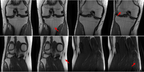
Figure 1: Distribution-shift reconstruction results of a pretrained score network on a knee MRI dataset. The score network was trained on a brain MRI dataset. Images in odd columns are objective reality and those in even columns are sampling results.

Model-driven unrolled networks are built in a different manner: conventional optimization algorithms are unrolled and realized in deep networks, and stacked cascades are used to mimic the iterative steps in the optimization procedure. Compared with data-driven methods, unrolled networks can be better interpreted as those in which conventional priors can be appropriately incorporated, and they have shown convincing results in recent years. Although stacking more cascades can improve the reconstruction performance, large-scale backbone networks can hardly be applied to unrolled networks, considering the limitations of GPU memory, and a trade-off must be established. However, data- and model-driven methods attempt to recover the same target images along different paths, and the complementarity between these methods should be considered. Moreover, we observed the convincing potential of SMLD methods for MRI reconstruction. Current score-matching networks require retraining when applied to different datasets and we observe artifacts on the sampled images without network retraining and subtle tuning of hyperparameters, as shown in Fig. 1. However, we believe that the artifact-affected images can still provide information additional to the known undersampled measurements if the artifacts can be appropriately eliminated, thereby compensating for missing measurements.

Instead of focusing on optimizing the forward and reverse process in SMLD methods, we aim to design a model-driven network which can extract valuable information from naive sampling process and achieve high-quality results robustly. We proposed a novel DL-based hybrid MRI reconstruction workflow, consisting of the following three main steps: (1) Sampling: Using known undersampled raw k-space data, we first obtain samples using SMLD methods. We bypassed all the tuning steps in SMLD methods, such as tuning the hyperparameters or retraining the score networks on our dataset. Instead, we adopted a pretrained score network (PSN) and used the naive samples as preliminary guidance images (PGI) for the follow-up steps. A PSN can be trained using out-of-distribution data. (2) Denoising: We believe that these preliminary reconstructions can provide additional information to guide the reconstruction process through appropriate denoising, leading to a better performance. Considering that the PGIs have relatively low quality and that we observe similar aliasing artifacts in the images, we designed a denoising module (DM) to remove the artifacts from the PGIs. We extracted features from the same score network after fine-tuning and concatenated them with the inputs in Langevin dynamics, which directly produces artifacts, to learn the noise pattern. Then, we used denoised PGIs (DGIs) as higher-quality guidelines for further reconstruction. (3) Guided reconstruction: We designed a densely connected unrolled network to reconstruct the MR images from the undersampled measurements. DGIs are simultaneously input with measurements and periodically updated in the network to guide network training. The DM and unrolled cascades were trained end-to-end.

The experimental results show that although the quality of PGIs is even lower than that of the undersampled measurements, the artifacts were effectively eliminated by the DMs. Meanwhile, the score network can not only help in the sampling process but also cooperate with the unrolled network and improve the denoising performance of the DMs. The proposed reconstruction workflow outperformed state-of-the-art methods through the guidance of DGIs.

The main contributions of this study are summarized as follows:

1. We propose a novel DL-based MRI reconstruction workflow, and low-quality samples obtained using SMLD method are used as guidance during reconstruction.

2. We design an unrolled network, and the initially obtained samples are denoised and periodically updated to guide network training.

3. Experimental results show that without tuning the sampling steps or retraining the score network on target dataset, the low-quality samples can guide the proposed network to obtain robust and high-quality reconstructions, which outperforms the cutting-edge methods.

II Related Works

II-A Conventional approaches for accelerated MRI

For the PI, multiple receiver coils are equipped to obtain raw k-space data simultaneously, and the missing data are recovered by exploiting redundancies among the data from different coils. Sensitivity encoding (SENSE)-type [26] methods work in the image domain, whereas others directly interpolate missing data points in k-space, such as simultaneous acquisition of spatial harmonics (SMASH) [27] and generalized autocalibration partial parallel acquisition (GRAPPA) [28]. However, the reconstructions in PI approaches deteriorate at high acceleration factors. In CS, sparsity-based priors are routinely incorporated to narrow the solution space in the objective functions, and iterative optimization algorithms are designed to approach artifact-free images [29, 30, 31, 32, 33, 34]. However, conventional methods depend heavily on handcrafted procedures, and the iterative steps are time-consuming.

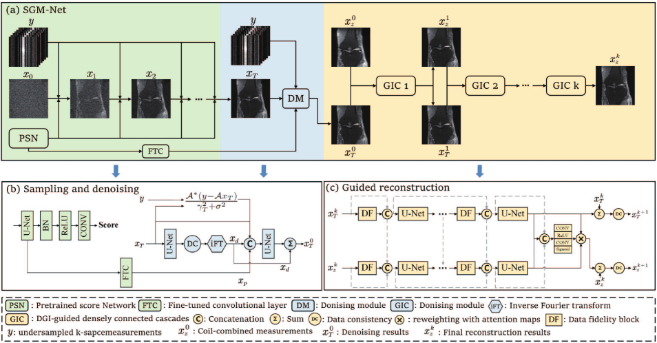
Figure 2: (a) The workflow of the proposed SGM-Net. (b) The network structure of the sampling and denoising steps. (c) The network structure of the $k$th cascade.

II-B Data-driven networks for MRI reconstruction

For data-driven networks trained end-to-end, the mapping between the undersampled measurements and reconstructed images was established. For example, early studies adopted deep convolutional neural networks (CNNs) to reconstruct MR images from zero-filled inputs [35, 36]. The authors in [37] trained the magnitude and phase networks separately in a deep residual network to remove aliasing artifacts. In [38], a complex-valued deep residual network with a higher performance and smaller size was proposed. In addition, GAN-[39, 40]-based networks have shown convincing results [41, 42, 43]. In addition to realizing image domain end-to-end learning, some studies have proposed direct learning mapping in k-space [44] or exploiting the complementarity between the image and k-space domains [9].

Distribution learning is another category of data-driven networks. For example, in [45] the authors used pre-trained generative models to present data distributions. In [23], the authors used score matching to estimate the data distribution, and samples were then generated using annealed Langevin dynamics. Subsequently, the authors proposed improved skills in [24] for higher stability and better performance, and exact log-likelihood computation was supported in [22]. [25] first successfully applied CS-based generative models to overcome the MRI reconstruction problem and showed convincing results in out-of-distribution samples. In [16], the authors further optimized the sampling stage by automatically tuning the hyperparameters using Stein’s unbiased risk estimator (SURE). The authors in [17] proposed a high-frenquency-based diffusion process and accelerated the reverse process. A wavelet-improved technique was proposed in [15] to stably train the score network. In the reverse process, the authors further designed regularization constraints to enhance the robustness. Some works extended the idea of cold diffusion [46] to MRI reconstruction, and the process of adding Gaussian noise is replaced with undersampling operation [47]. However, network retraining is necessary when changing the acquisition parameters, and large datasets are required to fit the mapping [48].

II-C Unrolled networks for MRI reconstruction

Unrolled networks, also known as model-driven networks, are constructed by unrolling iterative optimization steps into deep networks [49, 50, 51, 52, 53]. For example, algorithms such as the alternating direction method of multipliers (ADMM) [49], iterative shrinkage-thresholding algorithm (ISTA) [50], variable splitting (VS) [52], and approximate message passing (AMP) have been successfully applied to solve the objective functions in MRI reconstruction. In [53], the authors extended a previous variational network [51] to learn end-to-end, and sensitivity maps (SM) were estimated in the network. To further improve the accuracy of the SM, different studies [54, 55] have explored ways to simultaneously update the SMs with the reconstructed images. In [56], convolutional blocks were used to extract high-resolution features and transformer blocks have been introduced to refine low-resolution features. The authors of [57] used pre-acquired intra-subject MRI modalities to guide the reconstruction process. In [58], the authors designed a transformer-enhanced network, incorporating a regularization term on the error maps within the residual image domain. Some works solved the optimization problem with structured low-rank algorithm [59, 60, 61]. The authors in [62] designed a deep low-rank and sparse network which explored 1D convolution during training. However, the complementarity between unrolled networks and data-driven methods has not been investigated; in this study, we propose a novel concept in which we treat naive sampling results from SMLD methods as guidance and unrolled cascades as denoising and refining processes.

III Background

In PI, the acquisition of multicoil measurements can be formulated as

$$y=\mathcal{A}x+b$$ (1)

where $y\in\mathbb{C}^{NC}$ is the undersampled k-space data and $C$ is the number of coils. $x\in\mathbb{C}^{M}$ is the underlying MR image for reconstruction and $N<M$. $b$ is the measurement noise. $\mathcal{A}$ is the forward operator given by

$$\mathcal{A}(\cdot)=\mathcal{P}\circ\mathcal{F}\circ\mathcal{E}(\cdot)$$ (2)

where $\mathcal{P}$ denotes the sampling masks that zero the undersampled data points, and $\mathcal{F}$ denotes the Fourier transform matrix. The expanding operator $\mathcal{E}(\cdot)$ calculates the coil-specific images from $x$, defined as

$$\mathcal{E}(x)=(\mathcal{S}_{1}x,\mathcal{S}_{2}x,...),i=1,2,...,C$$ (3)

where $\mathcal{S}_{i}$ is the SM of the $i$th coil. Conversely, the reduced operator $\mathcal{R}$ integrates the coil-specific images into a single image defined as follows:

$$\mathcal{R}(\mathcal{S}_{1}x,\mathcal{S}_{2}x,...)=\sum_{i=1}^{C}\mathcal{S}_{i}x$$ (4)

and the backward operator is expressed as

$$\mathcal{A}^{*}(\cdot)=\mathcal{R}\circ\mathcal{F}^{-1}\circ\mathcal{P}(\cdot)$$ (5)

It is ill-posed to recover missing data directly from $y$. Hence, a regularization term $\lambda\mathcal{U}(x)$ is routinely added to narrow the solution space in the CS, which is

$$\hat{x}=\mathop{\arg\min}\limits_{x}\sum_{i=1}^{C}\|\mathcal{P}\mathcal{F}\mathcal{S}_{i}x-y\|_{2}^{2}+\lambda\mathcal{U}(x)$$ (6)

For example, $\lambda\Psi(x)$ is a common regularization term that imposes the sparsity constraint. Then, gradient descent can be used to solve the problem iteratively as follows:

$$x^{t+1}=x^{t}-\alpha^{t}(\mathcal{A}^{*}(\mathcal{A}x^{t}-y)+\lambda\psi(x^{t}))$$ (7)

where $\alpha^{t}$ is the step size in the $t$th iteration and $\psi(x^{t})$ is the gradient of $\Psi(x)$.

IV Methods

We proposed a score-based generative priors guided model-driven Network (SGM-Net), which is illustrated in Fig. 2. The whole workflow is illustrated in Fig. 2 (a), which comprises three parts: sampling (green components), denoising (blue components), and guided reconstruction (yellow components). The preliminary samples (that is, $x_{T}$ in Fig. 2 (a)) were first obtained using Langevin dynamics and then used as PGIs for the follow-up steps. The gradients of the data distribution were obtained using PSN. Instead of carefully training and tuning the SMLD process to obtain high-quality samples, we sampled $x_{T}$ from an out-of-distribution pretrained network with fitted hyperparameters. Then, we treat the artifacts in $x_{T}$ as removable and propose a DM to eliminate noise and enhance $x_{T}$. The information available from the sampling steps was integrated and fed into the DM, as shown in Fig. 2 (b). Finally, DGIs were used to guide an unrolled network, as shown in Fig. 2 (c). Details of the proposed method are presented in the following subsections.

IV-A Score matching and Langevin dynamics

The first step of the proposed workflow is to obtain PGIs with SMLD to guide the subsequent steps. In this study, we adopted the PSN proposed in [23], which was successfully extended to MRI reconstruction in [25]. To improve the generality of our workflow, the score network was pretrained with out-of-distribution data and tedious tuning and retraining steps were bypassed. The network, remarked as $s_{\theta}$, is a four-cascade RefineNet [63] with dilated convolutions and instance normalization, which is used to approach the score function of $p(x)$ (that is, $\bigtriangledown_{x}\log p(x)$) and we have $s_{\theta}\approx\bigtriangledown_{x}\log p(x)$. Average pooling layers were adopted to replace all maximum pooling layers in RefineNet, and ELU was adopted as the activation function. Then, the annealed Langevin method-based sampling process in MRI can be represented as

$$x_{t+1}=x_{t}+\eta_{t}(s_{\theta}(x_{t};\sigma_{t})+\frac{\mathcal{A}^{*}(y-\mathcal{A}x_{t})}{\gamma_{t}^{2}+\sigma^{2}})+\sqrt{2\eta_{t}}\xi_{t}$$ (8)

where $\xi_{t}\sim\mathcal{N}(0,\textit{I})$ and $t=0,1,2,..,T$. $\eta_{t}$ is the step size in the $t$th iteration and $\eta_{t}=\epsilon\cdot\frac{\sigma^{2}_{j}}{\sigma^{2}_{L}}$. $\{\sigma_{j}\}_{j=1}^{L}$ is a sequence of noise scales that gradually reduces each step size in the annealed Langevin dynamics, where $\sigma_{1}>\sigma_{2}>\cdots>\sigma_{L}$. $\frac{\mathcal{A}^{*}(y-\mathcal{A}x_{t})}{\gamma_{t}^{2}+\sigma^{2}}$ is the consistency term introduced to exploit known measurements. Finally, $x_{T}$ approaches the target as $T$ becomes sufficiently large, which is used as a guide in the follow-up steps.

IV-B Denoising module

Over-smoothing details and hallucination artifacts were observed on the PGIs obtained in the first step, and the denoising step aimed to initially eliminate artifacts and compensate for missing details. First, we designed a KI-branch to learn an denoising mapping from the data between the frequency domain and the image domain. Considering that artifacts usually have different frequencies, which makes it possible to separate them in the k-space, we transferred $x_{T}$ back to the k-space and used a U-Net with a skip connection to learn the mapping to the denoised outputs. Subsequently, U-Net learned to eliminate the noisy signals in k-space. A data consistency (DC) block was concatenated to the U-Net to maintain consistency with the measurements. In addition, the complementarity between the k-space and image domain could also help obtain better performance. We then used an inverse Fourier transform to transfer the k-space data back to the image domain, which is denoted as $x_{d}$, as shown in Fig. 2 (b).

Then, we designed an input-enriched U-Net, marked as $N_{d}$, to further eliminate the noises in $x_{d}$. Fundamentally, the score network is used to generate clean images from noises and the artifacts are generated during the sampling process. Consequently, there could exist an underlying mapping between the artifacts and the elements involved in the sampling process (i.e. equation (8)). Therefore, with the input $x_{T}$ in the DM, we fed $x_{T}$, $s_{\theta}(x_{T};\sigma_{T}$) and $\frac{\mathcal{A}^{*}(y-\mathcal{A}x_{T})}{\gamma_{T}^{2}+\sigma^{2}}$ as the input elements. We fine-tuned $s_{\theta}$, marked as $f_{s_{\theta}}$ that we removed the last batch normalization and activation layers to avoid undesirable loss of information, and concatenated a fine-tuning convolutional (FTC) layer to learn the noise pattern from the features. Only the FTC layer in $f_{s_{\theta}}$ was updated during training. The parameters in the other parts of $f_{s_{\theta}}$ were fitted, and the Langevin sampling results were fed to $f_{s_{\theta}}$ such that the FTC layers could directly learn the noise pattern from the score-matching process for each image.

Besides, to avoid newly introduced noises when obtaining $x_{d}$ from $x_{T}$, $x_{d}$ was also fed to $N_{d}$. Therefore, the enriched input features of $N_{d}$ have four components. By concatenating and feeding the four components into the DM, the denoising process is denoted as:

$$x_{T}^{0}=x_{d}+N_{d}\{x_{p},x_{T},\frac{\mathcal{A}^{*}(y-\mathcal{A}x_{T})}{\gamma_{T}^{2}+\sigma_{T}^{2}},x_{d}\}$$ (9)

where $N_{d}$ is implemented by U-Net, and the common backbone networks are also compatible with learning the mapping. $x_{p}$ is the output of the fine-tuned $f_{s_{\theta}}$. $\{\cdot\}$ implements the channel-wise concatenation of its components. With the skip connection of $x_{d}$, $N_{d}$ can directly learn the mapping to the noise from the enriched inputs. Consequently, the aliasing artifacts are expected to be further eliminated in $x_{T}^{0}$.

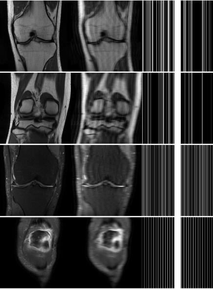
Figure 3: Examples of ground truth images (the first column), undersampled images (the second column) and the corresponding k-space trajectories (the third column). The images from the first and second rows are selected from the Knee dataset with four-fold and six-fold random Cartesian mask. The images from the third and fourth row are selected from the fastMRI dataset with four-fold and six-fold equispaced Cartesian mask.

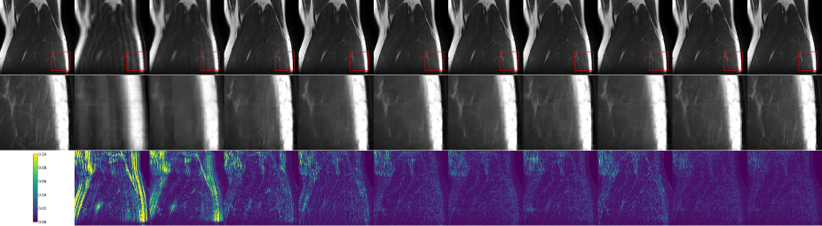
coronal PD 4$\times$ acceleration

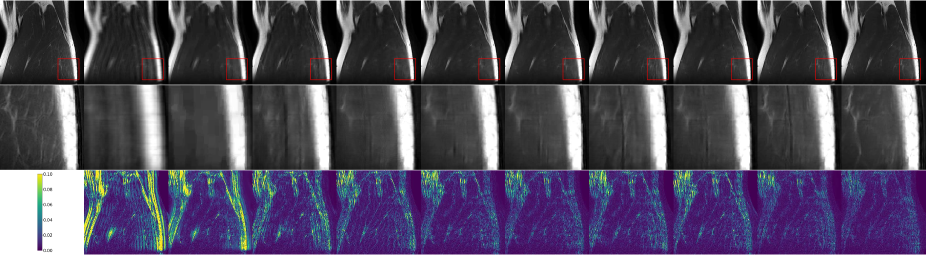
coronal PD 6$\times$ acceleration

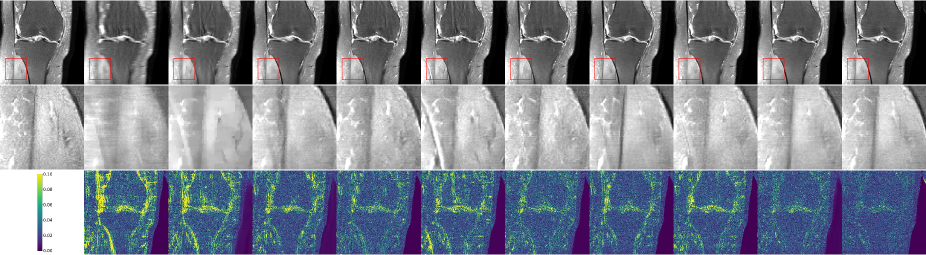
FastMRI 4$\times$ acceleration

FastMRI 6$\times$ acceleration

Figure 4: Examples of the reconstructed images of different methods from coronal PD sequence and FastMRI dataset at 4$\times$ and 6$\times$ acceleration. The first rows of each subfigure are the reconstructed images, the second rows are zoomed details in the red square, and the third rows are the error maps corresponding to the objective reality. The methods from left to right: 1. objective reality; 2. zero-filled; 3. TV; 4. U-Net; 5. D5C5; 6. ISTA-Net; 7. VS-Net; 8. E2EVarNet; 9. ReVarNet; 10. MeDL-Net; 11. SGM-Net (ours).

IV-C Unrolled network with PGI-guided densely-connected cascades

The third step of the proposed workflow is to design an unrolled network to obtain higher-quality reconstructions from denoised guidance images (DGIs) (that is, $x_{T}^{0}$), and the undersampled measurements $x_{z}^{0}$ and $x_{T}^{0}$ are used as two different constraints during unrolled network training. As shown in Fig. 2, the network consists of several DGI-guided densely connected cascades (GICs). The inputs of GICs are $x_{T}^{k}$ and $x_{z}^{k}$ where $k=0,1,...,K$, and $x_{z}^{0}$ is the coil-combined zero-filled image of the undersampled measurements. In each GIC, the undersampled measurements $x_{z}^{k}$ were periodically updated to approach the target images, whereas the DGIs $x_{T}^{k}$ were simultaneously updated to provide more accurate guidance, forming a parallel network structure. $I$ Data fidelity (DF) and $I$ U-Net blocks were alternately stacked in each GIC to solve (7), and U-Net blocks were used to learn the gradient of $\Psi(x)$ from the data. For the $x_{T}^{k}$ branch, the calculations in DF blocks can be represented as

$$r_{T}^{k_{i+1}}=x_{T}^{k_{i}}-\alpha^{k_{i}}(\mathcal{A}^{*}(\mathcal{A}x_{T}^{{k_{i}}}-y)),i=0,1,...,I-1$$ (10)

where $x_{T}^{k_{0}}$ is equal to $x_{T}^{k}$. For the $x_{z}^{k}$-branch, the DF blocks are given by

$$r_{z}^{k_{i+1}}=x_{z}^{k_{i}}-\alpha^{k_{i}}(\mathcal{A}^{*}(\mathcal{A}x_{z}^{k_{i}}-y)),i=0,1,...,I-1$$ (11)

where $x_{z}^{k_{0}}$ is equal to $x_{z}^{k}$. In addition, we propose a densely connected structure to enrich the input information for each U-Net block. For the $x_{T}^{k}$-branch, the initial input and each output of DF blocks corresponding to a U-Net block are concatenated before being fed into U-Net. Therefore, we have:

$$x_{T}^{k_{i+1}}=U_{T}^{i}(\{x_{T}^{k},r_{T}^{k_{1}},r_{T}^{k_{2}},...,r_{T}^{k_{i+1}}\})$$ (12)

where $U_{T}^{i}$ denotes the $i$th U-Net block in the $x_{T}^{k}$-branch, $x_{T}^{k}$ denotes the input to the corresponding branch, and $r_{T}^{k_{i}}$ denotes the output of the $i$th DF block. A similar strategy is implemented in the $x_{z}^{k}$-branch. Considering that we take the final output of the $x_{z}^{k}$ branch in the last GIC as the final reconstruction, the $x_{z}^{k}$ branch is essentially the main branch, and the $x_{T}^{k}$ branch is simultaneously used to guide the reconstruction in the main branch. Therefore, the concatenated information from the $x_{T}^{k}$ branch is also fed to the $x_{z}^{k}$ branch to learn from the features from different stages, represented as

$$x_{z}^{k_{i+1}}=U_{z}^{i}(\{x_{T}^{k},r_{T}^{k_{1}},r_{T}^{k_{2}},...,r_{T}^{k_{i+1}},x_{z}^{k},r_{z}^{k_{1}},r_{z}^{k_{2}},...,r_{z}^{k_{i+1}}\})$$ (13)

After the DF and U-Net blocks, we designed a skip connection and a DC block at the end of the $x_{T}^{k}$ branch, and the produced $x_{T}^{k+1}$ is fed to the next GIC as one of the two inputs as follows:

$$x_{T}^{k+1}=DC(x_{T}^{k}+x_{T}^{k_{I}})$$ (14)

For $x_{z}^{k}$, we further adopted a four-layer attention module (AM) [64] between the last U-Net and skip connection. The information fed to the last DF block is concatenated and simultaneously fed to the AM to produce an attention map

$$M_{A}=AM(\{x_{T}^{k},r_{T}^{k_{1}},r_{T}^{k_{2}},...,r_{T}^{k_{i+1}},x_{z}^{k},r_{z}^{k_{1}},r_{z}^{k_{2}},...,r_{z}^{k_{i+1}}\})$$ (15)

Through a skip connection and DC block, $x_{z}^{k+1}$ is given as

$$x_{z}^{k+1}=DC(x_{z}^{k}+x_{z}^{k_{I}}\odot M_{A}+x_{T}^{k_{I}}\odot((\textbf{J}-M_{A}))$$ (16)

where J is an all-ones matrix and $\odot$ denotes the Hadamard product. Element-wise attention results in a deeper fusion between the two branches and optimizes the intermediate results in each $x_{z}^{k}$ branch.

IV-D loss functions

In this study, the loss function for unrolled network training was designed as

$$Loss=\gamma_{1}(x_{d}+x_{T}^{0}+x_{z}^{K})+\gamma_{2}(\sum_{k=1}^{K}x_{T}^{k}+\sum_{k=1}^{K}x_{z}^{k})$$ (17)

where $x_{d}$ amd $x_{T}^{0}$ are important guidelines for ensuring reconstruction performance, and $x_{z}^{K}$ is the result. $\sum_{k=1}^{K}x_{T}^{k}$ and $\sum_{k=1}^{K}x_{z}^{k}$ are intermediate results. We set $\gamma_{1}=1$ and $\gamma_{2}=0.1$ to distribute more weights for the guidance and results and fewer weights to help the network converge.

IV-E Training details

We adopted the score network $s_{\theta}$ released by the authors in [25], which is pretrained on a brain dataset. We followed the proposed hyperparameters in that manuscript during sampling, and we do not retrain the network on our knee dataset. The numbers of the four-cascade filters were 128, 256, 512, and 1024. The number of filters in the FTC layer is set to 2. In SGM-Net, $K$ is set to five and $I$ is set to three. The numbers of filters in all U-Nets in the DM and GICs were set to 16, 32, 64, and 128. The step size in DF blocks was learned directly in the network. All complex-valued MR images were stored in two channels during the network training. In particular, the first U-Net in DM uses k-space data as input, and the coil channel is combined with the feature channel. Therefore, the number of input and output channels of U-Net was set to 30 (15 coils). The proposed SGM-Net was trained on a UBUNTU 20.04 LTS system with a 3090 GPU (24GB) for 100 epoches, and the learning rate was set to 1e-3. The batch size is set to 1.

V Experiments and Results

V-A Dataset

TABLE I: The quantitative results on Coronal PD and PDFS sequences, as well as the FastMRI dataset, compared with those of cutting-edge methods.

Sequence	Method	PSNR		SSIM
		4×	6×	4×	6×
Coronal PD	zero-filled	31.3089$\pm$3.3939	30.5176$\pm$3.3902	0.8778$\pm$0.0713	0.8626$\pm$0.0799
	TV	33.7498$\pm$3.1753	32.3290$\pm$3.2159	0.8851$\pm$0.0657	0.8658$\pm$0.0725
	U-Net	36.8984$\pm$2.7072	34.7352$\pm$2.7863	0.9361$\pm$0.0610	0.9133$\pm$0.0682
	D5C5	38.7903$\pm$2.8408	35.9697$\pm$2.7990	0.9509$\pm$0.0587	0.9259$\pm$0.0689
	ISTA-Net	39.2910$\pm$2.8423	35.5220$\pm$3.0915	0.9471$\pm$0.0567	0.9138$\pm$0.0717
	VS-Net	40.1649$\pm$2.8767	37.0604$\pm$2.7927	0.9591$\pm$0.0569	0.9358$\pm$0.0648
	E2E-VarNet	39.3592$\pm$2.9368	36.8949$\pm$3.3872	0.9542$\pm$0.0662	0.9342$\pm$0.0775
	ReVarNet	40.1141$\pm$2.8765	37.3681$\pm$2.7867	0.9590$\pm$0.0588	0.9379$\pm$0.0677
	MeDL-Net	40.9295$\pm$2.9072	38.1052$\pm$2.7622	0.9614$\pm$0.0557	0.9417$\pm$0.0663
	SGM-Net (ours)	41.2213$\pm$3.3385	38.4681$\pm$2.9889	0.9638$\pm$0.0642	0.9459$\pm$0.0678
Coronal PDFS	zero-filled	32.0299$\pm$2.0273	31.2221$\pm$2.0575	0.7964$\pm$0.0998	0.7587$\pm$0.1172
	TV	33.7256$\pm$1.9058	32.7328$\pm$1.8850	0.8124$\pm$0.0752	0.7920$\pm$0.0796
	U-Net	34.4367$\pm$0.6572	33.2028$\pm$2.5662	0.8183$\pm$0.0106	0.7758$\pm$0.1222
	D5C5	34.9671$\pm$2.8261	33.4189$\pm$2.4765	0.8250$\pm$0.1106	0.7854$\pm$0.1223
	ISTA-Net	34.4990$\pm$2.6389	33.4569$\pm$2.5758	0.8198$\pm$0.1066	0.7854$\pm$0.1214
	VS-Net	34.6847$\pm$2.7134	33.5010$\pm$2.6100	0.8259$\pm$0.1073	0.7842$\pm$0.1229
	E2E-VarNet	34.6274$\pm$2.7331	33.1626$\pm$2.4742	0.8234$\pm$0.1101	0.7804$\pm$0.1244
	ReVarNet	34.8522$\pm$2.7461	33.3146$\pm$2.5604	0.8272$\pm$0.1080	0.7832$\pm$0.1232
	MeDL-Net	35.5931$\pm$2.7307	34.1409$\pm$2.5501	0.8349$\pm$0.1025	0.7922$\pm$0.1255
	SGM-Net (ours)	35.7932$\pm$3.0718	34.3309$\pm$2.5192	0.8413$\pm$0.1076	0.7978$\pm$0.1242
FastMRI	zero-filled	33.2828$\pm$3.0594	32.5069$\pm$3.0657	0.8857$\pm$0.0709	0.8680$\pm$0.0791
	TV	35.5512$\pm$2.9189	33.8441$\pm$2.8703	0.8884$\pm$0.0635	0.0201$\pm$0.0152
	U-Net	35.21158$\pm$2.5925	33.7864$\pm$2.5331	0.8562$\pm$0.0574	0.8091$\pm$0.0637
	D5C5	36.4550$\pm$3.0246	34.5636$\pm$2.8510	0.9113$\pm$0.0649	0.8849$\pm$0.0749
	ISTA-Net	36.5753$\pm$2.9887	34.6229$\pm$2.8269	0.9134$\pm$0.0656	0.8837$\pm$0.0752
	VS-Net	37.3042$\pm$3.1130	35.5335$\pm$2.8513	0.9202$\pm$0.0637	0.8916$\pm$0.0736
	E2E-VarNet	37.5951$\pm$3.0129	35.6696$\pm$2.8326	0.9217$\pm$0.0635	0.8978$\pm$0.0726
	ReVarNet	37.0047$\pm$3.0130	34.8855$\pm$2.7926	0.9168$\pm$0.0646	0.8895$\pm$0.0746
	MeDL-Net	37.6791$\pm$2.9644	35.9594$\pm$2.7401	0.8984$\pm$0.0643	0.8882$\pm$0.0717
	SGM-Net (ours)	38.9212$\pm$3.4296	37.9430$\pm$3.2521	0.9344$\pm$0.0604	0.9234$\pm$0.0067

In this study, we adopted a publicly available 15-coil knee dataset proposed in [51] to train our model and compared it with other methods. The knee dataset consisted of five 2D turbo spin-echo (TSE) sequences, each of which contained volumes scanned using a 3T scanner from 20 patients. We conducted experiments on coronal proton density (PD; TR=2750 ms, TE=27 ms, in-plane resolution 0.49$\times$0.44 mm², slice thickness 3 mm, 35-42 slices), and coronal fat-saturated PD (PDFS; TR=2870 ms, TE=33 ms, in-plane resolution 0.49$\times$0.44 mm², slice thickness 3 mm, 33-44 slices) sequences. The coil sensitivity maps were precomputed using ESPRIRiT and included in the dataset. The training, validation, and testing sets were randomly divided at a ratio of 3:1:1. Random Cartesian Sampling masks are applied to obtain undersampled measurements with four-fold and six-fold acceleration. 8% lines at the center region are preserved. Examples of training images and the corresponding k-space trajectories are shown in Fig. 3 (the first and second rows).

FastMRI [8] is a publicly available dataset for accelerated MRI, which has been adopted in relevant studies. Considering the limitations of our hardware, we randomly selected a subset of the 15-coil knee dataset to evaluate our model and demonstrate its effectiveness. The data were acquired using the 2D TSE protocol, containing PD and PDFS sequence scanning from 3T or 1.5T systems (TR=2200-3000 ms, TE=27-34 ms, in-plane resolution 0.5$\times$0.5 mm², slice thickness 3 mm). A total of 419, 33, and 375 slices were used for training, validation, and testing sets, respectively. Coil sensitivity maps were not available in the dataset, and related studies have been conducted to estimate and optimize sensitivity maps during training. However, we did not focus on SM estimation in this study and used pretrained SMs in our model to highlight the improvements brought about by the proposed methods. In the fastMRI dataset, we calculated the SMs using the sigpy [65] toolbox. Equispaced Cartesian Sampling masks are applied to obtain undersampled measurements with four-fold and six-fold acceleration. 8% lines at the center region are preserved. Examples of training images and the corresponding k-space trajectories are shown in Fig. 3 (the third and fourth rows).

V-B comparisons with the cutting-edge methods

We compared the proposed SGM-Net with two traditional and seven DL-based methods, as presented in Table I. In the zero-fill method, the missing data in the measurements were filled with zero. The TV method uses total variation as the image prior in a CS-based approach. For DL-based methods (i.e., U-Net [8], D5C5 [66]. ISTA-Net [50] VSNet [52]. E2EVarNet [53], ReVarNet [67]⁶ and MeDL-Net [68]), we adopted the released codes and retrained the networks on our device. We made a concerted effort to keep the announced settings same as those in the corresponding articles, except that we reduced the number of filters in ReVarNet so that all networks could be trained on one GPU. All methods were implemented on the knee dataset (coronal PD and PDFS sequences) and a subset of fastMRI dataset. The PSNR and SSIM results were calculated under four- and six-fold acceleration to evaluate the different methods. As shown in Table I, the proposed SGM-Net robustly achieves the best results on all the datasets with different acceleration factors. The reconstruction results of the sample images are presented in Fig.4. We can observe from the zoomed region (second rows) that our method recovered the most details, and the error maps (third row) exhibited the least errors.

V-C Ablation Studies

TABLE II: Results of ablation studies on coronal PD sequence with four- and six-fold acceleration rates.

Method	PSNR		SSIM
	4×	6×	4×	6×
SG	26.8198$\pm$4.7495	25.0439$\pm$7.2973	0.4172$\pm$0.1712	0.5212$\pm$0.1568
MN	38.8362$\pm$2.6402	35.9488$\pm$2.6333	0.8623$\pm$0.0880	0.7861$\pm$0.1088
SR-MN	35.4585$\pm$2.9562	33.2093$\pm$2.6398	0.8351$\pm$0.0912	0.7412$\pm$0.1284
SG-MN-DM-US	40.7095$\pm$3.0165	38.0227$\pm$2.9647	0.9619$\pm$0.0615	0.9440$\pm$0.0700
SG-MN-DM-DG	40.8443$\pm$3.0384	38.2183$\pm$2.9986	0.9629$\pm$0.0624	0.9448$\pm$0.0721
SG-MN-US-DG	41.0424$\pm$3.4144	38.1616$\pm$2.9985	0.9633$\pm$0.0676	0.9443$\pm$0.0714
SG-MN-DM-US-DG	41.2213$\pm$3.3385	38.4681$\pm$2.9889	0.9638$\pm$0.0642	0.9459$\pm$0.0678

To highlight the improvements brought by different modules, we designed several workflows for a clear evaluation. Specifically, the proposed modules for evaluation were the SMLD-based guidance (SG), model-driven network structure (MN), denoising module (DM), updating steps (US) for SGs, and densely connected guidance (DG) in the unrolled network. The ablations was designed as follows.

1. SG: using the SMLD results as the final reconstructions.

2. MN: a standard unrolled network with the undersampled measurements as the inputs.

3. SG-MN: a standard unrolled network with SMLD results as the inputs.

4. SG-MN-DM-US: the densely connected structure is removed from all the cascades.

5. SG-MN-DM-DG: the SMLD results are used as guidance in the unrolled network but without and updating steps.

6. SG-MN-US-DG: the SMLD results are used to guide the network without denoising in the DM.

7. SG-MN-DM-US-DG: the proposed SGM-Net.

The quantitative results are shown in table II. Comparing SG with the proposed SGM-Net, we can observe a significant improvement brought about by the proposed modules, whereas the average results from the SMLD sampling are worse than those of the zero-filled method. Similarly, through the guidance of the SMLD results, the results of the unrolled MN method were significantly improved with guidance from the SMLD results. Using either of these two methods alone can’t achieve satisfactory results. Moreover, we simply combine SR and MN in the SR-MN workflow that the SMLD results are directly fed to the network as input. However, the performance are even worse than that of MN. This phenomenon demonstrates the effectiveness of the proposed guidance-based workflow, which outperforms a simple combination of the two methods.

A comparison between SG-MN-DM-US and SGM-Net demonstrated that the densely connected structure is capable of fulfilling the guiding work and improving the final results. Removing the densely connected structure and using only the AMs to optimize the reconstructed images will lead to a degredation in the final results. By comparing SG-MN-DM-DG with SGM-Net, we observed that the updating steps in the proposed model can ensured that accurate guidance was provided by the PGIs and improved the results. When removing the DM and directly feeding SMLD results to guide the network, the reconstruction performances of SG-MN-US-DG are similarly worse than that of SGM-Net. The best results are achieved with the integration of all the proposed modules, which demonstrates their effectiveness and necessity. Furthermore, we illustrate in subsection V.E that the integration of the proposed module can enhance the robustness of the network with greatly reduced training data.

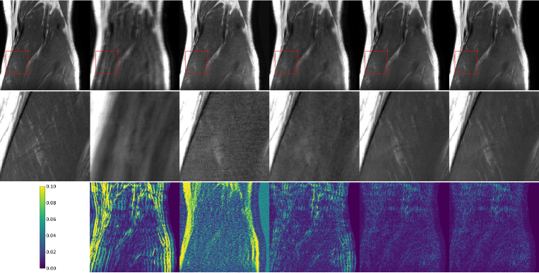
Figure 5: The reconstruction results of the original model at four-fold acceleration. The first rows of each subfigure are the reconstructed images, the second rows are zoomed details in the red square, and the third rows are the error maps representing the objective reality. The corresponding images from left to right: the objective reality, zero-filled measurements, PGI, DGI, and the final output of $x_{z}^{k}$ and $x_{T}^{k}$ branch.

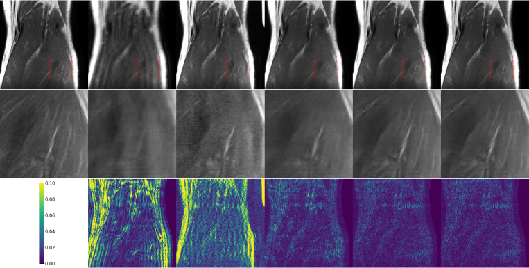
Figure 6: The reconstruction results with 20% sampling steps at four-fold acceleration. The first rows of each subfigure are the reconstructed images, the second rows are zoomed details in the red square, and the third rows are the error maps representing the objective reality. The corresponding images from left to right: the objective reality, zero-filled measurements, PGI, DGI, and the final output of $x_{z}^{k}$ and $x_{T}^{k}$ branch.

TABLE III: Quantitative results of the selected images at four-fold and six-fold acceleration rates.

Method	Image	PSNR		SSIM
		4×	6×	4×	6×
	zero-filled	31.3089$\pm$3.3939	30.5176$\pm$3.3902	0.8778$\pm$0.0713	0.8626$\pm$0.0799
original	$x_{T}$	26.8198$\pm$4.7495	25.0439$\pm$7.2973	0.4172$\pm$0.1712	0.5212$\pm$0.1568
	$x_{T}^{0}$	39.0871$\pm$2.5214	37.0431$\pm$2.3824	0.9523$\pm$0.0587	0.9364$\pm$0.0635
	$x_{T}^{K}$	41.0913$\pm$3.4621	38.3504$\pm$2.9553	0.9635$\pm$0.0656	0.9458$\pm$0.0678
	$x_{z}^{K}$	41.2213$\pm$3.3385	38.4681$\pm$2.9889	0.9638$\pm$0.0642	0.9459$\pm$0.0678
20% sampling steps	$x_{T}$	19.7481$\pm$7.8121	17.5994$\pm$7.7102	0.4664$\pm$0.2049	0.4312$\pm$0.1723
	$x_{T}^{0}$	38.4951$\pm$2.9590	36.4403$\pm$2.9405	0.9500$\pm$0.0600	0.9317$\pm$0.0656
	$x_{T}^{K}$	40.8341$\pm$3.8591	38.2336$\pm$3.0403	0.9631$\pm$0.0654	0.9421$\pm$0.0691
	$x_{z}^{K}$	40.9907$\pm$3.7419	38.3414$\pm$2.8912	0.9631$\pm$0.0657	0.9446$\pm$0.0682
pretrained with another dataset	$x_{T}$	25.5783$\pm$4.7741	24.2301$\pm$7.8034	0.4904$\pm$0.1506	0.4692$\pm$0.1549
	$x_{T}^{0}$	39.0112$\pm$2.7413	36.8603$\pm$2.7916	0.9510$\pm$0.0578	0.9351$\pm$0.6225
	$x_{T}^{K}$	40.9581$\pm$3.3235	38.2714$\pm$2.8405	0.9634$\pm$0.0663	0.9401$\pm$0.0702
	$x_{z}^{K}$	41.0920$\pm$3.2329	38.4204$\pm$2.9084	0.9636$\pm$0.6828	0.9432$\pm$0.0688

V-D Evaluation of the guided reconstruction process

To evaluate the improvements brought by the guided process, we plotted the following images: the image of the ground truth, zero-filled measurements, PGI ($x_{T}$), DGI ($x_{T}^{0}$), and the final output of $x_{z}^{k}$ and $x_{T}^{k}$ branches ($x_{T}^{K}$ and $x_{z}^{K}$) of an MR image from the test dataset. To mitigate potential influences from the sampling process, we designed the following three sampling methods:

1. original: the SMLD results are sampled using the pretrained score network, as described previously.

2. 20% sampling steps: the SMLD results are sampled using the pretrained score network, but using only 20% of the original sampling steps.

3. pretrained with another dataset: we continued to train the score network on another brain dataset proposed in [69], and the images are sampled with the same hyperparameters in the original method.

The reconstructed images from the original sampling method at four-fold acceleration are shown in Fig. 5. The first row shows the corresponding images, and the second row shows the magnified details. The zero-filled image (second column) is blurred, and the PGI (third column) loses texture details. However, the artifacts in the DGI (fourth column) were effectively eliminated from the zero-filled image and PGI by DMs. Then, the GICs recovered the missing details in the DGIs and $x_{T}^{K}$ (fifth column) and $x_{z}^{K}$ (sixth column) presented satisfactory results when compared with the ground truth images (first column). The error maps in the third row exhibit that the massive errors in the zero-filled images and PGIs are obviously alleviated, the the image quality are further improved in $x_{T}^{K}$ and $x_{z}^{K}$. The reconstructed images with 20% sampling steps at four-fold acceleration are depicted in Fig. 6, which are also consistent with the observations in Fig. 5.

The quantitative results for the three sampling methods are presented in Table III. $x_{z}^{K}$, which is chosen as the final result, slightly outperforms $x_{T}^{K}$, and the other results obtained at four- or six-fold acceleration are consistent with the results observed from the images. Significantly reducing the sampling steps leads to further deterioration in the quality of SMLD results. However, the impact on the final reconstruction results is minimal, demonstrating the robustness of our proposed method to noise input, and the DMs are effective to extract valuable information from the noise input. We continue training the score network on another brain dataset to make perturbations on the pretrained model, which produces reconstructions of equally high quality through our workflow, demonstrating that our method imposes minimal requirements on the sampling process. In summary, this experiment vividly illustrates how our proposed workflow leverages SMLD results to extract crucial information, aiding in the reconstruction process and finally achieving high-quality results.

V-E Evaluation of the network robustness

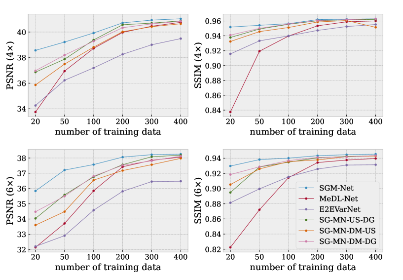
Figure 7: PSNR (the first column) and SSIM (the second column) results of SGM-Net, MeDL-Net, and E2EVarNet with different amounts of training data at four- (the first row) and six-fold (the second row).

In this subsection we illustrate the network robustness with limited training data. Here, we compared E2E-VarNet and MeDL-Net, which have convincing performances and do not leverage guidance images, as shown in Table I. We also compared with three ablation networks (i.e. SG-MN-DM-US, SG-MN-MN-DG and SG-MN-US-DG). We reduced the number of training images of the different methods to different extents and compared their performances with our model. The results are presented in Fig. 7. We compared the PSNR and SSIM results of the above networks at four- and six-fold, respectively. We observed that the performances of the other networks deteriorated with decreasing training data. Meanwhile, the performance of SGM-Net was more stable even with only 20 training images. Compared with E2E-VarNet and MeDL-Net, our ablation networks also exhibit relatively better robustness. However, the degradation of image quality become more pronounced with the decrease of training data, which further demonstrating the necessity of the proposed modules. To sum up, this experiment demonstrates that proposed guidance process can effectively compensate for information in the missing training data and make the model robust.

VI Discussions

To make the sampling process robust and achieve better performance, most of the cutting-edge methods proposed to optimize the training of the generative models or the sampling steps. For example, the authors in [14] fed high-dimensional tensors to a noise conditional score network during training, and they designed homotopic iterations at the inference phase. The authors in [13] proposed a framework named score-POCS. During inference, the reconstruction process iterates between SDE solvers and data consistency steps. Compared with them, the most significant distinction in our workflow is that we bypass all the tedious hyperparameter tuning and network retraining steps and implement a naive sampling. The reconstruction performances are then not robust especially with distribution-shift test datasets, and the results are observed to be severely corrupted. We novelly treat the SMLD results as a generalized prior, and we design an unrolled network which can extract valuable information from the SMLD samples to guide reconstruction, while the components during sampling can also help to eliminate the artifacts in the network. Experimental results have demonstrated that compared with the naive sampling results, only small amounts of data are required to train the unrolled network and the performances can be greatly improved.

Another bottleneck in diffusion models is that the sampling process is relatively slow. To solve this problem, the authors in [70] proposed DiffuseRecon, and the reverse process can be guided with observed k-space signal. The authors designed a coarse-to-fine algorithm to save sampling time. In [71], the authors proposed deep ensemble denoisers and incorporated them with score-based generative models to reconstructed images. Consequently, the necessary iterations are reduced. In our workflow, we preserved the naive sampling process. However, the unrolled network have good tolerance to artifact-affected inputs, hence the sampling steps can also be great reduced.

In the proposed reconstruction workflow, the low-quality SMLD samples have been demonstrated to be effective to guide the network training and improve the final results. Meanwhile, the proposed workflow is also compatible to optimized SMLD steps with higher quality references, which show great potential to be exploited in future works. Besides, a limitation of the proposed method is that although the workflow exhibits considerable tolerance for the SMLD process, the unrolled network still requires some data for training to achieve superior performance. Training strategies such as self-supervising should be considered to further optimize the workflow in future works.

VII Conclusions

In this study, we proposed a novel workflow to eliminate the need for optimizing the forward and reverse process in the SMLD-based method for MRI reconstruction. Instead, an unrolled model-driven network is proposed to extract valuable information from naive sampling results. Subsequently, the SMLD results can be periodically updated and utilized to guide the network training process. The experimental results demonstrated that the proposed hybrid method outperforms the workflows solely based on diffusion models or unrolled networks. Additionally, our method alleviates the substantial requirements for sampling steps and training images. When compared with cutting-edge methods, our network consistently produces reconstructions of higher quality, showcasing its superiority in MRI reconstruction tasks.

References

- [1] D. J. Larkman and R. G. Nunes, “Parallel magnetic resonance imaging,” Physics in Medicine & Biology, vol. 52, no. 7, p. R15, 2007.
- [2] K. P. Pruessmann, “Encoding and reconstruction in parallel mri,” NMR in Biomedicine: An International Journal Devoted to the Development and Application of Magnetic Resonance In vivo, vol. 19, no. 3, pp. 288–299, 2006.
- [3] M. Lustig, D. Donoho, and J. M. Pauly, “Sparse mri: The application of compressed sensing for rapid mr imaging,” Magnetic Resonance in Medicine: An Official Journal of the International Society for Magnetic Resonance in Medicine, vol. 58, no. 6, pp. 1182–1195, 2007.
- [4] M. Lustig, D. L. Donoho, J. M. Santos, and J. M. Pauly, “Compressed sensing mri,” IEEE signal processing magazine, vol. 25, no. 2, pp. 72–82, 2008.
- [5] J. C. Ye, “Compressed sensing mri: a review from signal processing perspective,” BMC Biomedical Engineering, vol. 1, no. 1, pp. 1–17, 2019.
- [6] C. M. Sandino, J. Y. Cheng, F. Chen, M. Mardani, J. M. Pauly, and S. S. Vasanawala, “Compressed sensing: From research to clinical practice with deep neural networks: Shortening scan times for magnetic resonance imaging,” IEEE signal processing magazine, vol. 37, no. 1, pp. 117–127, 2020.
- [7] D. Liang, J. Cheng, Z. Ke, and L. Ying, “Deep magnetic resonance image reconstruction: Inverse problems meet neural networks,” IEEE Signal Processing Magazine, vol. 37, no. 1, pp. 141–151, 2020.
- [8] J. Zbontar, F. Knoll, A. Sriram, T. Murrell, Z. Huang, M. J. Muckley, A. Defazio, R. Stern, P. Johnson, M. Bruno et al., “fastmri: An open dataset and benchmarks for accelerated mri,” arXiv preprint arXiv:1811.08839, 2018.
- [9] T. Eo, Y. Jun, T. Kim, J. Jang, H.-J. Lee, and D. Hwang, “Kiki-net: cross-domain convolutional neural networks for reconstructing undersampled magnetic resonance images,” Magnetic resonance in medicine, vol. 80, no. 5, pp. 2188–2201, 2018.
- [10] D. Hu, Y. Zhang, W. Li, W. Zhang, K. Reddy, Q. Ding, X. Zhang, Y. Chen, and H. Gao, “Sea-net: Structure-enhanced attention network for limited-angle cbct reconstruction of clinical projection data,” IEEE Transactions on Instrumentation and Measurement, 2023.
- [11] A. Kazerouni, E. K. Aghdam, M. Heidari, R. Azad, M. Fayyaz, I. Hacihaliloglu, and D. Merhof, “Diffusion models in medical imaging: A comprehensive survey,” Medical Image Analysis, p. 102846, 2023.
- [12] Y. Korkmaz, T. Cukur, and V. M. Patel, “Self-supervised mri reconstruction with unrolled diffusion models,” in International Conference on Medical Image Computing and Computer-Assisted Intervention. Springer, 2023, pp. 491–501.
- [13] H. Chung and J. C. Ye, “Score-based diffusion models for accelerated mri,” Medical image analysis, vol. 80, p. 102479, 2022.
- [14] C. Quan, J. Zhou, Y. Zhu, Y. Chen, S. Wang, D. Liang, and Q. Liu, “Homotopic gradients of generative density priors for mr image reconstruction,” IEEE Transactions on Medical Imaging, vol. 40, no. 12, pp. 3265–3278, 2021.
- [15] W. Wu, Y. Wang, Q. Liu, G. Wang, and J. Zhang, “Wavelet-improved score-based generative model for medical imaging,” IEEE transactions on medical imaging, 2023.
- [16] B. Ozturkler, C. Liu, B. Eckart, M. Mardani, J. Song, and J. Kautz, “Smrd: Sure-based robust mri reconstruction with diffusion models,” in International Conference on Medical Image Computing and Computer-Assisted Intervention. Springer, 2023, pp. 199–209.
- [17] C. Cao, Z.-X. Cui, Y. Wang, S. Liu, T. Chen, H. Zheng, D. Liang, and Y. Zhu, “High-frequency space diffusion model for accelerated mri,” IEEE Transactions on Medical Imaging, 2024.
- [18] J. Ho, A. Jain, and P. Abbeel, “Denoising diffusion probabilistic models,” Advances in neural information processing systems, vol. 33, pp. 6840–6851, 2020.
- [19] Z. Wang, R. Feng, J. Mao, X. Tao, D. Zhang, X. Shan, and J. Zhou, “Srfs: Super resolution in fast-slow scanning mode of sem based on denoising diffusion probability model,” IEEE Transactions on Instrumentation and Measurement, 2024.
- [20] Q. Liu, J. Lee, and M. Jordan, “A kernelized stein discrepancy for goodness-of-fit tests,” in International conference on machine learning. PMLR, 2016, pp. 276–284.
- [21] A. Hyvärinen and P. Dayan, “Estimation of non-normalized statistical models by score matching.” Journal of Machine Learning Research, vol. 6, no. 4, 2005.
- [22] Y. Song, J. Sohl-Dickstein, D. P. Kingma, A. Kumar, S. Ermon, and B. Poole, “Score-based generative modeling through stochastic differential equations,” arXiv preprint arXiv:2011.13456, 2020.
- [23] Y. Song and S. Ermon, “Generative modeling by estimating gradients of the data distribution,” Advances in neural information processing systems, vol. 32, 2019.
- [24] ——, “Improved techniques for training score-based generative models,” Advances in neural information processing systems, vol. 33, pp. 12 438–12 448, 2020.
- [25] A. Jalal, M. Arvinte, G. Daras, E. Price, A. G. Dimakis, and J. Tamir, “Robust compressed sensing mri with deep generative priors,” Advances in Neural Information Processing Systems, vol. 34, pp. 14 938–14 954, 2021.
- [26] K. P. Pruessmann, M. Weiger, M. B. Scheidegger, and P. Boesiger, “Sense: sensitivity encoding for fast mri,” Magnetic Resonance in Medicine: An Official Journal of the International Society for Magnetic Resonance in Medicine, vol. 42, no. 5, pp. 952–962, 1999.
- [27] D. K. Sodickson and W. J. Manning, “Simultaneous acquisition of spatial harmonics (smash): fast imaging with radiofrequency coil arrays,” Magnetic resonance in medicine, vol. 38, no. 4, pp. 591–603, 1997.
- [28] M. A. Griswold, P. M. Jakob, R. M. Heidemann, M. Nittka, V. Jellus, J. Wang, B. Kiefer, and A. Haase, “Generalized autocalibrating partially parallel acquisitions (grappa),” Magnetic Resonance in Medicine: An Official Journal of the International Society for Magnetic Resonance in Medicine, vol. 47, no. 6, pp. 1202–1210, 2002.
- [29] K. T. Block, M. Uecker, and J. Frahm, “Undersampled radial mri with multiple coils. iterative image reconstruction using a total variation constraint,” Magnetic Resonance in Medicine: An Official Journal of the International Society for Magnetic Resonance in Medicine, vol. 57, no. 6, pp. 1086–1098, 2007.
- [30] L. Feng, M. B. Srichai, R. P. Lim, A. Harrison, W. King, G. Adluru, E. V. Dibella, D. K. Sodickson, R. Otazo, and D. Kim, “Highly accelerated real-time cardiac cine mri using k–t sparse-sense,” Magnetic resonance in medicine, vol. 70, no. 1, pp. 64–74, 2013.
- [31] F. Knoll, K. Bredies, T. Pock, and R. Stollberger, “Second order total generalized variation (tgv) for mri,” Magnetic resonance in medicine, vol. 65, no. 2, pp. 480–491, 2011.
- [32] J. Fessler, “Optimization methods for magnetic resonance image reconstruction: Key models and optimization algorithms,” IEEE Signal Proc Mag, vol. 37, no. 1, pp. 33–40, 2020.
- [33] S. Ramani and J. Fessler, “Parallel mr image reconstruction using augmented lagrangian methods,” IEEE transactions on medical imaging, vol. 30, no. 3, pp. 694–706, 2010.
- [34] J. Huang, S. Zhang, and D. Metaxas, “Efficient mr image reconstruction for compressed mr imaging,” Medical Image Analysis, vol. 15, no. 5, pp. 670–679, 2011.
- [35] S. Wang, Z. Su, L. Ying, X. Peng, S. Zhu, F. Liang, D. Feng, and D. Liang, “Accelerating magnetic resonance imaging via deep learning,” in 2016 IEEE 13th international symposium on biomedical imaging (ISBI). IEEE, 2016, pp. 514–517.
- [36] J. C. Ye, Y. Han, and E. Cha, “Deep convolutional framelets: A general deep learning framework for inverse problems,” SIAM Journal on Imaging Sciences, vol. 11, no. 2, pp. 991–1048, 2018.
- [37] D. Lee, J. Yoo, S. Tak, and J. C. Ye, “Deep residual learning for accelerated mri using magnitude and phase networks,” IEEE Transactions on Biomedical Engineering, vol. 65, no. 9, pp. 1985–1995, 2018.
- [38] S. Wang, H. Cheng, L. Ying, T. Xiao, Z. Ke, H. Zheng, and D. Liang, “Deepcomplexmri: Exploiting deep residual network for fast parallel mr imaging with complex convolution,” Magnetic Resonance Imaging, vol. 68, pp. 136–147, 2020.
- [39] I. Goodfellow, J. Pouget-Abadie, M. Mirza, B. Xu, D. Warde-Farley, S. Ozair, A. Courville, and Y. Bengio, “Generative adversarial nets,” Advances in neural information processing systems, vol. 27, 2014.
- [40] J. Gui, Z. Sun, Y. Wen, D. Tao, and J. Ye, “A review on generative adversarial networks: Algorithms, theory, and applications,” IEEE transactions on knowledge and data engineering, vol. 35, no. 4, pp. 3313–3332, 2021.
- [41] G. Yang, S. Yu, H. Dong, G. Slabaugh, P. L. Dragotti, X. Ye, F. Liu, S. Arridge, J. Keegan, Y. Guo et al., “Dagan: Deep de-aliasing generative adversarial networks for fast compressed sensing mri reconstruction,” IEEE transactions on medical imaging, vol. 37, no. 6, pp. 1310–1321, 2017.
- [42] M. Mardani, E. Gong, J. Y. Cheng, S. S. Vasanawala, G. Zaharchuk, L. Xing, and J. M. Pauly, “Deep generative adversarial neural networks for compressive sensing mri,” IEEE transactions on medical imaging, vol. 38, no. 1, pp. 167–179, 2018.
- [43] T. M. Quan, T. Nguyen-Duc, and W.-K. Jeong, “Compressed sensing mri reconstruction using a generative adversarial network with a cyclic loss,” IEEE transactions on medical imaging, vol. 37, no. 6, pp. 1488–1497, 2018.
- [44] Y. Han, L. Sunwoo, and J. C. Ye, “k-space deep learning for accelerated mri,” IEEE transactions on medical imaging, vol. 39, no. 2, pp. 377–386, 2019.
- [45] A. Bora, A. Jalal, E. Price, and A. G. Dimakis, “Compressed sensing using generative models,” in International conference on machine learning. PMLR, 2017, pp. 537–546.
- [46] A. Bansal, E. Borgnia, H.-M. Chu, J. Li, H. Kazemi, F. Huang, M. Goldblum, J. Geiping, and T. Goldstein, “Cold diffusion: Inverting arbitrary image transforms without noise,” Advances in Neural Information Processing Systems, vol. 36, 2024.
- [47] J. Huang, A. I. Aviles-Rivero, C.-B. Schönlieb, and G. Yang, “Cdiffmr: Can we replace the gaussian noise with k-space undersampling for fast mri?” in International Conference on Medical Image Computing and Computer-Assisted Intervention. Springer, 2023, pp. 3–12.
- [48] S. Wang, T. Xiao, Q. Liu, and H. Zheng, “Deep learning for fast mr imaging: A review for learning reconstruction from incomplete k-space data,” Biomedical Signal Processing and Control, vol. 68, p. 102579, 2021.
- [49] J. Sun, H. Li, Z. Xu et al., “Deep admm-net for compressive sensing mri,” Advances in neural information processing systems, vol. 29, 2016.
- [50] J. Zhang and B. Ghanem, “Ista-net: Interpretable optimization-inspired deep network for image compressive sensing,” in Proceedings of the IEEE conference on computer vision and pattern recognition, 2018, pp. 1828–1837.
- [51] K. Hammernik, T. Klatzer, E. Kobler, M. P. Recht, D. K. Sodickson, T. Pock, and F. Knoll, “Learning a variational network for reconstruction of accelerated mri data,” Magnetic resonance in medicine, vol. 79, no. 6, pp. 3055–3071, 2018.
- [52] J. Duan, J. Schlemper, C. Qin, C. Ouyang, W. Bai, C. Biffi, G. Bello, B. Statton, D. P. O’regan, and D. Rueckert, “Vs-net: Variable splitting network for accelerated parallel mri reconstruction,” in Medical Image Computing and Computer Assisted Intervention–MICCAI 2019: 22nd International Conference, Shenzhen, China, October 13–17, 2019, Proceedings, Part IV 22. Springer, 2019, pp. 713–722.
- [53] A. Sriram, J. Zbontar, T. Murrell, A. Defazio, C. L. Zitnick, N. Yakubova, F. Knoll, and P. Johnson, “End-to-end variational networks for accelerated mri reconstruction,” in Medical Image Computing and Computer Assisted Intervention–MICCAI 2020: 23rd International Conference, Lima, Peru, October 4–8, 2020, Proceedings, Part II 23. Springer, 2020, pp. 64–73.
- [54] Y. Jun, H. Shin, T. Eo, and D. Hwang, “Joint deep model-based mr image and coil sensitivity reconstruction network (joint-icnet) for fast mri,” in Proceedings of the IEEE/CVF Conference on Computer Vision and Pattern Recognition, 2021, pp. 5270–5279.
- [55] M. Arvinte, S. Vishwanath, A. H. Tewfik, and J. I. Tamir, “Deep j-sense: Accelerated mri reconstruction via unrolled alternating optimization,” in International conference on medical image computing and computer-assisted intervention. Springer, 2021, pp. 350–360.
- [56] Z. Fabian, B. Tinaz, and M. Soltanolkotabi, “Humus-net: Hybrid unrolled multi-scale network architecture for accelerated mri reconstruction,” Advances in Neural Information Processing Systems, vol. 35, pp. 25 306–25 319, 2022.
- [57] K. Sun, Q. Wang, and D. Shen, “Joint cross-attention network with deep modality prior for fast mri reconstruction,” IEEE Transactions on Medical Imaging, 2023.
- [58] D. Hu, Y. Zhang, J. Zhu, Q. Liu, and Y. Chen, “Trans-net: Transformer-enhanced residual-error alternative suppression network for mri reconstruction,” IEEE Transactions on Instrumentation and Measurement, vol. 71, pp. 1–13, 2022.
- [59] A. Pramanik, H. K. Aggarwal, and M. Jacob, “Deep generalization of structured low-rank algorithms (deep-slr),” IEEE transactions on medical imaging, vol. 39, no. 12, pp. 4186–4197, 2020.
- [60] X. Zhang, H. Lu, D. Guo, Z. Lai, H. Ye, X. Peng, B. Zhao, and X. Qu, “Accelerated mri reconstruction with separable and enhanced low-rank hankel regularization,” IEEE Transactions on Medical Imaging, vol. 41, no. 9, pp. 2486–2498, 2022.
- [61] T. Qiu, W. Liao, Y. Huang, J. Wu, D. Guo, D. Liu, X. Wang, J.-F. Cai, B. Hu, and X. Qu, “An automatic denoising method for nmr spectroscopy based on low-rank hankel model,” IEEE Transactions on Instrumentation and Measurement, vol. 70, pp. 1–12, 2021.
- [62] Z. Wang, C. Qian, D. Guo, H. Sun, R. Li, B. Zhao, and X. Qu, “One-dimensional deep low-rank and sparse network for accelerated mri,” IEEE Transactions on Medical Imaging, vol. 42, no. 1, pp. 79–90, 2022.
- [63] G. Lin, A. Milan, C. Shen, and I. Reid, “Refinenet: Multi-path refinement networks for high-resolution semantic segmentation,” in Proceedings of the IEEE conference on computer vision and pattern recognition, 2017, pp. 1925–1934.
- [64] X. Qiao, W. Li, G. Wang, and Y. Huang, “A collaborative model-driven network for mri reconstruction,” arXiv preprint arXiv:2402.03383, 2024.
- [65] J. Martin, F. Ong, J. Ma, J. Tamir, M. Lustig, and W. Grissom, “Sigpy. rf: comprehensive open-source rf pulse design tools for reproducible research,” in Proc. 28th Annual Meeting of ISMRM, 2020.
- [66] J. Schlemper, J. Caballero, J. Hajnal, A. Price, and D. Rueckert, “A deep cascade of convolutional neural networks for dynamic mr image reconstruction,” IEEE transactions on medical imaging, vol. 37, no. 2, pp. 491–503, 2017.
- [67] G. Yiasemis, C. Sánchez, J. Sonke, and J. Teuwen, “Recurrent variational network: A deep learning inverse problem solver applied to the task of accelerated mri reconstruction,” arXiv preprint arXiv:2111.09639, 2021.
- [68] X. Qiao, Y. Huang, and W. Li, “Medl-net: A model-based neural network for mri reconstruction with enhanced deep learned regularizers,” Magnetic Resonance in Medicine, vol. 89, no. 5, pp. 2062–2075, 2023.
- [69] H. K. Aggarwal, M. P. Mani, and M. Jacob, “Modl: Model-based deep learning architecture for inverse problems,” IEEE transactions on medical imaging, vol. 38, no. 2, pp. 394–405, 2018.
- [70] C. Peng, P. Guo, S. K. Zhou, V. M. Patel, and R. Chellappa, “Towards performant and reliable undersampled mr reconstruction via diffusion model sampling,” in International Conference on Medical Image Computing and Computer-Assisted Intervention. Springer, 2022, pp. 623–633.
- [71] R. Hou, F. Li, and T. Zeng, “Fast and reliable score-based generative model for parallel mri,” IEEE Transactions on Neural Networks and Learning Systems, 2023.