Accelerating Legacy Numerical Solvers by Non-intrusive Gradient-based Meta-solving

Abstract

Scientific computing is an essential tool for scientific discovery and engineering design, and its computational cost is always a main concern in practice. To accelerate scientific computing, it is a promising approach to use machine learning (especially meta-learning) techniques for selecting hyperparameters of traditional numerical methods. There have been numerous proposals to this direction, but many of them require automatic-differentiable numerical methods. However, in reality, many practical applications still depend on well-established but non-automatic-differentiable legacy codes, which prevents practitioners from applying the state-of-the-art research to their own problems. To resolve this problem, we propose a non-intrusive methodology with a novel gradient estimation technique to combine machine learning and legacy numerical codes without any modification. We theoretically and numerically show the advantage of the proposed method over other baselines and present applications of accelerating established non-automatic-differentiable numerical solvers implemented in PETSc, a widely used open-source numerical software library.

1 Introduction

Scientific Machine Learning (SciML) is an emerging research area, where scientific data and advancing Machine Learning (ML) techniques are utilized for new data-driven scientific discovery (Baker et al., 2019; Takamoto et al., 2022; Cuomo et al., 2022). One of the important topics in SciML is ML-enhanced simulation that leverages the strengths of both ML and traditional scientific computing, and recently numerous methods have been proposed to this direction (Karniadakis et al., 2021; Thuerey et al., 2021; Vinuesa & Brunton, 2021; Willard et al., 2022). These hybrid methods can be categorized into two groups according to how they are trained: separately or jointly.

In the first group, ML models are trained separately from numerical solvers and combined after training. Typically, they are trained to predict the solution of the target problem, and the solver uses the prediction as an initial guess (Ajuria Illarramendi et al., 2020; Özbay et al., 2021; Huang et al., 2020; Vaupel et al., 2020; Venkataraman & Amos, 2021). However, as shown in Arisaka & Li (2023), using the prediction as an initial guess while ignoring the property of the solver can lead to worse performance than a traditional non-learning choice. In addition to learning initial guesses, ML models can be used to learn other solver parameters such as preconditioners. To train them, one can use certain objectives as the loss fucntion that reflect the performance of the solver, such as the condition number of the preconditioned matrix (Sappl et al., 2019; Calì et al., 2023) and the spectral radius of the iteration matrix (Luz et al., 2020). This approach is effective and efficient because the models can be trained without running solvers. However, it requires some domain knowledge to design effective objectives, and derived methods are applicable to specific problems and solvers.

In the second group, to which this paper belongs, ML models are trained jointly with running numerical solvers. This approach is more general and straightforward than the first group, because the ML model can learn from actual solver’s behavior through their gradients that represent how ML model’s output affects solver’s output. For example, in Um et al. (2020), authors propose a framework to train neural networks with differentiable numerical solvers and report a significant error reduction by correcting solutions using neural networks trained with PDE solvers. In Hsieh et al. (2018) and Chen et al. (2022), neural networks are trained to learn parameters of numerical solvers by minimizing the residual obtained by running the iterative solver with the learned parameters. Furthermore, Arisaka & Li (2023) proposed a general gradient-based learning framework to combine ML and numerical solvers, which can be applied to a wide range of problems and solvers.

However, a main limitation of the second training approach is that it requires the gradients of the outputs of the numerical solvers with resepect to their parameters that ML models are learning to tune. There are two difficulties in computing the gradients. First, despite the recent progress in learning-enhanced simulations, numerical computations in many practical applications are still performed by non-automatic-differentiable programs, including established open source libraries such as OpenFOAM (Jasak, 2009) and PETSc (Balay et al., 2023), original legacy codes developed and maintained in each community, and commercial black-box softwares such as ANSYS (Stolarski et al., 2018). Therefore, to compute their gradients, users need to modify existing codes to add the feature or reimplement them in deep learning frameworks for enabling automatic differentiation. It is an arduous task and is even impossible for black-box softwares. Second, even for differentiable numerical methods implemented in deep learning frameworks, it can be difficult to compute the gradients using backpropagation. This is because the computation process of the numerical methods can be very long, and the computation graph for backpropagation can be too large to fit into memory.

To overcome this limitation, we propose a novel methodology, called non-intrusive gradient-based meta-solving (NI-GBMS), to accelerate legacy numerical solvers by combining them with ML without any modification (Figure 1). Our proposed method expands the gradient-based meta-solving (GBMS) algorithm in Arisaka & Li (2023) to handle legacy non-automatic-differentiable codes by a novel gradient estimation technique using an adaptive surrogate model of the legacy codes.

Our main contributions can be summarized as follows:

1. In Section 3, we propose a non-intrusive methodology to train neural networks (meta-solvers) for accelerating legacy numerical solvers jointly with their non-automatic-differentiable black-box routines. To develop the methodology, we introduce an unbaised variance reduction technique for the forward gradient using an adaptive surrogate model to construct the control variates.

2. In Section 4, we theoretically and numerically show that the training using the proposed method converges faster than the training using the original forward gradient in a simple problem setting.

3. In Section 5, we demonstrate an application of the proposed method to accelerate established non-automatic-differentiable numerical solvers inmplemented in PETSc, resulting in a significant speedup. To the best of our knowledge, this is the first successful joint training of neural networks as meta-solvers and legacy solvers.

2 Related Work

ML-enhanced Simulation

ML-enhanced simulation is identified as one of the priority research directions in SciML (Baker et al., 2019). Among a variety of approaches to this direction, we use a meta-learning approach to combine ML and numerical solvers. In this approach, ML models learn how to solve numerical problems rather than the solution itself. For instance, Guo et al. (2022) developed a learning-enhanced Runge-Kutta method for solving ordinary differential equations. Chen et al. (2022) used a neural network to generate smoothers of the Multi-grid Network depending on each problem instance. In particular, this paper follows the meta-solving framework, which is proposed in Arisaka & Li (2023) to combine ML and numerical methods, and expand it to handle non-automatic-differentiable black-box solver implementations.

Forward Gradient

The forward gradient is a projection of the gradient on a radom perturbation vector, and it gives a low-cost unbiased estimator of the gradient (Belouze, 2022). It is expected to be a possible alternative to the backpropagation algorithm, but its high variance is considered as a main limitation of the method (Baydin et al., 2022). To reduce the variance, several approaches have been proposed. Ren et al. (2022) showed that the activity-perturbed forward gradient has lower variance than the original weight-perturbed forward gradient. Bacho & Chu (2022) and Fournier et al. (2023) proposed variance reduction methods by trading off the unbiasedness. In this paper, we propose a novel unbaiased variance reduction approach that is orthogonal to these works.

Black-box Functions and Neural Networks

Our control variate approach is inspired by Grathwohl et al. (2017), where the authors construct a gradient estimator using the control variates for a specific class of black-box loss function written as $\mathcal{L}({\bm{\theta}})=\mathbb{E}_{p(b|{\bm{\theta}})}[f(b)]$. It is not applicable to deterministic cases because their method is based on the score-function estimator (Williams, 1992). On the other hand, our method is based on the forward gradient and applicable to any (mathematically) differentiable function. For more general approach, Jacovi et al. (2019) proposed the Estimate and Replace approach, where a neural network is trained by minimizing the difference between its output and the black-box function’s output and used to bypass the black-box function during the backward computation. This method is simple but biased whereas ours is (asymptotically) unbiased because we use it for improving the quality of the forward gradient of the black-box function rather than replacing the gradient. We will show our advantage over this simple replacement approach in Section 4 and Section 5.

3 Method: Non-intrusive Gradient-based Meta-solving

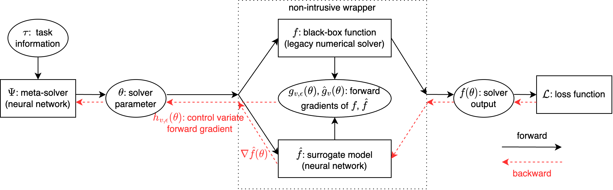
Figure 1: The overall architecture of non-intrusive gradient-based meta-solving

Algorithm 1 Non-intrusive gradient-based meta-solving

  Input: $(P,\mathcal{T})$: task space, $\Psi$: meta-solver with weight ${\bm{\omega}}$, $f$: legacy solver, $\hat{f}$: surrogate model with weight ${\bm{\phi}}$, $\mathcal{L}$: loss function, $\mathrm{Opt}$: optimizer for $\Psi$, $\hat{\mathrm{Opt}}$: optimizer for $\hat{f}$, $\hat{P}$: distribution of ${\mathbf{v}}$, $\epsilon$: positive scalar, $S$: stopping criterion

  repeat

     ${\textnormal{$\tau$}}\sim P$, ${\mathbf{v}}\sim\hat{P}$ $\rhd{}$sample task $\tau$ and random vector ${\mathbf{v}}$ from $P$ and $\hat{P}$

     Forward computation:

         ${\bm{\theta}}\leftarrow\Psi({\textnormal{$\tau$}};{\bm{\omega}})$ $\rhd{}$generate solver parameter ${\bm{\theta}}$ by $\Psi$

         $y$ $\leftarrow f({\bm{\theta}})$, $y^{+}$ $\leftarrow f({\bm{\theta}}+\epsilon{\mathbf{v}})$ $\rhd{}$solve task $\tau$ twice by $f$ using parameter ${\bm{\theta}}$ and ${\bm{\theta}}+\epsilon{\mathbf{v}}$

         $d\leftarrow\frac{y^{+}-y}{\epsilon}$ $\rhd{}$compute the directional derivative of $f$ by finite difference approximation

         $\hat{y},\hat{d}\leftarrow\mathrm{ForwardAD}(\hat{f},{\bm{\theta}},{\mathbf{v}})$ $\rhd{}$compute the output and directional derivative of $\hat{f}$ by forward mode AD

         $L\leftarrow\mathcal{L}(y)$, $\hat{L}\leftarrow(d-\hat{d})^{2}$ $\rhd{}$compute main loss $L$ and surrogate model loss $\hat{L}$

     Backward computation:

         ${\bm{h}}\leftarrow d{\mathbf{v}}-\hat{d}{\mathbf{v}}+\nabla_{\bm{\theta}}\hat{f}({\bm{\theta}})$ $\rhd{}$compute control variate forward gradient

         $\nabla_{\bm{\omega}}L\leftarrow\mathrm{ModifiedBackprop}(L,{\bm{\omega}},{\bm{h}})$ $\rhd{}$compute $\nabla_{\bm{\omega}}L$ by backpropagation while replacing $\nabla_{\bm{\theta}}f({\bm{\theta}})$ with ${\bm{h}}$

         $\nabla_{\bm{\phi}}\hat{L}\leftarrow\mathrm{Backprop}(\hat{L},{\bm{\phi}})$ $\rhd{}$compute $\nabla_{\bm{\phi}}\hat{L}$ by backpropagation

     Update:

         ${\bm{\omega}}\leftarrow\mathrm{Opt}({\bm{\omega}},\nabla_{\bm{\omega}}L)$, ${\bm{\phi}}\leftarrow\hat{\mathrm{Opt}}({\bm{\phi}},\nabla_{\bm{\phi}}\hat{L})$ $\rhd{}$update ${\bm{\omega}}$ and ${\bm{\phi}}$ by $\mathrm{Opt}$ and $\hat{\mathrm{Opt}}$ using $\nabla_{\bm{\omega}}L$ and $\nabla_{\bm{\phi}}\hat{L}$, respectively

  until $S$ is satisfied

Our non-intrusive framework can be viewed as a wrapper of a legacy numerical solver to be compatible with deep learning (Figure 1). To describe our method, we follow the meta-solving framework introduced in (Arisaka & Li, 2023). Suppose that we have task space $(\mathcal{T},P)$ and numerical solver $f$ with paramter ${\bm{\theta}}$. We want to train neural network $\Psi$ with weight ${\bm{\omega}}$, called meta-solver, to generate a good parameter ${\bm{\theta}}$ of the solver $f$ for each task $\tau\in\mathcal{T}$. The solver performance is measured by loss function $\mathcal{L}$. Then, the meta-solving problem is defined as follows:

Definition 3.1 (Meta-solving problem (Arisaka & Li, 2023)).

For a given task space $(\mathcal{T},P)$, loss function $\mathcal{L}$, solver $f$, and meta-solver $\Psi$, find ${\bm{\omega}}$ which minimizes $\mathbb{E}_{\tau\sim P}\left[\mathcal{L}(\tau,f(\tau;\Psi(\tau;{\bm{\omega}})))\right]$.

For instance, $\tau$ is to solve a linear system ${\bm{A}}{\bm{x}}={\bm{b}}$, $f$ is the Jacobi method starting from an initial guess ${\bm{\theta}}={\bm{x}}_{0}$, $\Psi$ is a neural network to generate a good initial guess ${\bm{\theta}}$ of the solver $f$ to solve $\tau$, and $\mathcal{L}$ is a surrogate of the number of iterations to converge. To train $\Psi$, Arisaka & Li (2023) proposed a gradient-based approach assuming that $\nabla f$ can be computed efficiently. However, as mentioned in Section 1, the solver $f$ in practice can be a legacy code or commercial black-box software, which does not support automatic differentiation.

To compute the gradient of legacy numerical solvers without backpropagation, we utilize the forward gradient, a low-cost estimator of the gradient.

Definition 3.2 (Forward gradient (Belouze, 2022)).

For a differentiable function $f:\mathbb{R}^{d}\to\mathbb{R}$ and a vector ${\mathbf{v}}\in\mathbb{R}^{d}$, the forward gradient ${\bm{g}}_{\mathbf{v}}:\mathbb{R}^{d}\to\mathbb{R}^{d}$ is defined as

$${\bm{g}}_{\mathbf{v}}({\bm{\theta}})=(\nabla f({\bm{\theta}})\cdot{\mathbf{v}}){\mathbf{v}}.$$ (1)

In Section 3 and Section 4, we describe and analyze our method using the definition for scalar functions, but it can be easily extended to vector-valued functions, which will be presented in Section 5. We also note that the original forward gradient is computed using forward mode automatic differentiation (Baydin et al., 2018), but we use the following finite difference approximation for legacy numerical solvers:

$${\bm{g}}_{{\mathbf{v}}}({\bm{\theta}})\approx{\bm{g}}_{{\mathbf{v}},\epsilon}({\bm{\theta}})=\frac{f({\bm{\theta}}+\epsilon{\mathbf{v}})-f({\bm{\theta}})}{\epsilon}{\mathbf{v}},$$ (2)

where $\epsilon$ is a small positive scalar.

The advantage of the forward gradient is its unbiasedness and low computational cost in terms of both time and memory. It is easily shown that if random vector ${\mathbf{v}}$’s scalar components ${\textnormal{v}}_{i}$ are independent and have zero mean and unit variance for all $i$, then the forward gradient ${\bm{g}}_{\mathbf{v}}({\bm{\theta}})$ is an unbiased estimator of $\nabla f({\bm{\theta}})$, i.e. $\mathbb{E}[{\bm{g}}_{\mathbf{v}}({\bm{\theta}})]=\nabla f({\bm{\theta}})$. As for the computational cost, the forward gradient of automatic-differentiable function $f$ such as neural networks can be computed in a single forward computation using forward mode automatic differentiation. Even if a function $f$ is implemented in legacy codes without forward mode automatic differentiation, the forward gradient can be computed using Equation 2 at the cost of evaluating $f$ twice. Note that the computation cost is equivalent to the cost of backpropagation, but it can be computed in parallel. Moreover, to compute the forward gradient, we do not need to store the intermediate values for backpropagation.

However, despite the above advantage, the practical use of the forward gradient is limited because it suffers high variance, especially in high-dimensional cases. Baydin et al. (2022) shows that the best possible variance is achieved by choosing ${\textnormal{v}}_{i}$’s to be independent Rademacher variables, i.e. $P({\textnormal{v}}_{i}=1)=P({\textnormal{v}}_{i}=-1)=1/2$ for all $i$, in which case the variance is equal to

$$\mathbb{E}[\|{\bm{g}}_{\mathbf{v}}({\bm{\theta}})-\nabla f({\bm{\theta}})\|^{2}]=(d-1)\|\nabla f({\bm{\theta}})\|^{2},$$ (3)

which is very large for large $d$. This high variance in fact hinders the training process, and we will investigate the effect of the variance in Section 4 and Section 5.

To alleviate this problem, we introduce a novel approach to reduce the variance while keeping it unbiased. The key idea is to construct control variates using a surrogate model $\hat{f}$ whose gradient $\nabla\hat{f}$ is easy to compute.

Definition 3.3 (Control variate forward gradient).

For differentiable functions $f:\mathbb{R}^{d}\to\mathbb{R}$, $\hat{f}:\mathbb{R}^{d}\to\mathbb{R}$, and a random vector ${\mathbf{v}}\in\mathbb{R}^{d}$, the control variate forward gradient ${\bm{h}}_{\mathbf{v}}:\mathbb{R}^{d}\to\mathbb{R}^{d}$ is defined as

$${\bm{h}}_{\mathbf{v}}({\bm{\theta}})={\bm{g}}_{\mathbf{v}}({\bm{\theta}})-\hat{{\bm{g}}_{\mathbf{v}}}({\bm{\theta}})+\mathbb{E}_{\mathbf{v}}[\hat{{\bm{g}}_{\mathbf{v}}}({\bm{\theta}})],$$ (4)

where $\hat{{\bm{g}}_{\mathbf{v}}}({\bm{\theta}})=(\nabla\hat{f}({\bm{\theta}})\cdot{\mathbf{v}}){\mathbf{v}}$. Similarly, we define its finite difference approximation ${\bm{h}}_{{\mathbf{v}},\epsilon}$ using ${\bm{g}}_{{\mathbf{v}},\epsilon}$ as

$${\bm{h}}_{{\mathbf{v}},\epsilon}({\bm{\theta}})={\bm{g}}_{{\mathbf{v}},\epsilon}({\bm{\theta}})-\hat{{\bm{g}}_{\mathbf{v}}}({\bm{\theta}})+\mathbb{E}_{\mathbf{v}}[\hat{{\bm{g}}_{\mathbf{v}}}({\bm{\theta}})].$$ (5)

Note that we use the finite difference approximation only for ${\bm{g}}_{\mathbf{v}}$ but not for $\hat{{\bm{g}}_{\mathbf{v}}}$ because the surrogate model $\hat{f}$ will be implemented in deep learning frameworks with automatic differentiation. The method of control variates is a classical and widely used variance reduction technique (Nelson, 1990). In the control variates method, to reduce the variance of random variable ${\mathbf{X}}$ of interest, we introduce another random variable ${\mathbf{Y}}$ which has high correlation to ${\mathbf{X}}$ and known mean $\mathbb{E}[{\mathbf{Y}}]$. Then, ${\mathbf{X}}-{\mathbf{Y}}+\mathbb{E}[{\mathbf{Y}}]$ is used as a variance-reduced estimator of ${\mathbf{X}}$. The key idea of our method is to use the forward gradient of the surrogate model $\hat{\bm{g}}_{\mathbf{v}}$ as ${\mathbf{Y}}$ so that $\mathbb{E}_{\mathbf{v}}[\hat{{\bm{g}}_{\mathbf{v}}}({\bm{\theta}})]=\nabla\hat{f}({\bm{\theta}})$ can be computed by backpropagation.

The following theorem shows that the control variate forward gradient is still unbiased under the same assumption in Belouze (2022). Furthermore, if the surrogate model $\hat{f}$ is close to the numerical solver $f$, then the control variate forward gradient ${\bm{h}}_{\mathbf{v}}$ successfully reduces the variance of the original forward gradient ${\bm{g}}_{\mathbf{v}}$.

Theorem 3.4 (Improvement by ${\bm{h}}_{\mathbf{v}}$).

If ${\textnormal{v}}_{i}$’s are independent and have zero mean and unit variance, then ${\bm{h}}_{\mathbf{v}}({\bm{\theta}})$ is an unbiased estimator of $\nabla f({\bm{\theta}})$, i.e.

$$\mathbb{E}[{\bm{h}}_{\mathbf{v}}({\bm{\theta}})]=\nabla f({\bm{\theta}}).$$ (6)

Furtheremore, if ${\textnormal{v}}_{i}$’s are independent Rademacher variables, then the mean squared deviation of ${\bm{h}}_{\mathbf{v}}({\bm{\theta}})$ is minimized and equal to

$$\mathbb{E}[\|{\bm{h}}_{\mathbf{v}}({\bm{\theta}})-\nabla f({\bm{\theta}})\|^{2}]=(d-1)\|\nabla f({\bm{\theta}})-\nabla\hat{f}({\bm{\theta}})\|^{2}.$$ (7)

The proof is found in Section A.2. Equation 7 shows the improvement from Equation 3 of the original forward gradient. In Equation 3, there is no controllable term, whereas in Equation 7, the variance can be reduced by choosing a good surrogate model $\hat{f}$. We remark that the finite difference version ${\bm{h}}_{{\mathbf{v}},\epsilon}$ is not unbiased due to ${\bm{g}}_{{\mathbf{v}},\epsilon}$ but asymptotically unbiased as $\epsilon$ tends to $0$. The error of the finite difference version is analyzed in Section A.3.

The remaining problem is how to obtain a surrogate model $\hat{f}$. To this end, we propose a novel algorithm, called Non-Intrusive Gradient-Based Meta-Solving (NI-GBMS, Algorithm 1). Its main workflow is the same as the original gradient-based meta-solving (Arisaka & Li, 2023), but it is capable of handling legacy solver $f$ whose gradient is not accessible. In NI-GBMS, we implement surrogate model $\hat{f}$ by a neural network with weight ${\bm{\phi}}$ and adaptively update it while training meta-solver $\Psi$. For training $\hat{f}$, we use

$$\hat{\mathcal{L}}({\bm{\phi}})=\left(\nabla_{\bm{\theta}}f({\bm{\theta}})\cdot{\mathbf{v}}-\nabla_{\bm{\theta}}\hat{f}({\bm{\theta}};{\bm{\phi}})\cdot{\mathbf{v}}\right)^{2}$$ (8)

as a surrogate model loss. This loss function is more suitable for our purpose than other losses that minimize the error of outputs $f({\bm{\theta}})$ and $\hat{f}({\bm{\theta}})$ (Jacovi et al., 2019). By contrast, our $\hat{\mathcal{L}}$ is designed to minimize $\|\nabla f({\bm{\theta}})-\nabla\hat{f}({\bm{\theta}})\|^{2}=\|\mathbb{E}[{{\bm{g}}_{\mathbf{v}}}({\bm{\theta}})-\hat{{\bm{g}}_{\mathbf{v}}}({\bm{\theta}})]\|^{2}$, which determines the variance of the control variate forward gradient in Equation 7. Then, the control variate forward gradient is used as an approximation of $\nabla f$ to compute $\nabla_{\bm{\omega}}\mathcal{L}$ for updating meta-solver $\Psi$.

We remark important characteristics of NI-GBMS. The most significant one is its non-intrusiveness as the name suggests. It enables us to integrate complex legacy codes and commercial black-box softwares into ML as they are. In addition, the adaptive training strategy of the surrogate model $\hat{f}$ is another advantage. By updating $\hat{f}$ during the training of meta-solver $\Psi$, it can automatically adapt to the changing distribution of ${\bm{\theta}}$ generated by the meta-solver $\Psi$. Finally, we note that the extra computational cost of training $\hat{f}$ is negligible compared to the cost of executing numerical solver $f$, which is the bottleneck of our target problem setting.

4 Analysis

To investigate the convergence property of NI-GBMS, we consider the simplest case, where a black-box solver $f$ itself is minimized over its parameter ${\bm{\theta}}$, i.e. $\min_{{\bm{\theta}}}f({\bm{\theta}})$. This is a special case of Algorithm 1, where the meta-solver $\Psi$ is a constant function that returns its parameter ${\bm{\omega}}={\bm{\theta}}$, and the loss function $\mathcal{L}$ is $f({\bm{\theta}})$ itself. This can also be considered that we directly optimize the solver parameter ${\bm{\theta}}$ for a single given task $\tau$. The optimization algorithm ${\mathrm{Opt}}$ for training $\Psi$ is a variant of the gradient descent, which uses the control variate forward gradient ${\bm{h}}_{\mathbf{v}}({\bm{\theta}})$ instead of the true gradient $\nabla f({\bm{\theta}})$, i.e. ${\bm{\theta}}_{k+1}={\bm{\theta}}_{k}-\alpha{\bm{h}}_{\mathbf{v}}({\bm{\theta}}_{k})$, where $\alpha$ is the learning rate.

4.1 Theoretical Analysis

For the considered setting, we have the following convergence theorem. Note that it is shown for the exact version of Algorithm 1, where ${\bm{h}}_{\mathbf{v}}$ is used instead of its finite difference approximation ${\bm{h}}_{{\mathbf{v}},\epsilon}$. The expectation $\mathbb{E}[\cdot]$ in the theorem is taken over all randomness of ${\mathbf{v}}$ through the training process.

Theorem 4.1 (Convergence).

Let $f:\mathbb{R}^{d}\to\mathbb{R}$ be $\mu$-strongly convex and $L$-smooth. Denote the global minimizer of $f$ by ${\bm{\theta}}_{*}$. Consider the sequence $({\bm{\theta}}_{k})_{k\in\mathbb{N}}$ and $(\hat{f}_{k})_{k\in\mathbb{N}}$ generated by NI-GBMS.

1. (No surrogate model) Suppose that $\hat{f}_{k}=\hat{f}\equiv 0$ for all $k\in\mathbb{N}$. If $\alpha\in(0,\frac{1}{Ld}]$, then the expected optimality gap satisfies the following inequality for all $k\in\mathbb{N}$:

   $$\mathbb{E}[f({\bm{\theta}}_{k})-f({\bm{\theta}}_{*})]\leq(1-\alpha\mu)^{k}(f({\bm{\theta}}_{0})-f({\bm{\theta}}_{*})).$$ (9)

2. (Fixed surrogate model) Instead of $\hat{f}\equiv 0$ in (a), suppose that $f_{k}=\hat{f}$ for all $k\in\mathbb{N}$ and $\hat{f}$ satisfies $\sup_{{\bm{\theta}}\in\mathbb{R}^{d}}\{\frac{\|\nabla f({\bm{\theta}})-\nabla\hat{f}({\bm{\theta}})\|^{2}}{\|\nabla f({\bm{\theta}})\|^{2}}\}\leq r$ for some $r\in[0,1)$. Then, we have the same inequality as Equation 9 with an improved range of learning rate $\alpha\in(0,\min\{\frac{1}{\mu},\frac{1}{Ldr}\}]$.

3. (Adaptive surrogate model) Suppose that we have

   $$\mathbb{E}[\|\nabla f({\bm{\theta}}_{k})-\nabla\hat{f}_{k}({\bm{\theta}}_{k})\|^{2}]\leq\xi^{k}\|\nabla f({\bm{\theta}}_{0})-\nabla\hat{f}_{0}({\bm{\theta}}_{0})\|^{2}$$ (10)

   for some $\xi\in(0,1)$. If $\alpha\in(0,\frac{1}{\mu}]$, then the expected optimality gap satisfies the following inequality for all $k\in\mathbb{N}$:

   $$\mathbb{E}[f({\bm{\theta}}_{k})-f({\bm{\theta}}_{*})]\leq C\rho^{k},$$ (11)

   where

   $$C=\max\{\frac{\alpha Ld\|\nabla f({\bm{\theta}}_{0})-\nabla\hat{f}_{0}({\bm{\theta}}_{0})\|^{2}}{\mu},f({\bm{\theta}}_{0})-f({\bm{\theta}}_{*})\}$$ (12)

   and

   $$\rho=\max\{1-\alpha\mu,\xi\}.$$ (13)

The proofs are presented in Section A.2. Theorem 4.1 compares our method to the original forward gradient and shows our advantage. In (a), $\hat{f}$ does nothing and the control variate forward gradient ${\bm{h}}_{\mathbf{v}}$ reduces to the original forward gradient ${\bm{g}}_{\mathbf{v}}$. This case corresponds to the original forward gradient descent (Belouze, 2022). The best convergence rate of (a) is $1-\frac{\mu}{Ld}$, which becomes worse as the dimension $d$ increases due to the increasing variance of ${\bm{g}}_{\mathbf{v}}$. The case of (b) represents the situation of having a fixed surrogate model $\hat{f}$ and shows the improvement by the control forward gradient with the surrogate model $\hat{f}$. In this case, the effective best convergence rate is $1-\frac{\mu}{Ldr}$. Although it still depends on the dimension $d$, it is improved by the factor of the relative error $r$ between $\nabla f$ and $\nabla\hat{f}$. Note that we have $\frac{1}{Ld}\leq\min\{\frac{1}{\mu},\frac{1}{Ldr}\}$ because $d\geq 1$, $r\in[0,1)$, and $\mu\leq L$ (Bottou et al., 2016). The case of (c) represents a more ideal situation where the gradient of the surrogate model $\nabla\hat{f}$ is converging to the gradient of the target function $\nabla f$ with convergence rate $\xi$. In this case, $f({\bm{\theta}}_{k})$ converges to $f({\bm{\theta}}_{*})$ with the convergence rate $\rho=\xi$, which can be independent of the dimension $d$. In summary, the convergence rate of the proposed method can be improved as the surrogate model $\hat{f}$ becomes closer to the target black-box solver $f$, and it can be independent of the dimension $d$ in the ideal case.

4.2 Numerical Experiments

Table 1: Objective values obtained using different gradient estimators. Boldface indicates the best performance except for the case of $\nabla f$.

(a) Sphere function

gradient	$d=2$	$d=8$	$d=32$	$d=128$
$\nabla f$	1.56e-12	5.88e-12	2.37e-11	9.55e-11
$\nabla\hat{f}$	9.77e-01	1.41e-02	3.67e-07	2.89e-02
${\bm{g}}_{{\mathbf{v}},\epsilon}$	1.61e-06	6.86e-03	5.88e-01	3.68e+01
${\bm{h}}_{{\mathbf{v}},\epsilon}$ (ours)	7.33e-12	8.63e-11	2.36e-09	1.36e-07

(b) Rosenbrock function

gradient	$d=2$	$d=8$	$d=32$	$d=128$
$\nabla f$	1.18e-05	5.98e-01	5.61e-01	6.06e-01
$\nabla\hat{f}$	2.23e+01	6.64e-04	7.56e-01	1.91e+02
${\bm{g}}_{{\mathbf{v}},\epsilon}$	9.06e-03	1.08e+00	1.40e+01	1.68e+02
${\bm{h}}_{{\mathbf{v}},\epsilon}$ (ours)	6.73e-04	3.40e-01	4.11e-01	7.86e-01

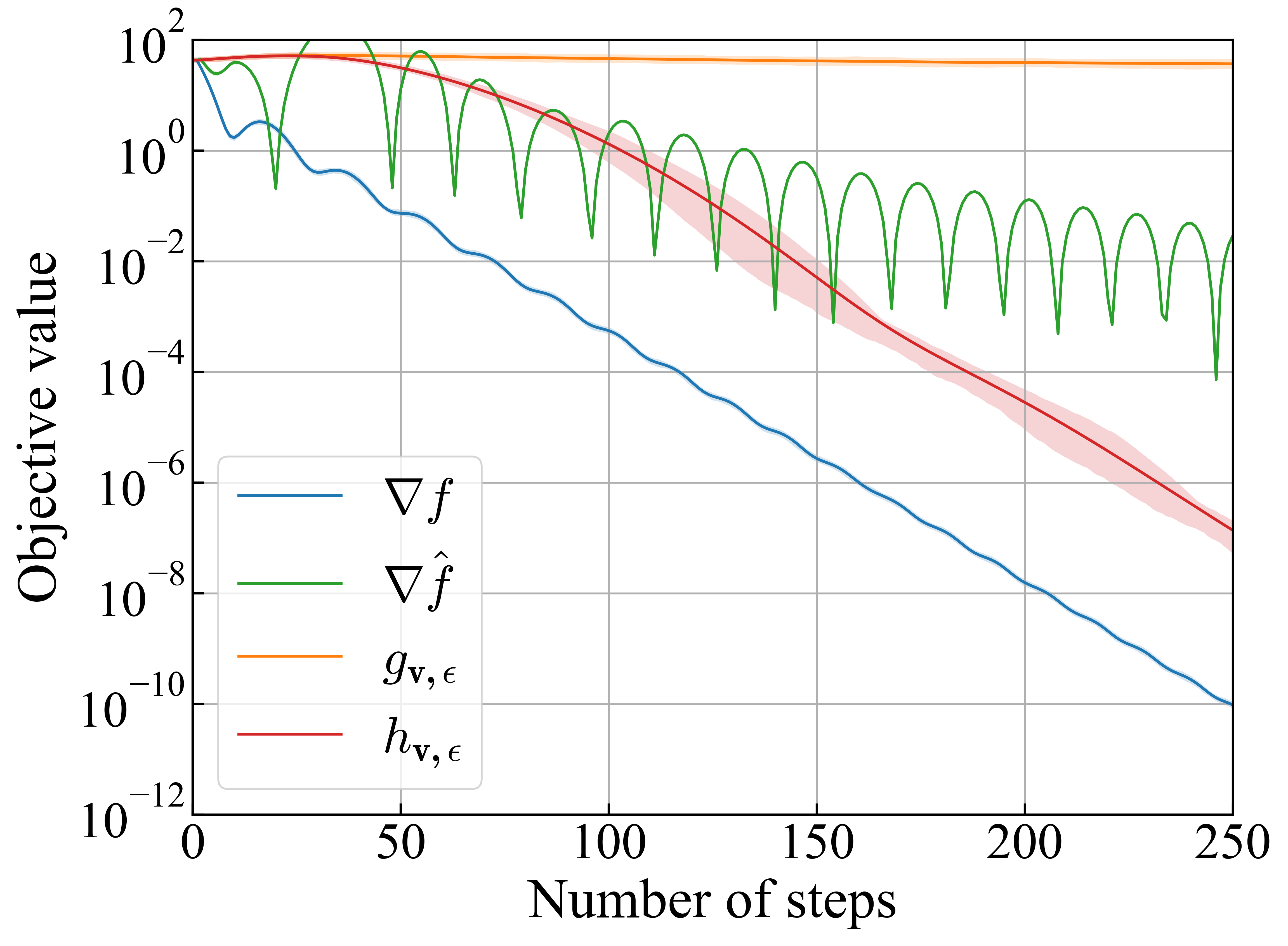
(a) The convergence plot.

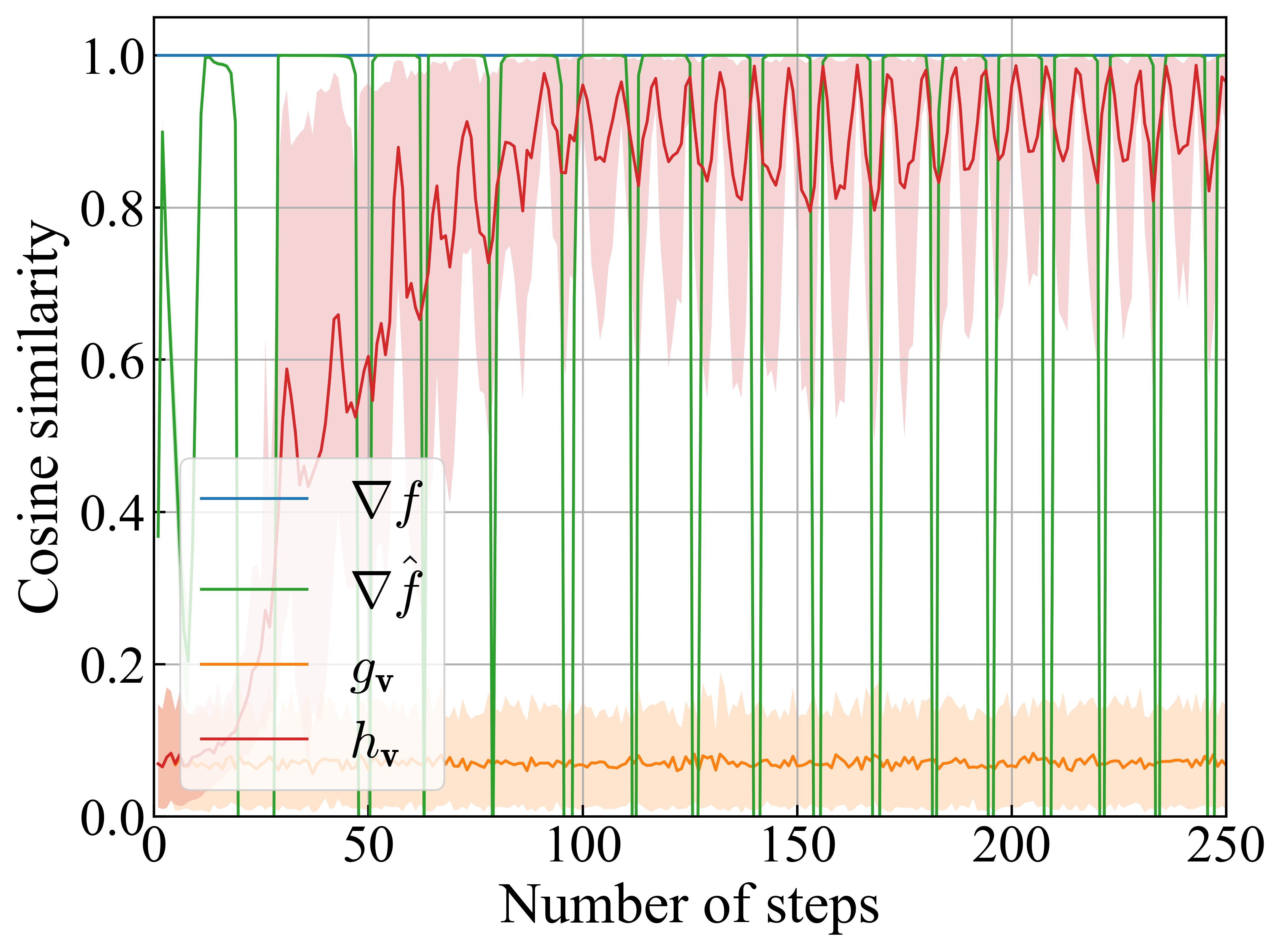
(b) Cosine similarity to the true gradient $\nabla f$.

Figure 2: The convergence plot and cosine similarity (Sphere function $d=128$). The shadowed area represents a range from 10% to 90%.

Under the same problem setting, we conduct numerical experiments using two test functions, Sphere function (Molga & Kwietnia, ):

$$f({\bm{\theta}})=\sum_{i=1}^{d}\theta_{i}^{2}$$ (14)

and Rosenbrock function (Rosenbrock, 1960):

$$f({\bm{\theta}})=\sum_{i=1}^{d-1}\left[100\left(\theta_{i+1}-\theta_{i}^{2}\right)^{2}+\left(\theta_{i}-1\right)^{2}\right]$$ (15)

with the dimension $d=2,8,32,128$. For surrogate model $\hat{f}$, we use a convolutional neural network because the relation of ${\bm{\theta}}$ coordinates is local. To update the surrogate model $\hat{f}$, the Adam optimizer (Kingma & Ba, 2015) with learning rate 0.01 is used as $\hat{\mathrm{Opt}}$. Note that the surrogate model $\hat{f}$ is trained online during minimizing $f$ without pre-training. The main optimizer ${\mathrm{Opt}}$ is also the Adam optimizer with $\alpha=0.1$ for Sphere function and $\alpha=0.01$ for the Rosenbrock function. The number of optimization steps is 250 for Sphere function and 50,000 for Rosenbrock function. For comparison, we also test using the true gradient $\nabla f$, the gradient of the surrogate model $\nabla\hat{f}$ (Jacovi et al., 2019), and the forward gradient ${\bm{g}}_{{\mathbf{v}},\epsilon}$ (Belouze, 2022) instead of our control variate forward gradient ${\bm{h}}_{{\mathbf{v}},\epsilon}$. We set finite difference step size $\epsilon=10^{-8}$. The initial parameter ${\bm{\theta}}_{0}$ is sampled from the uniform distribution on $[-1,1]^{d}$. The random vector ${\mathbf{v}}$ is sampled from the Rademacher distribution. We optimize 100 samples and report the average of their final objective values in Table 1. Other details are presented in Section A.4.

Table 1 shows the advantage of our method. For all cases including high dimensional cases, our control variate forward gradient ${\bm{h}}_{{\mathbf{v}},\epsilon}$ successfully minimize the objective function $f$ to comparable values with the best achievable baseline, the true gradient $\nabla f$. By contrast, the performance of the original forward gradient ${\bm{g}}_{{\mathbf{v}},\epsilon}$ degrades quickly as the dimension increases. The performance of the gradient of the surrogate model $\nabla\hat{f}$ is not stable. Although it can perform better than the true gradient $\nabla f$ (e.g Rosenbrock function with $d=8$) thanks to its bias, its performance is worse than our ${\bm{h}}_{{\mathbf{v}},\epsilon}$ for most cases. Figure 2 illustrates the typical behavior of each gradient estimator. In the illustrated case, the original forward gradient ${\bm{g}}_{{\mathbf{v}},\epsilon}$ fails to minimize the objective function $f$ because of its high variance, which is also shown in a low cosine similarity to the true gradient $\nabla f$ in Figure 2(b). The gradient of the surrogate model $\nabla\hat{f}$ shows unstable convergence behavior in Figure 2(a) and unstable cosine similarity in Figure 2(b). Our control variate forward gradient ${\bm{h}}_{{\mathbf{v}},\epsilon}$ resolves these undesired behaviors and shows stable convergence and high cosine similarity. Although it takes some time for the surrogate model $\hat{f}$ to fit $f$, the convergence speed after fitting is comparable to the true gradient $\nabla f$.

5 Application: Learning Parameters of Legacy Numerical Solvers

In this section, we present applications of NI-GBMS to learn good initial guesses of iterative solvers implemented in PETSc, the Portable, Extensible Toolkit for Scientific Computation (Balay et al., 2023), which is widely used for large-scale scientific applications but does not support automatic differentiation.

5.1 Toy Example: Poisson Equation

Problem setting

Let us consider solving 1D Poisson equations with different source terms repeatedly. Our task $\tau$ is to solve the 1D Poisson equation with the homogeneous Dirichlet boundary condition:

$$-\frac{d^{2}}{dz^{2}}u(z) =b_{\tau}(z),\quad z\in(0,1)$$ (16)

$$u(0) =u(1)=0.$$ (17)

Using the finite difference scheme, we discretize it to obtain the linear system ${\bm{A}}{\bm{x}}={\bm{b}}_{\tau}$, where ${\bm{A}}\in\mathbb{R}^{N\times N}$ and ${\bm{x}},{\bm{b}}_{\tau}\in\mathbb{R}^{N}$. Thus, our task $\tau$ is represented by $\tau=\{{\bm{b}}_{\tau}\}$. We use two task distributions $P$ and $Q$ described in Section A.4. The main loss function is a surrogate loss for the number of iterations $\tilde{\mathcal{L}}_{\delta}$ presented in (Arisaka & Li, 2023), which is defined recursively as:

$$\tilde{\mathcal{L}}_{\delta}^{(k+1)}(\tau;{\bm{\omega}}) =\tilde{\mathcal{L}}_{\delta}^{(k)}(\tau;{\bm{\omega}})+\sigma(\mathcal{L}_{k}(\tau;{\bm{\omega}})-\epsilon),$$ (18)

$$\tilde{\mathcal{L}}_{\delta}^{(0)}(\tau;{\bm{\omega}}) =0,$$ (19)

where $\delta$ is a given target tolerance, $\sigma$ is the sigmoid function, and $\mathcal{L}_{k}$ is the $k$-th step loss. For $\mathcal{L}_{k}$, we use the relative residual $\left\lVert{\bm{b}}_{\tau}-{\bm{A}}{\bm{x}}_{k}\right\rVert/\left\lVert{\bm{b}}_{\tau}\right\rVert$, where ${\bm{x}}_{k}$ is the solution after $k$ iterations, so the training does not require any pre-computed solutions and is conducted in a self-supervised manner. The solver $f$ is a legacy iterative solver with an initial guess ${\bm{\theta}}$ for the Poisson equation. We use the Jacobi method $f_{\textrm{Jac}}$ and the geometric multigrid method $f_{\textrm{MG}}$ (Saad, 2003) implemented in PETSc, and their tolerance $\delta$ is set to $10^{-3}$ and $10^{-8}$ respectively. The meta-solver $\Psi$ parameterized by ${\bm{\omega}}$ generates the initial guess ${\bm{\theta}}_{\tau}$ for each task $\tau$. We use a fully-connected neural network $\Psi_{\textrm{GBMS}}$ for $\Psi$. We implement surrogate model $\hat{f}$ by a fully-connected neural network. Then, we train $\Psi_{\textrm{GBMS}}$ to minimize $\tilde{\mathcal{L}}_{\delta}$ using Algorithm 1. Other details, including network architecture, the parameters of PETSc solvers, and training hyperparameters, are presented in Section A.4.

Baselines

For the purpose of comparison, we have five baselines: $\Psi_{0}$, $\Psi_{\mathrm{SL}}$, $\Psi_{\textrm{GBMS}}$ trained with $\nabla f$, $\Psi_{\textrm{GBMS}}$ trained with $\nabla\hat{f}$, and $\Psi_{\textrm{GBMS}}$ trained with ${\bm{g}}_{{\mathbf{v}},\epsilon}$. $\Psi_{0}$ is a non-learning baseline that always gives initial guess ${\bm{\theta}}=\bf{0}$, which is a reasonable choice because $u_{\tau}(0)=u_{\tau}(1)=0$ and $\mathbb{E}_{\tau\sim P}[u_{\tau}]=\mathbf{0}$. $\Psi_{\mathrm{SL}}$ is an ordinary supervised learning baseline whose network architecture is the same as $\Psi_{\mathrm{NN}}$. It is trained independently of the solver $f$ by minimizing the relative error $\left\lVert\hat{\bm{x}}-{\bm{x}}_{\tau*}\right\rVert/\left\lVert{\bm{x}}_{\tau*}\right\rVert$, where $\hat{\bm{x}}$ is the prediction of $\Psi$ and ${\bm{x}}_{\tau*}$ is the pre-computed reference solution of task $\tau$. Note that $\Psi_{\mathrm{SL}}$ does not require the gradient of the solver $f$. $\Psi_{\textrm{GBMS}}$ trained with $\nabla f$ is considered as the best achievable baseline, which is available when the solver $f$ is implemented in deep learning frameworks. $\Psi_{\textrm{GBMS}}$ trained with $\nabla\hat{f}$ is a baseline trained using the gradient of the surrogate model $\nabla\hat{f}$, which can be computed easily by backpropagation but is biased. This corresponds to the training approach proposed in Jacovi et al. (2019). $\Psi_{\textrm{GBMS}}$ trained with ${\bm{g}}_{{\mathbf{v}},\epsilon}$ is a baseline trained with the forward gradient ${\bm{g}}_{{\mathbf{v}},\epsilon}$, which is applicable to legacy solvers but suffers high variance. We also check the difference between the exact forward gradients (${\bm{g}}_{\mathbf{v}},{\bm{h}}_{\mathbf{v}}$) and the finite difference approximation (${\bm{g}}_{{\mathbf{v}},\epsilon},{\bm{h}}_{{\mathbf{v}},\epsilon}$). For training the baselines requiring automatic differentiation, we implement the Jacobi method and the geometric multigrid method using PyTorch so that they are differentiable and equivalent to the solvers in PETSc.

Results

Table 2: The average number of iterations to converge. Boldface indicates the best performance except for the case of $\nabla f$.

$\Psi$	gradient	$f=f_{\mathrm{Jac}}$	$f=f_{\mathrm{MG}}$
$\Psi_{0}$	-	173.00	90.06
$\Psi_{\mathrm{SL}}$	-	175.71	78.62
$\Psi_{\mathrm{GBMS}}$	$\nabla f$	53.64	39.29
	$\nabla\hat{f}$	106.65	52.59
	${\bm{g}}_{\mathbf{v}}$	66.76	59.06
	${\bm{g}}_{{\mathbf{v}},\epsilon}$	66.85	59.09
	${\bm{h}}_{\mathbf{v}}$	44.92	42.76
	${\bm{h}}_{{\mathbf{v}},\epsilon}$ (ours)	45.15	43.06

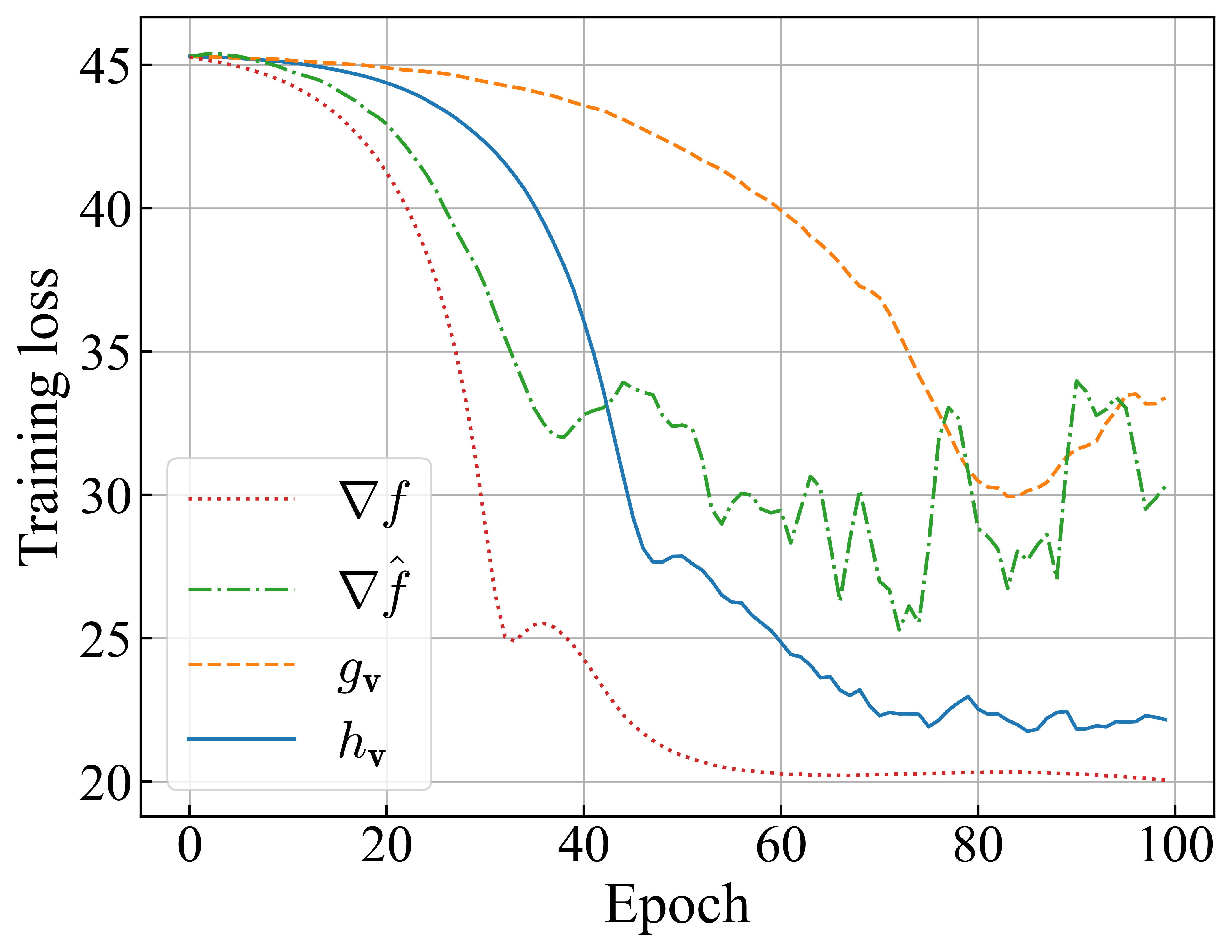
Figure 3: The learning curves of the case $f_{\mathrm{MG}}$. They are trained using a same random seed and hyperparameters except for the gradient estimator.

Table 2 presents the average number of iterations to converge starting from the initial guesses generated by each trained meta-solver. For both Jacobi and multigrid solvers, the proposed method achieves comparable results to the best achievable baseline ($\Psi_{\textrm{GBMS}}$ trained with $\nabla f$) and outperforms other baselines by a large margin. The gap between $\Psi_{\mathrm{SL}}$ and $\Psi_{\textrm{GBMS}}$ trained with $\nabla f$ shows the importance of incorporating the solver information into the training of $\Psi$ and necessity of the proposed method for legacy solvers. Table 2 also shows that there is no significant difference between the exact forward gradients and the finite difference approximation. Figure 3 shows the learning curves of the case of the multigrid method. Their behaviors are similar to the ones shown in Figure 2(a): ${\bm{g}}_{{\mathbf{v}},\epsilon}$ suffers slow training, $\nabla\hat{f}$ is unstable, and ${\bm{h}}_{{\mathbf{v}},\epsilon}$ converges similarly to $\nabla f$ after some delay for fitting $\hat{f}$. In summary, $\Psi_{\textrm{GBMS}}$ is successfully trained jointly with non-automatic-differentiable solvers using the proposed method, and reduces the number of iterations from the solver-independent supervised learning baseline $\Psi_{\mathrm{SL}}$ by 74% for the Jacobi method and 45% for the multigrid method.

5.2 Advanced Examples

To demonstrate the versatility and performance of NI-GBMS, we also consider more advanced examples, 2D biharmonic equation and 3D linear elasticity equations, using FEniCS (Alnæs et al., 2015). In these examples, we accelerate the algebraic multigrid method $f_{\mathrm{AMG}}$ in PETSc, which is one the most practical linear solvers (Stüben, 2001), by learning initial guesses using NI-GBMS. Details are presented in Section A.4.

Biharmonic Equation

The biharmonic equation is a fourth-order elliptic equation of the form: $\nabla^{4}u=b_{\tau}$ in $\Omega$, where $\nabla^{4}$ is the biharmonic operator, $\Omega$ is a domain of interest. Let $\Omega$ be $[0,1]^{2}$ and boundary conditions be $u=\nabla^{2}u=0$ on $\partial\Omega$. The source term $b_{\tau}$ is sampled from a task distribution $P$ presented in Section A.4. The equation is discretized using finite elements, and the discretized linear system is solved by the algebraic multigrid method $f_{\mathrm{AMG}}$ in PETSc.

Linear Elasticity Equations

The linear elasticity problem is described by the following equations:

$$-\nabla\cdot\sigma(u) =b_{\tau}\quad\text{ in }\Omega,$$ (20)

$$\sigma(u) =\lambda\operatorname{tr}(\epsilon(u))I+2\mu\epsilon(u)$$ (21)

$$\epsilon(u) =\frac{1}{2}\left(\nabla u+(\nabla u)^{T}\right)$$ (22)

where $\Omega=[0,1]^{3}$ is an elastic body, $u$ is the displacement field, $\sigma$ is the stress tensor, $\epsilon$ is strain-rate tensor, $\lambda$ and $\mu$ are the Lamé elasticity parameters, and $b_{\tau}$ is the body force. We consider clamped bodies deformed by their own weight by letting $u=(0,0,0)^{T}$ at $x=0$ and $b_{\tau}=(0,0,-\rho_{\tau}g)$, where $\rho_{\tau}$ is the density and $g$ is the gravitational acceleration. The density $\rho_{\tau}$ is sampled from the log uniform distribution on $[10^{-2},10^{2}]$, which determines our task space. Then, the equations are discretized using finite elements and solved by $f_{\mathrm{AMG}}$.

Results

The performance improvement by NI-GBMS is shown in Table 3, where the average number of iterations is reduced from the default initial guess, which is the zero vector, by 57% for the biharmonic equation and 71% for the linear elasticity equations. This result demonstrates the versatility and performance of NI-GBMS for more advanced problem settings.

Table 3: The average number of iterations to reach relative residual tolerance $\delta=10^{-5}$.

	Biharmonic Eq.	Elasticity Eq.
Default PETSc	73.74	88.71
Enhanced by NI-GBMS	31.54	25.61

6 Conclusion

In this paper, we proposed NI-GBMS, a novel methodology to combine meta-solvers parametrized by neural networks and non-automatic-differentiable legacy solvers without any modification. To develop this, we introduced the control variate forward gradient, which is unbiased and has lower variance than the original forward gradient. Furthermore, we proposed a practical algorithm to construct the control variate forward gradient using an adaptive surrogate model. It was theoretically and numerically shown that the proposed method has better convergence property than other baselines. We applied NI-GBMS to learn initial guesses of established iterative solvers in PETSc, resulting in a significant reduction of the number of iterations to converge. Our proposed method expands the range of applications of neural networks, and it can be a fundamental building block to combine modern neural networks and legacy numerical solvers.

In future work, we will explore more sophisticated architectures of the surrogate model, which can leverage our prior knowledge of the solver and problem and lead to better performance. For example, one can build surrogate model $\hat{f}=\hat{f}_{2}\circ\hat{f}_{1}$ using two building blocks $\hat{f}_{1}$ and $\hat{f}_{2}$, where $\hat{f}_{1}$ is the same algorithm as legacy solver $f$ but implemented in a deep learning framework and working on a smaller problem size, and $\hat{f}_{2}$ is a neural network to correct the difference between $f$ and $\hat{f}_{1}$. Beyond scientific computing applications, our proposed method can be useful to the problems of learning to optimize (Chen et al., 2021), where memory limitation often becomes a practical bottleneck because the computation graph tends to be too large for backpropagation. We expect that this limitation can be overcome by the proposed method using the high-quality gradient estimation without storing intermediate values.

Impact Statements

This paper presents work whose goal is to advance the field of Machine Learning. There are many potential societal consequences of our work, none which we feel must be specifically highlighted here.

Appendix A Appendix

A.1 implementation

The source code of the experiments is available at https://github.com/icml2024paper/NI-GBMS.

A.2 Proofs

Proof of Theorem 3.4.

To lighten the notation, we omit ${\bm{\theta}}$ dependence. Denoting $i$th component of ${\bm{g}}_{\mathbf{v}}$ by ${g_{{\mathbf{v}}}}_{i}$,

$$\mathbb{E}[{{g_{{\mathbf{v}}}}_{i}}^{2}] =\mathbb{E}\left[(\nabla f\cdot{\mathbf{v}})^{2}{\textnormal{v}}_{i}^{2}\right]$$ (23)

$$=\mathbb{E}\left[\left(\frac{\partial f}{\partial\theta_{i}}\right)^{2}{{\textnormal{v}}_{i}}^{4}+\sum_{j\neq i}\left(\frac{\partial f}{\partial\theta_{j}}\right)^{2}{{\textnormal{v}}_{i}}^{2}{{\textnormal{v}}_{j}}^{2}+2\sum_{k<l}\frac{\partial f}{\partial\theta_{k}}\frac{\partial f}{\partial\theta_{l}}{{\textnormal{v}}_{i}}^{2}{\textnormal{v}}_{k}{\textnormal{v}}_{l}\right]$$ (24)

$$=\left(\frac{\partial f}{\partial\theta_{i}}\right)^{2}\mathbb{E}[{{\textnormal{v}}_{i}}^{4}]+\sum_{j\neq i}\left(\frac{\partial f}{\partial\theta_{j}}\right)^{2}\mathbb{E}[{{\textnormal{v}}_{i}}^{2}]\mathbb{E}[{{\textnormal{v}}_{j}}^{2}]+2\sum_{k<l}\frac{\partial f}{\partial\theta_{k}}\frac{\partial f}{\partial\theta_{l}}\mathbb{E}[{{\textnormal{v}}_{i}}^{2}]\mathbb{E}[{\textnormal{v}}_{k}]\mathbb{E}[{\textnormal{v}}_{l}]$$ (25)

$$=\left(\frac{\partial f}{\partial\theta_{i}}\right)^{2}(1+\mathrm{Var}[{{\textnormal{v}}_{i}}^{2}])+\sum_{j\neq i}\left(\frac{\partial f}{\partial\theta_{j}}\right)^{2}$$ (26)

$$=\left(\frac{\partial f}{\partial\theta_{i}}\right)^{2}\mathrm{Var}[{{\textnormal{v}}_{i}}^{2}]+\|\nabla f\|^{2}.$$ (27)

Hence,

$$\mathbb{E}[{{h_{{\mathbf{v}}}}_{i}}^{2}] =\mathbb{E}\left[\left({g_{{\mathbf{v}}}}_{i}-\hat{g_{\mathbf{v}}}_{i}+\mathbb{E}[\hat{g_{\mathbf{v}}}_{i}]\right)^{2}\right]$$ (28)

$$=\mathbb{E}\left[\left((\nabla f\cdot{\mathbf{v}}){\textnormal{v}}_{i}-(\nabla\hat{f}\cdot{\mathbf{v}}){\textnormal{v}}_{i}+\frac{\partial\hat{f}}{\partial\theta_{i}}\right)^{2}\right]$$ (29)

$$=\mathbb{E}\left[\left((\nabla f-\nabla\hat{f})\cdot{\mathbf{v}}){\textnormal{v}}_{i}+\frac{\partial\hat{f}}{\partial\theta_{i}}\right)^{2}\right]$$ (30)

$$=\mathbb{E}\left[\left((\nabla f-\nabla\hat{f})\cdot{\mathbf{v}}\right)^{2}{\textnormal{v}}_{i}^{2}+2\left((\nabla f-\nabla\hat{f})\cdot{\mathbf{v}}\right){\textnormal{v}}_{i}\frac{\partial\hat{f}}{\partial\theta_{i}}+\left(\frac{\partial\hat{f}}{\partial\theta_{i}}\right)^{2}\right]$$ (31)

$$=\mathbb{E}\left[\left((\nabla f-\nabla\hat{f})\cdot{\mathbf{v}}\right)^{2}{\textnormal{v}}_{i}^{2}\right]+2\mathbb{E}\left[((\nabla f-\nabla\hat{f})\cdot{\mathbf{v}}){\textnormal{v}}_{i}\right]\frac{\partial\hat{f}}{\partial\theta_{i}}+\left(\frac{\partial\hat{f}}{\partial\theta_{i}}\right)^{2}$$ (32)

$$=\left(\frac{\partial f}{\partial\theta_{i}}-\frac{\partial\hat{f}}{\partial\theta_{i}}\right)^{2}\mathrm{Var}[{{\textnormal{v}}_{i}}^{2}]+\|\nabla f-\nabla\hat{f}\|^{2}+2\left(\frac{\partial f}{\partial\theta_{i}}-\frac{\partial\hat{f}}{\partial\theta_{i}}\right)\frac{\partial\hat{f}}{\partial\theta_{i}}+\left(\frac{\partial\hat{f}}{\partial\theta_{i}}\right)^{2}$$ (33)

$$=\left(\frac{\partial f}{\partial\theta_{i}}-\frac{\partial\hat{f}}{\partial\theta_{i}}\right)^{2}\mathrm{Var}[{{\textnormal{v}}_{i}}^{2}]+\|\nabla f-\nabla\hat{f}\|^{2}+2\frac{\partial f}{\partial\theta_{i}}\frac{\partial\hat{f}}{\partial\theta_{i}}-\left(\frac{\partial\hat{f}}{\partial\theta_{i}}\right)^{2}.$$ (34)

Therefore,

$$\mathbb{E}[\|{\bm{h}}_{\mathbf{v}}-\nabla f\|^{2}]$$ (35)

$$= \mathbb{E}[\|{\bm{h}}_{\mathbf{v}}\|^{2}]-\|\nabla f\|^{2}$$ (36)

$$= \sum_{i=1}^{d}\mathbb{E}[{{h_{{\mathbf{v}}}}_{i}}^{2}]-\|\nabla f\|^{2}$$ (37)

$$= \sum_{i=1}^{d}\left(\frac{\partial f}{\partial\theta_{i}}-\frac{\partial\hat{f}}{\partial\theta_{i}}\right)^{2}\mathrm{Var}[{{\textnormal{v}}_{i}}^{2}]+d\|\nabla f-\nabla\hat{f}\|^{2}+2\nabla f\cdot\nabla\hat{f}-\|\nabla\hat{f}\|^{2}-\|\nabla f\|^{2}$$ (38)

$$= \sum_{i=1}^{d}\left(\frac{\partial f}{\partial\theta_{i}}-\frac{\partial\hat{f}}{\partial\theta_{i}}\right)^{2}\mathrm{Var}[{{\textnormal{v}}_{i}}^{2}]+(d-1)\|\nabla f-\nabla\hat{f}\|^{2}$$ (39)

This is minimized when $\mathrm{Var}[{{\textnormal{v}}_{i}}^{2}]=0$ for all $i$, which implies ${\textnormal{v}}_{i}$’s are independent Rademacher variables. Then, the minimized deviation is

$$\mathbb{E}[\|{\bm{h}}_{\mathbf{v}}-\nabla f\|^{2}]=(d-1)\|\nabla f-\nabla\hat{f}\|^{2}.$$ (40)

∎

Proof of Theorem 4.1.

To prove Theorem 4.1, we introduce Lemma A.1 and Lemma A.2.

Lemma A.1.

If $f:\mathbb{R}^{d}\to\mathbb{R}$ is $L$-smooth, then for all $k\in\mathbb{N}$, we have

$$\mathbb{E}[f({\bm{\theta}}_{k+1})]-f({\bm{\theta}}_{k})\leq-\alpha\|\nabla f({\bm{\theta}}_{k})\|^{2}+\frac{\alpha^{2}Ld}{2}\|\nabla f({\bm{\theta}}_{k})-\nabla\hat{f}_{k}({\bm{\theta}}_{k})\|^{2}.$$ (41)

Proof.

Since $f$ is $L$-smooth, we have

$$f({\bm{\theta}}_{k+1})-f({\bm{\theta}}_{k}) \leq\nabla f({\bm{\theta}}_{k})\cdot({\bm{\theta}}_{k+1}-{\bm{\theta}}_{k})+\frac{L}{2}\|{\bm{\theta}}_{k+1}-{\bm{\theta}}_{k}\|$$ (42)

$$=\alpha\nabla f({\bm{\theta}}_{k})\cdot{\bm{h}}_{\mathbf{v}}({\bm{\theta}}_{k})+\frac{\alpha^{2}L}{2}\|{\bm{h}}_{\mathbf{v}}({\bm{\theta}}_{k})\|$$ (43)

Then, taking expectations with respect to ${\mathbf{v}}$ at the $k$th step and using Equation 6 and Equation 7, we have the desired inequality. ∎

Lemma A.2 (Polyak (1963)).

$\mu$-strong convexity implies $\mu$-Polyak-Łojasiewicz inequality:

$$2\mu(f({\bm{\theta}})-f({\bm{\theta}}_{*}))\leq\|\nabla f({\bm{\theta}})\|^{2}$$ (44)

Proof.

The proof can be found in Bottou et al. (2016). ∎

Now let us prove Theorem 4.1.

1. When $\hat{f}_{k}\equiv 0$, Equation 41 reduces to

   $$\mathbb{E}[f({\bm{\theta}}_{k+1})]-f({\bm{\theta}}_{k}) \leq-\alpha\|\nabla f({\bm{\theta}}_{k})\|^{2}+\frac{\alpha^{2}Ld}{2}\|\nabla f({\bm{\theta}}_{k})\|^{2}$$ (45)

   $$=-\alpha(1-\frac{\alpha Ld}{2})\|\nabla f({\bm{\theta}}_{k})\|^{2}$$ (46)

   $$\leq-\frac{\alpha}{2}\|\nabla f({\bm{\theta}}_{k})\|^{2}$$ (47)

   $$\leq-\alpha\mu(f({\bm{\theta}}_{k})-f({\bm{\theta}}_{*})).$$ (48)

   Subtracting $f({\bm{\theta}}_{*})$, taking total expectations, and rearranging, this yields

   $$\mathbb{E}[f({\bm{\theta}}_{k+1})-f({\bm{\theta}}_{*})]\leq(1-\alpha\mu)\mathbb{E}[f({\bm{\theta}}_{k})-f({\bm{\theta}}_{*})].$$ (49)

   By applying this inequality repeatedly, the desired inequality follows.

2. When $\sup_{{\bm{\theta}}\in\mathbb{R}^{d}}\{\frac{\|\nabla f({\bm{\theta}})-\nabla\hat{f}({\bm{\theta}})\|^{2}}{\|\nabla f({\bm{\theta}})\|^{2}}\}\leq r$, Equation 41 reduces to

   $$\mathbb{E}[f({\bm{\theta}}_{k+1})]-f({\bm{\theta}}_{k})\leq-\alpha\|\nabla f({\bm{\theta}}_{k})\|^{2}+\frac{\alpha^{2}Ldr}{2}\|\nabla f({\bm{\theta}}_{k})\|^{2}.$$ (50)

   Then, the rest of the proof is the same as (a)

3. By Lemma A.2, Equation 41 gives

   $$\mathbb{E}[f({\bm{\theta}}_{k+1})]-f({\bm{\theta}}_{k})\leq-2\alpha\mu(f({\bm{\theta}}_{k})-f({\bm{\theta}}_{*}))+\frac{\alpha^{2}Ld}{2}\|\nabla f({\bm{\theta}}_{k})-\nabla\hat{f}_{k}({\bm{\theta}}_{k})\|^{2}.$$ (51)

   Subtracting $f({\bm{\theta}}_{*})$, taking total expectations, and rearranging, this yields

   $$\mathbb{E}[f({\bm{\theta}}_{k+1})-f({\bm{\theta}}_{*})]\leq(1-2\alpha\mu)\mathbb{E}[f({\bm{\theta}}_{k})-f({\bm{\theta}}_{*})]+\frac{\alpha^{2}Ld}{2}\mathbb{E}[\|\nabla f({\bm{\theta}}_{k})-\nabla\hat{f}_{k}({\bm{\theta}}_{k})\|^{2}].$$ (52)

   Using the assumption Equation 10, we have

   $$\mathbb{E}[f({\bm{\theta}}_{k+1})-f({\bm{\theta}}_{*})] \leq(1-2\alpha\mu)\mathbb{E}[f({\bm{\theta}}_{k})-f({\bm{\theta}}_{*})]+\frac{\alpha^{2}Ldr}{2}\xi^{k}\|\nabla f({\bm{\theta}}_{0})-\nabla\hat{f}_{0}({\bm{\theta}}_{0})\|^{2}$$ (53)

   $$\leq(1-2\alpha\mu)\mathbb{E}[f({\bm{\theta}}_{k})-f({\bm{\theta}}_{*})]+\alpha\mu C\xi^{k},$$ (54)

   where

   $$C=\max\{\frac{\alpha Ld\|\nabla f({\bm{\theta}}_{0})-\nabla\hat{f}_{0}({\bm{\theta}}_{0})\|^{2}}{\mu},f({\bm{\theta}}_{0})-f({\bm{\theta}}_{*})\}.$$ (55)

   Using this inequality, we prove Equation 11 by induction. For $k=0$, we have

   $$\mathbb{E}[f({\bm{\theta}}_{1})-f({\bm{\theta}}_{*})] \leq(1-2\alpha\mu)(f({\bm{\theta}}_{0})-f({\bm{\theta}}_{*}))+\alpha\mu C$$ (56)

   $$\leq\rho C.$$ (57)

   Assume Equation 11 holds for $k$. Then, we have

   $$\mathbb{E}[f({\bm{\theta}}_{k+1})-f({\bm{\theta}}_{*})] \leq(1-2\alpha\mu)C\rho^{k}+\alpha\mu C\xi^{k}$$ (58)

   $$\leq C\rho^{k}\left(1-2\alpha\mu+\alpha\mu\left(\frac{\xi}{\rho}\right)^{k}\right)$$ (59)

   $$\leq C\rho^{k}\left(1-2\alpha\mu+\alpha\mu\right)$$ (60)

   $$\leq C\rho^{k+1}.$$ (61)

∎

A.3 Analysis for the finite difference approximation

Theorem A.3.

Let ${\textnormal{v}}_{i}$’s be independent Rademacher variables and $f:\mathbb{R}^{d}\to\mathbb{R}$ be $L$-smooth. Then, we have the following bounds for the control variate forward gradient ${\bm{h}}_{{\mathbf{v}},\epsilon}({\bm{\theta}})$ for all ${\bm{\theta}}\in\mathbb{R}^{d}$:

$$\left\lVert\mathbb{E}[{\bm{h}}_{{\mathbf{v}},\epsilon}({\bm{\theta}})]-\nabla f({\bm{\theta}})\right\rVert\leq\frac{\epsilon Ld^{3/2}}{2},$$ (62)

and

$$\mathbb{E}[\left\lVert{\bm{h}}_{{\mathbf{v}},\epsilon}({\bm{\theta}})-\nabla f({\bm{\theta}})\right\rVert^{2}]\leq\frac{\epsilon^{2}L^{2}d^{3}}{4}+2(d-1)\frac{\epsilon Ld^{3/2}}{2}\left\lVert\nabla f({\bm{\theta}})-\nabla\hat{f}({\bm{\theta}})\right\rVert+(d-1)\left\lVert\nabla f({\bm{\theta}})-\nabla\hat{f}({\bm{\theta}})\right\rVert^{2}\\$$ (63)

Proof.

Since $f$ is $L$-smooth, we have

$$\lvert f({\bm{x}})-f({\bm{y}})-\nabla f({\bm{y}})\cdot({\bm{x}}-{\bm{y}})\rvert\leq\frac{L}{2}\left\lVert{\bm{x}}-{\bm{y}}\right\rVert^{2}\quad(\forall{\bm{x}},{\bm{y}}\in\mathbb{R}^{d}).$$ (64)

This inequality with ${\bm{\theta}}+\epsilon{\mathbf{v}}$ and ${\bm{\theta}}$ yields

$$\lvert f({\bm{\theta}}+\epsilon{\mathbf{v}})-f({\bm{\theta}})-\nabla f({\bm{\theta}})\cdot\epsilon{\mathbf{v}}\rvert \leq\frac{L}{2}\left\lVert\epsilon{\mathbf{v}}\right\rVert^{2}$$ (65)

$$=\frac{\epsilon^{2}Ld}{2}.$$ (66)

We denote $D_{{\mathbf{v}},\epsilon}({\bm{\theta}}):=\frac{f({\bm{\theta}}+\epsilon{\mathbf{v}})-f({\bm{\theta}})}{\epsilon}-\nabla f({\bm{\theta}})\cdot{\mathbf{v}}$. Note that $\lvert D_{{\mathbf{v}},\epsilon}({\bm{\theta}})\rvert\leq\epsilon Ld/2$. Using this inequality, we can show inequality (62) as follows:

$$\left\lVert\mathbb{E}[{\bm{h}}_{{\mathbf{v}},\epsilon}({\bm{\theta}})]-\nabla f({\bm{\theta}})\right\rVert =\left\lVert\mathbb{E}[{\bm{g}}_{{\mathbf{v}},\epsilon}({\bm{\theta}})-\hat{{\bm{g}}_{\mathbf{v}}}({\bm{\theta}})+\mathbb{E}[\hat{{\bm{g}}_{\mathbf{v}}}({\bm{\theta}})]]-\mathbb{E}[{\bm{g}}_{\mathbf{v}}({\bm{\theta}})]\right\rVert$$ (67)

$$=\left\lVert\mathbb{E}[{\bm{g}}_{{\mathbf{v}},\epsilon}({\bm{\theta}})-{{\bm{g}}_{\mathbf{v}}}({\bm{\theta}})]\right\rVert$$ (68)

$$\leq\mathbb{E}[\left\lVert{\bm{g}}_{{\mathbf{v}},\epsilon}({\bm{\theta}})-{{\bm{g}}_{\mathbf{v}}}({\bm{\theta}})\right\rVert]$$ (69)

$$=\mathbb{E}[\left\lVert\frac{f({\bm{\theta}}+\epsilon{\mathbf{v}})-f({\bm{\theta}})}{\epsilon}{\mathbf{v}}-(\nabla f({\bm{\theta}})\cdot{\mathbf{v}}){\mathbf{v}}\right\rVert]$$ (70)

$$=\mathbb{E}[\lvert D_{{\mathbf{v}},\epsilon}({\bm{\theta}})\rvert\left\lVert{\mathbf{v}}\right\rVert]$$ (71)

$$\leq\frac{\epsilon Ld}{2}d^{1/2}$$ (72)

$$=\frac{\epsilon Ld^{3/2}}{2}.$$ (73)

Next, we show inequality (63). To simplify the notation, we omit the argument ${\bm{\theta}}$. Then, we have

$$\mathbb{E}[\left\lVert{\bm{h}}_{{\mathbf{v}},\epsilon}-\nabla f\right\rVert^{2}] =\mathbb{E}[\left\lVert({\bm{g}}_{{\mathbf{v}},\epsilon}-{\bm{g}}_{\mathbf{v}})+({\bm{h}}_{\mathbf{v}}-\nabla f)\right\rVert^{2}]$$ (74)

$$=\mathbb{E}[\left\lVert D_{{\mathbf{v}},\epsilon}{\mathbf{v}}+({\bm{h}}_{\mathbf{v}}-\nabla f)\right\rVert^{2}]$$ (75)

$$=\mathbb{E}[\left\lVert D_{{\mathbf{v}},\epsilon}{\mathbf{v}}\right\rVert^{2}]+2\mathbb{E}[D_{{\mathbf{v}},\epsilon}{\mathbf{v}}\cdot({\bm{h}}_{\mathbf{v}}-\nabla f)]+\mathbb{E}[\left\lVert{\bm{h}}_{\mathbf{v}}-\nabla f\right\rVert^{2}]$$ (76)

$$=\mathbb{E}[{D_{{\mathbf{v}},\epsilon}}^{2}\left\lVert{\mathbf{v}}\right\rVert^{2}]+2\mathbb{E}[D_{{\mathbf{v}},\epsilon}{\mathbf{v}}\cdot({\bm{g}}_{\mathbf{v}}-\hat{\bm{g}}_{\mathbf{v}}+\nabla\hat{f}-\nabla f)]+(d-1)\left\lVert\nabla f-\nabla\hat{f}\right\rVert^{2}$$ (77)

$$=\mathbb{E}[{D_{{\mathbf{v}},\epsilon}}^{2}\left\lVert{\mathbf{v}}\right\rVert^{2}]+2\mathbb{E}[D_{{\mathbf{v}},\epsilon}{\mathbf{v}}\cdot({\bm{g}}_{\mathbf{v}}-\hat{\bm{g}}_{\mathbf{v}})]+2\mathbb{E}[D_{{\mathbf{v}},\epsilon}{\mathbf{v}}]\cdot(\nabla\hat{f}-\nabla f)+(d-1)\left\lVert\nabla f-\nabla\hat{f}\right\rVert^{2}$$ (78)

$$=\mathbb{E}[{D_{{\mathbf{v}},\epsilon}}^{2}\left\lVert{\mathbf{v}}\right\rVert^{2}]+2\mathbb{E}[D_{{\mathbf{v}},\epsilon}{\mathbf{v}}\cdot((\nabla f-\nabla\hat{f})\cdot{\mathbf{v}}){\mathbf{v}}]+2\mathbb{E}[D_{{\mathbf{v}},\epsilon}{\mathbf{v}}]\cdot(\nabla\hat{f}-\nabla f)+(d-1)\left\lVert\nabla f-\nabla\hat{f}\right\rVert^{2}$$ (79)

$$=\mathbb{E}[{D_{{\mathbf{v}},\epsilon}}^{2}\left\lVert{\mathbf{v}}\right\rVert^{2}]+2\mathbb{E}[D_{{\mathbf{v}},\epsilon}((\nabla f-\nabla\hat{f})\cdot{\mathbf{v}})\left\lVert{\mathbf{v}}\right\rVert^{2}]+2\mathbb{E}[D_{{\mathbf{v}},\epsilon}{\mathbf{v}}]\cdot(\nabla\hat{f}-\nabla f)+(d-1)\left\lVert\nabla f-\nabla\hat{f}\right\rVert^{2}$$ (80)

$$=d\mathbb{E}[{D_{{\mathbf{v}},\epsilon}}^{2}]+2d\mathbb{E}[D_{{\mathbf{v}},\epsilon}((\nabla f-\nabla\hat{f})\cdot{\mathbf{v}})]+2\mathbb{E}[D_{{\mathbf{v}},\epsilon}{\mathbf{v}}]\cdot(\nabla\hat{f}-\nabla f)+(d-1)\left\lVert\nabla f-\nabla\hat{f}\right\rVert^{2}$$ (81)

$$=d\mathbb{E}[{D_{{\mathbf{v}},\epsilon}}^{2}]+2(d-1)\mathbb{E}[D_{{\mathbf{v}},\epsilon}{\mathbf{v}}]\cdot(\nabla f-\nabla\hat{f})+(d-1)\left\lVert\nabla f-\nabla\hat{f}\right\rVert^{2}$$ (82)

$$\leq d(\frac{\epsilon Ld}{2})^{2}+2(d-1)\frac{\epsilon Ld^{3/2}}{2}\left\lVert\nabla f-\nabla\hat{f}\right\rVert+(d-1)\left\lVert\nabla f-\nabla\hat{f}\right\rVert^{2}$$ (83)

$$=\frac{\epsilon^{2}L^{2}d^{3}}{4}+2(d-1)\frac{\epsilon Ld^{3/2}}{2}\left\lVert\nabla f-\nabla\hat{f}\right\rVert+(d-1)\left\lVert\nabla f-\nabla\hat{f}\right\rVert^{2}.$$ (84)

∎

A.4 Details of numerical examples

A.4.1 Details of Section 4.2

Surrogate model

In Section 4.2, our surrogate model $\hat{f}$ has two convlutional layers with 64 filters, followed by a global average pooling and a fully connected layer with 64 units. The kernel size is 1 for the Sphere function and 3 for the Rosenbrock function. The activation function is GELU (Hendrycks & Gimpel, 2016).

Results

The standard deviation of the objective values are presented in Table 4, and convergence plots are shown in Figure 4.

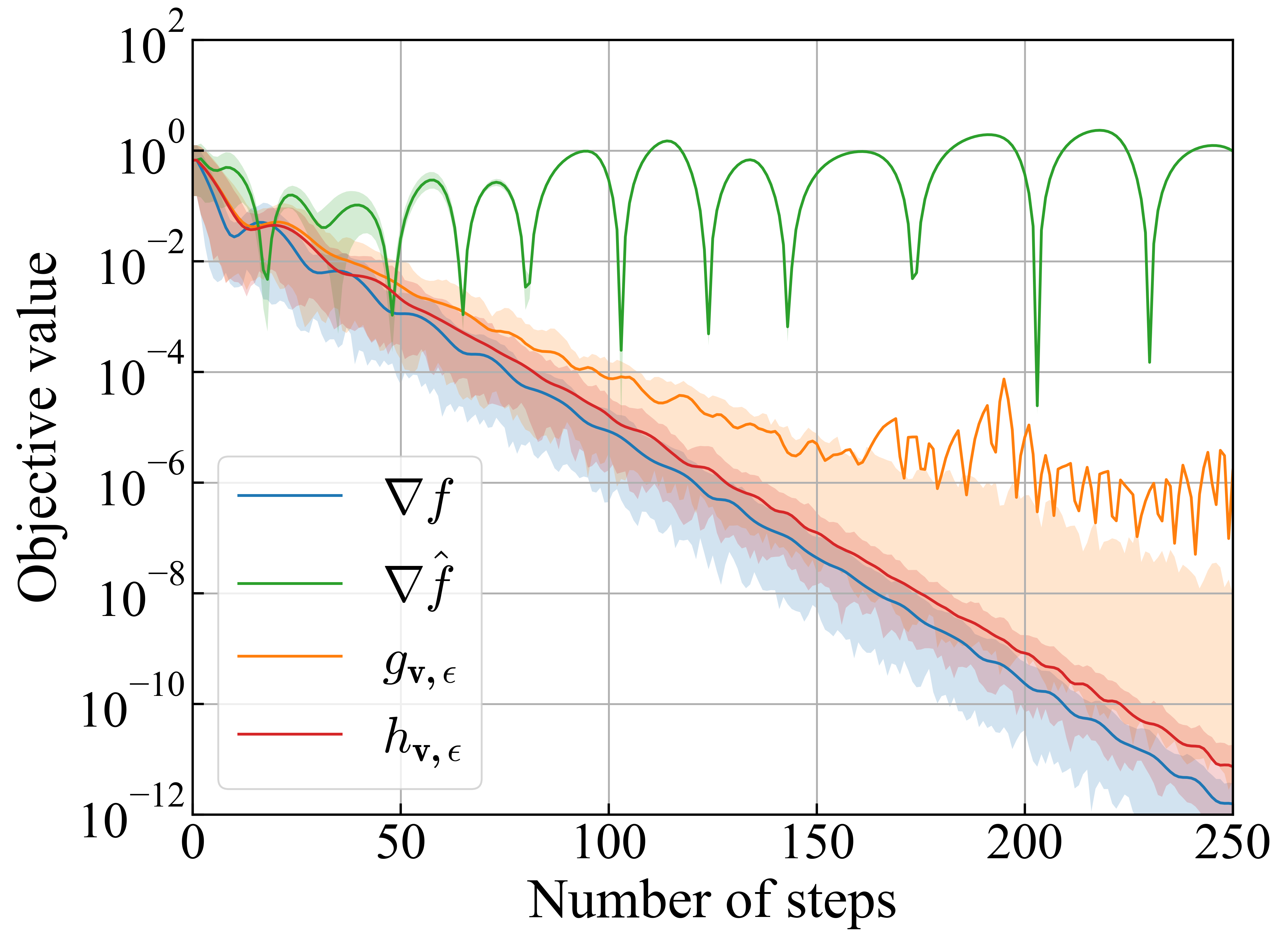
(a) sphere2D

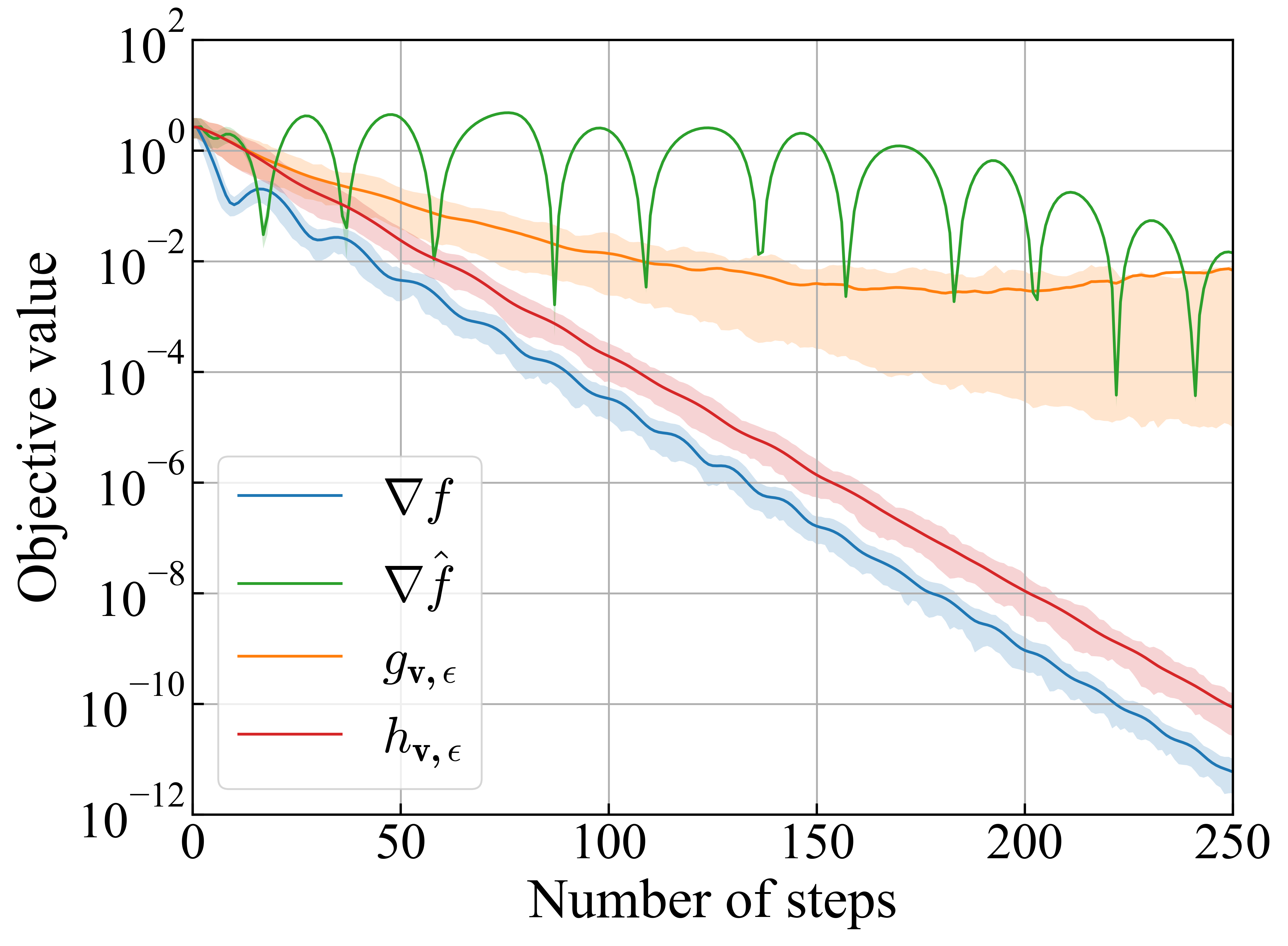
(b) sphere8D

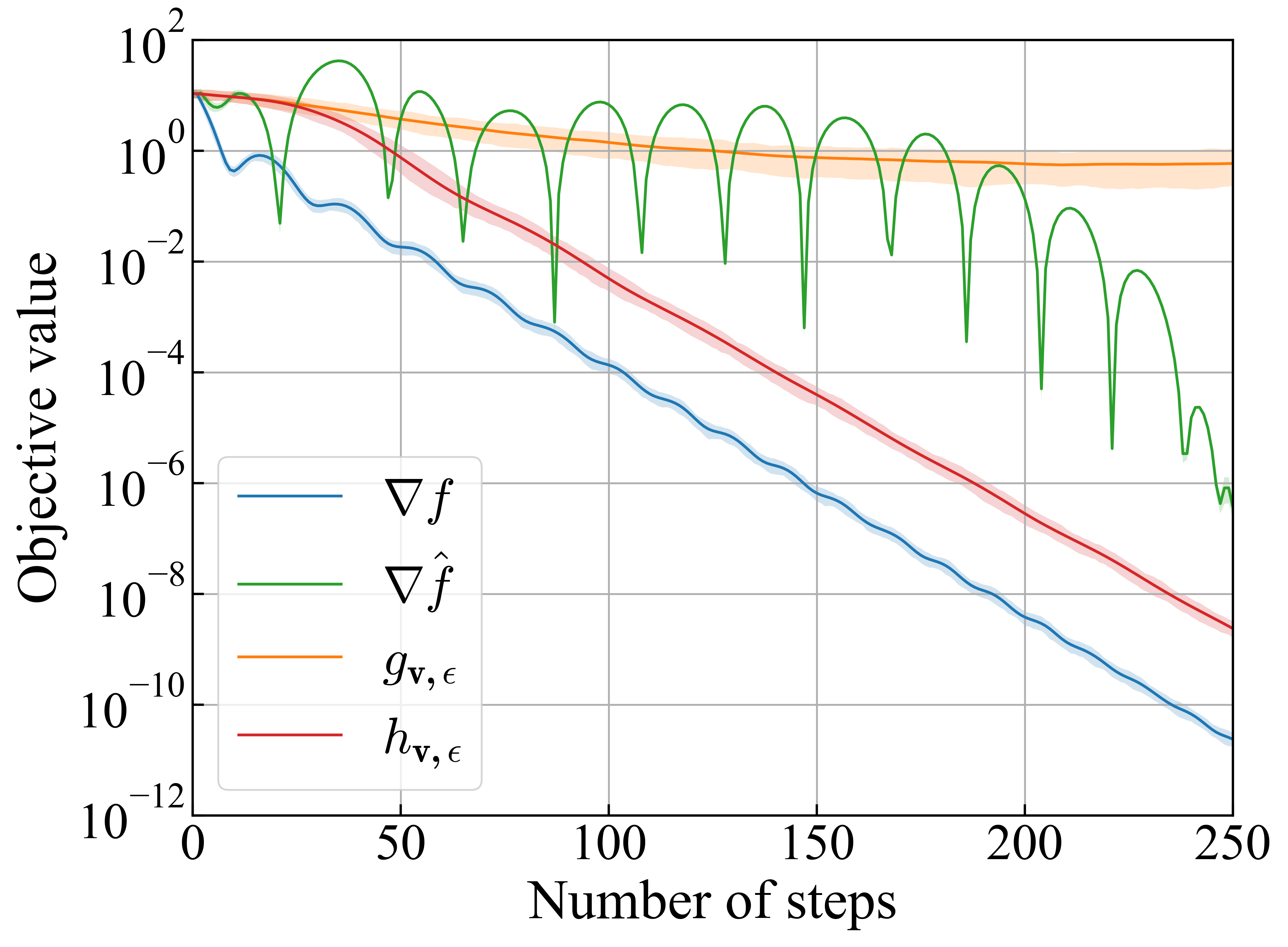
(c) sphere32D

(d) sphere128D

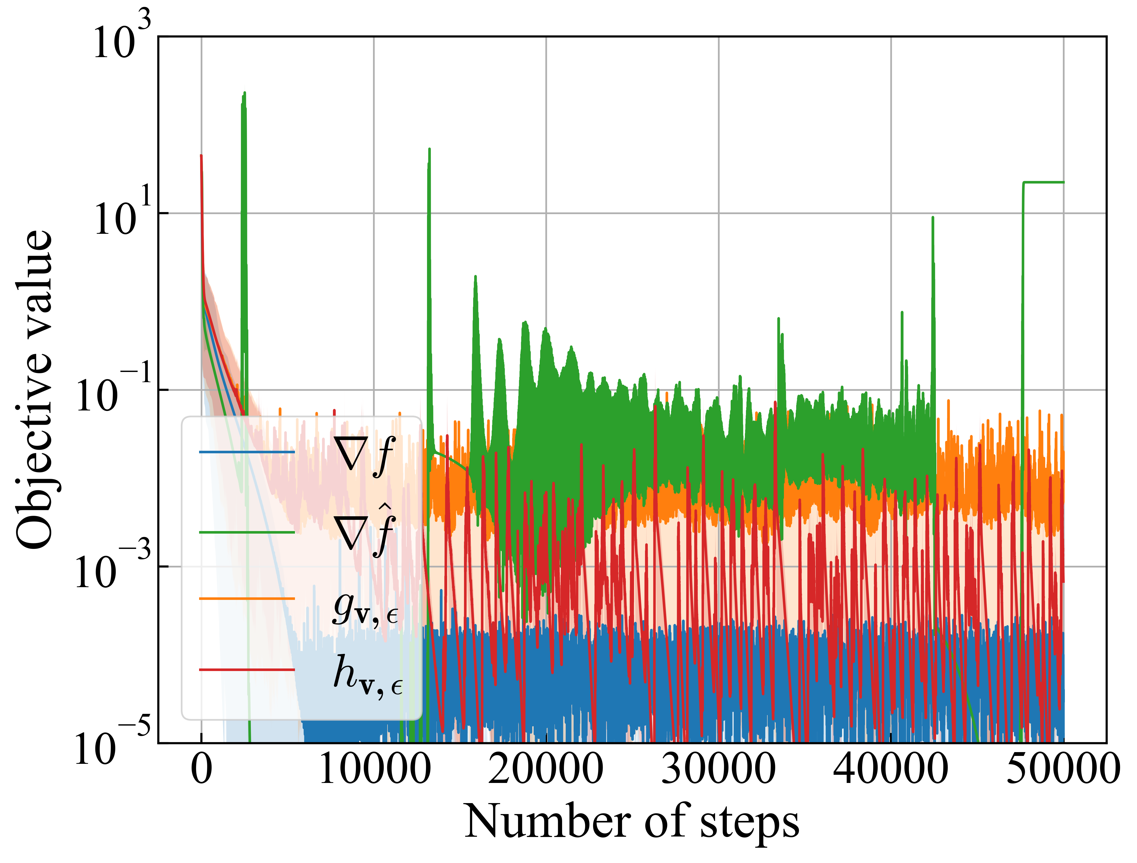
(e) rosenbrock2D

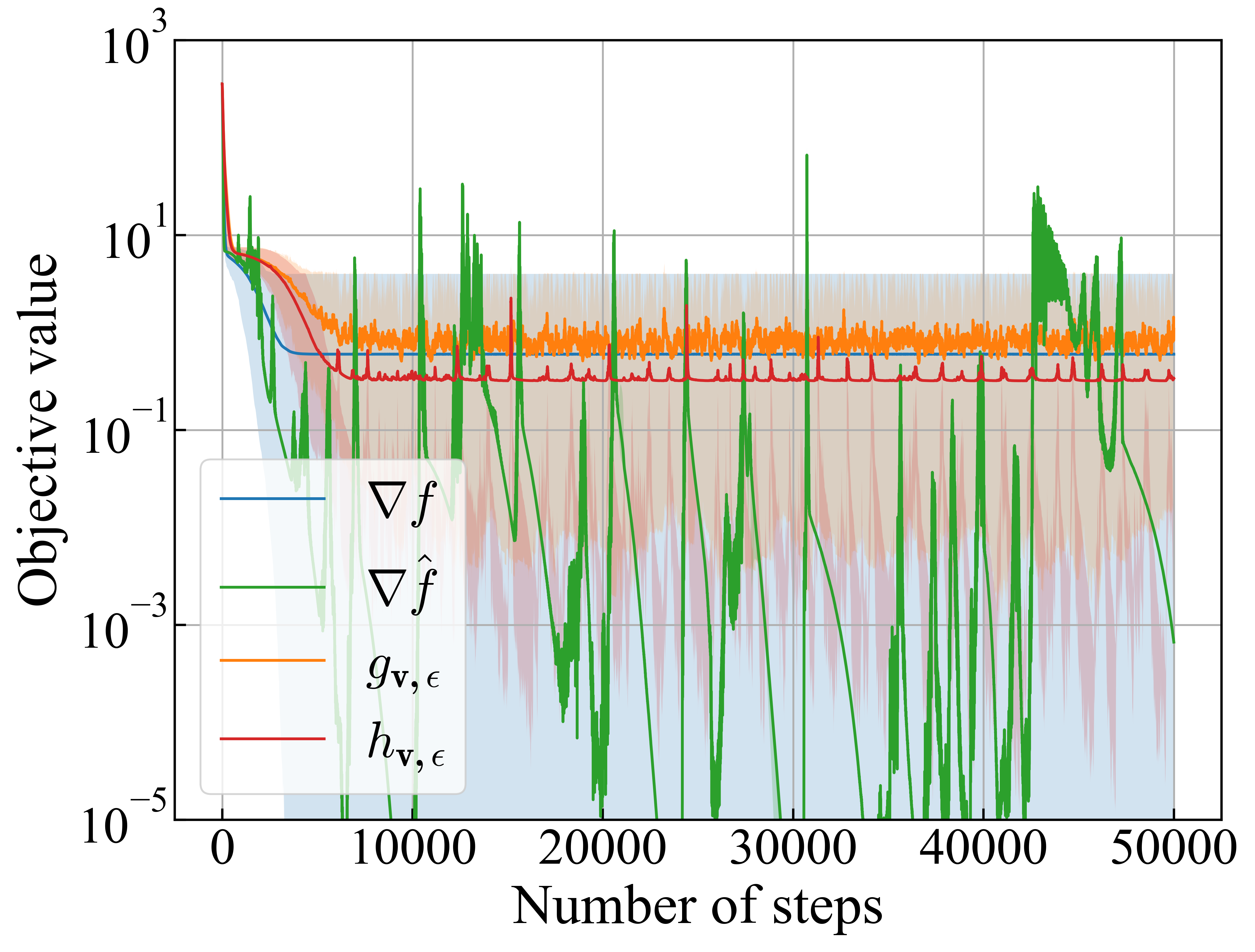
(f) rosenbrock8D

(g) rosenbrock32D

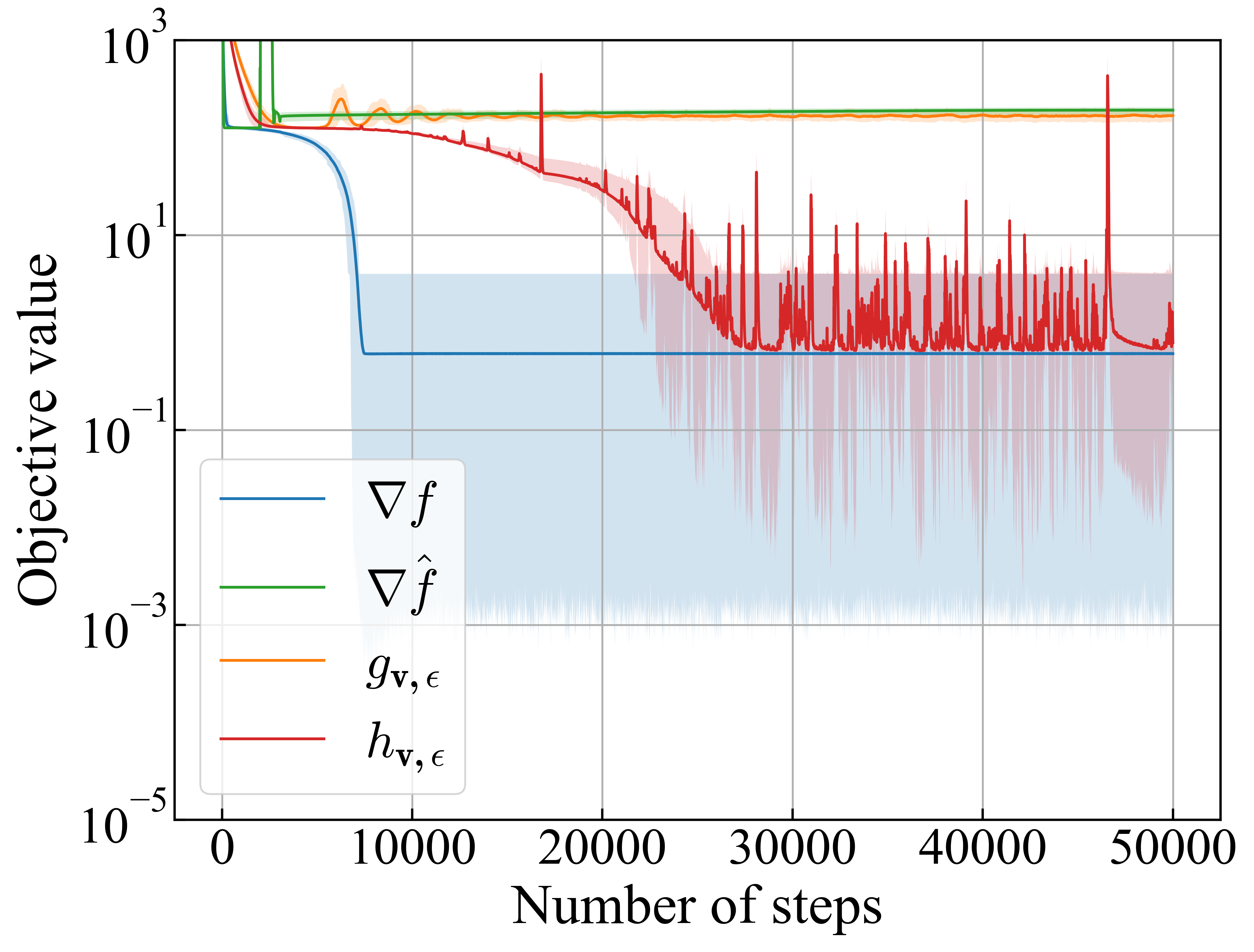
(h) rosenbrock128D

Figure 4: Convergence plots. The horizontal axis is the number of Adam steps, and the vertical axis is the objective value.

Table 4: The standard deviations of objective values obtained using different gradient estimators.

(a) Sphere function

gradient	$d=2$	$d=8$	$d=32$	$d=128$
$\nabla f$	1.61e-12	3.02e-12	5.23e-12	1.04e-11
$\nabla\hat{f}$	2.09e-03	7.38e-06	1.36e-07	1.88e-04
${\bm{g}}_{{\mathbf{v}},\epsilon}$	1.57e-05	2.71e-02	3.44e-01	5.86e+00
${\bm{h}}_{{\mathbf{v}},\epsilon}$ (ours)	9.11e-12	7.28e-11	6.42e-10	1.17e-07

(b) Rosenbrock function

gradient	$d=2$	$d=8$	$d=32$	$d=128$
$\nabla f$	4.49e-05	1.42e+00	1.38e+00	1.43e+00
$\nabla\hat{f}$	1.44e-01	9.66e-07	3.77e-02	6.72e+01
${\bm{g}}_{{\mathbf{v}},\epsilon}$	3.59e-02	3.47e+00	9.85e+00	1.94e+01
${\bm{h}}_{{\mathbf{v}},\epsilon}$ (ours)	9.95e-04	1.08e+00	1.20e+00	1.52e+00

A.4.2 Details of Section 5.1

Task

In both of $P$ and $Q$, solution $u_{\tau}$ has the following form:

$$u_{\tau}(z)=\sum_{i=1}^{N}c_{i}\sin{i\pi z},$$ (85)

where $c_{i}$’s are sampled from different distributions. The task distribution $P$ is a mixture of two distributions $P_{1}$ and $P_{2}$ with weight $p$, i.e. $P=pP_{1}+(1-p)P_{2}$, and $p$ is set to 0.01 in the experiment. In distribution $P_{1}$, we have $c_{i}\sim\mathcal{N}(0,\left|\frac{N+1-2i}{N-1}\right|)$. In distribution $P_{2}$, we have $c_{i}\sim\mathcal{N}(0,1-\left|\frac{N+1-2i}{N-1}\right|)$. Similarly, the task distribution $Q$ is a mixture of two distributions $Q_{1}$ and $Q_{2}$ with weight $q$, i.e. $Q=qQ_{1}+(1-q)Q_{2}$, and $q$ is set to 0.01 in the experiment. In distribution $Q_{1}$, we have $c_{i}\sim\mathcal{N}(0,1-\frac{i}{N})$. In distribution $Q_{2}$, we have $c_{i}\sim\mathcal{N}(0,\frac{i}{N})$. We use $P$ for the Jacobi method and $Q$ for the multigrid method. They are designed to contain a small number of difficult tasks, which make learning difficult (Arisaka & Li, 2023). The discretization size is $N=31$ in the experiments. The number of tasks for training, validation, and test are all $5,000$.

Solver

The solver $f_{\text{MG}}$ is the simplest two-level multigrid solver with the linear prolongation

$$I_{2h}^{h}=\frac{1}{2}\left(\begin{array}[]{ccccc}1&&&&\\ 2&&&&\\ 1&1&&&\\ &2&&&\\ &1&1&&\\ &&2&\ddots&\\ &&1&\ddots&\\ &&&&1\\ &&&2\\ &&&&1\end{array}\right)\in\mathbb{R}^{(N-1)\times(N/2-1)}$$ (86)

and weighted restriction

$$I_{h}^{2h}=\frac{1}{4}\left(\begin{array}[]{lllllllllllll}1&2&1&&&&&&&&\\ &&1&2&1&&&&&&\\ &&&&1&2&1&&&&\\ &&&&&&&\ddots&&&\\ &&&&&&&&&\\ &&&&&&&&1&2&1\end{array}\right)\in\mathbb{R}^{(N/2-1)\times(N-1)}.$$ (87)

In each level, we conduct 4 iterations of the weighted Jacobi method with weight $2/3$ as a smoother.

Meta-solver

The meta-solver $\Psi$ is a fully-connected neural network with one hidden layer with 512 units and SiLU activation function (Elfwing et al., 2018). It takes the right-hand side $b_{\tau}$ as input and gives the coefficients $c_{i}$’s in Equation 85 to construct initial guess $\theta_{\tau}$.

Surrogate model

In Section 5.1, our surrogate model $\hat{f}$ is a fully-connected neural network with three hidden layers with 1024 units and GELU activation function. It takes the initial guess ${\bm{\theta}}_{\tau}$ and the solver’s output $\hat{u}_{\tau}$ as input.

Training

We use the Adam optimizer for all training. For the Jacobi method, we use learning rate $10^{-5}$ for the meta-solver and $5.0\times 10^{-4}$ for the surrogate model. For the multigrid method, we use learning rate $10^{-6}$ for the meta-solver and $5.0\times 10^{-4}$ for the surrogate model. For the supervised baseline, we use learning rate $10^{-4}$. The batch size is set to 256 for all training, and the number of epochs is set to 100. The best model is selected based on the validation loss. The finite difference step size $\epsilon$ is set to $10^{-12}$ for all training. We conducted the experiments with 3 different random seeds.

Results

The standard deviations of the results Table 2 are presented in Table 5.

Table 5: The standard deviations of the results in Table 2.

$\Psi$	gradient	$f=f_{\mathrm{Jac}}$	$f=f_{\mathrm{MG}}$
$\Psi_{\mathrm{SL}}$	-	1.83	0.86
$\Psi_{\mathrm{GBMS}}$	$\nabla f$	0.70	0.45
	$\nabla\hat{f}$	1.35	3.85
	${\bm{g}}_{\mathbf{v}}$	1.70	0.22
	${\bm{g}}_{{\mathbf{v}},\epsilon}$	1.68	0.19
	${\bm{h}}_{\mathbf{v}}$	1.09	0.60
	${\bm{h}}_{{\mathbf{v}},\epsilon}$ (ours)	0.71	0.62

A.4.3 Details of Section 5.2

Task

The problem formulation is based on the demos in the DOLFIN documentation (noa, ). As for the discretization size, we use $3\times 3$ unit square mesh for the biharmonic problem and $3\times 3\times 3$ unit box mesh for the elasticity problem. For the biharmonic problem, the source term $b_{\tau}$ has the following form:

$$b_{\tau}(x,y)=c_{1}\sin(c_{2}\pi x)\sin(c_{3}\pi y),$$ (88)

where

$$c_{1} \sim\mathrm{LogUniform}([10^{-2},10^{2}]),$$ (89)

$$c_{2} \sim\mathrm{DiscreteUniform}([1,2,3,4,5]),$$ (90)

$$c_{3} \sim\mathrm{DiscreteUniform}([1,2,3,4,5]).$$ (91)

The number of tasks for training, validation, and test are all $5,000$ for both problem settings.

Solver

The solver $f_{\text{AMG}}$ is constructed by setting the following PETSc options:

• -ksp_type richardson

• -ksp_initial_guess_nonzero True

• -pc_type gamg

Other options are set to default values.

Meta-solver

The meta-solver $\Psi$ is a fully-connected neural network with one hidden layer with 1024 units and SiLU activation function for both biharmonic and elasticity problem.

Surrogate model

Surrogate model $\hat{f}$ is a fully-connected neural network with three hidden layers with 512 units and GELU activation function for both biharmonic and elasticity problem. It takes the initial guess ${\bm{\theta}}_{\tau}$ and the solver’s solution as input.

Training

We use the Adam optimizer for all training. For the biharmonic problem, we use learning rate $10^{-5}$ for the meta-solver and $5.0\times 10^{-4}$ for the surrogate model. For the elasticity problem, we use learning rate $10^{-4}$ for the meta-solver and $10^{-4}$ for the surrogate model. The batch size is set to 256 for all training. We train them for 1,000 epochs and reduce the learning rate by a factor of 0.1 at 500 and 750 epochs. The best model is selected based on the validation loss.

References

- (1) DOLFIN documentation — DOLFIN documentation. https://fenicsproject.org/olddocs/dolfin/2019.1.0/python/index.html. URL https://fenicsproject.org/olddocs/dolfin/2019.1.0/python/index.html. Accessed: 2024-2-2.
- Ajuria Illarramendi et al. (2020) Ajuria Illarramendi, E., Alguacil, A., Bauerheim, M., Misdariis, A., Cuenot, B., and Benazera, E. Towards an hybrid computational strategy based on Deep Learning for incompressible flows. In AIAA AVIATION 2020 FORUM, AIAA AVIATION Forum. American Institute of Aeronautics and Astronautics, June 2020. doi: 10.2514/6.2020-3058. URL https://doi.org/10.2514/6.2020-3058.
- Alnæs et al. (2015) Alnæs, M., Blechta, J., Hake, J., Johansson, A., Kehlet, B., Logg, A., Richardson, C., Ring, J., Rognes, M. E., and Wells, G. N. The FEniCS Project Version 1.5. Anschnitt, 3(100), December 2015. ISSN 0003-5238. doi: 10.11588/ans.2015.100.20553. URL https://journals.ub.uni-heidelberg.de/index.php/ans/article/view/20553.
- Arisaka & Li (2023) Arisaka, S. and Li, Q. Principled Acceleration of Iterative Numerical Methods Using Machine Learning. In Krause, A., Brunskill, E., Cho, K., Engelhardt, B., Sabato, S., and Scarlett, J. (eds.), Proceedings of the 40th International Conference on Machine Learning, volume 202 of Proceedings of Machine Learning Research, pp. 1041–1059. PMLR, 2023. URL https://proceedings.mlr.press/v202/arisaka23a.html.
- Bacho & Chu (2022) Bacho, F. and Chu, D. Low-Variance Forward Gradients using Direct Feedback Alignment and Momentum. December 2022. URL http://arxiv.org/abs/2212.07282.
- Baker et al. (2019) Baker, N., Alexander, F., Bremer, T., Hagberg, A., Kevrekidis, Y., Najm, H., Parashar, M., Patra, A., Sethian, J., Wild, S., Willcox, K., and Lee, S. Workshop Report on Basic Research Needs for Scientific Machine Learning: Core Technologies for Artificial Intelligence. DOE, February 2019. doi: 10.2172/1478744. URL https://www.osti.gov/servlets/purl/1478744.
- Balay et al. (2023) Balay, S., Abhyankar, S., Adams, M. F., Benson, S., Brown, J., Brune, P., Buschelman, K., Constantinescu, E. M., Dalcin, L., Dener, A., Eijkhout, V., Faibussowitsch, J., Gropp, W. D., Hapla, V., Isaac, T., Jolivet, P., Karpeev, D., Kaushik, D., Knepley, M. G., Kong, F., Kruger, S., May, D. A., McInnes, L. C., Mills, R. T., Mitchell, L., Munson, T., Roman, J. E., Rupp, K., Sanan, P., Sarich, J., Smith, B. F., Zampini, S., Zhang, H., Zhang, H., and Zhang, J. PETSc Web page. https://petsc.org/, 2023. URL https://petsc.org/.
- Baydin et al. (2018) Baydin, A. G., Pearlmutter, B. A., Radul, A. A., and Siskind, J. M. Automatic Differentiation in Machine Learning: a Survey. Journal of machine learning research: JMLR, 18(153):1–43, 2018. ISSN 1532-4435, 1533-7928. URL https://jmlr.org/papers/v18/17-468.html.
- Baydin et al. (2022) Baydin, A. G., Pearlmutter, B. A., Syme, D., Wood, F., and Torr, P. Gradients without Backpropagation. February 2022. URL http://arxiv.org/abs/2202.08587.
- Belouze (2022) Belouze, G. Optimization without Backpropagation. September 2022. URL http://arxiv.org/abs/2209.06302.
- Bottou et al. (2016) Bottou, L., Curtis, F. E., and Nocedal, J. Optimization Methods for Large-Scale Machine Learning. June 2016. URL http://arxiv.org/abs/1606.04838.
- Calì et al. (2023) Calì, S., Hackett, D. C., Lin, Y., Shanahan, P. E., and Xiao, B. Neural-network preconditioners for solving the Dirac equation in lattice gauge theory. Physical Review D, 107(3):034508, February 2023. doi: 10.1103/PhysRevD.107.034508. URL https://link.aps.org/doi/10.1103/PhysRevD.107.034508.
- Chen et al. (2021) Chen, T., Chen, X., Chen, W., Heaton, H., Liu, J., Wang, Z., and Yin, W. Learning to optimize: A primer and A benchmark. March 2021. URL https://jmlr.org/papers/volume23/21-0308/21-0308.pdf.
- Chen et al. (2022) Chen, Y., Dong, B., and Xu, J. Meta-MgNet: Meta multigrid networks for solving parameterized partial differential equations. Journal of computational physics, 455:110996, April 2022. ISSN 0021-9991. doi: 10.1016/j.jcp.2022.110996. URL https://www.sciencedirect.com/science/article/pii/S0021999122000584.
- Cuomo et al. (2022) Cuomo, S., Di Cola, V. S., Giampaolo, F., Rozza, G., Raissi, M., and Piccialli, F. Scientific Machine Learning Through Physics–Informed Neural Networks: Where we are and What’s Next. Journal of scientific computing, 92(3):88, July 2022. ISSN 0885-7474, 1573-7691. doi: 10.1007/s10915-022-01939-z. URL https://doi.org/10.1007/s10915-022-01939-z.
- Elfwing et al. (2018) Elfwing, S., Uchibe, E., and Doya, K. Sigmoid-weighted linear units for neural network function approximation in reinforcement learning. Neural networks: the official journal of the International Neural Network Society, 107:3–11, November 2018. ISSN 0893-6080, 1879-2782. doi: 10.1016/j.neunet.2017.12.012. URL http://dx.doi.org/10.1016/j.neunet.2017.12.012.
- Fournier et al. (2023) Fournier, L., Rivaud, S., Belilovsky, E., Eickenberg, M., and Oyallon, E. Can Forward Gradient Match Backpropagation? June 2023. URL http://arxiv.org/abs/2306.06968.
- Grathwohl et al. (2017) Grathwohl, W., Choi, D., Wu, Y., Roeder, G., and Duvenaud, D. Backpropagation through the Void: Optimizing control variates for black-box gradient estimation. October 2017. URL https://openreview.net/pdf?id=SyzKd1bCW.
- Guo et al. (2022) Guo, Y., Dietrich, F., Bertalan, T., Doncevic, D. T., Dahmen, M., Kevrekidis, I. G., and Li, Q. Personalized Algorithm Generation: A Case Study in Learning ODE Integrators. SIAM Journal of Scientific Computing, 44(4):A1911–A1933, August 2022. ISSN 1064-8275. doi: 10.1137/21M1418629. URL https://doi.org/10.1137/21M1418629.
- Hendrycks & Gimpel (2016) Hendrycks, D. and Gimpel, K. Gaussian Error Linear Units (GELUs). June 2016. URL http://arxiv.org/abs/1606.08415.
- Hsieh et al. (2018) Hsieh, J.-T., Zhao, S., Eismann, S., Mirabella, L., and Ermon, S. Learning Neural PDE Solvers with Convergence Guarantees. In International Conference on Learning Representations, September 2018. URL https://openreview.net/pdf?id=rklaWn0qK7.
- Huang et al. (2020) Huang, J., Wang, H., and Yang, H. Int-Deep: A deep learning initialized iterative method for nonlinear problems. Journal of computational physics, 419:109675, October 2020. ISSN 0021-9991. doi: 10.1016/j.jcp.2020.109675. URL https://www.sciencedirect.com/science/article/pii/S0021999120304496.
- Jacovi et al. (2019) Jacovi, A., Hadash, G., Kermany, E., Carmeli, B., Lavi, O., Kour, G., and Berant, J. Neural network gradient-based learning of black-box function interfaces. January 2019. URL https://openreview.net/pdf?id=r1e13s05YX.
- Jasak (2009) Jasak, H. OpenFOAM: Open source CFD in research and industry. International Journal of Naval Architecture and Ocean Engineering, 1(2):89–94, December 2009. ISSN 2092-6782. doi: 10.2478/IJNAOE-2013-0011. URL https://www.sciencedirect.com/science/article/pii/S2092678216303879.
- Karniadakis et al. (2021) Karniadakis, G. E., Kevrekidis, I. G., Lu, L., Perdikaris, P., Wang, S., and Yang, L. Physics-informed machine learning. Nature Reviews Physics, 3(6):422–440, May 2021. ISSN 2522-5820, 2522-5820. doi: 10.1038/s42254-021-00314-5. URL https://www.nature.com/articles/s42254-021-00314-5.
- Kingma & Ba (2015) Kingma, D. P. and Ba, J. Adam: A Method for Stochastic Optimization. In 3rd International Conference on Learning Representations, 2015. URL http://arxiv.org/abs/1412.6980.
- Luz et al. (2020) Luz, I., Galun, M., Maron, H., Basri, R., and Yavneh, I. Learning Algebraic Multigrid Using Graph Neural Networks. In Iii, H. D. and Singh, A. (eds.), Proceedings of the 37th International Conference on Machine Learning, volume 119 of Proceedings of Machine Learning Research, pp. 6489–6499. PMLR, 2020. URL https://proceedings.mlr.press/v119/luz20a.html.
- (28) Molga, M. and Kwietnia, C. S. . Test functions for optimization needs. https://marksmannet.com/RobertMarks/Classes/ENGR5358/Papers/functions.pdf. URL https://marksmannet.com/RobertMarks/Classes/ENGR5358/Papers/functions.pdf. Accessed: 2023-8-29.
- Nelson (1990) Nelson, B. L. Control Variate Remedies. Operations research, 38(6):974–992, December 1990. ISSN 0030-364X. doi: 10.1287/opre.38.6.974. URL https://doi.org/10.1287/opre.38.6.974.
- Özbay et al. (2021) Özbay, A. G., Hamzehloo, A., Laizet, S., Tzirakis, P., Rizos, G., and Schuller, B. Poisson CNN: Convolutional neural networks for the solution of the Poisson equation on a Cartesian mesh. Data-Centric Engineering, 2, 2021. ISSN 2632-6736. doi: 10.1017/dce.2021.7.
- Polyak (1963) Polyak, B. T. Gradient methods for the minimisation of functionals. USSR Computational Mathematics and Mathematical Physics, 3(4):864–878, January 1963. ISSN 0041-5553. doi: 10.1016/0041-5553(63)90382-3. URL https://www.sciencedirect.com/science/article/pii/0041555363903823.
- Ren et al. (2022) Ren, M., Kornblith, S., Liao, R., and Hinton, G. Scaling forward gradient with local losses. October 2022. URL https://github.com/google-research/.
- Rosenbrock (1960) Rosenbrock, H. H. An Automatic Method for Finding the Greatest or Least Value of a Function. Computer Journal, 3(3):175–184, January 1960. ISSN 0010-4620. doi: 10.1093/comjnl/3.3.175. URL https://academic.oup.com/comjnl/article-pdf/3/3/175/988633/030175.pdf.
- Saad (2003) Saad, Y. Iterative Methods for Sparse Linear Systems: Second Edition. Other Titles in Applied Mathematics. SIAM, April 2003. ISBN 9780898715347. doi: 10.1137/1.9780898718003. URL https://play.google.com/store/books/details?id=qtzmkzzqFmcC.
- Sappl et al. (2019) Sappl, J., Seiler, L., Harders, M., and Rauch, W. Deep Learning of Preconditioners for Conjugate Gradient Solvers in Urban Water Related Problems. June 2019. URL http://arxiv.org/abs/1906.06925.
- Stolarski et al. (2018) Stolarski, T., Nakasone, Y., and Yoshimoto, S. Engineering Analysis with ANSYS Software. Butterworth-Heinemann, January 2018. ISBN 9780081021651. URL https://play.google.com/store/books/details?id=50IyDwAAQBAJ.
- Stüben (2001) Stüben, K. A review of algebraic multigrid. Journal of computational and applied mathematics, 128(1):281–309, March 2001. ISSN 0377-0427. doi: 10.1016/S0377-0427(00)00516-1. URL https://www.sciencedirect.com/science/article/pii/S0377042700005161.
- Takamoto et al. (2022) Takamoto, M., Praditia, T., Leiteritz, R., MacKinlay, D., Alesiani, F., Pflüger, D., and Niepert, M. PDEBENCH: An extensive benchmark for Scientific machine learning. pp. 1596–1611, October 2022. URL https://proceedings.neurips.cc/paper_files/paper/2022/file/0a9747136d411fb83f0cf81820d44afb-Paper-Datasets_and_Benchmarks.pdf.
- Thuerey et al. (2021) Thuerey, N., Holl, P., Mueller, M., Schnell, P., Trost, F., and Um, K. Physics-based Deep Learning. WWW, 2021. URL https://physicsbaseddeeplearning.org.
- Um et al. (2020) Um, K., Brand, R., Fei, Y. r., Holl, P., and Thuerey, N. Solver-in-the-loop: learning from differentiable physics to interact with iterative PDE-solvers. In Proceedings of the 34th International Conference on Neural Information Processing Systems, number Article 513 in NIPS’20, pp. 6111–6122, Red Hook, NY, USA, December 2020. Curran Associates Inc. ISBN 9781713829546. URL https://dl.acm.org/doi/abs/10.5555/3495724.3496237.
- Vaupel et al. (2020) Vaupel, Y., Hamacher, N. C., Caspari, A., Mhamdi, A., Kevrekidis, I. G., and Mitsos, A. Accelerating nonlinear model predictive control through machine learning. Journal of process control, 92:261–270, August 2020. ISSN 0959-1524. doi: 10.1016/j.jprocont.2020.06.012. URL https://www.sciencedirect.com/science/article/pii/S0959152420302481.
- Venkataraman & Amos (2021) Venkataraman, S. and Amos, B. Neural Fixed-Point Acceleration for Convex Optimization. In 8th ICML Workshop on Automated Machine Learning (AutoML), 2021. URL https://openreview.net/forum?id=Vxbpb6XvGgH.
- Vinuesa & Brunton (2021) Vinuesa, R. and Brunton, S. L. The Potential of Machine Learning to Enhance Computational Fluid Dynamics. October 2021. URL http://arxiv.org/abs/2110.02085.
- Willard et al. (2022) Willard, J., Jia, X., Xu, S., Steinbach, M., and Kumar, V. Integrating Scientific Knowledge with Machine Learning for Engineering and Environmental Systems. ACM Comput. Surv., 55(4):1–37, November 2022. ISSN 0360-0300. doi: 10.1145/3514228. URL https://doi.org/10.1145/3514228.
- Williams (1992) Williams, R. J. Simple statistical gradient-following algorithms for connectionist reinforcement learning. Machine learning, 8(3):229–256, May 1992. ISSN 0885-6125. doi: 10.1007/BF00992696. URL https://doi.org/10.1007/BF00992696.