Invertible Residual Rescaling Models

Abstract

Invertible Rescaling Networks (IRNs) and their variants have witnessed remarkable achievements in various image processing tasks like image rescaling. However, we observe that IRNs with deeper networks are difficult to train, thus hindering the representational ability of IRNs. To address this issue, we propose Invertible Residual Rescaling Models (IRRM) for image rescaling by learning a bijection between a high-resolution image and its low-resolution counterpart with a specific distribution. Specifically, we propose IRRM to build a deep network, which contains several Residual Downscaling Modules (RDMs) with long skip connections. Each RDM consists of several Invertible Residual Blocks (IRBs) with short connections. In this way, RDM allows rich low-frequency information to be bypassed by skip connections and forces models to focus on extracting high-frequency information from the image. Extensive experiments show that our IRRM performs significantly better than other state-of-the-art methods with much fewer parameters and complexity. Particularly, our IRRM has respectively PSNR gains of at least 0.3 dB over HCFlow and IRN in the $\times 4$ rescaling while only using 60% parameters and 50% FLOPs. The code will be available at https://github.com/THU-Kingmin/IRRM.

1 Introduction

Image rescaling, which aims to reconstruct high-resolution (HR) images from their corresponding low-resolution (LR) versions by forward sampling, has been widely utilized in large-size data services like storage and transmission. Recently, many flow-based generative methods Ho et al. (2019); Kingma and Dhariwal (2018); Nielsen et al. (2020); Xiao et al. (2020); Liang et al. (2021b) have been applied in image generation and achieved remarkable progress in image rescaling and image super-resolution (SR).

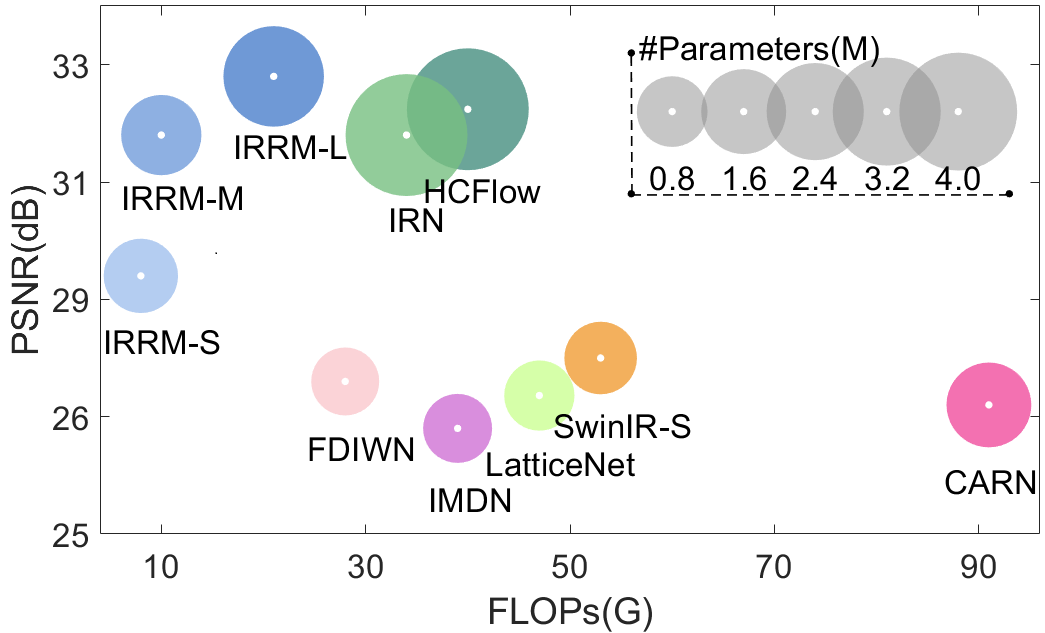
Figure 1: Comparison results of state-of-the-art methods (like IRN and HCFlow) and our IRRM on Urban100 dataset with ×4 rescaling. SR methods combined with bicubic downscaling are also reported. -S, -M, and -L represent the sizes of model parameters respectively, where -S represents small, -M represents medium, and -L represents large. IRRM achieves similar performance using a quarter of parameters and FLOPs of the IRN and HCFlow.

Previous SR methods focus on non-adjustable downscaling kernel (e.g., Bicubic interpolation) rescaling, while omitting their compatibility with the downscaling operation. To remedy this issue, more recent works design adjustable downscaling networks and treat image rescaling as a unified task through an encoder-decoder framework Kim et al. (2018); Li et al. (2018). Specifically, they suggest using an optimal downscaling method as an encoder, trained together with an existing SR module. Despite the improvement of reconstruction quality, these methods still face the problem of the recovery of high-frequency information.

To restore high-frequency details better, Invertible Rescaling Network (IRN) Xiao et al. (2020) has been developed and achieved impressive performance in image rescaling. This type of method focuses on learning the downscaling and upscaling with an invertible neural network, which captures the lost information in a specific distribution and embeds it in the parameters of the model. More recently, HCFlow Liang et al. (2021b) proposes an invertible conditional flow-based model to model the HR-LR relationship, where the high-frequency component is hierarchically conditional on the low-frequency component of the image. Despite the success of IRN in image rescaling, such IRNs are difficult to train, especially with deep layers.

To solve this problem, in this paper, we propose a novel Invertible Residual Rescaling Model (IRRM) to facilitate training while enhancing the representational ability of models. To ease the training, we propose Residual Downscaling Module (RDM) with long skip connections, which serve as the basic block of our IRRM and long skip connection allows rich low-frequency information to be bypassed. In each RDM module, we stack several invertible residual blocks (IRB) to enhance non-linear representation and reduce model degradation with short skip connections. With long and short skip connections, abundant information can be bypassed and thus ease the flow of information. As shown in Fig. 1, our IRRM obtains better results than other state-of-the-art methods with much fewer parameters and complexity.

In summary, the main contributions are as follows:

• We propose a novel Invertible Residual Rescaling Model (IRRM) to build deep networks for highly accurate image rescaling. Our IRRM obtains much better performance than previous methods with much fewer parameters and complexity.

• We propose Residual Downscaling Module (RDM) with long skip connections, equivalent to the second-order wavelet transform, to allow the model to focus on learning the texture information of the image while easing the flow of information.

• Our proposed IRRM introduces the Invertible Residual Block (IRB), which incorporates short skip connections to enhance the model’s nonlinear representational ability. This addition significantly improves the extensibility of the model.

2 Related Work

2.1 Image Super-Resolution

Image super-resolution is a different task from rescaling, aiming to restore HR image given the LR image. However, SR combined with downsampling can be used for image rescaling task. Recently, SR networks have achieved impressive performance based on deep learning Dai et al. (2023); Li et al. (2023); Cui et al. (2023); Zhang et al. (2023); Tang et al. (2024); Guo et al. (2024). SRCNN Dong et al. (2014) is the first work that applies convolutional neural networks for image SR. Later, many methods Kim et al. (2016); Ledig et al. (2017) stack many convolutional layers with residual connections to facilitate the network training. Recently, other advanced methods like RCAN Zhang et al. (2018), SAN Dai et al. (2019) and SwinIR Liang et al. (2021a) build very deep networks to enhance the feature expression ability and have obtained remarkable performance with substantial computational cost. On the other hand, light-weight SR works have been proposed to relieve the problem of computational cost Hui et al. (2019); Luo et al. (2020). For example, the lightweight frequency-aware network (FADN) Xie et al. (2021) is developed to reconstruct different frequency signals with various operations. Instead of designing a lightweight SR network, ClassSR Kong et al. (2021) develops a general framework to accelerate SR networks. However, they seem to have reached the limits of performance for image generation tasks.

2.2 Image Rescaling

The goal of image rescaling is to downscale a high-resolution (HR) image into a visually satisfying low-resolution (LR) image and then restore the HR image from the LR image. Typically, image rescaling concurrently models the enlargement and reduction processes within an encoder-decoder structure to fine-tune the reduction model for subsequent enlargement tasks Kim et al. (2018); Li et al. (2018, 2024a). Recently, IRN Xiao et al. (2020) has been introduced to model the rescaling process using a bijective invertible neural network. During the training phase, IRN effectively captures the high-frequency and low-frequency components. During the testing phase, the HR image can be reconstructed by the generated LR image and a randomly sampled Gaussian distribution. Besides, HCFlow Liang et al. (2021b) assumes that the high-frequency component is dependent on the LR image and employs a hierarchical conditional framework to model the LR image from conditional distribution of the high-frequency component. Nevertheless, these models cannot extend to larger models because of the excessive focus on low frequency information and the lack of residual connections. We address these issues by introducing residual connections and residual enhanced block equivalent to the second-order wavelet transform.

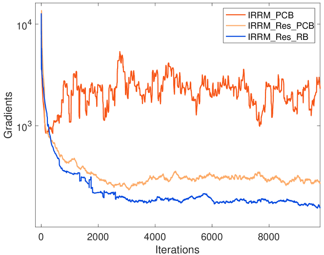
Figure 2: Illustration of training gradients for different models. IRRM with residual connections and enhanced residual block (IRRM_Res_RB) gain a more stable gradient than IRRM w/o residual connections (IRRM_PCB), leading to faster convergence and better performance.

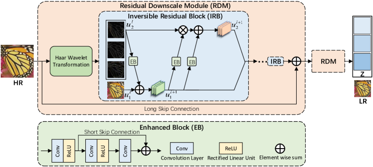
Figure 3: The overall framework of Invertible Residual Rescaling Models (IRRM). IRRM is composed of Residual Downscaling Modules (RDMs), in which Invertible Residual Blocks (IRBs) are stacked after a wavelet transformation. Each IRB contains three Enhanced Blocks (EBs) to enhance the nonlinear representation and mitigate vanishing the gradient problem.

3 Methodology

3.1 Model Specification

Image rescaling involves reconstructing a high-resolution (HR) image $x$ from a low-resolution (LR) image $y$ that is obtained by downscaling $x$. To achieve this, we employ an invertible neural network that models the LR image $y$ and ensures that the distribution of the lost information conforms to a predetermined distribution $z$ (denoted as $[y,z]=f_{\theta}(x)$, where $z$ is sampled from $p(z)$ and $x$ follows the distribution $p(x)$). Conversely, we can reconstruct $x$ through the inverse process using $[y,z]$, denoted as $x=f_{\theta}^{-1}(y,z)$. It is important to note that the lost information $z$ corresponds to the high-frequency details of the image, as per the Nyquist-Shannon sampling theorem Shannon (1949). Instead of explicitly preserving the high-frequency information, we can model $z$ as a Gaussian distribution, thereby obtaining it through sampling from a Gaussian distribution.

3.2 Invertible Residual Rescaling Models

As shown in Fig. 3, our proposed IRRM consists of stacked Residual Downscaling Module (RDM), where RDM further contains one Haar Wavelet Transformation block and several Invertible Residual Blocks (IRBs).

Residual Downscaling Module. RDM utilizes Haar transformation Mallat (1989) to split the input into high and low frequency information. Then IRB learn to model these frequency information into the specified distribution. Specifically, given an HR image $x$ with shape $(H,W,C)$, we first obtain the residual representation of $x$:

$$x_{res}=x-upsample(y)$$ (1)

where $y$ is the LR image and $y=downsample(x)$. Then wavelet transformation decompose $x_{res}$ into global frequency features $[u_{1}^{k},u_{2}^{k}]$:

$$[u_{1}^{k},u_{2}^{k}] =\text{WaveletTransform}(x_{res}^{k})$$ (2)

where $k$ denotes $k^{th}$ layer of the model. $u_{1}$ and $u_{2}$ correspond to high-frequency and low-frequency information, respectively. $x_{res}$ facilitates the model to focus on learning high frequency representations, aiming to recover textures of the image, which is equivalent to the second-order wavelet transform (IRN Xiao et al. (2020) is the first-order wavelet transform). Meanwhile, residual connections make the training process more stable in favour of convergence, as shown in Fig. 2. IRB extracts image features from $u_{1}^{k}$ and $u_{2}^{k}$ to $u_{1}^{k+1}$ and $u_{2}^{k+1}$. After n IRBs’ transformation, we obtain the downscaled image $y$ with shape $(\frac{1}{2}H,\frac{1}{2}W,C)$ and Gaussian distribution $z$ with shape $(\frac{1}{2}H,\frac{1}{2}W,3C)$.

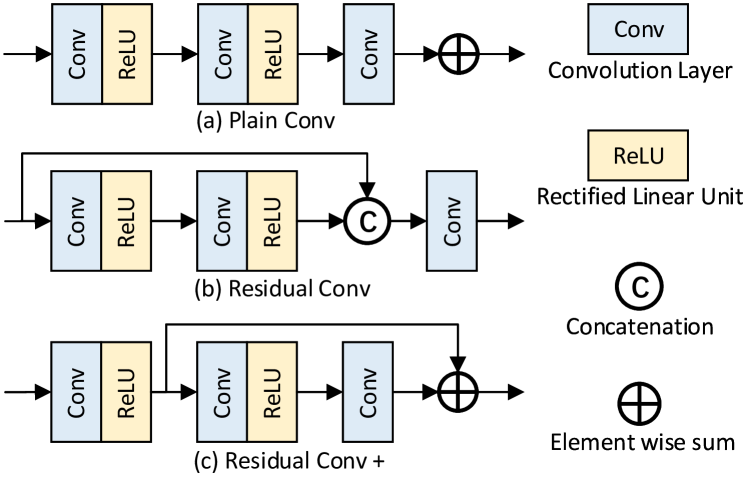
Figure 4: Illustration of Enhanced Blocks (EBs). Three non-linear convolutional blocks in the Invertible Residual Block are compared.

Scale	Models	Paras	Set5	Set10	B100	Urban100	DIV2K
			PSNR / SSIM	PSNR / SSIM	PSNR / SSIM	PSNR / SSIM	PSNR / SSIM
$\times 4$	Bicubic & Bicubic	-	28.42 / 0.8104	26.00 / 0.7027	25.96 / 0.6675	23.14 / 0.6577	26.66 / 0.8521
	Bicubic &SRCNN	$57.3\mathrm{~{}K}$	30.48 / 0.8628	27.50 / 0.7513	26.90 / 0.7101	24.52 / 0.7221	- / -
	Bicubic & CARN	$1.59\mathrm{M}$	32.13 / 0.8937	28.60 / 0.7806	27.58 / 0.7349	26.07 / 0.7837	- / -
	Bicubic & EDSR	$43.1\mathrm{M}$	32.46 / 0.8968	28.80 / 0.7760	27.71 / 0.7420	26.64 / 0.8033	29.38 / 0.9032
	Bicubic & RCAN	$15.6\mathrm{M}$	32.63 / 0.9002	28.87 / 0.7889	27.77 / 0.7436	26.82 / 0.8087	30.77 / 0.8460
	Bicubic & SAN	$15.7\mathrm{M}$	32.64 / 0.9003	28.92 / 0.7888	27.78 / 0.7436	26.79 / 0.8068	- / -
	Bicubic & SwinIR	$11.9\mathrm{M}$	32.92 / 0.9044	29.09 / 0.7950	27.92 / 0.7489	27.45 / 0.8254	- / -
	Bicubic & HAT	$20.8\mathrm{M}$	33.30 / 0.9083	29.47 / 0.8015	28.09 / 0.7551	28.60 / 0.8498	- / -
	TAD & TAU	-	31.81 / -	28.63 / -	28.51 / -	26.63 / -	31.16 / -
	CAR & EDSR	$51.1\mathrm{M}$	33.88 / 0.9174	30.31 / 0.8382	29.15 / 0.8001	29.28 / 0.8711	32.82 / 0.8837
	IRN	$4.35\mathrm{M}$	36.19 / 0.9451	32.67 / 0.9015	31.64 / 0.8826	31.41 / 0.9157	35.07 / 0.9318
	HCFlow	$4.35\mathrm{M}$	36.29 / 0.9468	33.02 / 0.9065	31.74 / 0.8864	31.62 / 0.9206	35.23 / 0.9346
	IRRM-S (ours)	$991\mathrm{~{}K}$	33.20 / 0.8927	29.75 / 0.8441	30.82 / 0.8547	30.21 / 0.8825	33.45 / 0.8901
	IRRM-M (ours)	$1.32\mathrm{M}$	36.30 / 0.9491	32.84 / 0.9098	31.93 / 0.8938	31.36 / 0.9193	35.31 / 0.9373
	IRRM-L (ours)	$2.64\mathrm{M}$	36.85 / 0.9541	33.37 / 0.9174	32.30 / 0.9016	31.94 / 0.9278	35.78 / 0.9429
$\times 2$	Bicubic & Bicubic	-	33.66 / 0.9299	30.24 / 0.8688	29.56 / 0.8431	26.88 / 0.8403	31.01 / 0.9393
	Bicubic & SRCNN	$57.3\mathrm{~{}K}$	36.66 / 0.9542	32.45 / 0.9067	31.36 / 0.8879	29.50 / 0.8946	- / -
	Bicubic & CARN	$1.59\mathrm{M}$	37.76 / 0.9590	33.52 / 0.9166	32.09 / 0.8978	31.92 / 0.9256	- / -
	Bicubic & EDSR	$40.7\mathrm{M}$	38.20 / 0.9606	34.02 / 0.9204	32.37 / 0.9018	33.10 / 0.9363	35.12 / 0.9699
	Bicubic & RCAN	$15.4\mathrm{M}$	38.27 / 0.9614	34.12 / 0.9216	32.41 / 0.9027	33.34 / 0.9384	- / -
	Bicubic & SAN	$15.7\mathrm{M}$	38.31 / 0.9620	34.07 / 0.9213	32.42 / 0.9208	33.10 / 0.9370	- / -
	Bicubic & SwinIR	$11.8\mathrm{M}$	38.42 / 0.9623	34.46 / 0.9250	32.53 / 0.9041	33.81 / 0.9427	- / -
	Bicubic & HAT	$20.9\mathrm{M}$	38.91 / 0.9646	35.29 / 0.9293	32.74 / 0.9066	35.09 / 0.9505	- / -
	TAD & TAU	-	38.46 / -	35.52 / -	36.68 / -	35.03 / -	39.01 / -
	CAR & EDSR	$52.8\mathrm{M}$	38.94 / 0.9658	35.61 / 0.9404	33.83 / 0.9262	35.24 / 0.9572	38.26 / 0.9599
	IRN	$1.66\mathrm{M}$	43.99 / 0.9871	40.79 / 0.9778	41.32 / 0.9876	39.92 / 0.9865	44.32 / 0.9908
	IRRM-S (ours)	$1.06\mathrm{M}$	44.30 / 0.9895	40.95 / 0.9821	40.55 / 0.9859	40.05 / 0.9885	43.98 / 0.9907
	IRRM-M (ours)	$1.59\mathrm{M}$	44.85 / 0.9904	41.39 / 0.9837	40.95 / 0.9872	40.50 / 0.9896	44.44 / 0.9917
	IRRM-L (ours)	$2.12\mathrm{M}$	46.41 / 0.9921	42.51 / 0.9860	43.28 / 0.9924	41.82 / 0.9922	46.35 / 0.9945

Table 1: Quantitative comparison results (PSNR / SSIM) of different rescaling methods on datasets: Set5, Set14, BSD100, Urban100, and DIV2K. -S, -M, and -L are used to denote small, medium, and large parameters of the model, respectively. Best and second best results are in red and blue colors. We report the mean results of 5 draws for IRN, HCFlow and our IRRM. Differences of PSNR and SSIM from different z samples are less than 0.03 and 0.005, respectively.

Invertible Residual Block. To be specific, wavelet features $u_{1}^{k}$ and $u_{2}^{k}$ are fed into stacked IRBs to the obtains LR $y$ and latent variable $z$. We adopt the general coupling layer for invertible architecture Jacobsen et al. (2018); Behrmann et al. (2019). The output of each IRB can be defined as:

$$u_{1}^{k+1} =u_{1}^{k}\cdot(\text{EB}(u_{2}^{k}))+\text{EB}(u_{2}^{k})$$ (3)

$$u_{2}^{k+1} =u_{2}^{k}\cdot(\text{EB}(u_{1}^{k+1}))+\text{EB}(u_{1}^{k+1})$$

$$u_{2}^{k} =(u_{2}^{k+1}-\text{EB}(u_{1}^{k+1}))/(\text{EB}(u_{1}^{k+1}))$$

$$u_{1}^{k} =(u_{1}^{k+1}-\text{EB}(u_{2}^{k}))/(\text{EB}(u_{2}^{k}))$$

where $u_{1}^{k+1}$ and $u_{2}^{k+1}$ are the output of current IRB and the input of next IRB. Note that EB can be arbitrary convolutional unit to enhance the non-linear capability of the model. In our IRRM, we employ two residual connected convolutional blocks and one plain convolutional block He et al. (2016); Liu et al. (2021) as the enhanced block, as shown in Fig. 4. RB in EB enhances the non-linearity and the residual connections make the model training stable, solving the problem of unstable training of plain convolutional layers.

3.3 Loss Functions

Image rescaling aims to reconstruct exactly the HR image while generating visually pleasing LR image. Following IRN Xiao et al. (2020), our IRRM is trained by minimizing the following loss:

$$\mathcal{L}= \lambda_{1}\mathcal{L}_{back}(x,x_{back})+\lambda_{2}\mathcal{L}_{forw}(y,y_{forw})$$ (4)

$$+\lambda_{3}\mathcal{L}_{latent}(z)$$

where $x$ is ground-truth HR image, $y$ is ground-truth LR image, and $x_{back}$ is reconstructed HR image from forward LR image $y_{forw}$ and sampling latent variable $z$.

$\mathcal{L}_{back}$ is the $l_{1}$ pixel loss defined as:

$$\mathcal{L}_{back}(x_{back},x)=\frac{1}{M}\sum_{i=1}^{M}\|f_{\theta}^{-1}(y,z)-x\|_{1}$$ (5)

where $M$ is the number of pixels and $x_{back}=f_{\theta}^{-1}(y,z)$.

Likewise, $\mathcal{L}_{forw}$ is the $l_{2}$ pixel loss defined as:

$$\mathcal{L}_{forw}(y_{forw},y)=\frac{1}{N}\sum_{i=1}^{N}\|f_{\theta}^{y}(x)-y\|_{2}$$ (6)

where $N$ is the number of pixels and $y_{forw}=f_{\theta}^{y}(x)$ is the ground-truth LR image.

The last term $\mathcal{L}_{latent}(z)$ is the $l_{2}$ regularization on the latent variable $z$ to ensure that $z$ follows a Gaussian distribution. We jointly optimise the invertible architecture $f$ by utilizing both forward and backward losses.

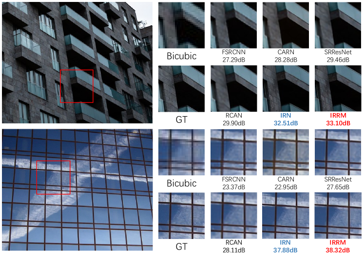
Figure 5: Visual results of upscaling the $4\times$ downscaled images. The right images are $128\times 128$ which is a patch of the left images. IRRM recovers rich textures and realistic details, leading to better recovery performance. IRRM achieves better performance with an increased PSNR of 4 dB over RCAN and 0.6 dB over IRN

4 Experiments

4.1 Settings

Datasets. The DIV2K dataset Agustsson and Timofte (2017) is adopted to train our IRRM. Firstly, we prepare the HR images by cropping the original images with steps 240 to $480\times 480$. These HR images are down-sampled with scaling factors 0.25 and 0.5 to obtain the LR images. Besides, we evaluate our models with PSNR and SSIM metrics (Y channel) on commonly used benchmarks: Set5 Bevilacqua et al. (2012), Set14 Yang et al. (2010), B100 Martin et al. (2001), Urban100 Huang et al. (2015) and DIV2K valid Agustsson and Timofte (2017) datasets. For a fair comparison with baselines, all images are with size $1280\times 720$ to calculate FLOPs and we take the mean within a test set.

Training Details. Our IRRM is composed of one or two Residual Downscaling Modules (RDMs), containing eight Invertible Residual Blocks (IRBs). These models are trained using the ADAM Kingma and Ba (2014) optimizer with $\beta_{1}=0.9$ and $\beta_{2}=0.999$. The batch size is set to 16 for per GPU, and the initial learning rate is fixed at $2\times 10^{-4}$, which decays by half every 10k iterations. PyTorch is used as the implementation framework. $\lambda_{1}$, $\lambda_{2}$ and $\lambda_{3}$ are set to 8, 8 and 1, respectively. Finally, we augment training images by flipping and rotating.

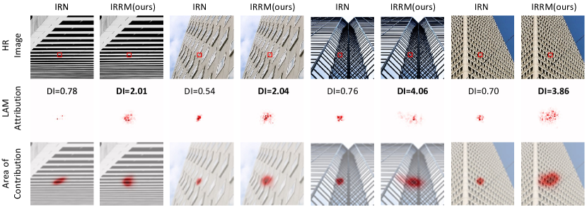
Figure 6: Visual results of Local Attribution Maps (LAM) for IRN and IRRM (ours). The LAM, calculated by diffusion index (DI), indicates the contribution of each pixel in the input image w.r.t. the patch marked with a red box in the HR image. A higher DI, illustrated in the second line, means a wider area of attention in the third lines.

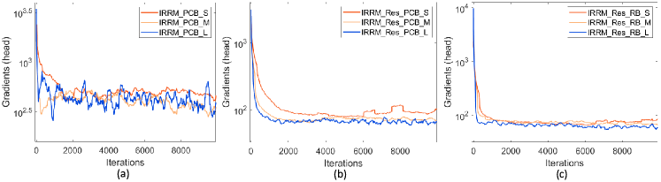
Figure 7: Exploring model extensibility. As the model gets larger, IRRM without residual connections is extremely unstable in training. IRRM with residual connections and RB is stable and converges easily. PCB : plain convolution block. Res : residual connections in the Residual Downscaling Module. RB : residual block in the Invertible Residual Block. -S, -M, -L : denoted the model sizes.

4.2 Comparison with State-of-the-art Method

Performance Comparison. We compare our IRRM with State-of-the-arts (like HAT Chen et al. (2023), IRN Xiao et al. (2020), HCFlow Liang et al. (2021b) and so on) on commonly used datasets (Set5 Bevilacqua et al. (2012), Set14 Yang et al. (2010), B100 Martin et al. (2001), Urban100 Huang et al. (2015) and DIV2K valid Agustsson and Timofte (2017)) evaluated by Peak Signal-to-Noise Ratio (PSNR) and Structural Similarity Index Measure (SSIM).

As shown in Table 1, the quantitative results of different rescaling methods are summarized. IRRM significantly outperforms previous state-of-the-art methods regarding PSNR and SSIM in five benchmark datasets. Previous SR methods have limited performance in rescaling tasks because of fixed downscaling process. IRN Xiao et al. (2020), HCFlow Liang et al. (2021b) and our IRRM optimize the upscaling and downscaling models by joint optimization based on the invertible architecture, further boosting the the PSNR metric about 5 dB on different benchmark datasets. Specifically, HCFlow achieves better performance with an increased PSNR of 0.2 dB over IRN in the $\times 4$ rescaling. Further, compared with IRN, our proposed IRRM improves 0.6 dB PSNR in the $\times 4$ rescaling and 2 dB PSNR in the $\times 2$ rescaling while only using half of the parameters. IRRM-M achieves performance comparable to IRN with only 1/4 parameters, and IRRM-S achieves performance well beyond that of previous SR methods with less than 1M parameters. These experimental results demonstrate that our model is efficient.

Besides, we visualize the rescaling resulting images as shown in Fig. 5, including two common scenes. HR images restored by IRRM achieve better visual quality and rich textures than those of previous state-of-the-art methods. This advanced capability is attributed to residual connections in RDM, which enables the model to concentrate on learning high-frequency information, and the incorporation of Invertible Residual Block (IRB), which strengthens non-linear capacity of the model.

Interpretation with Local Attribution Maps (LAM). We analyze the diffusion index (DI) of previous methods and IRRM to better understand why IRRM works. DI is applied to measure local attribution maps (LAM Gu and Dong (2021)) from the input image to output image of models. When considering the same local patch, if LAM contains a greater range of pixels or encompasses a larger area, it can be inferred that the models have effectively utilized information from a larger number of pixels. As shown in Fig. 6, our IRRM utilizes a wider range of pixels for better rescaling for models. Specifically, the DI of IRRM is four times that of IRN due to the fact that we have introduced residual connections in IRRM, which makes the receptive field of the model larger.

RDM	IRB	Set5	Set10	B100	Urban100
✗	PCB	35.23	31.55	30.77	29.63
✗	RB	36.56	31.90	31.03	30.25
✔	PCB	36.80	33.27	32.22	31.68
✔	RB	36.85	33.37	32.30	31.94
✔	RB+	36.46	32.81	31.76	31.23
✗	4 RBs	35.07	31.41	30.57	29.51
✔	4 RBs	36.30	32.84	31.93	31.36
✗	8 RBs	35.56	31.90	31.03	30.25
✔	8 RBs	36.85	33.37	32.30	31.94
✗	12 RBs	35.48	31.90	30.87	29.93
✔	12 RBs	36.89	33.41	32.32	31.94

Table 2: Ablation study of the effect of proposed Residual Downscaling Module (RDM) and Invertible Residual Block (IRB). The first column indicates whether residual connections are used in the RDM. The second column indicates the convolutional blocks in the IRB. N RBs denotes the IRB uses n RBs.

4.3 Ablation Study

In the ablation study, we replace the modules proposed in the IRRM to evaluate the effect of RDM and IRB. Model extensibility and effects of loss functions are also evaluated.

Residual Downscaling Module. We discard residual connections of RDM to investigate the contribution of them. As shown in Fig. 7, IRRM is more extensible with residual connections and RB. As the model gets deeper, the absence of residual connections can lead to instability of the model gradient, with problems of gradient vanishing and gradient explosion. Furthermore, IRRM with residual connections has better extensibility while the performance degrades as the network gets larger (8 RBs $\rightarrow$ 12 RBs) without residual connections, as shown below in Table 2.

Invertible Residual Block. To investigate the effects of Residual Block (EB) in the IRB, we replace it with a plain convolutional layer. The detailed structure is shown in Fig. 4. As shown above in Table 2, RB performs better than PCB, due to residual connections. In addition, RB+ achieves comparable performance through half of the parameters.

As illustrated in Table 3, the performance of IRRM with residual connections and RB improves as the model size increases (IRRM-S (RB, Res) $\rightarrow$ IRRM-M (RB, Res) $\rightarrow$ IRRM-L (RB, Res)). However, in the case of IRRM without residual connections, the performance does not improve as the model size increases (IRRM-S (PCB) $\rightarrow$ IRRM-M (PCB) $\rightarrow$ IRRM-L (PCB)). Notably, IRRM-M (PCB) achieves superior performance in this scenario. This shows the excellent extensibility of our proposed IRRM.

Models	Set5	Set10	B100	Urban100
IRRM-S (PCB)	34.86	31.21	30.43	29.09
IRRM-M (PCB)	35.23	31.55	30.77	29.63
IRRM-L (PCB)	34.68	31.53	30.73	29.66
IRRM-S (PCB, Res)	36.09	32.42	31.68	31.14
IRRM-M (PCB, Res)	36.80	33.27	32.22	31.68
IRRM-L (PCB, Res)	36.72	33.29	32.19	31.71
IRRM-S (RB, Res)	36.30	32.87	31.88	31.30
IRRM-M (RB, Res)	36.85	33.37	32.30	31.94
IRRM-L (RB, Res)	36.89	33.41	32.32	31.94

Table 3: Exploring different model extensibility. IRRM (PCB): IRRM with Plain convolutional block. IRRM (PCB, Res): IRRM with plain convolutional blocks and residual connections. IRRM (RB, Res): IRRM with residual blocks and residual connections.

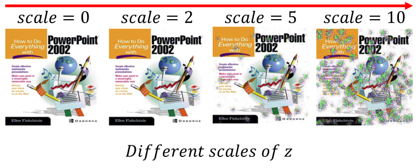
Figure 8: Visual results of employing IRRM to HR images using different scales of $z$ samples. A Gaussian distribution is used in training $z$, and scaled samples drawn from this distribution are used to illustrate upscaling results.

4.4 Visualisation on the Influence of $z$

We also analyse the effect of different scales of z on the reconstructed HR image, as shown in Fig. 8. It is observed that our proposed IRRM is insensitive to the Gaussian distribution z and generates unrealistic high-frequency details only when z is very large. $z$ represents the high-frequency components in an image and is typically sparse. However, changes in $z$ have a significant impact on the image details. Therefore, it is essential for the model to exhibit a high tolerance towards $z$ in order to preserve image details effectively.

4.5 Real-world Datasets

Real-world dataset is also applicable for our method, since the inputs of our model are high-resolution images, whether they are real-world datasets or synthetic datasets. The results are shown in Table 4.

Method	RealSR-cano		RealSR-Nikon
	PSNR $\uparrow$	LPIPS $\downarrow$	PSNR $\uparrow$	LPIPS $\downarrow$
ESRGAN	27.67	0.412	27.46	0.425
SwinIR	26.64	0.357	25.76	0.364
HAT	26.68	0.342	25.85	0.358
Ours	29.12	0.327	28.87	0.336

Table 4: Comparison results with existing state-of-the-art SR methods on real-world datasets.

With the recent rapid development in multimodality Bai et al. (2024); Li et al. (2024b); Gao et al. (2023); Wang et al. (2023), we will also explore the help of textual cues in the future to better exploit the potential of the Rescaling task.

5 Conclusion

In this paper, we develop an efficient and light-weight framework IRRM for image rescaling. IRRM learns a bijection between HR image and LR image as well as specific distribution $z$ so that it is information lossless and invertible. Specifically, IRRM introduces residual connections in the RDM, equivalent to a second-order wavelet transform. Direct modeling of high frequency information reduces the training difficulty and allows the training gradient to trend towards brown noise rather than white noise. Besides, we propose IRB to enhance non-linear representation and reduce model degradation, while the block is lightweight and lossless. This addition significantly improves the extensibility of the model.

6 Acknowledgements

This work is supported in part by the National Natural Science Foundation of China, under Grant (62302309, 62171248), Shenzhen Science and Technology Program (JCYJ20220818101014030, JCYJ20220818101012025), and the PCNL KEY project (PCL2023AS6-1), and Tencent “Rhinoceros Birds” - Scientific Research Foundation for Young Teachers of Shenzhen University.

References

- Agustsson and Timofte [2017] Eirikur Agustsson and Radu Timofte. Ntire 2017 challenge on single image super-resolution: Dataset and study. In Proceedings of the IEEE conference on computer vision and pattern recognition workshops, pages 126–135, 2017.
- Bai et al. [2024] Jiawang Bai, Kuofeng Gao, Shaobo Min, Shu-Tao Xia, Zhifeng Li, and Wei Liu. Badclip: Trigger-aware prompt learning for backdoor attacks on clip. In CVPR, 2024.
- Behrmann et al. [2019] Jens Behrmann, Will Grathwohl, Ricky TQ Chen, David Duvenaud, and Jörn-Henrik Jacobsen. Invertible residual networks. In International Conference on Machine Learning, pages 573–582. PMLR, 2019.
- Bevilacqua et al. [2012] Marco Bevilacqua, Aline Roumy, Christine Guillemot, and Marie line Alberi Morel. Low-complexity single-image super-resolution based on nonnegative neighbor embedding. In Proceedings of the British Machine Vision Conference, pages 135.1–135.10. BMVA Press, 2012.
- Chen et al. [2023] Xiangyu Chen, Xintao Wang, Jiantao Zhou, Yu Qiao, and Chao Dong. Activating more pixels in image super-resolution transformer. In Proceedings of the IEEE/CVF Conference on Computer Vision and Pattern Recognition, pages 22367–22377, 2023.
- Cui et al. [2023] Yuning Cui, Wenqi Ren, Xiaochun Cao, and Alois Knoll. Image restoration via frequency selection. IEEE Transactions on Pattern Analysis and Machine Intelligence, 2023.
- Dai et al. [2019] Tao Dai, Jianrui Cai, Yongbing Zhang, Shu-Tao Xia, and Lei Zhang. Second-order attention network for single image super-resolution. In Proceedings of the IEEE/CVF conference on computer vision and pattern recognition, pages 11065–11074, 2019.
- Dai et al. [2023] Tao Dai, Mengxi Ya, Jinmin Li, Xinyi Zhang, Shu-Tao Xia, and Zexuan Zhu. Cfgn: A lightweight context feature guided network for image super-resolution. IEEE Transactions on Emerging Topics in Computational Intelligence, 2023.
- Dong et al. [2014] Chao Dong, Chen Change Loy, Kaiming He, and Xiaoou Tang. Learning a deep convolutional network for image super-resolution. In European conference on computer vision, pages 184–199. Springer, 2014.
- Gao et al. [2023] Kuofeng Gao, Yang Bai, Jindong Gu, Yong Yang, and Shu-Tao Xia. Backdoor defense via adaptively splitting poisoned dataset. In CVPR, 2023.
- Gu and Dong [2021] Jinjin Gu and Chao Dong. Interpreting super-resolution networks with local attribution maps. In Proceedings of the IEEE/CVF Conference on Computer Vision and Pattern Recognition, pages 9199–9208, 2021.
- Guo et al. [2024] Hang Guo, Jinmin Li, Tao Dai, Zhihao Ouyang, Xudong Ren, and Shu-Tao Xia. Mambair: A simple baseline for image restoration with state-space model. arXiv preprint arXiv:2402.15648, 2024.
- He et al. [2016] Kaiming He, Xiangyu Zhang, Shaoqing Ren, and Jian Sun. Deep residual learning for image recognition. In Proceedings of the IEEE conference on computer vision and pattern recognition, pages 770–778, 2016.
- Ho et al. [2019] Jonathan Ho, Xi Chen, Aravind Srinivas, Yan Duan, and Pieter Abbeel. Flow++: Improving flow-based generative models with variational dequantization and architecture design. In International Conference on Machine Learning, pages 2722–2730. PMLR, 2019.
- Huang et al. [2015] Jia-Bin Huang, Abhishek Singh, and Narendra Ahuja. Single image super-resolution from transformed self-exemplars. In Proceedings of the IEEE conference on computer vision and pattern recognition, pages 5197–5206, 2015.
- Hui et al. [2019] Zheng Hui, Xinbo Gao, Yunchu Yang, and Xiumei Wang. Lightweight image super-resolution with information multi-distillation network. In Proceedings of the 27th acm international conference on multimedia, pages 2024–2032, 2019.
- Jacobsen et al. [2018] Jörn-Henrik Jacobsen, Arnold Smeulders, and Edouard Oyallon. i-revnet: Deep invertible networks. arXiv preprint arXiv:1802.07088, 2018.
- Kim et al. [2016] Jiwon Kim, Jung Kwon Lee, and Kyoung Mu Lee. Accurate image super-resolution using very deep convolutional networks. In Proceedings of the IEEE conference on computer vision and pattern recognition, pages 1646–1654, 2016.
- Kim et al. [2018] Heewon Kim, Myungsub Choi, Bee Lim, and Kyoung Mu Lee. Task-aware image downscaling. In Proceedings of the European conference on computer vision (ECCV), pages 399–414, 2018.
- Kingma and Ba [2014] Diederik P Kingma and Jimmy Ba. Adam: A method for stochastic optimization. arXiv preprint arXiv:1412.6980, 2014.
- Kingma and Dhariwal [2018] Durk P Kingma and Prafulla Dhariwal. Glow: Generative flow with invertible 1x1 convolutions. Advances in neural information processing systems, 31, 2018.
- Kong et al. [2021] Xiangtao Kong, Hengyuan Zhao, Yu Qiao, and Chao Dong. Classsr: A general framework to accelerate super-resolution networks by data characteristic. In Proceedings of the IEEE/CVF Conference on Computer Vision and Pattern Recognition, pages 12016–12025, 2021.
- Ledig et al. [2017] Christian Ledig, Lucas Theis, Ferenc Huszár, Jose Caballero, Andrew Cunningham, Alejandro Acosta, Andrew Aitken, Alykhan Tejani, Johannes Totz, Zehan Wang, et al. Photo-realistic single image super-resolution using a generative adversarial network. In Proceedings of the IEEE conference on computer vision and pattern recognition, pages 4681–4690, 2017.
- Li et al. [2018] Yue Li, Dong Liu, Houqiang Li, Li Li, Zhu Li, and Feng Wu. Learning a convolutional neural network for image compact-resolution. IEEE Transactions on Image Processing, 28(3):1092–1107, 2018.
- Li et al. [2023] Jinmin Li, Tao Dai, Mingyan Zhu, Bin Chen, Zhi Wang, and Shu-Tao Xia. Fsr: A general frequency-oriented framework to accelerate image super-resolution networks. In Proceedings of the AAAI Conference on Artificial Intelligence, volume 37, pages 1343–1350, 2023.
- Li et al. [2024a] Jinmin Li, Tao Dai, Jingyun Zhang, Kang Liu, Jun Wang, Shaoming Wang, Shu-Tao Xia, et al. Boundary-aware decoupled flow networks for realistic extreme rescaling. arXiv preprint arXiv:2405.02941, 2024.
- Li et al. [2024b] Jinmin Li, Kuofeng Gao, Yang Bai, Jingyun Zhang, Shu-tao Xia, and Yisen Wang. Fmm-attack: A flow-based multi-modal adversarial attack on video-based llms. arXiv preprint arXiv:2403.13507, 2024.
- Liang et al. [2021a] Jingyun Liang, Jiezhang Cao, Guolei Sun, Kai Zhang, Luc Van Gool, and Radu Timofte. Swinir: Image restoration using swin transformer. In Proceedings of the IEEE/CVF International Conference on Computer Vision, pages 1833–1844, 2021.
- Liang et al. [2021b] Jingyun Liang, Andreas Lugmayr, Kai Zhang, Martin Danelljan, Luc Van Gool, and Radu Timofte. Hierarchical conditional flow: A unified framework for image super-resolution and image rescaling. In Proceedings of the IEEE/CVF International Conference on Computer Vision (ICCV), pages 4076–4085, October 2021.
- Liu et al. [2021] Yang Liu, Zhenyue Qin, Saeed Anwar, Pan Ji, Dongwoo Kim, Sabrina Caldwell, and Tom Gedeon. Invertible denoising network: A light solution for real noise removal. In Proceedings of the IEEE/CVF conference on computer vision and pattern recognition, pages 13365–13374, 2021.
- Luo et al. [2020] Xiaotong Luo, Yuan Xie, Yulun Zhang, Yanyun Qu, Cuihua Li, and Yun Fu. Latticenet: Towards lightweight image super-resolution with lattice block. In European Conference on Computer Vision, pages 272–289. Springer, 2020.
- Mallat [1989] Stephane G Mallat. A theory for multiresolution signal decomposition: the wavelet representation. IEEE transactions on pattern analysis and machine intelligence, 11(7):674–693, 1989.
- Martin et al. [2001] David Martin, Charless Fowlkes, Doron Tal, and Jitendra Malik. A database of human segmented natural images and its application to evaluating segmentation algorithms and measuring ecological statistics. In Proceedings Eighth IEEE International Conference on Computer Vision. ICCV 2001, volume 2, pages 416–423. IEEE, 2001.
- Nielsen et al. [2020] Didrik Nielsen, Priyank Jaini, Emiel Hoogeboom, Ole Winther, and Max Welling. Survae flows: Surjections to bridge the gap between vaes and flows. Advances in Neural Information Processing Systems, 33:12685–12696, 2020.
- Shannon [1949] Claude E Shannon. Communication in the presence of noise. Proceedings of the IRE, 37(1):10–21, 1949.
- Tang et al. [2024] Xiaolong Tang, Meina Kan, Shiguang Shan, Zhilong Ji, Jinfeng Bai, and Xilin Chen. Hpnet: Dynamic trajectory forecasting with historical prediction attention. arXiv preprint arXiv:2404.06351, 2024.
- Wang et al. [2023] Yuting Wang, Jinpeng Wang, Bin Chen, Ziyun Zeng, and Shu-Tao Xia. Contrastive masked autoencoders for self-supervised video hashing. In Proceedings of the AAAI Conference on Artificial Intelligence, volume 37, pages 2733–2741, 2023.
- Xiao et al. [2020] Mingqing Xiao, Shuxin Zheng, Chang Liu, Yaolong Wang, Di He, Guolin Ke, Jiang Bian, Zhouchen Lin, and Tie-Yan Liu. Invertible image rescaling. In Computer Vision–ECCV 2020: 16th European Conference, Glasgow, UK, August 23–28, 2020, Proceedings, Part I 16, pages 126–144. Springer, 2020.
- Xie et al. [2021] Wenbin Xie, Dehua Song, Chang Xu, Chunjing Xu, Hui Zhang, and Yunhe Wang. Learning frequency-aware dynamic network for efficient super-resolution. In Proceedings of the IEEE/CVF International Conference on Computer Vision, pages 4308–4317, 2021.
- Yang et al. [2010] Jianchao Yang, John Wright, Thomas S Huang, and Yi Ma. Image super-resolution via sparse representation. IEEE transactions on image processing, 19(11):2861–2873, 2010.
- Zhang et al. [2018] Yulun Zhang, Kunpeng Li, Kai Li, Lichen Wang, Bineng Zhong, and Yun Fu. Image super-resolution using very deep residual channel attention networks. In Proceedings of the European conference on computer vision (ECCV), pages 286–301, 2018.
- Zhang et al. [2023] Aiping Zhang, Wenqi Ren, Yi Liu, and Xiaochun Cao. Lightweight image super-resolution with superpixel token interaction. In Proceedings of the IEEE/CVF International Conference on Computer Vision, pages 12728–12737, 2023.