Boundary-aware Decoupled Flow Networks for Realistic Extreme Rescaling
Abstract
Recently developed generative methods, including invertible rescaling network (IRN) based and generative adversarial network (GAN) based methods, have demonstrated exceptional performance in image rescaling. However, IRN-based methods tend to produce over-smoothed results, while GAN-based methods easily generate fake details, which thus hinders their real applications. To address this issue, we propose Boundary-aware Decoupled Flow Networks (BDFlow) to generate realistic and visually pleasing results. Unlike previous methods that model high-frequency information as standard Gaussian distribution directly, our BDFlow first decouples the high-frequency information into semantic high-frequency that adheres to a Boundary distribution and non-semantic high-frequency counterpart that adheres to a Gaussian distribution. Specifically, to capture semantic high-frequency parts accurately, we use Boundary-aware Mask (BAM) to constrain the model to produce rich textures, while non-semantic high-frequency part is randomly sampled from a Gaussian distribution. Comprehensive experiments demonstrate that our BDFlow significantly outperforms other state-of-the-art methods while maintaining lower complexity. Notably, our BDFlow improves the PSNR by dB and the SSIM by on average over GRAIN, utilizing only 74% of the parameters and 20% of the computation. The code will be available at https://github.com/THU-Kingmin/BAFlow.
1 Introduction
Image rescaling, involving reconstructing high-resolution (HR) images from their corresponding low-resolution (LR) versions, plays a crucial role in large-size data services such as storage and transmission. Early image rescaling methods Dong et al. (2014); Lim et al. (2017); Zhang et al. (2018b); Li et al. (2023); Dai et al. (2023); Guo et al. (2024); Cui et al. (2023) primarily concentrated on non-adjustable downscaling kernels and neglected the compatibility between downscaling operations and reconstruction algorithms, which thus easily lose high-frequency information and thus produce visually unpleasing results.
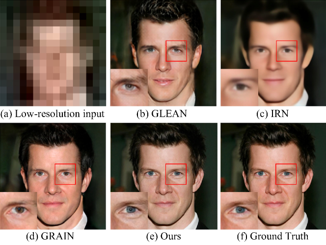
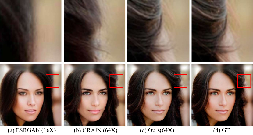
To further improve the reconstruction performance, recently developed invertible rescaling network (IRN) based and generative adversarial network (GAN) based methods Xiao et al. (2020); Zhong et al. (2022) have demonstrated impressive performance in image rescaling. Among them, IRN Xiao et al. (2020) transforms high-frequency components into a latent space, and assumes that the LR components and high-frequency components are independent. To consider the effect of the LR counterparts, HCFlow Liang et al. (2021) using a hierarchical conditional framework for modeling the LR information. Later, GRAIN Zhong et al. (2022) introduces a reciprocal invertible image rescaling approach, enabling subtle embedding of HR information into a reversible LR image and generative prior for accurate HR reconstruction. Despite the success of these generative methods in image rescaling, they still suffer from visually unpleasing results, due to the inaccurate modeling way of the high-frequency information. As shown in Fig. 1, existing methods produce over-smoothed results or fake details, thus leading to unrealistic results.
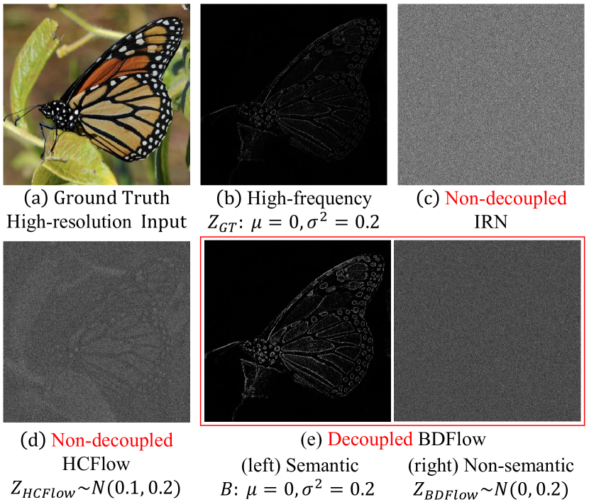
On the other hand, it is observed that the high-frequency part of the input deviates from a standard Gaussian distribution. As shown in Fig. 2(b), we compute the statistics of the high-frequency information from DIV2K and CelebA, which is obtained by computing the difference between the HR image in Fig. 2(a) and the reconstructed image of LR. We observe that is a mixture of semantic boundary information and Gaussian distribution with and . This motivates us to decouple the high-frequency information into different parts.
The above observations inspire us to design a more effective modeling way for high-frequency information, in this paper, we propose Decoupled Boundary-aware Decoupled Flow Networks (BDFlow), which decouples the original high-frequency information into approximate semantic Boundary distribution and non-semantic Gaussian distribution. As shown in Fig. 1(e), we utilize Boundary-aware Mask (BAM) to preserve semantic information, ensuring that the recovered image follows the true distribution. The non-semantic Gaussian distribution is independent of the low-frequency distribution and semantic Boundary distribution, and is randomly sampled in the backward process. Furthermore, we impose additional constraints on the model to generate textures consistent with the Ground Truth by utilizing the Boundary-aware Weight (BAW).
In summary, our main contributions are:
-
•
To our best knowledge, the proposed Boundary-aware Decoupled Flow Networks (BDFlow) is the first attempt to decouple high-frequency information into semantic Boundary distribution and non-semantic Gaussian distribution.
-
•
We introduce a general Boundary-aware Mask (BAM) to preserve semantic information, ensuring that the recovered image follows the true distribution. Canny operator is a special case of BAM, where the quantization is binarized, and the magnitude of the gradient is calculated using the 2-Norm. Additionally, our proposed Boundary-aware Weight (BAW) further constrains the model to generate rich texture details.
-
•
Extensive experiments demonstrate that our proposed BDFlow achieves state-of-the-art (SOTA) performance while maintaining a lower computational burden and faster inference time compared to other existing methods. We also explore and analyze image invertibility with respect to different influencing factors, such as scaling factor, JPEG compression, and data domain.
2 Related Work
2.1 Image Rescaling Methods
Image rescaling aims to downscale a high-resolution (HR) image to a visually pleasing low-resolution (LR) image and later reconstruct the HR image. In recent years, there has been a surge in the use of normalization flow Xiao et al. (2020); Liang et al. (2021); Li et al. (2024a) and generative adversarial network (GAN) Zhong et al. (2022); Chan et al. (2021); Yang et al. (2021) techniques for tackling the issue of image rescaling. IRN Xiao et al. (2020) transforms high-frequency information into a latent space which is a Gaussian distribution. Contrarily, HCFlowLiang et al. (2021) posits that the high-frequency information is dependent on the LR image. GANs-based GRAIN Zhong et al. (2022) introduces a reciprocal approach, enabling delicate embedding of high-resolution information into a reversible low-resolution image and generative prior. However, IRN generates overly smooth images due to the substantial loss of high-frequency information. HCFlow is non-decoupled and biased estimation. GRAIN produces fake details and requires extensive computation. To address these issues, we introduce light-weight Boundary-aware Mask (BAM) to constrain the model to produce rich textures.
2.2 Boundary-aware Methods
Boundary-aware techniques are vital for preserving facial structure and appearance in image rescaling, especially for facial images. These methods have proven effective in applications like face recognition and segmentation. Previous Boundary-aware work involves attention mechanisms Wang et al. (2017); Tang et al. (2024); Zhang et al. (2023), edge-aware filtering Xu et al. (2011); Chen et al. (2013); Li et al. (2024b), and facial landmark detection Cao et al. (2014); Kazemi and Sullivan (2014). Attention mechanisms focus on important features, improving recognition and segmentation. Edge-aware filtering preserves boundaries while maintaining smoothness elsewhere. Integrating Boundary-aware methods in image rescaling models offers advantages in preserving semantic Boundary distribution and model robustness.
2.3 Invertible Residual Networks
Initially developed for unsupervised learning of probabilistic models Behrmann et al. (2019); Dinh et al. (2016); Liu et al. (2020); Wang et al. (2023); Gao et al. (2023), Invertible Residual Networks (IRN) facilitate the transformation of one distribution to another through bijective functions, thereby preserving information integrity. This characteristic empowers invertible networks to ascertain the precise density of observations, which can subsequently be employed to generate images with intricate distributions. Owing to these distinctive properties, invertible networks have been effectively utilized in an array of applications, including image rescaling Xiao et al. (2020); Liang et al. (2021). In this work, we adopt the Invertible Residual Networks architecture presented in Dinh et al. (2016), which consists of a series of invertible blocks. For the block, the forward process is formulated as:
| (1) | ||||
Here, and represent arbitrary transformation functions. The input is decomposed into and . The backward process can be conveniently defined as:
| (2) | ||||
3 Methodology
3.1 Networks Framework
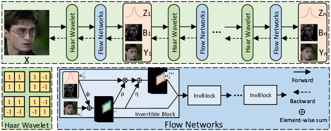
BDFlow can be dissected into three components: the Boundary-aware Mask generation algorithm (shown in Algorithm. 1), the Haar Wavelet transformation Lienhart and Maydt (2002), and the Flow Networks (shown in Fig. 3).
Image rescaling focuses on reconstructing a high-resolution (HR) image from a low-resolution (LR) image and high-frequency distribution, which are obtained by downscaling . As the downscaling process is the inverse of upscaling, we employ an invertible neural network to generate the LR image and decouple high-frequency distribution to non-semantic Gaussian distribution and semantic Boundary distribution (). Inversely, can be reconstructed through the inverse process from : . It is important to note that the Boundary distribution preserves semantic information in , and corresponds to the non-semantic high-frequency information, as per the Nyquist-Shannon sampling theorem Shannon (1949). To ensure the model’s invertibility, we must verify that is invertible, which is equivalent to having a non-zero determinant of the Jacobian for each invertible unit .
| (3) |
Here, and represent two transformations of each invertible unit. corresponds to , and corresponds to in Eq. 1. The value of is equal to due to .
3.2 Boundary-aware Decoupled Flow Networks
Boundary-aware Decoupled Flow Networks (BDFlow) decouple high-frequency information into non-semantic Gaussian distribution and semantic Boundary distribution. General Boundary-aware Mask preserves semantic information, ensuring that the recovered image follows the true distribution.
Boundary-aware Mask. The Boundary-aware Mask (BAM) is a crucial component of the BDFlow Networks, and its generation process can be summarized as follows. As shown in Algorithm 1, given an input image, denoted as , the algorithm begins by applying a Gaussian blur with a standard deviation of to produce a blurred image . Next, the gradient components and of the blurred image are computed, which are then used to calculate the gradient magnitude (1-Norm, 2-Norm or others). Subsequently, non-maximum suppression is performed on the gradient magnitude to obtain a thinned boundary map . The boundary map is then sparsified by applying a threshold , resulting in a sparse boundary map . Finally, the sparse boundary map is quantified to create the Boundary-aware Mask .
Canny operator is a special case of BAM, where the quantization is binarized, and the magnitude of the gradient is calculated using the 2-Norm.
Boundary-aware Weight. The proposed Boundary-aware Weight (BAW) further constrains the model to generate rich textures and semantic Boundary distribution, defined as:
| (4) |
where is a hyper-parameter, denotes 30 per cent of the training epochs, is the current training epoch and is the max training epoch. During the pre-training period (), the precision of the BAM is inadequate, and therefore fixed weights are employed. In the later training period, the in the BAM is utilized after normalization, and is used to weight the loss . The purpose of normalisation is to remove the effects of outliers. penalises the model for errors in the high-frequency textures of Ground Truth, constraining the model to generate a realistic Boundary distribution.
Input: , input image
Parameter: , the threshold to sparsify boundary
Output:
Haar Wavelet. We employ the Haar Wavelet (Other wavelet bases are discussed in the supplementary material.) transformation Mallat (1989) to decompose the input into high and low-frequency information, represented as . Specifically, given an HR image with shape , Haar Wavelet transformation decomposes into global frequency features :
| (5) | ||||
where denotes layer of the Flow Networks. and with shape and , correspond to low-frequency and high-frequency information, respectively.
Flow Networks. Subsequently, Flow Networks are employed to transform the frequency information into the semantic Boundary distribution, non-semantic Gaussian distribution, and LR distribution. Specifically, wavelet features and are fed into stacked InvBlocks to obtain the LR and high-frequency distribution . In our framework, is decoupled into semantic Boundary distribution and non-semantic Gaussian distribution . We adopt the general coupling layer for the invertible architecture Jacobsen et al. (2018); Behrmann et al. (2019). The output of each InvBlock can be defined as:
| (6) | ||||
where and are the outputs of the current InvBlock and the inputs of the next InvBlock. Notably, , , and are arbitrary transformation functions. We use the residual block He et al. (2016) to enhance the model’s nonlinear expressiveness and information transmission capabilities.
InvBlock extracts image features from and to and . After the transformation of InvBlocks, we obtain the downscaled image with dimensions , Boundary distribution with dimensions , and Gaussian distribution with dimensions .
3.3 Loss Function
Image rescaling aims to accurately reconstruct the HR image while generating visually pleasing LR images. Following IRN Xiao et al. (2020) and HCFlow Liang et al. (2021), we train our BDFlow by minimizing the following loss:
| (7) | ||||
where and are the ground-truth HR image and LR image, respectively. and are the ground-truth semantic Boundary distribution and non-semantic Gaussian distribution, respectively. is the reconstructed HR image from the generated LR image , Boundary distribution , and sampled Gaussian distribution .
is the pixel loss defined as:
| (8) |
where is the number of pixels, is the generated LR image, and is a hyper-parameter balancing different losses.
is the pixel loss defined as:
| (9) |
where is the number of pixels, , and is generated by the generation process of BAM but does not need to be quantified, which is in Algorithm 1 and Eq. 4.
with the weight is used to enhance the visual effect of the image generated by the model. Similarly, is the pixel loss defined as:
| (10) |
where is the number of pixels, is a hyper-parameter, and is the generated semantic Boundary distribution.
The last term, , chooses more stable distribution metrics for minimization to ensure that follows a non-semantic Gaussian distribution Xiao et al. (2020), defined as:
| (11) |
We jointly optimize the invertible architecture by utilizing both forward and backward losses.
4 Experiments
4.1 Datasets
We utilize the CelebA-HQ dataset Karras et al. (2020) to train our BDFlow. The dataset comprises 30,000 high-resolution () human face images. Moreover, we evaluate our models using widely-accepted pixel-wise metrics, including PSNR, SSIM, and LPIPS Zhang et al. (2018a) (Y channel) on the CelebA-HQ test dataset. We additionally train our BDFlow on the Cat dataset Zhang et al. (2008) and the LSUN-Church Yu et al. (2015) dataset to evaluate its generalization ability across different domains.
4.2 Training Details
Our BDFlow consists of Haar Wavelet Transformation and Flow Networks for , each containing two Invertible Blocks (InvBlocks). We train these models using the ADAM Kingma and Ba (2014) optimizer with and . Furthermore, we initialize the learning rate at and apply a cosine annealing schedule, decaying from the initial value to over the total number of iterations. We set , , , , and to 2, 2, 1, 16, and 4, respectively.
| Scale | Model | CelebA | ||
|---|---|---|---|---|
| PSNR | SSIM | LPIPS | ||
| Bicubic & DIC | 25.55 | 0.7574 | 0.5526 | |
| Bicubic & SRFlow | 26.74 | 0.7600 | 0.2160 | |
| HCFlow | 26.66 | 0.7700 | 0.2100 | |
| BDFlow (ours) | ||||
| Bicubic & WSRNet | 22.91 | 0.6201 | 0.5432 | |
| Bicubic & ESRGAN | 21.01 | 0.5959 | 0.4464 | |
| BDFlow (ours) | ||||
| GPEN | 20.40 | 0.5919 | 0.3714 | |
| IRN | 24.41 | 0.6943 | 0.5238 | |
| BDFlow (ours) | ||||
| PULSE | 19.20 | 0.5515 | 0.4867 | |
| pSp | 17.70 | 0.5590 | 0.4456 | |
| Bicubic & GLEAN | 20.24 | 0.6354 | 0.3891 | |
| Bicubic & Bilinear | 19.92 | 0.6840 | 0.6027 | |
| TAR | 25.15 | 0.7397 | 0.4733 | |
| GRAIN | 22.30 | 0.6467 | ||
| BDFlow (ours) | 0.3672 | |||
4.3 Comparison with State-of-the-art Methods
We compare our BDFlow with several state-of-the-art methods, including GAN-based inversion methods, CNN-based SR methods, and invertible rescaling methods. Table 1 presents the quantitative evaluations of the various approaches. Evidently, CNN-based methods outperform GAN-based methods in terms of PSNR and SSIM, as they tend to produce fuzzy results that follow the overall structure. Our flow-based approach BDFlow achieves superior PSNR and SSIM, with LPIPS results second only to GRAIN Zhong et al. (2022) on . This demonstrates that our model considers not only pixel-level fidelity but also perceptual visual effects in facilitating the decoupling of high-frequency information into semantic Boundary distribution and non-semantic Gaussian distribution. Specifically, BDFlow improves the PSNR by and the SSIM by on average over GRAIN.
Table 2 compares IRN Xiao et al. (2020), GRAIN Zhong et al. (2022), and our BDFlow in terms of model parameters, computational effort, and inference time. Our BDFlow surpasses IRN in all dimensions and outperforms GRAIN by using only 74% of the parameters and 20% of the computation. Notably, BDFlow is suitable for real-time applications, as it can achieve 100 fps.
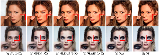
Fig. 4 contrasts our BDFlow with the GAN-based approach. In particular, pSp Richardson et al. (2021) recovers images of faces with different identities, while the results of GPEN Yang et al. (2021) and GLEAN Chan et al. (2021) display slight quality improvements but still exhibit significant flaws. Major differences persist in hair, eyebrows, eyes, and facial expressions. Although GRAIN Zhong et al. (2022) combines reversible and generative priors, it can only mitigate the limitation of under-informed input. GRAIN achieves good detail generation but produces some unfaithful details, as shown in Fig. 4 (d). In contrast, as shown in Fig. 4 (e), our BDFlow excels in both realism and fidelity, capturing semantic facial features, like vivid facial expressions, flyaway hair, and eye color.
| Scale | Model | Paras | FLOPs | Time |
|---|---|---|---|---|
| IRN | ||||
| BDFlow | ||||
| IRN | ||||
| BDFlow | ||||
| IRN | ||||
| BDFlow | ||||
| IRN | ||||
| GRAIN | ||||
| BDFlow |
4.4 Ablation Study
We conducted an ablation study to evaluate the impact of our proposed BAM and BAW. The effects of LPIPS loss, different Norm Loss, different wavelet bases, and hyper-parameters are discussed in the supplementary material.
| BAM | BAW | PSNR | SSIM | LPIPS |
| ✔ | ✗ | 26.06 | 0.7798 | 0.3673 |
| ✗ | ✔ | 25.03 | 0.7652 | 0.3823 |
| ✔ | ✔ |
| Quantify | Magnitude | T | PSNR | SSIM | LPIPS |
|---|---|---|---|---|---|
| 1 bit | 2-Norm | 20 | 26.09 | 0.7799 | 0.3681 |
| 1 bit | 2-Norm | 50 | |||
| 1 bit | 2-Norm | 100 | 26.11 | 0.7802 | 0.3675 |
| 1 bit | 1-Norm | 50 | 26.09 | 0.7798 | 0.3684 |
| 1 bit | 2-Norm | 50 | 26.12 | 0.7805 | 0.3672 |
| 2 bit | 2-Norm | 50 | 26.51 | 0.7913 | 0.3495 |
| 3 bit | 2-Norm | 50 |
Boundary Distribution and Semantic High-frequency Textures. Boundary-aware Mask (BAM) and Boundary-aware Weight (BAW) are able to recover more realistic Boundary distribution, such as the hair strands shown in Fig. 5 (c), because they focus on handling image boundaries and regions with high-frequency information more effectively. This is achieved by encouraging the model to decouple the high-frequency information into non-semantic Gaussian distribution and semantic Boundary distribution. However, GAN-based methods, like ESRGAN Wang et al. (2018) and GRAIN Zhong et al. (2022), generate fake details without the constraint of semantic Boundary distribution.
Table 3 demonstrates that the BDFlow structure incorporating both BAM and BAW consistently outperforms the basic BDFlow structure in terms of PSNR, SSIM, and LPIPS. Specifically, Table 4 shows that BAM with a threshold value of achieves superior performance due to the smaller values of high-frequency textures, which have a mean of approximately 50. Additionally, using the 2-Norm for magnitude calculation is better than using the 1-Norm because it widens the gap between different magnitudes. It is worth noting that the Canny operator can be regarded as a special case of BAM, where quantization is binarized and the magnitude of the gradient is calculated using the 2-Norm. However, as the level of quantization increases, the model achieves better performance. The Boundary distribution with 1 bit and single channel requires only a 4% () increase in storage cost, but can be further compressed to 1% due to the sparsity of high frequency.
4.5 Discussions
In our discussions, we conducted various analyses to evaluate the effectiveness of our approach. Firstly, we conducted a comparative analysis against the widely-used JPEG image compression technique to establish its superiority. Next, we evaluated the effect of BDFlow on different domains. More discussion is placed in the supplementary material, including the scale of sampled and evaluation of LR Images.
| Quality | Model | CelebA | |
|---|---|---|---|
| PSNR (dB) | Storage (B) | ||
| 1 | JPEG | 23.64 | 18803 |
| GRAIN | 22.30 | ||
| BDFlow | |||
| 5 | JPEG | 26.94 | 21511 |
| GRAIN | 25.60 | ||
| BDFlow | |||
| 10 | JPEG | 31.21 | 27933 |
| GRAIN | 28.13 | ||
| BDFlow | |||
| 40 | JPEG | 52979 | |
| GRAIN | 32.60 | ||
| BDFlow | 38.93 | ||
Comparison with JPEG Compression. Table 5 illustrates the superior performance of BDFlow compared to JPEG compression and GRAIN Zhong et al. (2022) in terms of PSNR and storage size. BDFlow consistently achieves higher PSNR values while maintaining storage sizes comparable to GRAIN, showcasing its ability to effectively compress images while preserving the quality of the reconstructed images. BDFlow’s decoupling of high-frequency information into semantic Boundary distribution and non-semantic Gaussian distribution is at the core of the above gains. In addition, JPEG compression and rescaling are not in conflict, it is possible to continue to compress images using the JPEG algorithm after rescaling.
| Domain | Model | PSNR | SSIM |
|---|---|---|---|
| Cat | GRAIN () | 21.97 | 0.5250 |
| BDFlow () | |||
| Church | GRAIN () | 18.48 | 0.4421 |
| BDFlow () | |||
| Set5 | GRAIN () | 22.33 | 0.7718 |
| BDFlow () | |||
| Set14 | GRAIN () | 19.96 | 0.6055 |
| BDFlow () | |||
| B100 | GRAIN () | 21.56 | 0.6128 |
| BDFlow () | |||
| Urban100 | GRAIN () | 16.77 | 0.3886 |
| BDFlow () | |||
| DIV2K | GRAIN () | 19.03 | 0.4901 |
| BDFlow () |
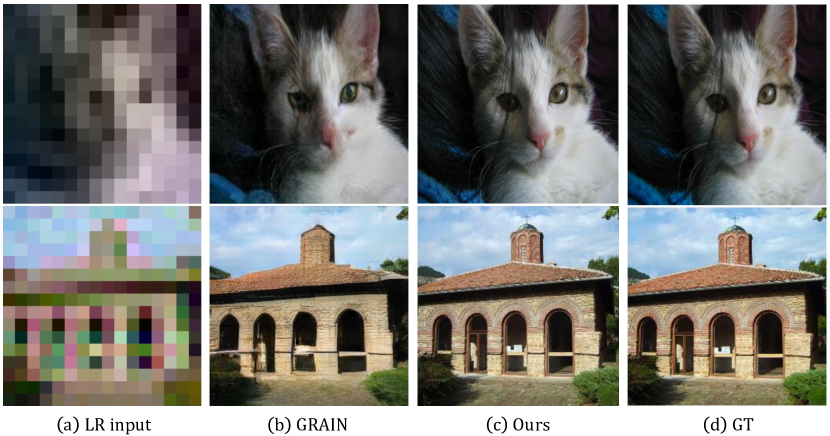
Evaluation in Different Domains. As shown in Fig. 6 and Table 6, we evaluate our proposed approach in different Domains. These experiments demonstrate the generalisation ability of our proposed BDFlow in reconstructing images from different Domains. This is attributed to the fact that we decouple the true high-frequency distributions into semantic Boundary distribution and non-semantic Gaussian distribution, which helps to achieve the final realistic results. As shown in Fig. 6, GRAIN has difficulty recovering the hair of the cat and the edges of the church, but our BDFlow is able to do so with high fidelity. As shown in Table 6, our BDFlow achieves much higher PSNR and SSIM than GRAIN at the pixel level.
Loss and Loss. We use loss and loss in some cases in our method for the fairness comparison, since we followed the default setup of the previous works Xiao et al. (2020); Liang et al. (2021). Besides, we have conducted experiments to verify the effects of Norm-loss (see in Table 1 of the Supplementary Material). In fact, the forward process utilizes to increase the penalty for outliers in favor of constraining the LR distribution, Gaussian distribution, and Boundary distribution. The backward process utilizes the loss encouraging the model to recover more detail rather than smoothing the image, thus leading to better LPIPS. Thus, may be a proper choice.
5 Conclusion
In this paper, we proposed the Boundary-aware Decoupled Flow Networks (BDFlow), which decouple high-frequency information into non-semantic Gaussian distribution and semantic Boundary distribution. This approach effectively preserves boundary information and texture details in the image rescaling process. Specifically, by introducing a generated Boundary-aware Mask, our model ensures that the recovered image follows the true high-frequency distribution and generates rich semantic details. Boundary-aware Mask further constrains the generation of the model to obey the true semantic distribution.
6 Acknowledgements
This work is supported in part by the National Natural Science Foundation of China, under Grant (62302309, 62171248), Shenzhen Science and Technology Program (JCYJ20220818101014030, JCYJ20220818101012025), and the PCNL KEY project (PCL2023AS6-1), and Tencent “Rhinoceros Birds” - Scientific Research Foundation for Young Teachers of Shenzhen University.
References
- Behrmann et al. [2019] Jens Behrmann, Will Grathwohl, Ricky TQ Chen, David Duvenaud, and Jörn-Henrik Jacobsen. Invertible residual networks. In International Conference on Machine Learning, pages 573–582. PMLR, 2019.
- Cao et al. [2014] Xudong Cao, Yichen Wei, Fang Wen, and Jian Sun. Face alignment by explicit shape regression. International journal of computer vision, 107:177–190, 2014.
- Chan et al. [2021] Kelvin CK Chan, Xintao Wang, Xiangyu Xu, Jinwei Gu, and Chen Change Loy. Glean: Generative latent bank for large-factor image super-resolution. In Proceedings of the IEEE/CVF conference on computer vision and pattern recognition, pages 14245–14254, 2021.
- Chen et al. [2013] Qifeng Chen, Dingzeyu Li, and Chi-Keung Tang. Knn matting. IEEE transactions on pattern analysis and machine intelligence, 35(9):2175–2188, 2013.
- Cui et al. [2023] Yuning Cui, Wenqi Ren, Xiaochun Cao, and Alois Knoll. Image restoration via frequency selection. IEEE Transactions on Pattern Analysis and Machine Intelligence, 2023.
- Dai et al. [2023] Tao Dai, Mengxi Ya, Jinmin Li, Xinyi Zhang, Shu-Tao Xia, and Zexuan Zhu. Cfgn: A lightweight context feature guided network for image super-resolution. IEEE Transactions on Emerging Topics in Computational Intelligence, 2023.
- Dinh et al. [2016] Laurent Dinh, Jascha Sohl-Dickstein, and Samy Bengio. Density estimation using real nvp. arXiv preprint arXiv:1605.08803, 2016.
- Dong et al. [2014] Chao Dong, Chen Change Loy, Kaiming He, and Xiaoou Tang. Learning a deep convolutional network for image super-resolution. In European conference on computer vision, pages 184–199. Springer, 2014.
- Gao et al. [2023] Kuofeng Gao, Yang Bai, Jindong Gu, Yong Yang, and Shu-Tao Xia. Backdoor defense via adaptively splitting poisoned dataset. In CVPR, 2023.
- Guo et al. [2024] Hang Guo, Jinmin Li, Tao Dai, Zhihao Ouyang, Xudong Ren, and Shu-Tao Xia. Mambair: A simple baseline for image restoration with state-space model. arXiv preprint arXiv:2402.15648, 2024.
- He et al. [2016] Kaiming He, Xiangyu Zhang, Shaoqing Ren, and Jian Sun. Deep residual learning for image recognition. In Proceedings of the IEEE conference on computer vision and pattern recognition, pages 770–778, 2016.
- Jacobsen et al. [2018] Jörn-Henrik Jacobsen, Arnold Smeulders, and Edouard Oyallon. i-revnet: Deep invertible networks. arXiv preprint arXiv:1802.07088, 2018.
- Karras et al. [2020] Tero Karras, Samuli Laine, Miika Aittala, Janne Hellsten, Jaakko Lehtinen, and Timo Aila. Analyzing and improving the image quality of stylegan. In Proceedings of the IEEE/CVF conference on computer vision and pattern recognition, pages 8110–8119, 2020.
- Kazemi and Sullivan [2014] Vahid Kazemi and Josephine Sullivan. One millisecond face alignment with an ensemble of regression trees. In Proceedings of the IEEE conference on computer vision and pattern recognition, pages 1867–1874, 2014.
- Kingma and Ba [2014] Diederik P Kingma and Jimmy Ba. Adam: A method for stochastic optimization. arXiv preprint arXiv:1412.6980, 2014.
- Li et al. [2023] Jinmin Li, Tao Dai, Mingyan Zhu, Bin Chen, Zhi Wang, and Shu-Tao Xia. Fsr: A general frequency-oriented framework to accelerate image super-resolution networks. In Proceedings of the AAAI Conference on Artificial Intelligence, volume 37, pages 1343–1350, 2023.
- Li et al. [2024a] Jinmin Li, Tao Dai, Yaohua Zha, Yilu Luo, Longfei Lu, Bin Chen, Zhi Wang, Shu-Tao Xia, and Jingyun Zhang. Invertible residual rescaling models. arXiv preprint arXiv:2405.02945, 2024.
- Li et al. [2024b] Jinmin Li, Kuofeng Gao, Yang Bai, Jingyun Zhang, Shu-tao Xia, and Yisen Wang. Fmm-attack: A flow-based multi-modal adversarial attack on video-based llms. arXiv preprint arXiv:2403.13507, 2024.
- Liang et al. [2021] Jingyun Liang, Andreas Lugmayr, Kai Zhang, Martin Danelljan, Luc Van Gool, and Radu Timofte. Hierarchical conditional flow: A unified framework for image super-resolution and image rescaling. In Proceedings of the IEEE/CVF International Conference on Computer Vision (ICCV), pages 4076–4085, October 2021.
- Lienhart and Maydt [2002] Rainer Lienhart and Jochen Maydt. An extended set of haar-like features for rapid object detection. In Proceedings. international conference on image processing, volume 1, pages I–I. IEEE, 2002.
- Lim et al. [2017] Bee Lim, Sanghyun Son, Heewon Kim, Seungjun Nah, and Kyoung Mu Lee. Enhanced deep residual networks for single image super-resolution. In Proceedings of the IEEE conference on computer vision and pattern recognition workshops, pages 136–144, 2017.
- Liu et al. [2020] Yang Liu, Zhenyue Qin, Saeed Anwar, Sabrina Caldwell, and Tom Gedeon. Are deep neural architectures losing information? invertibility is indispensable. In Neural Information Processing: 27th International Conference, ICONIP 2020, Bangkok, Thailand, November 23–27, 2020, Proceedings, Part III 27, pages 172–184. Springer, 2020.
- Mallat [1989] Stephane G Mallat. A theory for multiresolution signal decomposition: the wavelet representation. IEEE transactions on pattern analysis and machine intelligence, 11(7):674–693, 1989.
- Richardson et al. [2021] Elad Richardson, Yuval Alaluf, Or Patashnik, Yotam Nitzan, Yaniv Azar, Stav Shapiro, and Daniel Cohen-Or. Encoding in style: a stylegan encoder for image-to-image translation. In Proceedings of the IEEE/CVF conference on computer vision and pattern recognition, pages 2287–2296, 2021.
- Shannon [1949] Claude E Shannon. Communication in the presence of noise. Proceedings of the IRE, 37(1):10–21, 1949.
- Tang et al. [2024] Xiaolong Tang, Meina Kan, Shiguang Shan, Zhilong Ji, Jinfeng Bai, and Xilin Chen. Hpnet: Dynamic trajectory forecasting with historical prediction attention. arXiv preprint arXiv:2404.06351, 2024.
- Wang et al. [2017] Fei Wang, Mengqing Jiang, Chen Qian, Shuo Yang, Cheng Li, Honggang Zhang, Xiaogang Wang, and Xiaoou Tang. Residual attention network for image classification. In Proceedings of the IEEE conference on computer vision and pattern recognition, pages 3156–3164, 2017.
- Wang et al. [2018] Xintao Wang, Ke Yu, Shixiang Wu, Jinjin Gu, Yihao Liu, Chao Dong, Yu Qiao, and Chen Change Loy. Esrgan: Enhanced super-resolution generative adversarial networks. In Proceedings of the European conference on computer vision (ECCV) workshops, pages 0–0, 2018.
- Wang et al. [2023] Yuting Wang, Jinpeng Wang, Bin Chen, Ziyun Zeng, and Shu-Tao Xia. Contrastive masked autoencoders for self-supervised video hashing. In Proceedings of the AAAI Conference on Artificial Intelligence, volume 37, pages 2733–2741, 2023.
- Xiao et al. [2020] Mingqing Xiao, Shuxin Zheng, Chang Liu, Yaolong Wang, Di He, Guolin Ke, Jiang Bian, Zhouchen Lin, and Tie-Yan Liu. Invertible image rescaling. In Computer Vision–ECCV 2020: 16th European Conference, Glasgow, UK, August 23–28, 2020, Proceedings, Part I 16, pages 126–144. Springer, 2020.
- Xu et al. [2011] Li Xu, Cewu Lu, Yi Xu, and Jiaya Jia. Image smoothing via l 0 gradient minimization. In Proceedings of the 2011 SIGGRAPH Asia conference, pages 1–12, 2011.
- Yang et al. [2021] Tao Yang, Peiran Ren, Xuansong Xie, and Lei Zhang. Gan prior embedded network for blind face restoration in the wild. In Proceedings of the IEEE/CVF Conference on Computer Vision and Pattern Recognition, pages 672–681, 2021.
- Yu et al. [2015] Fisher Yu, Ari Seff, Yinda Zhang, Shuran Song, Thomas Funkhouser, and Jianxiong Xiao. Lsun: Construction of a large-scale image dataset using deep learning with humans in the loop. arXiv preprint arXiv:1506.03365, 2015.
- Zhang et al. [2008] Weiwei Zhang, Jian Sun, and Xiaoou Tang. Cat head detection-how to effectively exploit shape and texture features. In Computer Vision–ECCV 2008: 10th European Conference on Computer Vision, Marseille, France, October 12-18, 2008, Proceedings, Part IV 10, pages 802–816. Springer, 2008.
- Zhang et al. [2018a] Richard Zhang, Phillip Isola, Alexei A Efros, Eli Shechtman, and Oliver Wang. The unreasonable effectiveness of deep features as a perceptual metric. In Proceedings of the IEEE conference on computer vision and pattern recognition, pages 586–595, 2018.
- Zhang et al. [2018b] Yulun Zhang, Kunpeng Li, Kai Li, Lichen Wang, Bineng Zhong, and Yun Fu. Image super-resolution using very deep residual channel attention networks. In Proceedings of the European conference on computer vision (ECCV), pages 286–301, 2018.
- Zhang et al. [2023] Aiping Zhang, Wenqi Ren, Yi Liu, and Xiaochun Cao. Lightweight image super-resolution with superpixel token interaction. In Proceedings of the IEEE/CVF International Conference on Computer Vision, pages 12728–12737, 2023.
- Zhong et al. [2022] Zhixuan Zhong, Liangyu Chai, Yang Zhou, Bailin Deng, Jia Pan, and Shengfeng He. Faithful extreme rescaling via generative prior reciprocated invertible representations. In Proceedings of the IEEE/CVF Conference on Computer Vision and Pattern Recognition, pages 5708–5717, 2022.