MHD Modeling of the Molecular Filament Evolution
Abstract
We perform numerical magnetohydrodynamic (MHD) simulations of the gravitational collapse and fragmentation of a cylindrical molecular cloud with the help of the FLASH code. The cloud collapses rapidly along its radius without any signs of fragmentation in the simulations without magnetic field. The radial collapse of the cloud is stopped by the magnetic pressure gradient in the simulations with parallel magnetic field. Cores with high density form at the cloud’s ends during further evolution. The core densities are and cm-3 in the cases with initial magnetic field strengths and G, respectively. The cores move toward the cloud’s center with supersonic speeds and kms-1. The sizes of the cores along the filaments radius and filament’s main axis are pc and pc, pc and pc, respectively. The masses of the cores increase during the filament evolution and lie in range of . According to our results, the cores observed at the edges of molecular filaments can be a result of the filament evolution with parallel magnetic field.
Keywords: magnetic fields, magnetohydrodynamics (MHD), methods: numerical, ISM: clouds
Introduction
Modern observations show that interstellar clouds have a filamentary structure, which is traced from HI super clouds to individual molecular clouds Andre et. al. (2014). Filaments appear as elongated structures in the radiation maps of the interstellar medium. Such filaments can be either cylindrical clouds or edge-on sheets of molecular gas Dudorov & Khaibrakhmanov (2017). Most protostellar clouds in which star formation occurs are located within filamentary molecular clouds Konyves et. al. (2015). Therefore, the study of the structure and evolution of molecular filaments is important for the theory of star formation.
Observations show that the typical width of molecular filaments is of pc, and their length varies from several pc to hundreds of pc. The temperature in the filaments ranges from to K, and the gas density ranges from up to cm-3 Dudorov & Khaibrakhmanov (2017).
Polarization mapping of molecular clouds revealed the presence of large-scale magnetic fields Ward-Thompson et. al (2017). The magnetic field is usually aligned with the main axis of the filament in low density clouds, and it is perpendicular to the cloud’s axis in high density clouds. Measurements of the Zeeman splitting of OH lines and estimations with the Chandrasekhar-Fermi method showed that the strength of the magnetic field in the filaments increases with the column density and lies in the range from G for low density clouds with cm-2 to G for the dense filaments with cm-2.
The question of the nature of the filamentary structure of the interstellar medium is currently open Hacar et. al. (2023). Several mechanisms of the filament formation have been proposed in application to the various levels of the hierarchy of the interstellar medium: Parker and thermal instabilities on the scales of the spiral arms of the Galaxy, gravitational instability, collisions of interstellar shock waves in a turbulent medium, and large-scale anisotropic motions of the gas in the interstellar medium with magnetic field. The evolution of filaments after their formation depends on their initial state and external conditions.
Gravitational focusing results in the formation of dense cores at the ends of isolated homogeneous isothermal filaments. This mechanism is called as "end-dominated collapse Bastien (1983)" or "edge fragmentation Hacar et. al. (2023)". An example of such a cloud is the S242 filament, at the ends of which the cores with density of the order of cm-3 and the size of pc are observed Dewanghan et. al (2019).
Small longitudinal perturbations of the filaments can lead to the development of gravitational instability Chandrasekhar & Fermi (1953); Stodolkiewicz (1963); Ostriker (1964). In the case of filaments without magnetic field, instability develops for the perturbations with a wavelength 4 times larger than the radius of the homogeneous part of the filament. Instability leads to the formation of gravitational "sausages" and, subsequently, cores, which are distributed along the filament with a characteristic distance between them of the order of the fastest growing mode. The shape of the cores formed as a result of the gravitational fragmentation is close to spherical Inutsuka & Miyama (1997). The NGC 2024S/Orion B filament is an example of an object, in which signs of gravitational fragmentation are observed. Cores in this filament have sizes of the order of pc and masses of Shimajiri et. al (2023). The velocity profile along the filament is periodic with wavelength of pc. The cores are spatially shifted relative to the velocity spikes by , which indicates the gravitational fragmentation of the filament. Another example of such a filament is WB 673 Ryabukhina et. al. (2022).
Simulations of the filament fragmentation with magnetic field are necessary for the interpretation of the observational data. Seifried and Walch Seifried & Walch (2015) used the numerical code FLASH to simulate the evolution of filaments with turbulence and different magnetic field orientations. The authors identified several modes of filament fragmentation depending on the initial conditions: fragmentation at the ends, gravitational fragmentation of the filament with the subsequent formation of evenly distributed cores, and global collapse of the filament towards the center of the cloud. The authors showed that the pressure gradient of the parallel magnetic field maintains almost constant filament width of the order of 0.1 pc. Subsequently, this conclusion was confirmed in the MHD simulations by Dudorov and Khaibrakhmanov Dudorov & Khaibrakhmanov (2017).
In this work, numerical simulations of the homogeneous molecular filaments with parallel magnetic field is performed and the properties of the cores formed as a result of fragmentation at the edges of the filament are determined. The main attention is paid to the influence of the magnetic field on the fragmentation, as well as on the internal structure, size and mass of the resulting cores.
Section 1 describes the problem statement, the basic equations, and the numerical code FLASH, which is used to solve the equations. Subsection 2.2.1 presents the results of the simulation of the filament evolution without magnetic field and with weak magnetic field. The results of the simulations with stronger magnetic field are given in Subsection 2.2.2. Subsection 2.2.3 describes the characteristics of cores formed in the simulations with magnetic field. In summary, we outline and discuss our main results.
1 Model
1.1 Problem Statement
In this work, we simulate the gravitational collapse of a cylindrical molecular cloud (filament) with length pc and radius pc. The molecular weight of the gas is , temperature K, concentration cm-3. The filament mass-per-length pc-1 exceeds the critical value pc-1 Stodolkiewicz (1963); Ostriker (1964). Therefore, the filament is gravitationally unstable. Collapse simulations, which take into account radiation transfer, showed that the thermal energy of the compressed gas is effectively released and the gas temperature remains approximately constant in the concentration range cm-3. Therefore, for simplicity, we assume that the gas is characterized by the equation of state with the effective adiabatic index corresponding to the isothermal compression. The corresponding ratio of the cloud’s thermal energy to the absolute value of its gravitational energy is . The speed of sound in the filament is kms-1.
To study the role of the magnetic field in the evolution of filaments, we performed three simulations with different ratios of the cloud’s magnetic energy to the absolute value of its gravitational energy: (run ’HD’), (run ’MHD-1’), (run ’MHD-2’). Corresponding magnetic field strengths are G, respectively. The magnetic field is parallel to the filament’s axis in both cases. The filament is in pressure equilibrium with the external environment with concentration cm-3 and temperature K. The free fall time for the chosen density is years.
Let us find out whether it is necessary to take into account the magnetic diffusion when studying the initial stages of the filament collapse. To do this, we need to estimate the magnetic Reynolds number,
| (1) |
where and are typical gas velocity and spatial scales, and is the magnetic diffusivity. We choose the filament radius as the and the characteristic speed as .
Magnetic flux dissipation can be caused either by Ohmic dissipation (OD) or by magnetic ambipolar diffusion (MAD). We use the equations from Dudorov & Khaibrakhmanov (2014) to estimate the corresponding diffusivities
| (2) |
where is the ionization fraction, is the gas temperature, is the magnetic field strength, is the gas density, is the coefficient of the interaction between ions with mass and neutrals with mass , where , is the mass of the hydrogen atom
In the considered range of densities, the ionization fraction can be estimated from the balance of the ionization by cosmic rays with rate and radiative recombinations: , where is the coefficient of radiative recombinations, is the gas concentration Dudorov & Sazonov (1987).
Using typical parameters for the interstellar medium, we find for the case of Ohmic dissipation:
| (3) |
for ambipolar diffusion:
| (4) |
1.2 Basic Equations and Solution Methods
We study the evolution of the molecular filament using the system of ideal MHD equations:
| (5) | |||||
| (6) | |||||
| (7) | |||||
| (8) | |||||
| (9) | |||||
| (10) |
where , and are the density, velocity vector and pressure of the gas, is the gravitational potential, is the magnetic induction, is the internal energy of the gas, is the gravitational constant.
To simulate the evolution of the filament, we use the numerical code FLASH 4, in which the adaptive mesh refinement (AMR) technology is implemented Fryxell et. al. (2018). The equations of ideal MHD (5–8) are solved using the Godunov-type MUSCL scheme van Leer (1979). We consider a 3D problem in Cartesian coordinates. The -axis corresponds to the symmetry axis of the filament. The sizes of the computational domain in the -, -, and -directions are pc3, and 7 levels of the AMR grid are used. The sizes of the largest cell in the -, -, and -directions are pc3, the sizes of the smallest cells are pc3, which corresponds to the effective grid resolution at the 7th AMR level. The Poisson’s equation for gravity is solved using the multipole method based on the Barnes-Hut tree Barnes & Hut (1986).
2 Results
2.1 General Picture of the Filament’s Evolution
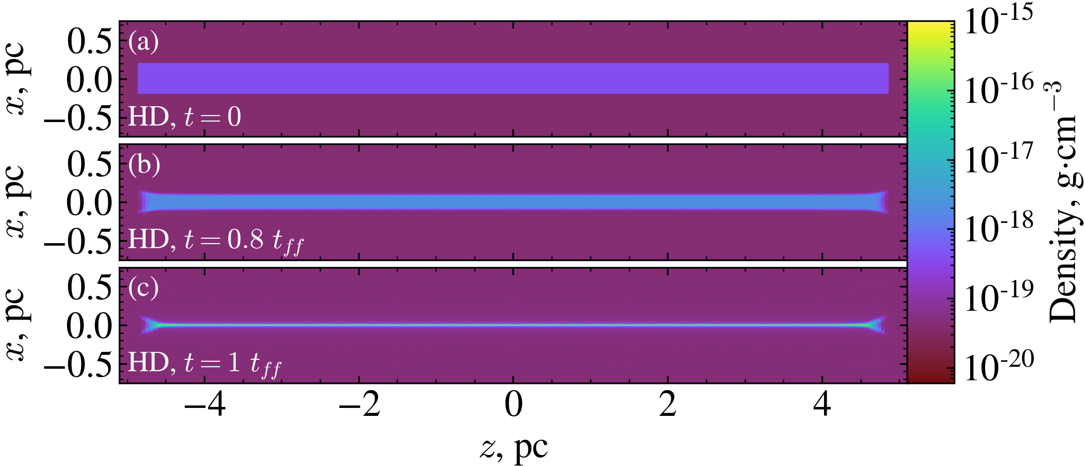
In Figure 1, we plot the gas density distribution in the plane for run ’HD’ at . The simulations show that non-magnetic filament freely collapses along the radius and the density at the center of the filament increases by 3 orders of magnitude by the time , the filament width along its radius is pc. The filament does not fragment.
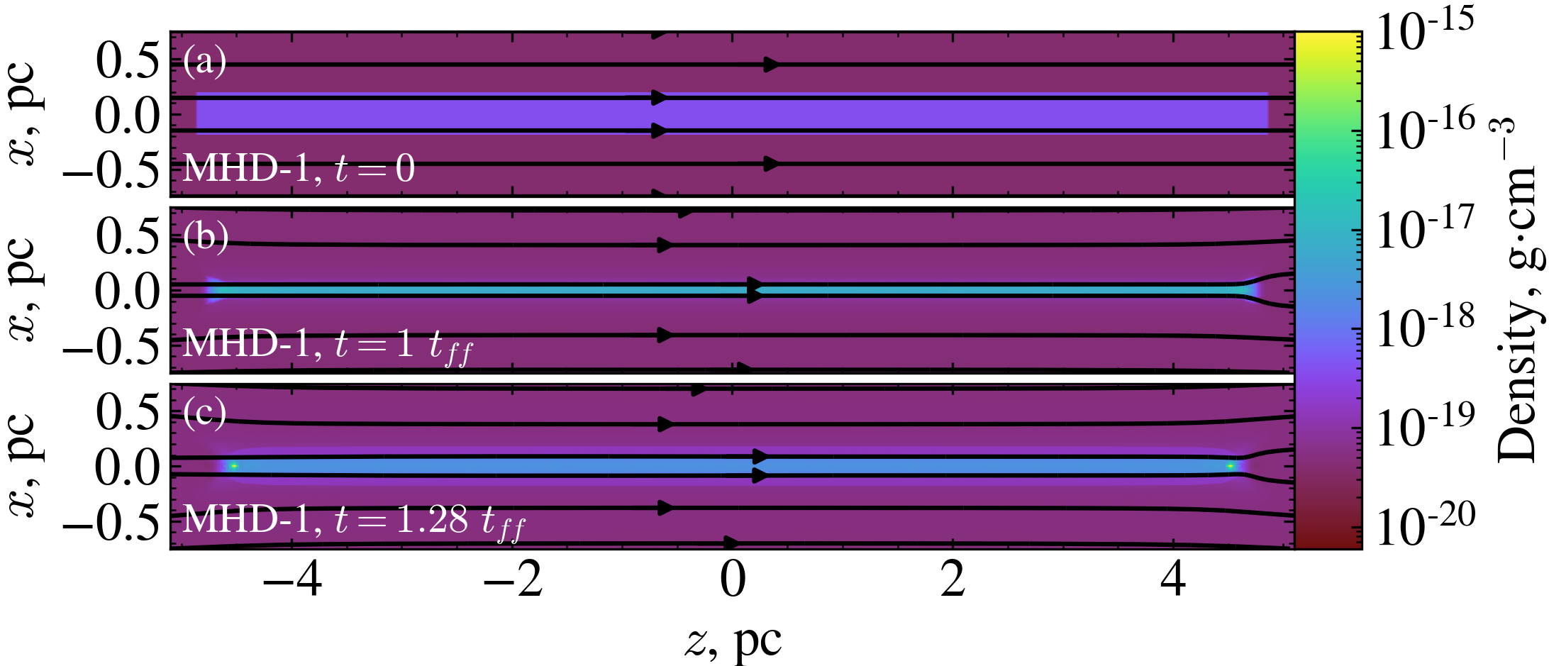
In Figure 2, we plot the gas density distribution in the plane for run ’MHD-1’ at . Figure 2 shows that the magnetic filament collapses to radius pc and density cm-3 by the time of . After that, the effective adiabatic index increases from to due to the action of the electromagnetic force, the collapse along is stopped by the magnetic pressure gradient, and the cloud starts to oscillate along the radius. Two cores with density cm-3 form at the edges of the cloud by the time . The properties of the cores are discussed further in the section "Characteristics of forming cores".
2.2 Influence of the Magnetic Field on the Evolution
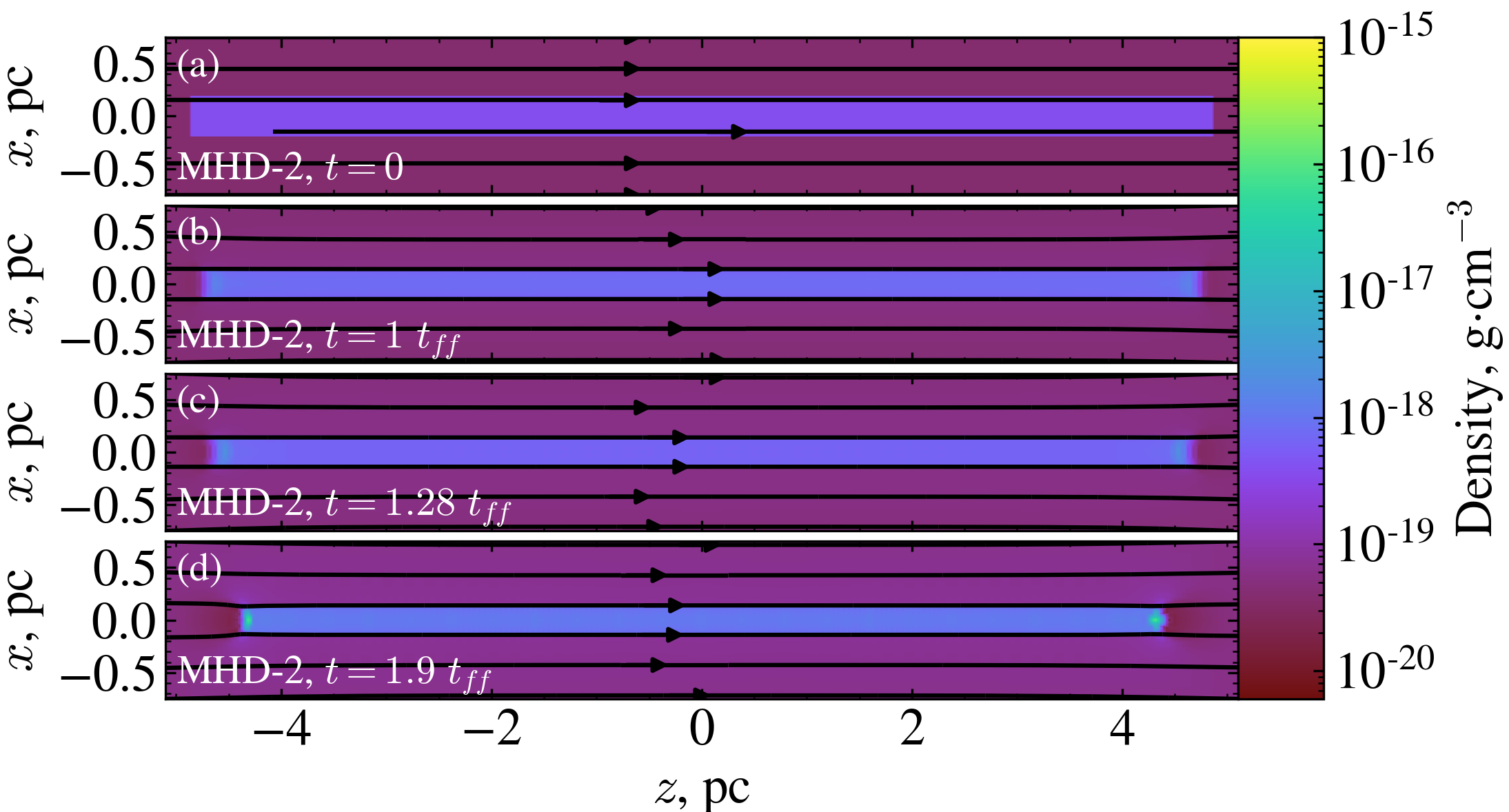
In Figure 3, we plot the gas density distribution in the -plane for run ’MHD-2’ at . In this run, the picture of the collapse is qualitatively similar to the results for run ’MHD-1’. The filament collapses to radius of pc and concentration of cm-3 at time , after which the collapse stops and the filament oscillates along the radius. The density of the cores formed at the ends of the filament is cm-3 at the time .
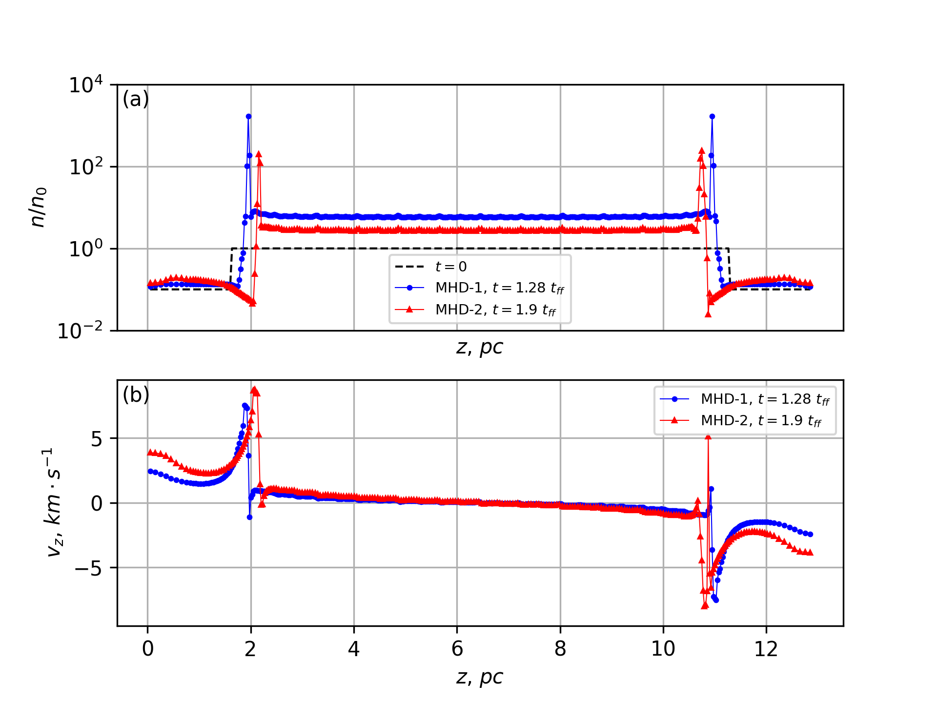
In Figure 4, we show the evolution of the density and velocity profiles along the filament’s axis in MHD runs. The filament edges are located at pc and pc initially. Figure 4 shows that, in run MHD-1, peaks densities cm-3 and velocities kms-1 are observed at the ends of the filament ( pc and pc) at the moment of time . These peaks correspond to the cores formed at the ends of the filament. The speed of the left core is positive, the speed of the right one is negative. Corresponding Mach number is , that is, the cores move at supersonic speeds towards each other.
In run MHD-2, the densities and velocities of the cores located at pc and pc at the time moment are equal to cm-3 and kms-1, respectively, and the corresponding Mach number is equal to .
2.3 Characteristics of Forming Cores
In Figure 5, we plot the distribution of gas density, magnetic field lines and velocity field for run MHD-1 in the region of core formation in the plane. Two moments of time are presented: and . Due to symmetry, only the core located at the "left" end of the filament is shown. In 6, we plot similar distribution for run MHD-2 at moments of time and in the -plane
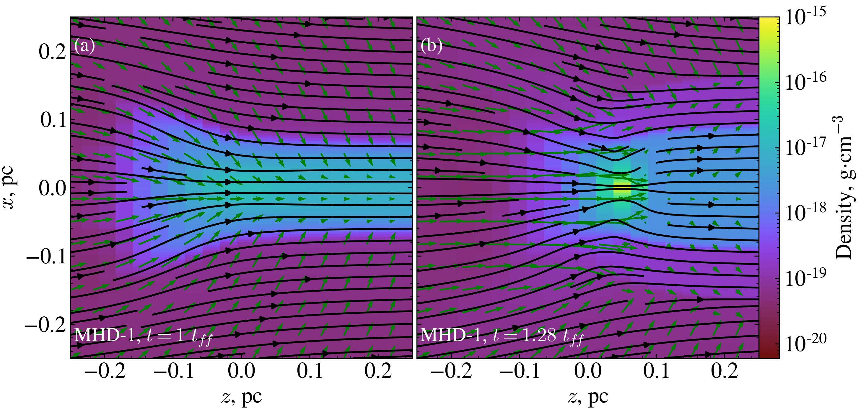
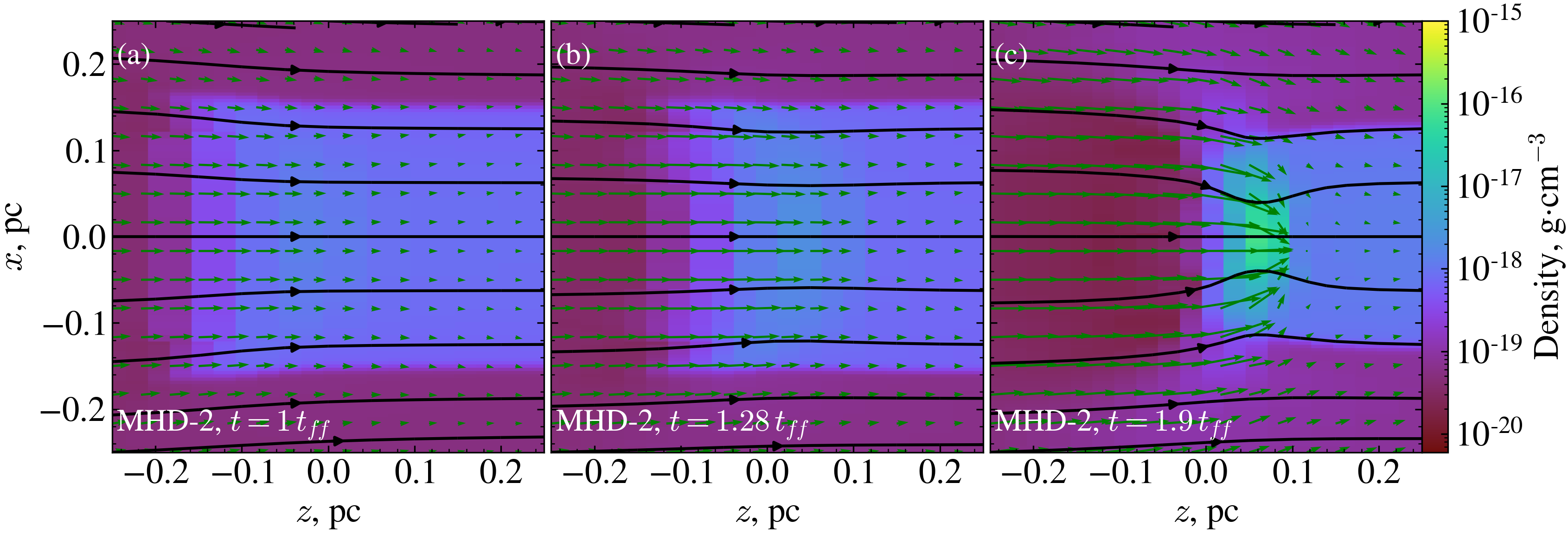
Table LABEL:Table_I: gives the following characteristics of the cores formed in MHD runs: sizes along the filament radius and the -axis (columns 3 and 4), concentration (column 5), mass (column 6) and velocity (column 7). The table shows that the cores of larger radius and lower density are formed in the simulation with larger magnetic field strength. This is due to the fact that the influence of the magnetic pressure gradient on the dynamics of the filament is increased in the case of stronger magnetic field. The sizes of the cores along the -axis do not depend on the strength of the initial magnetic field, since the parallel magnetic field does not prevent collapse of the filament along its axis. The masses of the cores grows as they move and reach in run MHD-1 and in run MHD-2.
| Run | Time, | , pc | , pc | , cm-3 | , | , kms-1 |
|---|---|---|---|---|---|---|
| (1) | (2) | (3) | (4) | (5) | (6) | (7) |
| MHD-1 | 1.28 | 0.0075 | 0.025 | |||
| MHD-2 | 1.28 | |||||
| 1.9 | 23.6 |
Summary
The influence of the magnetic field on the evolution of molecular filament and the characteristics of the cores formed in the filament as a result of end dominated collapse is investigated in this work. For this purpose, we performed a set of numerical MHD simulations of the gravitational collapse of a cylindrical molecular filament with different values of the parallel magnetic field.
Our simulations confirm the conclusions of earlier studies that the filament without magnetic field collapses freely along its radius. Fragmentation of the filament and the formation of the cores at its ends do not occur during the collapse, since the collapse along the radius occurs on a shorter time scale.
The magnetic pressure gradient prevents collapse and leads to decaying oscillations of the filament along its radius. During the evolution of magnetic filaments, dense clumps (cores) form at the ends of the filament due to the gravitational focusing. The cores move towards the center of the cloud at supersonic speeds of to kms-1. The clouds with stronger magnetic field are characterized by the formation of the cores of larger sizes and lower density, since the influence of the magnetic field pressure gradient along the radius increases with increasing magnetic field strength. The masses of the cores increase during the evolution of the filament and lie in the range .
Our simulations indicate that the end-dominated collapse is a natural result of the evolution of the filaments with parallel magnetic field. It can be assumed that the observed filaments with clumps located at ends (e.g., Dewanghan et. al (2019)) are supported from gravitational fragmentation by parallel magnetic field. Additional support against gravity can be provided by turbulence within the filament Seifried & Walch (2015); Federrath et. al. (2021).
We plan to further develop the presented model and model the evolution of initially non-uniform filaments taking into account their rotation and/or internal turbulence. It is of particular interest to study the fragmentation of the filament with parallel magnetic field due to the gravitational instability as described by the theory of Chandrasekhar and Fermi Chandrasekhar & Fermi (1953).
Acknowledgements.
The work is financially supported by the Foundation for Perspective Research of the Chelyabinsk State University (project 2023/7). The work by S.A. Khaibrakhmanov is supported by the Russian Ministry of Science and Higher Education via the Project FEUZ-2020-0038. The simulations were carried out using the computational cluster of the Chelyabinsk State University.References
- Andre et. al. (2014) Andre P., Di Francesco J., Ward-Thompson D., Inutsuka S. I., Pudritz R. E., Pineda J. E., 2014, Protostars and Planets VI, 27
- Dudorov & Khaibrakhmanov (2017) Dudorov A. E., Khaibrakhmanov S. A. 2017, Open Astronomy, 26, 285
- Konyves et. al. (2015) Konyves V., Andre Ph., Men’shchikov A., Palmeirim P., Arzoumanian D., Schneider N., Roy A., Didelon P., Maury A., Shimajiri Y., Di Francesco J., Bontemps S., Peretto N., Benedettini M., Bernard J. Ph., Elia D., Griffin M. J., Hill T., Kirk J., Ladjelate B., 2015, Astronomy and Astrophysics, 584, 33
- Ward-Thompson et. al (2017) Ward-Thompson D., Pattle K., Bastien P., Furuya R. S., Kwon W., Lai S. P., Qiu K., Berry D., Choi M., Coude S., Di Francesco J., Hoang T., Franzmann E., Friberg P., Graves S. F., Greaves J. S., Houde M., Johnstone D., Kirk J. M., Koch P. M. 2017, The Astrophysical Journal, 842, 10
- Hacar et. al. (2023) Hacar A., Clark S. E., Heitsch F., Kainulainen J., Panopoulou G. V, Seirfried D., Smith R., 2023, Protostars and Planets VII, ASP Conference Series, Proceedings of a conference, 534, 153
- Bastien (1983) Bastien P., 1983, Astronomy and Astrophysics, 119, 109
- Dewanghan et. al (2019) Dewangan L. K, Pirogov L. E., Ryabukhina O. L., Ojha D. K., Zinchenko I., 2019, The Astrophysical Journal, 877, 1
- Chandrasekhar & Fermi (1953) Chandrasekhar S., Fermi E., 1953, Astrophysical journal, 118, 116
- Stodolkiewicz (1963) Stodolkiewicz J. S, 1963, Acta Astronomica, 13, 30
- Ostriker (1964) Ostriker J., 1964, Astrophysical Journal, 140, 1056
- Inutsuka & Miyama (1997) Inutsuka S., Miyama S. M., 1997, 480, 681
- Shimajiri et. al (2023) Shimajiri Y., Andre Ph., Peretto, Arzoumanian D., Ntormousi E., Konyves V., 2023, Astronomy and Astrophysics, 627, 1
- Ryabukhina et. al. (2022) Ryabukhina O. L., Kirsanova M. S., Henkel C., Wiebe D. C, 2022, Mon. Not. R. Astr. Soc., 517, 4669
- Seifried & Walch (2015) Seifried D., Walch S., 2015, Mon. Not. R. Astr. Soc., 452, 2410
- Dudorov & Khaibrakhmanov (2014) Dudorov A. E., Khaibrakhmanov S. A. 2014, Astrophysics and Space Science, 352, 103
- Dudorov & Sazonov (1987) Dudorov A. E., Sazonov Yu. V. 1987, Nauchnye Informatsii, 63, 68
- Fryxell et. al. (2018) Fryxell B., Olson K., Ricker P. et. al. 2000, Astrophysical journal Supplement Series, 131, 273
- van Leer (1979) van Leer B., 1979, JCP, 32, 101
- Barnes & Hut (1986) Barnes J., Hut P., 1986, Nature, 326, 446
- Federrath et. al. (2021) Federrath C., Klessen R. S., Iapichino L., Beattie J. R., 2021, Nature Astronomy, 5, 365