Probabilistic cellular automata with local transition matrices: synchronization, ergodicity, and inference
Abstract
We introduce a new class of probabilistic cellular automata that are capable of exhibiting rich dynamics such as synchronization and ergodicity and can be easily inferred from data. The system is a finite-state locally interacting Markov chain on a circular graph. Each site’s subsequent state is random, with a distribution determined by its neighborhood’s empirical distribution multiplied by a local transition matrix. We establish sufficient and necessary conditions on the local transition matrix for synchronization and ergodicity. Also, we introduce novel least squares estimators for inferring the local transition matrix from various types of data, which may consist of either multiple trajectories, a long trajectory, or ensemble sequences without trajectory information. Under suitable identifiability conditions, we show the asymptotic normality of these estimators and provide non-asymptotic bounds for their accuracy.
Key words. probabilistic cellular automata, synchronization, ergodicity, inference
1 Introduction
Interacting systems, including probabilistic cellular automata (PCA) [Too94, LMS90, LN18] and interacting particle systems (IPS) [Lig85, Dur07, Ald13, Gri18], have a wide range of applications in Physics, Computer Science and Electrical Engineering, Economics and Finance, Biology and Sociology, Epidemiology and Ecology. These applications drive a growing interest in studying the dynamics of these systems and inference of model parameters from observational data. As Aldous [Ald13] pointed out, it is “the most broad-ranging currently active field of applied probability”; however, “it is easy to invent and simulate models, but hard to give rigorous proofs or to relate convincingly to real-world data”. In this study, we introduce a new class of PCA that exhibits rich dynamics, yet can be easily inferred from observational data. We rigorously prove dynamical properties such as synchronization and ergodicity, and then construct computationally efficient estimators for which we prove properties such as asymptotic normality and non-asymptotic bounds.
We consider a new class of probabilistic cellular automata (PCA) on a -node cyclic graph and a finite alphabet , in which every site updates independently with a distribution determined by its neighborhood’s empirical distribution multiplied by a local transition matrix.
The probabilistic cellular automaton we consider is a finite-state Markov chain:
on a cyclic graph with nodes indexed by and with edges in connecting nodes within distances , that is, nodes and are connected whenever (modulo ). Conditional on , each vertex makes updates independently depending on its neighborhood
and the transition probability of is in the form
| (1.1) |
In particular, the local transition probability of the nth vertex depends linearly on the empirical distribution of its neighborhood:
| (1.2) |
where is a row stochastic matrix (that is, for each ) that we call local transition matrix, and is the local empirical distribution of the vertex’s neighborhood at time
| (1.3) |
where is the cardinality of , and is the Kronecker delta function.
Equivalently, the Markov chain has a global transition matrix determined by the local transition matrix :
| (1.4) |
for any configurations , where for and . One can also view the system’s evolution as follows: at each update step, every vertex samples a state from its neighbors uniformly at random, and then independently jumps according to the local transition matrix .
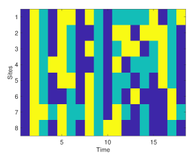
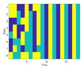
(a) PCA on a circle (b) From deterministic to stochastic (c) Synchronization
The key feature of our model is the linear dependence of the local transition probability in (1.2) on the local empirical distribution, represented by a local transition matrix. Such a linear dependence significantly reduces the number of parameters describing the local transition probability, which has a size since it assigns a -valued probability to each of the possible states of the neighborhood . Without the linear dependence, the transition probability is overly complicated for analysis and requires a significant amount of data for its estimation. In contrast, with the linear dependence, our model has only parameters instead of , significantly reducing the model complexity and the amount of data needed for inference.
The Markov chain can exhibit rich dynamics such as synchronization and ergodicity. Figure 1 illustrates two systems with and with different local transition matrices. Figure 1(b) shows a trajectory exhibiting a transition from deterministic to stochastic dynamics, and Figure 1(c) shows a trajectory exhibiting synchronization.
1.1 Main results
We first study how the local transition matrix determines important features of the global dynamics by establishing sufficient and necessary conditions on the local transition matrix for synchronization and ergodicity. When the local transition matrix is irreducible, Theorem 2.7 shows that the system will achieve a synchronization if and only if is periodic with period , and Theorem 2.10 shows that the system is exponentially ergodic if and only if is aperiodic. In short,
We then study the dependencies between the global transition probability matrix of the Markov chain and the local transition matrix. Theorem 3.2 shows that there is a 1-1 map between the global transition matrix and the local transition matrix; additionally, the invariant measure of is the marginal distribution of the invariant measure of . Theorem 3.5 shows that is Lipschitz in under the total variation norm.
In Section 4, we introduce and study the properties of least squares estimators (LSEs) for inferring the local transition matrix from various types of data. The data may consist of multiple trajectories, a long trajectory, or ensemble sequences without trajectory information. Except for the case of a long trajectory, the system can be non-ergodic. These LSEs use the marginal distributions of each vertex and are more efficient to compute than the maximal likelihood estimator, which would involve non-convex optimization. We specify identifiability conditions for these LSEs and a non-identifiability for inference using stationary distribution in Section 4.4. We show the asymptotic normality of these estimators in Theorems 4.4 and 4.10 and provide non-asymptotic bounds for their accuracy in Section 4.5. Numerical tests show that the LSE with trajectory information is more accurate than the LSE without trajectory information, while both converge at the optimal rate , with being the sample size.
1.2 Related work
Probabilistic cellular automata (PCA).
PCA are large interacting discrete stochastic dynamical systems for the modeling of a wide range of physical and societal phenomena, and we refer to [Too94, LMS90, LN18] and the reference therein for the applications. Motivated by the applications, there is consistent interest in studying the ergodicity of the systems; see, e.g., Dawson [Daw75] for a system with interacting subsystems, Follmer and Horst [FH01] for the averaged process of an interacting Markov chain with an infinite set of sites, Bérard [Bér23] for the exponential ergodicity of a 1D PCA with a local transition kernel on a three-state alphabet, and Casse [Cas23] for the ergodicity of a PCA with binary alphabet via random walks. The innovation in our model above is introducing a local transition matrix, which enables efficient estimation, while leaving the system capable of producing rich dynamics, exhibiting phenomena such as synchronization or ergodicity.
Interacting particle systems (IPSs).
IPSs are continuous-time Markov processes on certain spaces of configurations of finitely or infinitely many interacting particles. The state space can be either discrete, such as the stochastic Ising model or the voter model [Lig85, Dur07, Ald13, Gri18], or continuous in the form of stochastic differential equations [CM08, CDP18, LRW21]. The interaction rules, either short-range or long-range, are often specified by functions called interaction kernels/potentials [Lig85, CDP18] or rate functions [Ald13]. Thus, our local transition matrix can be viewed as a counterpart of these interaction kernels or rate functions.
Inference of the local transition matrix.
The inference of the local transition matrix is akin to the nonparametric estimation of the interaction kernel of interacting particle systems in [LZTM19, LMT21, DMH22, LWLM24], where inference leads to a linear inverse problem and is solved by least squares. However, the estimators in those works maximize the likelihood; here, our LSEs are different from the maximal likelihood estimator, which would lead to a constrained non-convex optimization problem, as discussed in Section 4.1.1. Also, while the identifiability conditions are specified based on the large sample limit case, in the same spirit as the coercivity condition on function spaces in [LLM+21, LL23], this study considers parametric inference, so the identifiability conditions are less restrictive.
We use the notations in Table 1 throughout the paper. We denote the entries of by with , and denote the entries of by with , where with .
| alphabet set for state values | |
| index of vertices/agents in the graph | |
| index of sample trajectories and index of time | |
| state of the Markov chain at time | |
| and | the -th vertex’s neighborhood , consisting of vertices |
| empirical distribution in at time ; -valued | |
| empirical distribution of : | |
| local transition matrix: | |
| (global) transition matrix of the Markov chain | |
| , , | Euclidean, Frobenius and operator norms |
2 Dynamical properties: synchronization and ergodicity
This section studies the dynamical properties of the process in (1.1)-(1.2) as a Markov chain with states. We fully characterize the long-time behavior of the system when the local transition matrix is irreducible. In particular, Theorem 2.7 shows that the system will achieve a synchronization if and only if is periodic with period ; Proposition 2.6 shows that the system will eventually be periodic with the same period as that of ; and Theorem 2.10 and Proposition 2.9 show that the system is exponentially ergodic if and only if is aperiodic.
To study the Markov chain, we recall the following preliminaries about a finite-state Markov chain, denoted by , which has states in and transition matrix .
-
•
Irreducible matrix. The transition matrix is called irreducible if , , such that .
-
•
Period of a matrix. The period of a state is the greatest common divisor of all such that , i.e., . When is irreducible, the period of every state is the same and is called the period of . The irreducible matrix is called aperiodic if its period is one.
-
•
Recurrence and Transience. A state is called recurrent if , where ; in other words, the chain that starts from this state returns to it in finite time with probability one. The state is called transient if . The state is called positive recurrent if .
In the following, we first present a few examples of a locally interacting Markov chain, showing that the Markov chain can have various dynamical properties. Then, we study the sufficient and necessary conditions for the system to synchronize or to be ergodic.
2.1 Examples: stochastic dynamics and synchronization
We introduce four examples: non-interacting agents, the smallest model, a system transitioning from deterministic to stochastic dynamics, and a system achieving synchronization.
Example 2.1 (Non-interacting agents)
When the agents do not interact, i.e., , they move independently according to a Markov chain with as the probability transition matrix. That is, the process is a vector of independent Markov chains with the same transition matrix .
Example 2.2 (Smallest model: )
Consider the model with . Since the neighborhood is the full network for each site, the local empirical distributions are the same for all sites, that is, we have for all states. The following table shows the local empirical distributions and the global transition matrix with a local transition matrix :
where .
Example 2.3 (From deterministic to stochastic dynamics)
The system can change from deterministic to stochastic dynamics. Let be such that for and for ; that is,
| (2.1) |
The system’s dynamics will move from deterministic to stochastic if it starts with state . Specifically, note that we have for each . Then, the value of each site moves to the next value deterministically, i.e., , for . Correspondingly, we have for each and . When , the move becomes stochastic as the last row of the local transition matrix injects the randomness. Figure 1(b) shows a typical trajectory of the system when .
Example 2.4 (Synchronization: from stochastic to deterministic dynamics)
When is a permutation matrix such that it is irreducible with period , e.g.,
| (2.2) |
the Markov chain will achieve synchronization (see Theorem 2.7), in which all sites move from one state to another with the same period as , as demonstrated in Figure 1(c) for a typical trajectory of the system when . In particular, the deterministic dynamics of the Markov chain after synchronization is as follows. Without loss of generality, suppose that it starts from the state . The local empirical distributions are for each . Then, all vertices move uniformly from one state to the next, that is, for , and then repeat periodically, as shown in the following tabular.
The corresponding local distributions are for each and .
2.2 Synchronization
We show first that the system with irreducible local transition matrix will synchronize if and only if is periodic with period .
Definition 2.5 (Synchronization)
We say the system achieves a synchronization at time if all sites move identically after , i.e., for all .
The following proposition says that if is irreducible and periodic, then the Markov chain will eventually be periodic.
Proposition 2.6
Suppose that is irreducible and periodic with period . Then
-
(i)
can be decomposed as a finite disjoint union , such that (setting ), only if and for some .
-
(ii)
For , the collection of states
is periodic with period . The collection of states is transient.
Proof. (i) This is a standard result; see, e.g.[Nor98, Theorem 1.8.4].
(ii) It follows from (i) that the states in are periodic with period . It remains to show that the states in are transient. For this, we will show that starting from for any configuration , there is some such that . Assume without loss of generality that . Since is irreducible, by part (i), there is some such that . Therefore, recalling the neighborhood , there is a positive probability that has some configuration in
i.e., the neighbors of node have the same state . Again since is irreducible, by part (i), there is some such that . So there is a positive probability that has some configuration in
i.e., the neighbors of neighbors of node have the same state . Continuing in this manner, we see that there is a positive probability for to jump after at most steps to some state in , i.e., .
Using Proposition 2.6, we have the following characterization of when synchronization occurs.
Theorem 2.7 (Synchronization)
Suppose that is irreducible. Then, the system will achieve synchronization (with period ) if and only if the period of is .
Proof. (i) First, we prove the “if” direction. Suppose the period of is . Then the decomposition of in Proposition 2.6(i) must have the form that each is a singleton. So the collection of states in Proposition 2.6(ii) is actually just
| (2.3) |
Also, by Proposition 2.6(ii), all states in are transient and will eventually jump to some state in . Therefore, the system will achieve synchronization with period .
(ii) Next, we prove the “only if” direction. Suppose that the system will achieve synchronization. Then there exists some such that, starting from , the system will jump only among the collection of states in (2.3). This implies that for some . This further implies, for each , for some , as otherwise we have for some and it contradicts the assumption that is irreducible. Finally, again by irreducibility of , we must have . Therefore, the period of is .
Remark 2.8
The arguments in the proof of Proposition 2.6 also reveal that when is reducible, it is still possible that the system will reach a synchronization. For example:
-
(i)
If has some transient states, such as , then eventually, the system will reach a synchronization and oscillate between .
-
(ii)
If has more than one communication class, such as , then eventually the system will reach a synchronization and oscillate between the configurations , or between .
2.3 Ergodicity
We show that the system with an irreducible local transition matrix is ergodic if and only if is (irreducible and) aperiodic.
Proposition 2.9
The global transition matrix is irreducible and aperiodic if and only if the stochastic matrix is irreducible and aperiodic.
Proof. (i) First, we prove the “if” direction: We will show that is irreducible and aperiodic when is irreducible and aperiodic. It suffices to show that there exists such that for all , for all .
Since is irreducible and aperiodic, there exists some such that for all and , . Fix such an . For each , implies that there exists a sequence such that . Let for . Then,
Meanwhile, noting that the neighborhood of the node includes itself, we have for any . Thus, (1.4) implies that
for any states and . Thus, for each , where is the neighborhood of the -th agent at time . Hence,
Thus, is also irreducible and aperiodic.
(ii) Next, we prove the “only if” direction. Let be irreducible and aperiodic.
Suppose is reducible. Then there exists with such that for all and , . Then for all and , , so is reducible. This leads to a contradiction, and hence must be irreducible.
Suppose is irreducible but periodic with period . Then, by Proposition 2.6(ii), is not irreducible, which is a contradiction. This completes the proof.
Theorem 2.10
Assume that the stochastic matrix is irreducible and aperiodic. Then, is irreducible, aperiodic, and hence ergodic. In particular, there exists a unique stationary distribution , all states are positive recurrent, , and there exist , and such that
| (2.4) |
Proof. By Proposition 2.9, we have that is irreducible and aperiodic. Then it remains to prove (2.4), as the rest of the statements are classic results (see, e.g., Proposition A.1 for completeness).
Since is irreducible and aperiodic, there exists some such that
Therefore for any . Hence, and
It then follows from Proposition A.2 that
For , writing , we have
This gives (2.4) with and .
The following corollary is a particular case of Theorem 2.10, with in its proof.
Corollary 2.11
Suppose for all . Then all the statements in Theorem 2.10 hold. In fact, there exists such that
3 Global and local transition matrices
We study in this section the relation between the global transition matrix and the local transition matrix , and their associated invariant measures. Throughout this section, we assume that is irreducible and aperiodic, and so is by Proposition 2.9.
3.1 Local and global transition matrices and associated invariant measures
We show that there exists a 1-1 map between the global and local transition matrices and . Furthermore, we show that is the marginal of , where and denote the unique invariant measures of and , respectively. That is, the marginal distribution of the Markov chain’s invariant measure is the same as the invariant measure of . However, the marginal distribution does not determine , as we show in Example 3.3 that there are two ’s leading to the same and different ’s; nor does the joint invariant distribution, as we show in Example 3.4 that there are two ’s leading to the same and .
Proposition 3.1 (Shift-invariance)
The transition matrix is shift invariant. Therefore, the invariant measure is shift invariant, namely, for each ,
Proof. Recall the neighborhood . Clearly, the graph is invariant under the shift of the node indices . As the transition of in (1.1) and (1.2) depends on states through the empirical distribution of neighborhood’s states, clearly the transition matrix is shift invariant. Since the invariant measure is unique, we also have shift-invariance of .
The next theorem shows that there is a 1-1 correspondence between the local and global transition matrices. In particular, is determined by entries of .
Theorem 3.2 (1-1 map between and , as the marginal of )
There is a 1-1 map between and . Furthermore, denote by the -th marginal distribution of , i.e., , . Then .
Proof. Eq.(1.4) shows that uniquely determines . It also implies that
Therefore there is a 1-1 map between and .
Next, we prove that the marginal distribution of the invariant measure of is the same as the invariant measure of . By shift-invariance in Proposition 3.1, for all . Since is the invariant measure of , we have . Applying (1.4), we can write
Note that depends on only through . Summing over , we have
By symmetry of , we have
namely .
However, one generally does not have as the product measure of . In fact, is not completely determined by . As illustrated in the following example, one can have two different ’s with the same but different ’s.
Example 3.3 (Same marginal, different invariant measures, and ’s)
Consider , and without doubling counting the other vertex.
-
(i)
If , then , , .
-
(ii)
If , then , , .
An interesting question is whether a map exists between and for the PCA. Clearly uniquely determines . The other direction is not true for a general Markov chain: there can be multiple transition matrices with the same invariant measure, as shown in Example 3.3, where two different ’s leading to the same invariant measure . Given the special structure of being determined by a local transition matrix , which has only unknowns, one may question whether the invariant measure can uniquely determine and consequently . The following example demonstrates that the answer is no.
3.2 Lipschitz dependence on the local transition matrix
We show the Lipschitz dependence of the global transition matrix and its invariant measure on the local transition matrix.
Theorem 3.5 (Lipschitz dependence on )
Given and , let be the corresponding global transition matrices and be the stationary measures. Then
where , and is the -operator norm. Also,
where .
Remark 3.6
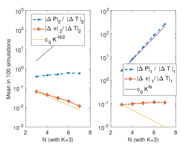
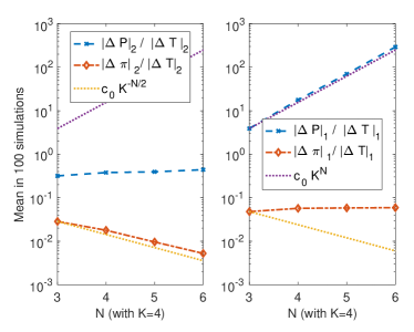
The above Lipschitz dependence on for the invariant measure is local because the constant can depend on . Numerical tests, as shown in Figure 2, suggest that the bound for is optimal, but the bound for may not.
The proof of Theorem 3.5 is based on the following lemma in [Wal20], which bounds the total variation between two invariant measures by the difference between their transition probability matrices. We refer to the general study on the perturbation of Markov chains in [Sch68, Sen88, HVdH84, CM01].
Lemma 3.7
For two finite irreducible transition matrices and with stationary distributions and ,
where .
Using this lemma and the observation that , we have the following proof for the Lipschitz estimate.
Proof of Theorem 3.5. For and , writing
we have
So, by adding and subtracting terms,
Noting that depend on only through and and are stochastic matrices, we have
Therefore
Noting that by symmetry, , we can write the last term as
Alternatively, note that
So, we also obtain
By Lemma 3.7 with the fact , we have the estimate on .
Remark 3.8 (Bounds in Frobenius norm.)
If entries of are of a similar order, then vaguely speaking one would expect
which agrees with Figure 2. But the above method only leads to a suboptimal estimate as follows:
| (3.1) |
where To see this, one can adjust the argument in the above proof and get
Since and similarly for , i.e., we have
Then, we obtain (3.1) by using symmetry to write the last term as
4 Inference of the local transition matrix
Inference is the first step in the application of the PCA model. In this section, we construct least squares estimators (LSEs) to infer the local transition matrix from various types of data. Data may consist of multiple trajectories, a long trajectory, or ensemble sequences without trajectory information as in Sections 4.1–4.3. For each of these cases, we specify identifiability conditions and prove that the estimators are asymptotically normal. Additionally, we show is non-identifiable from the stationary distribution in Section 4.4. Furthermore, we establish non-asymptotic bounds for the estimators in Section 4.5. Finally, the numerical tests in Section 4.6 demonstrate that the LSE with trajectory information is more accurate than the LSE without trajectory information, while both converge at the rate , in agreement with theory.
4.1 LSE from multiple trajectories
Consider first the inference of from data consisting of independent trajectories:
We estimate each column of through least squares, followed by a normalization. The least squares estimator minimizes the loss function
| (4.1) |
where denotes the empirical distribution :
| (4.2) |
and is the empirical distribution of the states of sample in the neighborhood of the vertex , as defined in (1.3). By solving the zero of the gradient of this loss function with respect to each , we obtain the least squares estimator from a system of normal equations with a shared normal matrix :
| (4.3) | ||||
Here, denotes the Moore-Penrose pseudo inverse of .
In practice, instead of using pseudo-inverse, we obtain by using least squares with non-negative constraints and then row-normalize the solution. The non-negative constraints help to avoid possible negative entries caused by sampling error.
Identifiability from the large sample limit.
To analyze the properties of the estimator, we first examine the inference problem in the large sample limit. Denote the large sample limit normal matrix and normal vectors by
| (4.4) | ||||
Assumption 4.1 (Identifiability condition: multi-trajectory data)
The distribution of the samples satisfies that the matrix in (4.4) is non-singular.
The assumption 4.1 holds in general, as long as the random vectors span with positive probability, as the next lemma shows.
Lemma 4.2
Proof. Recall that the covariance matrix of a random vector is singular iff there exists a vector such that a.s., which is true because iff a.s.. Applying this fact to the random vectors , we find that is singular iff there exists a fixed vector such that a.s. for all and .
When is irreducible and aperiodic, is also irreducible and aperiodic by Proposition 2.9. The number is well-defined and is finite. Then, regardless of what the initial condition is, the states visit all possible states with a positive probability, so span with a positive probability. Hence, one cannot find a such that a.s. for all .
The exceptions are extreme. For the system in either Example 2.3 or Example 2.4, the normal matrix is singular when , and is non-singular once . For the system in Example 2.3, since for each and , we can take so that for all and . In this case, is singular for any . On the other hand, if , the resulting normal matrix becomes full rank.
Asymptotic normality.
We show next that the LSE is asymptotically normal.
Theorem 4.4
Proof. For , denote
| (4.7) |
where is defined in (4.2). Note that and are independently identically distributed, and and . Thus, by the strong law of large numbers, and
for each , where the matrix in (4.6) is the covariance matrix of :
Then, by Lemma 4.5, we have . Now, the asymptotic normality of the LSE in (4.5) follows from the definition of in (4.3) and Lemma 4.3.
The following lemma is a slight extension of Slutsky’s theorem; we will use it repeatedly to study the asymptotic normality of least squares estimators. Its proof is included for completeness.
Lemma 4.5
Suppose that and as , where are two symmetric strictly positive definite matrices. Then is asymptotically normal, i.e., .
Proof. First, we have since is invertible and . Specifically, the almost sure convergence of implies that . Then, Weyl’s inequality , where denotes the minimal eigenvalue of , implies that . Thus, .
Next, combining with , we have, by Slutsky’s theorem, and . Therefore, using , we obtain .
4.1.1 Comparison with MLE and LSE using stochasticity
We discuss two other estimators, an LSE using stochasticity and the maximal likelihood estimator, and compare them with the above LSE. We show that the LSE using stochasticity is similar to the above LSE in theory, but the above LSE is computationally more stable and efficient. The maximal likelihood estimator (MLE) involves a constrained non-convex optimization, making it less effective than the LSE.
Least squares estimator using stochasticity.
We can also estimate , the first columns of , by least squares, since is a stochastic matrix. We call this estimator LSE using stochasticity.
Compared to the LSE above, this estimator has two advantages: (1) it does not need the extra normalization step, and (2) it has parameters to be estimated, removing the redundancy. However, these advantages may be offset by its computational drawbacks when is large: it solves a linear system with equations, with a normal matrix prone to be ill-conditioned, while the above LSE solves linear systems with equations, which can be done in parallel. Moreover, as shown below, the two estimators share the same identifiability condition and asymptotic behavior. Thus, the LSE is preferred in practice.
Specifically, the array is the first column of . Note that
where , and the last column follows from
Then, the loss function becomes
This loss function is quadratic, so its minimizer can be found from the zeros of its gradient. Thus, we write in vector form and write the gradient of the loss function as
where the normal matrix and vectors are, with a notation and similarly for and ,
| (4.8) | ||||
The resulting estimator is
| (4.9) |
The invertibility of the matrix is the same as the matrix in (4.3). We can write
where is a Kronecker product
Recall that the Kronecker product is invertible iff both and are invertible, and . Note that is invertible with eigenvalues and for . Hence, is nonsingular iff is nonsingular.
Maximal likelihood estimator.
We can also estimate the local transition matrix by maximizing the likelihood of data:
| (4.10) |
Note that, unlike the LSE, it is necessary to consider the optimization with respect to a stochastic matrix , because otherwise, the likelihood has no maximum.
The derivative of the loss function can be computed directly. Using the fact that , we have, for each and ,
Clearly, even with the above gradient, the uniqueness of the minimizer for the constrained optimization of a nonconvex function is relatively complicated for analysis. Thus, the asymptotic normality of the MLE is non-trivial since it relies on uniqueness. Also, while optimization algorithms can easily compute the minimizer, it remains open to provide a performance guarantee.
4.2 LSE for a single long trajectory for ergodic systems
Suppose that the system is ergodic, and we estimate the local transition matrix from data consisting of a long trajectory:
Under the ergodicity assumption, the estimation is the same as the previous case with , and we define the estimator by
| (4.11) | ||||
Here denotes the Moore-Penrose pseudoinverse of .
Similarly to the previous section, the large sample limit helps us specify the identifiability condition. Denote the large sample limit normal matrix and normal vectors by
| (4.12) | ||||
where the expectation is with respect to the stationary measure of the Markov chain.
Theorem 4.6
Proof. We omit the proof, as it is nearly identical to the case of multiple trajectories, except for applying the law of large numbers and the central limit theorem for an ergodic trajectory.
4.3 LSE from ensemble data without trajectory
Another interesting setting is when the observations are samples of for each time , but these samples may come from different trajectories. We call this setting as ensemble data without trajectory information and denote the data by
We assume that is large and study the error bounds with respect to .
We estimate by least squares that match the empirical marginal densities of each site. Recall that the marginal density of site at time is, for ,
| (4.15) | ||||
Thus, our estimator is based on empirical approximations of and :
| (4.16) | ||||
for . Note that they are determined by the empirical distributions at each time, and there is no need for sample trajectories. The sample sizes do not have to be the same at different times, as long as their minimum is large enough to make these empirical approximations reasonably accurate.
Our least squares estimator, called ensemble LSE, minimizes the discrepancy between the empirical approximations and in (4.16):
| (4.17) |
The ensemble LSE is solved by
| (4.18) | ||||||
Similar to the multi-trajectory LSE in Section 4.1, in practice, we obtain the ensemble LSE by least squares with non-negative constraints, followed by row-normalization.
This LSE can be viewed as a generalized moment estimator, since the entries in the normal matrix and normal vector are approximations of moments. We will show that the estimator is asymptotically normal under a new identifiability condition.
Identifiability in the large sample limit.
Denote the large sample limit normal matrix and normal vectors by
| (4.19) | ||||
Assumption 4.7 (Identifiability condition: ensemble data)
The distribution of the samples satisfies the fact that the matrix in (4.19) is non-singular.
Lemma 4.8
Under Assumption 4.7, .
This assumption puts constraints on both the distribution of the process and the local empirical distributions that depend on the neighborhood size of the interaction. Three factors can contribute to the identifiability: a non-symmetric initial distribution between sites, a neighborhood that can lead to varying local empirical distributions, and a process that varies in time. For example, can be full rank if has rank , which relies on a diverse initial distribution and local empirical distribution. Example 4.9 below shows an extreme case that are the same for all sites, and we rely on the distribution at different times to attain a full-rank norm matrix.
Example 4.9 (Full-network neighborhood)
The local empirical distributions are the same for all sites if the neighborhood is the entire network for each agent. For example, the model in Example 2.2 has for all states . Thus, for full-network neighborhood, we have for any . Then, we have and it is full rank only if has rank . As discussed later, the normal matrix has rank 1 when the process is stationary.
Asymptotic normality.
We show next that the ensemble LSE is asymptotically normal.
Theorem 4.10
Proof. The proof is based on the asymptotic properties of the empirical approximations of and defined in (4.16).
First, by the strong Law of Large Numbers,
as , for each . Also, by Central Limit Theorem,
| (4.21) |
for each , where the variance follows from (recall that )
Next, we study the asymptotical properties of the normal matrix and vector in (4.18). Since for each , the normal matrice must also converge a.s., i.e.,
where is defined in (4.19). Meanwhile, by Slutsky’s theorem and (4.21), we have
for each . Then, since , we have
Consequently,
with defined in (4.20).
4.4 Non-identifiability from stationary distribution
Inference from the stationary distribution is challenging since the information is limited. It is well known that a stationary distribution of a Markov chain does not determine its transition matrix, i.e., is not determined by . Similarly, the local transition matrix in our model is under-determined by the stationary distribution. Example 3.4 shows that when , there are two ’s leading to the same invariant measure. Theorem 4.11 shows that, in general, the ensemble-LSE is under-determined by the marginal invariant distribution, even though has only unknowns and the invariant measure has entries.
We start with a few basic facts when the process is stationary. By the shift-invariance in Proposition 3.1, the marginal distributions of all vertices are the same, and so are the expectation of the local empirical distributions, i.e.,
| (4.22) |
Thus, the large sample limit of the loss function in (4.17) is
| (4.23) | ||||
Theorem 4.11 (Non-identifiability from the stationary distributions)
Given only the invariant measure, the local transition matrix is under-determined, i.e., the loss function in (4.23) has multiple minimizers, either when or when with .
Proof. Note that when given only the stationary measure, the local empirical distributions can only be used via their expectations. Then, by (4.22), one can only estimate from: (1) the discrepancy between the distributions and ; and (2) the fact that by Theorem 3.2. Thus, the identifiability of is equivalent to the uniqueness of the minimizer to the loss function
| (4.24) |
Since is quadratic in , it suffices to study the invertibility of its Hessian
| (4.25) |
Here, the Hessian is with respect to and they are the same for all . The Hessian matrix has rank when ; and it has rank 1 when . Thus, there are multiple minimizers to , i.e., is under-determined, either when or when with .
The above non-identifiability is rooted in the limited information in use: only the marginal distributions are used. Loss functions other than the quadratic loss function in (4.24), such as those based on the Kullback-Leibler divergence, total variation, or Wasserstein distances between and , will also have the same issue.
4.5 Non-asymptotic bounds for the LSEs
We establish non-asymptotic bounds for the multi-trajectory LSE in (4.3) and the ensemble LSE in (4.18). Roughly speaking, for small ad , both estimators are -close to the true local transition matrix with a probability of at least when the sample size is of order , but the constant for is much larger due to the absence of trajectory information.
Theorem 4.12
Let be the true local transition matrix. For any , let and . The following non-asymptotic bounds hold.
- (a)
- (b)
The proof is based on the concentration bounds for the normal matrices and vectors in the next lemma. These bounds highlight that the trajectory-based normal matrice and vector approach their large sample limits faster than those without using trajectory information.
Lemma 4.13 (Concentration for normal matrices and vectors)
Proof. These bounds follow from applying Bernstein’s inequalities.
Part (a). First, Note that , where , defined in (4.7), is a sequence of symmetric identically distributed random matrices with mean zero and
Meanwhile, since is symmetric,
where the inequality follows from since each entry of is in . Consequently, . Applying the matrix Bernstein’s inequality (see Theorem A.4), we obtain the bound for .
Next, recall that by the definition of in (4.7), we have
with . Using the fact that and , we have and . Thus, Bernstein’s inequality (see Theorem A.3) implies
Meanwhile, note that holds true if for all . Hence,
Part (b). The normal matrix and vector in (4.18) require additional treatments since they involve products of the averages in samples. To remove these products, we use their upper bounds, which leads to a multiplicative factor in the upper bounds for the probabilities.
First, we show that
| (4.28) | ||||
Note that . Thus, we only need to prove that and . Recall that and in (4.16). Since is a probability distribution, its entries are non-negative, so . As a result,
where the last equality uses the facts that and . Similarly, the bound holds for .
Next, we show the concentration bound for . Note that
Then, using the fact that for any , , we have
where the last two inequalities follow from (4.28). Applying the Bernstein’s inequality as above, we obtain
Lastly, we consider . Using the fact that , we have
where the last two inequalities follow from (4.28). Applying Bernstein’s inequality, we obtain
This completes the proof.
Proof of Theorem 4.12. The proof is based on the Bernstein concentration inequalities for the normal matrices and the normal vectors. For Part (a), note that
where in the last inequality we have used the fact that . Hence, we have
where we denote by the following events:
Thus, . Then, if we can prove the following bounds
| (4.29) |
for , we can conclude (4.26) by noting that
In the following, we prove the three bounds in (4.29) by Bernstein’s inequalities. Note that
Thus, . Meanwhile, by Weyt’s inequality, . Hence,
which can be bounded by matrix Bernstein’s inequality. Similarly,
Thus, with , Lemma 4.13 implies,
Similarly, with , Lemma 4.13 implies,
Hence, to obtain (4.29), we set to satisfy both and , which lead to the lower bound for .
Part (b). The proof is the same as the above for Part (a).
4.6 Numerical examples
Numerical tests show that the estimators converge as sample size increases at the rate , agreeing with the theory. They also show that the sampling error may lead to estimators missing the periodic property of the local transition matrix and hence the synchronization; thus, additional techniques, such as an application of a threshold or a sparse condition, are needed to preserve the additional properties of the local transition matrix.
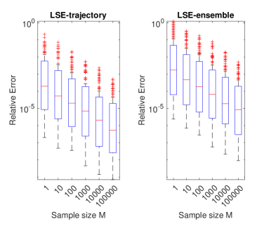
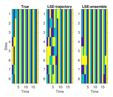
(a) Convergence in sample size (b) Synchronization Prediction
Figure 3(a) examines the convergence in sample size for the multi-trajectory LSE in Section 4.1 and the ensemble LSE in Section 4.3. That is, these estimators are obtained by first solving the normal equations by least squares with non-negative constraints and then row-normalizing the resulting solutions. Here we consider a system with . The figure shows the box plots of the relative errors of the estimators in 100 independent simulations with increasing sample size. Here we consider a randomly generated matrix , and use it to generate sample trajectories with . Then, we randomly draw samples out of them for times.
The results show that the estimators converge as sample size increases at the rate , agreeing with Theorems 4.4 and 4.10. Additionally, the multi-trajectory LSE is more accurate than the ensemble LSE; since both estimators use the same dataset each time, the better accuracy comes from the additional trajectory information.
Figure 3(b) tests the effects of the sampling error in predicting the synchronization. Here the true and estimated local transition matrices are:
The estimators are estimated using sample trajectories with . Due to the sampling error, both estimated local transition matrices are not periodic; thus, their systems will not synchronize. Figure 3(b) shows that the more accurate multi-trajectory LSE leads to numerical synchronization, while the ensemble LSE cannot maintain the synchronized motion due to the large estimation error. In practice, when the system is known to synchronize, we can apply thresholding or specification techniques to preserve the additional properties of the local transition matrix and achieve synchronization.
5 Future work
Many venues are to be explored beyond the scope of the present work.
The first venue is to study the new PCAs on general finite graphs. The graph can be more complex than the cyclic graph in this study, for example, a graph with a non-binary weight matrix for edges, or a high-dimensional lattice. The dynamical properties, such as synchronization and ergodicity, and the inference of the local transition matrix, can be studied similarly. Additionally, it is of great interest to jointly infer the local transition matrix and the weight matrix of the graph, as studied in [LWLM24] for interacting particle systems on graphs.
Another venue is to study the new PCAs on infinite graphs. Concerning the dynamical properties, one can study the ergodicity and the critical phenomena by extending the results in [Too94, LMS90, Cas23, Bér23, FH01]. Concerning the inference of the local transition matrix, one may consider the asymptotic and non-asymptotic properties of the estimator when the data is a single trajectory with , for which [DMH23] has established similar results for interacting particle systems and [BZ24] considered this problem for graphon particle systems; see, e.g., [BCW23]. An interesting parameter to estimate in a similar context would be the size of each neighborhood.
Appendix A Preliminaries on Markov chain and concentration inequalities
A.1 Properties of Markov chains
Suppose is a finite-state Markov chain with transition matrix . We recall the following general results for Markov chains.
Proposition A.1
-
•
There is a stationary distribution . (because , where denotes the transition matrix, is not of full rank)
-
•
All states are positive recurrent; see [Dur19, Theorem 1.30].
-
•
Suppose is aperiodic. Then ; see [Dur19, Theorem 1.19].
-
•
; see [Dur19, Theorem 1.23].
-
•
Suppose . Then ; see [Dur19, Theorem 1.22].
Regarding the exponential convergence to the stationary distribution, we have the following result taken from [Kul15, Theorem 1.3].
Proposition A.2
Suppose there is some such that
| (A.1) |
Then . In addition,
A.2 Concentration inequalities
Theorem A.3 (Bernstein’s Inequality)
(see e.g., [Ver18, Theorem 2.8.4]) Let be independent zero-mean random variables. Suppose that almost surely for all . Then for all positive , In particular, when are iid., we have .
Theorem A.4 (Matrix Bernstein’s inequality)
Acknowledgement
This work is supported by the following grants: NSF-1913243, NSF-2106556 FA9550-21-1-0317, and FA9550-23-1-0445.
References
- [Ald13] David Aldous. Interacting particle systems as stochastic social dynamics. Bernoulli, 19(4):1122–1149, 2013.
- [BCW23] Erhan Bayraktar, Suman Chakraborty, and Ruoyu Wu. Graphon mean field systems. Ann. Appl. Probab., 33(5):3587–3619, 2023.
- [Bér23] Jean Bérard. Coupling from the past for exponentially ergodic one-dimensional probabilistic cellular automata. Electronic Journal of Probability, 28:1–17, 2023.
- [BZ24] Erhan Bayraktar and Hongyi Zhou. Non-parametric estimates for graphon mean-field particle systems, 2024.
- [Cas23] Jérôme Casse. Ergodicity of some probabilistic cellular automata with binary alphabet via random walks. Electronic Journal of Probability, 28:1–17, 2023.
- [CDP18] Patrick Cattiaux, Fanny Delebecque, and Laure Pédèches. Stochastic Cucker–Smale models: Old and new. Ann. Appl. Probab., 28(5):3239–3286, 2018.
- [CM01] Grace E Cho and Carl D Meyer. Comparison of perturbation bounds for the stationary distribution of a Markov chain. Linear Algebra and its Applications, 335(1-3):137–150, 2001.
- [CM08] Felipe Cucker and Ernesto Mordecki. Flocking in noisy environments. Journal de Mathématiques Pures et Appliquées, 89(3):278–296, 2008.
- [Daw75] DA Dawson. Information flow in graphs. Stochastic Processes and their applications, 3(2):137–151, 1975.
- [DMH22] Laetitia Della Maestra and Marc Hoffmann. Nonparametric estimation for interacting particle systems: McKean-Vlasov models. Probability Theory and Related Fields, pages 1–63, 2022.
- [DMH23] Laetitia Della Maestra and Marc Hoffmann. The lan property for mckean–vlasov models in a mean-field regime. Stochastic Processes and their Applications, 155:109–146, 2023.
- [Dur07] Richard Durrett. Random graph dynamics, volume 200. Cambridge University Press, 2007.
- [Dur19] Rick Durrett. Probability: theory and examples, volume 49. Cambridge University Press, 2019.
- [FH01] Hans Föllmer and Ulrich Horst. Convergence of locally and globally interacting Markov chains. Stochastic Processes and Their Applications, 96(1):99–121, 2001.
- [Gri18] Geoffrey Grimmett. Probability on graphs: random processes on graphs and lattices, volume 8. Cambridge University Press, 2018.
- [HVdH84] Moshe Haviv and Ludo Van der Heyden. Perturbation bounds for the stationary probabilities of a finite Markov chain. Advances in Applied Probability, 16(4):804–818, 1984.
- [Kul15] Alexei Kulik. Introduction to Ergodic rates for Markov chains and processes: with applications to limit theorems, volume 2. Universitätsverlag Potsdam, 2015.
- [Lig85] Thomas Milton Liggett. Interacting particle systems, volume 2. Springer, 1985.
- [LL23] Zhongyang Li and Fei Lu. On the coercivity condition in the learning of interacting particle systems. Stochastics and Dynamics, page 2340003, 2023.
- [LLM+21] Zhongyang Li, Fei Lu, Mauro Maggioni, Sui Tang, and Cheng Zhang. On the identifiability of interaction functions in systems of interacting particles. Stochastic Processes and their Applications, 132:135–163, 2021.
- [LMS90] Joel L Lebowitz, Christian Maes, and Eugene R Speer. Statistical mechanics of probabilistic cellular automata. Journal of statistical physics, 59:117–170, 1990.
- [LMT21] Fei Lu, Mauro Maggioni, and Sui Tang. Learning interaction kernels in stochastic systems of interacting particles from multiple trajectories. Foundations of Computational Mathematics, pages 1–55, 2021.
- [LN18] Pierre-Yves Louis and Francesca R Nardi. Probabilistic cellular automata. Emergence, Complexity, Computation, 27, 2018.
- [LRW21] Daniel Lacker, Kavita Ramanan, and Ruoyu Wu. Locally interacting diffusions as Markov random fields on path space. Stochastic Processes and their Applications, 140:81–114, 2021.
- [LWLM24] Quanjun Lang, Xiong Wang, Fei Lu, and Mauro Maggioni. Interacting particle systems on networks: joint inference of the network and the interaction kernel. arXiv preprint arXiv:2402.08412, 2024.
- [LZTM19] Fei Lu, Ming Zhong, Sui Tang, and Mauro Maggioni. Nonparametric inference of interaction laws in systems of agents from trajectory data. Proc. Natl. Acad. Sci. USA, 116(29):14424–14433, 2019.
- [Nor98] James R Norris. Markov chains, volume 2. Cambridge University Press, 1998.
- [Sch68] Paul J Schweitzer. Perturbation theory and finite Markov chains. Journal of Applied Probability, 5(2):401–413, 1968.
- [Sen88] Eugene Seneta. Perturbation of the stationary distribution measured by ergodicity coefficients. Advances in Applied Probability, 20(1):228–230, 1988.
- [Too94] Andrei Toom. On critical phenomena in interacting growth systems. part i: General. Journal of statistical physics, 74:91–109, 1994.
- [Tro15] Joel A. Tropp. An introduction to matrix concentration inequalities. Foundations and Trends in Machine Learning, 8(1-2):1–230, 2015.
- [Ver18] Roman Vershynin. High-dimensional probability: An introduction with applications in data science, volume 47. Cambridge University Press, 2018.
- [Wal20] Neil Walton. Pertubation of Markov chains. https://appliedprobability.blog/2020/08/07/perturbation-of-markov-matrices/, 2020.