Optimal Sampling for Uncertainty-of-Information Minimization in a Remote Monitoring System
Abstract
In this paper, we study a remote monitoring system where a receiver observes a remote binary Markov source and decides whether to sample and transmit the state through a randomly delayed channel. We adopt uncertainty of information (UoI), defined as the entropy conditional on past observations at the receiver, as a metric of value of information, in contrast to the traditional state-agnostic nonlinear age of information (AoI) penalty functions. To address the limitations of prior UoI research that assumes one-time-slot delays, we extend our analysis to scenarios with random delays. We model the problem as a partially observable Markov decision process (POMDP) problem and simplify it to a semi-Markov decision process (SMDP) by introducing the belief state. We propose two algorithms: A globally optimal bisection relative value iteration (bisec-RVI) algorithm and a computationally efficient sub-optimal index-based threshold algorithm to solve the long-term average UoI minimization problem. Numerical simulations demonstrate that our sampling policies surpass traditional zero wait and AoI-optimal policies, particularly under conditions of large delay, with the sub-optimal policy nearly matching the performance of the optimal one.
Index Terms:
Remote monitoring, uncertainty of information, age of information, Markov decision processI Introduction
To evaluate the information freshness, age of information (AoI) has been proposed in [1], [2], and has attracted extensive research attention in remote monitoring, industrial automation, and internet-of-things (IoT) applications [3, 4, 5, 6, 7, 8, 9, 10, 11]. Traditionally, AoI is known to be state-agnostic [12, 13, 14], i.e., focusing solely on the timeliness of information without accounting for the dynamics and the semantics of the source. Today, some variants of AoI have been proposed in [15, 16, 17, 18, 19, 20, 21, 22, 23, 24] to address the state-agnostic limitation. The researchers successfully derive their metrics of interest, such as the mutual information and the mean square error between the source and the latest receives message, as non-linear penalty functions of AoI. In this way, the problem of minimizing mutual information, or mean square error, can be transformed into a problem of minimizing non-linearly penalized AoI.
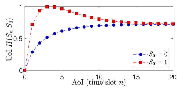
Uncertainty of information (UoI) is a new metric that addresses the state-agnostic limitation of AoI [25]. Defined as the entropy conditional on past observations at the receiver, UoI quantifies the receiver’s uncertainty about the latest state of the source based on previously received, potentially outdated observations. Unlike AoI, UoI integrates both the age and the historical observations, making it a state-aware metric. For example, consider a binary discrete-time Markov process with state transition probabilities and . As illustrated in Fig. 1, UoI’s dependence on AoI varies with the latest received state , exhibiting a non-monotonic relationship. This phenomenon introduces new challenges in designing UoI-optimal sampling policies.
In [25] and [26], the UoI-optimal sampling and scheduling policy has been investigated in the one-time-slot system. In [25], a Whittle index-based multi-source scheduling policy for binary Markov process is derived. Then an index policy for general finite-state Markov processes under unreliable channels are further extended in [26]. Both of the studies idealize the transmission delay as one time slot. However, random and large delays are common in communication networks due to network loading, routing, and retransmission[27]. Under random delay, UoI-optimal sampling process is no longer a typical Markov decision process (MDP), which brings about new challange. This prompts us to formulate a new problem for UoI-minimization under random delay.
Up to this point, considerable research efforts have been devoted to optimizing metrics related to AoI in the presence of delays [28, 29, 30, 31, 32, 33]. Authors proposes a new “selection-from-buffer” model for sending the features aimed at minimizing the general functions of AoI (monotonic or non-monotonic) with random transmission delay in [30]. As an extension to [30], authors minimizes the general functions of AoI through a channel with highly variable two-way random delay in [32]. And in [33], an optimal sampling policy is designed to minimize the average AoI when the statistics of delay are unknown. However, all of these AoI-related functions to be minimized are state-agnostic, distinct to minimization of UoI, which is a state-aware metric.
To sum up, our motivation is twofold: () The optimization of UoI under random delay still remains largely unexplored. () The UoI-minimization problem is distinct from other AoI-related optimization under random delay. In this paper, we study a remote monitoring system where a receiver observes a remote binary Markov source and decides whether to sample the source’s state over a randomly delayed channel. Our goal is to solve a UoI-minimization problem under random delay. We model the problem as a partially observed Markov decision process (POMDP), and simplify it into a semi-Markov decision process (SMDP) by introducing belief state. Specifically, the contributions of this paper are as follows:
-
•
We formulate a new problem to minimize the average UoI under random delay.
-
•
We propose an optimal policy for this work. An optimal sampling policy is provided by applying a two layered bisection relative value iteration (bisec-RVI) algorithm.
-
•
We develop a sub-optimal policy for this work. A sub-optimal index policy with computation efficiency is proposed based on the special properties of belief state.
Numerical simulations illustrate that our proposed sampling policies outperform traditional Zero wait and AoI-optimal policies. And the performance of the sub-optimal policy nearly match that of the optimal policy, especially under large delay.
II System Model and Problem Formulation
II-A System Model
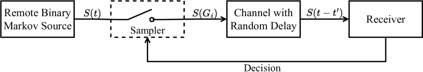
We consider a discrete-time remote monitoring system in Fig. 2, where the states of a remote binary Markov source are delivered through a channel to a receiver. Based on the history observation of the source’s state, the receiver decides whether to sample the current state or not, and transmits the decision to the sampler. The remote source is a discrete-time binary Markov process with a state at time denoted by . We assume that the one-step transition matrix of the Markov process is known to the receiver, given by
| (1) |
where , 111Without loss of generality, we assume that . And when , UoI is constant that can not be changed by any sampling policy. For a similar reason, we also assume that and .. Consequently, the -step transition matrix of this Markov process is [34, Appendix A]
| (2) |
where , , .
The -th state information sent over the channel is sampled and transmitted in time slot , and is delivered at the receiver at time slot , where is the independent and identically distributed (i.i.d) random transmission delay of the -th state information, satisfying . We assume that the sampler receives delay-free decision commands from the receiver 222A remote monitoring system with two-way random delay can be extended based on this work. , such that the receiver sends the decision and the sampler receives the decision at time slot . Let represent the waiting time for sending the -th packet after the ()-th packet is received by the receiver.
II-B Problem Formmulation
The UoI is a metric proposed in [25] to measure the uncertainty of the source at the receiver side given the history observations, given by
| (3) |
where are the history observations at the receiver side up to time slot , and is the time stamp of the most recently received update. Leveraging the Markov property of , we have
| (4) | ||||
From the definition of , we can rewrite as a piecewise function:
| (5) | |||
For short-hand notations, we introduce as the entropy of a binary information. With (2) in hand, (5) can be rewritten as
| (6) |
where for is what exactly AoI indicates. As a result, UoI is an observation-based non-monotonic function of AoI.
A sampling policy is a sequence , which is time stamps of sampling times for each packet. Alternatively, the sampling policy can also be expressed as , which is the sequence of waiting times for each packet. (see B for a detailed explanation.) Our goal is to find both an optimal sampling policy that minimizes the time-average expected sum-UoI:
| (7) |
This is a new problem different from previous studies focused on optimizing cost functions of AoI with random delay. The uniqueness resides in the fact that UoI is not only dependent on the age of the latest observation (i.e. ), but also customized by the latest observation , as shown in (LABEL:eq2-6). Compared to UoI, the current functions of AoI used as metrics to design sampling policy under random delay, as we know, have nothing to do with the contents of the transmission information and remains invariant [30, 31, 32].
III Optimal Sampling policy
In this section, we propose an optimal sampling policy by using bisec-RVI algorithm to minimize the long-term average expected sum-UoI.
III-A Belief State
In our system model, the receiver is tasked with determining sampling actions based on delayed and imperfect observations to minimize the time-average UoI. This problem is commonly modeled as a POMDP. A fundamental approach in solving partially observable Markov decision processes (POMDPs) involves transforming them into Markov Decision Processes (MDPs) by utilizing a concept known as belief state. In this subsection, we explore the belief state in our context, which is as the probability of given the observations , given by
| (8) |
Similar to the process to obtain (LABEL:eq2-6), we can prove that for , , can be expressed by
| (9) |
The evolution of the belief state is given in the following lemma:
Lemma 1.
Given , can be explicitly calculated by
| (10) |
where , . For short-hand notations, we leverage to denote the right-hand side of (10).
Proof.
Please refer to A.∎
Corollary 1.
The equilibrium belief state of is
| (11) |
Proof.
Since , we have that , and thus we obtain the limit. ∎
III-B An Optimal Sampling Policy
We present an optimal policy for (13) as follows:
Theorem 1.
If ’s are with a finite mean , given , then is an optimal solution to (13), which satisfies the following optimality equation:
| (14) | ||||
| (15) |
where
| (16) |
| (17) | ||||
for all , .
Proof sketch.
The problem (13) can be cast as an infinite-horizon average cost SMDP [34, Chapter 11]. Recall that as the waiting time for sending the -th packet after the -th packet is received by the receiver. Given , the Bellman optimality equation of the average cost problem is
| (18) | ||||
for all , , where is the relative value function associated with the average cost problem (13).
We assume that ’s are random variables with limited values, thus the states of are finite and countable. The equation (18) can be converted to (14) and (15). This inversion can be interpreted as a transformation from the SMDP to an equivalent MDP [34, Chapter 11]. Please refer to Appendix B for details of the proof. ∎
Applying Dinkelbach’s method for nonlinear fractional programming as shown in [35] and [36, lemma 2], we get two assertions: () if and only if . () is the unique root of . Consequently, we can find the value of by finding the root of as shown in Algorithm 1, which is a two-layered Bisec-RVI algorithm. Bisection search method is applied to the outer layer to get a fixed for every step and finally get the optimal value . In the inner layer, as the value of has been fixed by the outer layer, we only need to use RVI to find convergent . The RVI algorithm here is the same as it in MDP. The details about RVI algorithm have been neglected since it has been a mature technique to solve an infinite-horizon MDP [34, Section 8.5.5]. Similar algorithms are proposed in [23, 37] and [38] to achieve age-optimal or mean square error (MSE)-optimal sampling.
IV Sub-optimal Index-based Policy
The optimal policy for (13) uses bisec-RVI algrithm, which requires repeatedly executing the RVI algorithm in the inner layer until the value to be found converges, resulting in high computing complexity.
In this section, we explore a sub-optimal but computation-efficient index-based policy in the sequel. We assume that the transmission process spends a long time, i.e., the value of , is large enough. The large transmission delay may be due to long distance, time-varying channel conditions, too many packets in the channel and so on. According to (11), we can conclude that the transition probability from receiving time to () is
| (19) |
As the state transition probabilities are constant, the second and third terms of the right-hand-side of (18) are irrelevant to the waiting time, making the Bellman optimality equation easier to solve. Along this line, we can finally get an index-based sampling policy.
We depict the details of the problem as follows. On the basis of the assumption, we consider a sampling policy and try to optimize the following problem:
| (20) |
After that, we present an index-based sampling policy for the problem. We introduce an index function as
| (21) |
where , .
Theorem 2.
If ’s are with a finite mean , then is an optimal solution to (15), where
| (22) |
and is the unique root of
| (23) |
where is the receiving time of the -th state information submitted to the channel, and is the belief state at time slot . Moreover, is exactly the optimum value of (15), i.e., .
Proof sketch.
The problem (20) can be cast as an infinite-horizon average cost SMDP. Given , the Bellman optimality equation of the average cost problem is
| (24) | ||||
for all , , where is the relative value function associated with the average cost problem (20). Theorem 2 is proven by directly solving (24). The details are provided in C. ∎
Theorem 2 signifies that the optimal solution to (20) is an index-based threshold policy, where the index function depends on the belief state. Specifically, the state of the source is submitted in time slot if two conditions are satisfied: () The channel is idle in time slot , () the index exceeds a threshold (i.e., ). where the threshold is exactly the optimum value of (20).
For notational simplicity, we rewrite (13) as
| (25) |
where and . Then a low-complexity algorithm for finding the optimal objective value is provided as algorithm 2.
Compared the relative value function (24) with (18), the core difference is that the state transition probabilities in (24) are irrelevant to the waiting time, which leads to an index policy for problem (20). According to the convergence of to in (11), we induce that if is large enough, the index policy is the optimal policy for (13), i.e., .
V Numerical Results
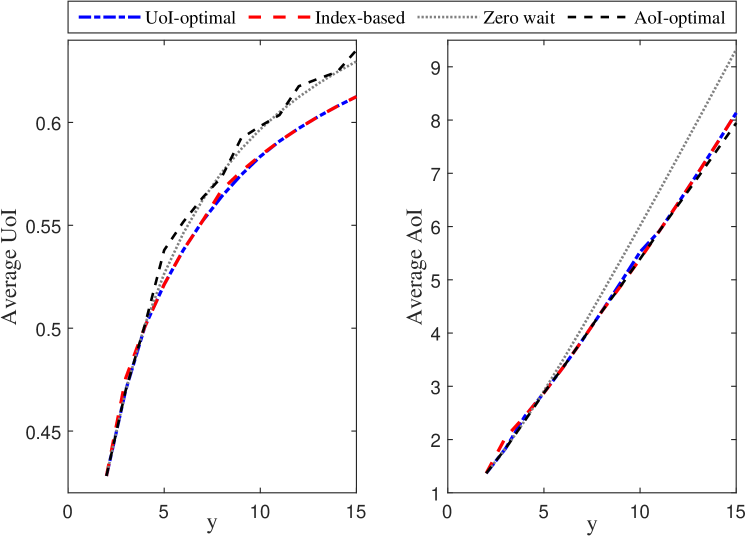
This section presents numerical results that demonstrate the performance of the index-based threshold policy. As shown in [25, Fig. 3], the -step belief state evolutions with and with are quite different, so we operate both of them in the simulations. First, we evaluate the following four sampling policies:
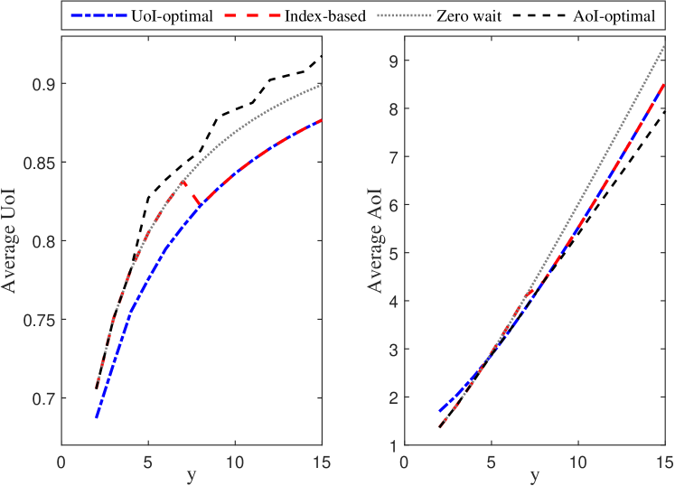
Fig. 3 shows the four policies comparison in terms of average UoI and average AoI, when the binary Markov source evaluates with the probability . The left panel shows that the average UoI obtained by the index policy is very close to the UoI-optimal one, compared to which Zero wait and AoI-optimal policy performs not well as increases. However, the right panel reveals that AoI-optimal policy consistently achieves the lowest AoI. This implies that the desired goal the receiver tends to achieve leads to different result.
In Fig. 4, we compare the four policies performance for the evaluated case that . The left panel shows a similar trend to the left panel of Fig. 3, except for the sub-optimal index-based policy. A watershed phenomenon occurs for the index-based policy: When , the index-based policy provides the same sampling strategy as zero wait policy, which performs worse than optimal policy; when , the index-based policy performs as well as the optimal policy. The reason for this phenomenon is that the index-based threshold policy is sub-optimal, deciding whether to sample or not by the comparison between the index and the constant value . Therefore, this sub-optimal policy can not always take future circumstances into account if the value of is small, thus ignores the oscillation of when . The index is always less than if , causing the zero wait policy. Otherwise, if , the index outweighs so the policy is optimal. The right panel demonstrates the lowest AoI is obtained by AoI-optimal policy as well.
The performance gains of UoI-optimal and index-based policies are close to the best average AoI, making them better choices when the system aims to optimize both AoI and UoI simultaneously. Moreover, Both of the pictures show that when is large enough, the result of index policy is the same as that of the UoI-optimal policy, consistent with the theoretical induction we proposed before. But for what exact value is meaning "large enough", is still an open issue.
VI Conclusion
In this paper, we have used UoI as a state-aware metric to estimate the value of information in a remote monitoring system. First we have put forward an optimal policy to minimize the time-average expected sum-UoI by two-layered bisec-RVI algorithm. Based on the properties of belief state, we have further provided a sub-optimal index-based sampling policy owning lower computing complexity than the optimal one. The good performance of the sampling policies have been demonstrated by numerical simulations. Both of the proposed sampling policies outperform zero wait policy and AoI-optimal policy. Moreover, the performance of the sub-optimal policy approaches to that of the optimal policy, particularly under large delay. In the future work, it may be worthwhile to investigate the specific value of that leads to the sub-optimal policy being identical to the optimal policy.
References
- [1] S. K. Kaul, R. D. Yates, and M. Gruteser, “Real-time status: How often should one update?” in Proc. IEEE INFOCOM, Mar. 2012, pp. 2731–2735.
- [2] S. K. Kaul, M. Gruteser, V. Rai, and J. B. Kenney, “Minimizing age of information in vehicular networks,” in Proc. 8th Annu. IEEE Commun. Soc. Conf. Sensor, Mesh Ad Hoc Commun. and Netw., Jun. 2011, pp. 350–358.
- [3] R. D. Yates, Y. Sun, D. R. Brown, S. K. Kaul, E. Modiano, and S. Ulukus, “Age of information: An introduction and survey,” IEEE J. Sel. Areas Commun., vol. 39, no. 5, pp. 1183–1210, Sep. 2021.
- [4] O. Dogan and N. Akar, “The multi-source probabilistically preemptive M/PH/1/1 queue with packet errors,” IEEE Trans. Commun., vol. 69, no. 11, pp. 7297–7308, Dec. 2021.
- [5] S. Wu, Z. Deng, A. Li, J. Jiao, N. Zhang, and Q. Zhang, “Minimizing age-of-information in HARQ-CC aided NOMA systems,” IEEE Trans. Wirel. Commun., vol. 22, no. 2, pp. 1072–1086, Feb. 2023.
- [6] H. Pan, T. Chan, V. C. M. Leung, and J. Li, “Age of information in physical-layer network coding enabled two-way relay networks,” IEEE Trans. Mob. Comput., vol. 22, no. 8, pp. 4485–4499, Jul. 2023.
- [7] M. Xie, Q. Wang, J. Gong, and X. Ma, “Age and energy analysis for LDPC coded status update with and without ARQ,” IEEE Internet Things J., vol. 7, no. 10, pp. 10 388–10 400, Oct. 2020.
- [8] S. Meng, S. Wu, A. Li, J. Jiao, N. Zhang, and Q. Zhang, “Analysis and optimization of the HARQ-based spinal coded timely status update system,” IEEE Trans. Commun., vol. 70, no. 10, pp. 6425–6440, Nov. 2022.
- [9] Y. Wang, S. Wu, J. Jiao, W. Wu, Y. Wang, and Q. Zhang, “Age-optimal transmission policy with HARQ for freshness-critical vehicular status updates in space-air-ground-integrated networks,” IEEE Internet Things J., vol. 9, no. 8, pp. 5719–5729, Aug. 2022.
- [10] Y. Long, W. Zhang, S. Gong, X. Luo, and D. Niyato, “AoI-aware scheduling and trajectory optimization for multi-UAV-assisted wireless networks,” in IEEE GLOBECOM, Jan. 2022, pp. 2163–2168.
- [11] H. Feng, J. Wang, Z. Fang, J. Chen, and D. Do, “Evaluating aoi-centric HARQ protocols for UAV networks,” IEEE Trans. Commun., vol. 72, no. 1, pp. 288–301, Feb. 2024.
- [12] A. Maatouk, S. Kriouile, M. Assaad, and A. Ephremides, “The age of incorrect information: A new performance metric for status updates,” IEEE/ACM Trans. Netw., vol. 28, no. 5, pp. 2215–2228, Nov. 2020.
- [13] M. Kountouris and N. Pappas, “Semantics-empowered communication for networked intelligent systems,” IEEE Commun. Mag., vol. 59, no. 6, pp. 96–102, Jul. 2021.
- [14] A. Li, S. Wu, S. Meng, R. Lu, S. Sun, and Q. Zhang, “Towards goal-oriented semantic communications: New metrics, open challenges, and future research directions,” IEEE Wirel. Commun. to appear, 2024. [Online]. Available: https://doi.org/10.48550/arXiv.2304.00848
- [15] M. Salimnejad, M. Kountouris, and N. Pappas, “Real-time reconstruction of Markov sources and remote actuation over wireless channels,” IEEE Trans. Commun., Jan. 2024.
- [16] Y. Sun and B. Cyr, “Information aging through queues: A mutual information perspective,” in Proc. IEEE SPAWC Workshop, 2018.
- [17] M. Salimnejad, M. Kountouris, and N. Pappas, “State-aware real-time tracking and remote reconstruction of a Markov source,” J. Commun. Networks, vol. 25, no. 5, pp. 657–669, Oct. 2023.
- [18] Z. Wang, M. Badiu, and J. P. Coon, “A framework for characterizing the value of information in hidden markov models,” IEEE Trans. Inf. Theory, vol. 68, no. 8, pp. 5203–5216, Jul. 2022.
- [19] Y. Sun and B. Cyr, “Sampling for data freshness optimization: Non-linear age functions,” J. Commun. Networks, vol. 21, no. 3, pp. 204–219, 2019.
- [20] J. P. Champati, M. Skoglund, M. Jansson, and J. Gross, “Detecting state transitions of a markov source: Sampling frequency and age trade-off,” IEEE Trans. Commun., vol. 70, no. 5, pp. 3081–3095, Jun. 2022.
- [21] V. Tripathi and E. H. Modiano, “A whittle index approach to minimizing functions of age of information,” in Proc. 57th Annu. Allerton Conf. on Commun., Control, and Comput., (Allerton), 2019, pp. 1160–1167.
- [22] M. Klügel, M. H. Mamduhi, S. Hirche, and W. Kellerer, “AoI-penalty minimization for networked control systems with packet loss,” in Proc. IEEE Conf. on Comput. Commun. Workshops, 2019, pp. 189–196.
- [23] Y. Sun, E. Uysal-Biyikoglu, R. D. Yates, C. E. Koksal, and N. B. Shroff, “Update or wait: How to keep your data fresh,” IEEE Trans. Inf. Theory, vol. 63, no. 11, pp. 7492–7508, Mar. 2017.
- [24] N. Pappas and M. Kountouris, “Goal-oriented communication for real-time tracking in autonomous systems,” in Proc. IEEE Inter. Conf. on Autom. Syst., 2021, pp. 1–5.
- [25] G. Chen, S. C. Liew, and Y. Shao, “Uncertainty-of-information scheduling: A restless multi-armed bandit framework,” IEEE Trans. Inf. Theory, vol. 68, no. 9, pp. 6151–6173, Srp. 2022.
- [26] G. Chen and S. C. Liew, “An index policy for minimizing the uncertainty-of-information of markov sources,” IEEE Trans. Inf. Theory, vol. 70, no. 1, pp. 698–721, Jan. 2023.
- [27] W. Yao, L. Jiang, Q. H. Wu, J. Y. Wen, and S. J. Cheng, “Delay-dependent stability analysis of the power system with a wide-area damping controller embedded,” IEEE Trans. Power Syst., vol. 26, no. 1, pp. 233–240, Dec. 2011.
- [28] Y. Sun, Y. Polyanskiy, and E. Uysal, “Sampling of the Wiener process for remote estimation over a channel with random delay,” IEEE Trans. Inf. Theory, vol. 66, no. 2, pp. 1118–1135, 2020.
- [29] C. Tsai and C. Wang, “Unifying AoI minimization and remote estimation - optimal sensor/controller coordination with random two-way delay,” IEEE/ACM Trans. Netw., vol. 30, no. 1, pp. 229–242, Mar. 2022.
- [30] M. K. C. Shisher and Y. Sun, “How does data freshness affect real-time supervised learning?” in Proc. ACM MobiHoc, 2022, pp. 31–40.
- [31] M. Moltafet, M. Leinonen, M. Codreanu, and R. D. Yates, “Status update control and analysis under two-way delay,” IEEE/ACM Trans. Netw., vol. 31, no. 6, pp. 2918–2933, Jan. 2023.
- [32] C. Ari, M. K. C. Shisher, E. Uysal, and Y. Sun, “Goal-oriented communications for remote inference under two-way delay with memory,” arXiv, 2023. [Online]. Available: https://doi.org/10.48550/arXiv.2311.11143
- [33] H. Tang, Y. Chen, J. Wang, P. Yang, and L. Tassiulas, “Age optimal sampling under unknown delay statistics,” IEEE Trans. Inf. Theory, vol. 69, no. 2, pp. 1295–1314, Feb. 2023.
- [34] M. L. Puterman, Markov Decision Processes: Discrete Stochastic Dynamic Programming. Hoboken, NJ, USA: Wiley, 2005.
- [35] W. Dinkelbach, “On nonlinear fractional programming,” Manag. Sci, vol. 13, no. 7, pp. 492–498, 1967.
- [36] Y. Sun, Y. Polyanskiy, and E. Uysal, “Sampling of the Wiener process for remote estimation over a channel with random delay,” IEEE Trans. Inf. Theory, vol. 66, no. 2, pp. 1118–1135, 2020.
- [37] Y. Sun and B. Cyr, “Sampling for data freshness optimization: Non-linear age functions,” J. Commun. Networks, vol. 21, no. 3, pp. 204–219, Sep. 2019.
- [38] H. Tang, Y. Sun, and L. Tassiulas, “Sampling of the Wiener process for remote estimation over a channel with unknown delay statistics,” in Proc. MobiHoc, 2022, p. 51–60.
- [39] D. Bertsekas, Dynamic programming and optimal control: Volume I. Nashua, NH, USA: Athena Scientific, 2012.
- [40] V. Krishnamurthy, Partially observed Markov decision processes. Cambridge, U.K.: Cambridge University Press & Assessment, 2016.
- [41] P. Haas, Stochastic petri nets: Modelling, stability, simulation. Berlin, Germany: Springer Science & Business Media, 2006.
Appendix A The Proof of lemma 1
Here is the detailed process for the evaluation of the belief state. With the transition matrix given in (2), the evolution of the belief state can be written as
| (26) | ||||
The prood is completed.
Appendix B The proof of Theorem 1
The sampling problem (13) is an infinite-horizon average cost semi-Markov decision process (SMDP) [39, Chapter 5.6] [34, Chapter 11]. In accordance with the description provided in [39, Chapter 5.6], we elaborate on the various components of this problem blow:
-
•
Decision Time: Because the control commands from the receiver are promptly delivered to the sampler without delay, each -th receiving time also serves as a decision time of the problem (13), where is the submission time of the -th packet, taking time slots to be delivered to the receiver.
-
•
State: The belief state . At time slot , the state of the system is the belief state .
-
•
Action: is the waiting time for submitting the -th packet after the -th packet is received. We consider , and for each . Consequently, given , the sequence is uniquely determined by . Therefore, is a valid representation to a policy in .
-
•
State Transitions: The state evolves as follows:
(27) where . From (10) we can get the transition probability is
(28) (29) -
•
Expected Transition Time: The expected time difference between the decision times and is
-
•
Expected Transition Cost: The expected cumulative cost incurred during the interval between the decision times and can be calculated as
(30)
We can use dynamic programming [39] to solve the average-cost SMDP (13). If , then the optimal decision for the -th packet satisfies the following Bellman optimality equation
| (31) | ||||
where is the relative value function associated with the average cost problem (20).
According to [34, Chapter 11], we can transform the SMDP into an equivalent Markov decision process (MDP). First, we rewrite the objective function in problem (13) by taking the limit superior of the ratio of the total expected transition cost to the -th decision epoch () to the total expected transition time as follows:
| (32) | ||||
where . As a result, (13) can be expressed as
| (33) |
To solve the problem (33), we consider the following problem with a parameter :
| (34) |
For each constant , the problem (B) can be cast as a MDP problem with components below:
-
•
State: The state of the MDP is the belief state at time for .
-
•
Action: The waiting time for .
-
•
Transition Probability: The transition probability is given by
(35) (36) -
•
Cost Function: The cost function is defined by
(37) where .
As the state space is finite and the optimality of the MDP can be achieved by a unichain policy, the optimal policy is determined by the optimality equation as follows:
| (38) | ||||
where is the average cost achieved by the optimal policy, is the value function.
This infinite-horizon MDP problem can be solved by using relative value iteration (RVI) [40, Section 6.5.2]. To adapt to the RVI algorithm, we rewrite the optimality equation (38) in the following form that is anchored at state . Define , so . Then (38) can be rewritten relative to state as
| (39) |
| (40) |
where
| (41) | ||||
It is worthwhile to note that we assume that the state belongs to the state space here, if not the anchor point can be changed to other state in the state space.
Next, we proof that the optimal policy for problem (13) and the optimal policy for problem in (B) are identical, i.e., . By similarly applying Dinkelbach’s method for nonlinear fractional programming as in [35] and [36, lemma 2], we get two assertions in the following lemma:
Lemma 2.
There are two assertions that hold true as follows:
-
1.
if and only if .
-
2.
is the unique root of .
Proof.
Please see Appendix D for detaied proof. ∎
Consequently, we have . And there exists an optimal policy satisfying that
| (42) | ||||
which implies that for policy ,
| (43) |
Because (43) is equal to (33), the policy is also the optimal policy of problem (13), i.e., .
Therefore, the optimality equation of the SMDP problem (31) can be converted into the optimality equation of the MDP problem in (B), given by
| (44) | ||||
| (45) |
where
| (46) |
| (47) | ||||
for all , .
This completes the proof.
Appendix C The proof of Theorem 2
The sampling problem (20) is an infinite-horizon average cost SMDP [39, Chapter 5.6]. The components of this problem are the same as the SMDP in the proof of Theorem 1 in Appendix B with one exception. In this case, from the assumption in (19), the transition probability is given as
| (48) |
The average-cost SMDP (20) can be solved by using dynamic programming [39]. If , then the optimal decision for the -th packet satisfies the following Bellman optimality equation
| (49) | ||||
for all , , where is the relative value function associated with the average cost problem (20).
Let be an optimal solution to (49), which means that given , then the optimal waiting time for sending the -th packet is . Because the terms
do not depend on the waiting time , we can reformulate the optimization problem as
| (50) |
Based on (50), we can derive that if
| (51) | ||||
After some rearrangement and elimination, the inequality (51) can also be expressed as
| (52) |
Because the left-hand side of (52) are the infimum of strictly increasing and linear functions of , The inequality (52) holds if and only if
| (53) |
The left-hand side of (53) has the same expression as the index function given by (21). Similarly, , if and
| (54) |
which is equivalent to
| (55) |
By repetition of the same steps as in (53)-(54), we can obtain is optimal, if and
| (56) |
Therefore, the optimal waiting time satisfies
| (57) |
Next, we compute the optimal objective value . Rewrite as , where or . And let denote the waiting time of the -th submitted information at the receiver. Because , then we have
| (58) | ||||
which implies that is the root of (13), if the following equation holds
| (59) | ||||
From (49), we can get that
| (60) | ||||
According to the law of iterated expectations, if we take expectation over on both sides of (60), the following equation is obtained
| (61) |
Because the remote source is a finite-state ergodic Markov chain with a unique stationary distribution, we have that . Consequently, (C) is transformed into
| (62) | ||||
which is equivalent to (59).
Finally, we prove that the root of (13) is unique. According to the optimal index policy, the right-hand side of (58) can be expressed as
| (63) | ||||
Since the first term is the pointwise infimum of the linear decreasing functions of and the second term is a linear decreasing function of , the right-hand side of (63) is a continuous, concave, and strictly decreasing function of . Thus the first term of the right-hand side of (63) satisfies
| (64) |
and
| (65) |
and the second term of the right-hand side of (63) satisfies
| (66) |
and
| (67) |
Therefore, we can obtain that (13) has a unique root. This completes the proof.
Appendix D Proof of Lemma 2
D-A Proof of Part ()
We prove that if and only if .
1)
If , there exists a policy that is feasible for both (33) and (B) such that
| (68) |
which is equivalent to
| (69) |
Since the inter-sampling times () are regenerative [41, Section 6.1], , and , the limit always exists and positive, which means that
| (70) |
for any policy. Thus we have
| (71) |
which implies that , as is the infimum value.
On the reverse direction, if , we can know that there exists a policy that is feasible for both (33) and (B) satisfying (71). Because (70) always holds, we can obtain that (69) and (68) holds. Therefore, .
2)
If , for any policy that is feasible for both (33) and (B) we have that
| (72) |
With (70) in hand, we derive that for any policy
| (73) |
which implies that .
On the contrary, if the infimum value , then (73) holds for any policy. Similar to the proof of , we can finally derive that .
D-B Proof of Part ()
From (B), we can see that is the pointwise infimum of the linear decreasing functions of . Consequently, the root of is unique. Combining with the assertion in Part (), we get that is the unique root of .
This completes the proof.