Renormalized and iterative formalism of the Andreev levels within large multi-parametric space
Abstract
We attain a renormalized and iterative expression of the Andreev level in a quantum-dot Josephson junction, which is bound to have significant implications due to several significant advantages. The renormalized form of the Andreev level not only allows us to extend beyond the limitations of small tunnel coupling, quantum dot energy, magnetic field, and mean-field Coulomb interaction but also enables the capturing of subgap levels that leak out of the superconducting gap into the continuous spectrum. These leaked subgap levels are highly tunable by gate, phase, and field parameters and play a significant role in the novel phenomena and remarkable properties of the superconductor. Furthermore, the iterative form of the Andreev level provides an intuitive understanding of the spin-split and superconducting proximity effects of the superconducting leads. We find a singlet-doublet quantum phase transition (QPT) in the ground state due to the intricate competition between the superconducting and spin-split proximity effects, that differs from the typical QPT arising from the competition between the superconducting proximity effect (favoring singlet phase) and the quantum dot Coulomb interaction (favoring doublet phase). This QPT has a diverse phase diagram owing to the spin-split proximity effects which favors the doublet phase akin to the quantum-dot Coulomb interaction but can be also enhanced by the tunneling coupling like the superconducting proximity effect. Unlike the typical QPT, where tunnel coupling prefers singlet ground state, this novel QPT enables strong tunnel coupling to suppress the singlet ground state via the spin-split proximity effect, allowing a singlet-doublet-singlet transition with increasing tunnel coupling. Our renormalized and iterative formalism of the Andreev level is crucial for the electrostatic gate, external flux, and magnetic field modulations of the Andreev qubits.
I Introduction
The Andreev qubit, featuring with the remarkable scalability of superconducting circuits and the compact footprint of quantum dots, is currently a subject of particular interest [1, 2, 3, 4, 5, 6, 7, 8]. Depending on the occupation of Andreev levels, the even- and odd-parity Andreev states are responsible for the Andreev level qubit [1, 2, 3, 4] and the Andreev spin qubit [5, 6, 7, 8], respectively. The occupations of the Andreev levels depend on the competition between the superconducting proximity effect and quantum-dot Coulomb interaction [9, 10, 11]. The former privileges a Bogoliubov-like singlet – a superposition of the empty and doubly occupied states (fermionic even parity) [12], while the latter favors a one-by-one electron filling (fermionic odd parity), that is, doublet [13, 14, 15], whose degeneracy can be lifted by applying a Zeeman magnetic field. Thus, with the lower-energy doublet crossing the lower-energy singlet at a critical magnetic field, the ground state can evolve a singlet-doublet quantum phase transition (QPT) in superconductors coupled to various types of semiconducting quantum dots [16, 17, 18, 19]. Alternatively, the competition between the Kondo correlation and superconductivity has been known to drive a singlet-doublet QPT in a quantum-dot Josephson junctions [20]. Here, we exploit the ample additional tuning possibilities afforded by the spin-split proximity effect of superconducting lead, which favors the doublet phase akin to the quantum-dot Coulomb interaction but can be enhanced by the tunneling coupling like the superconducting proximity effect. We highlight the singlet-doublet QPT due to the intricate competition between superconducting and spin-split proximity effects of superconducting leads in the absence of the quantum-dot Coulomb interaction. This QPT differs from the typical QPT due to the competition between the superconducting proximity effect and quantum-dot Coulomb interaction and should be paid attention in various types of superconducting and magnetized quantum dot [21, 22, 23].
Microscopic theories of the singlet-doublet QPT rely on the superconducting Anderson model [24]. However, studying the evolution of the Andreev level within a realistic multi-parametric space often necessitates prohibitively expensive numerical methods for instance the numerical renormalization group [25] and quantum Monte Carlo techniques [26]. To tackle this challenge, controlled analytic approximations have been developed, including mean-field approaches [27, 28, 29], functional renormalization group techniques [30, 31], and perturbation expansions [13, 12] within small tunnel coupling, quantum dot energy, magnetic field, and Coulomb interaction limits, where superconductors can be integrated out to generate an effective pair potential on quantum dot [12, 32, 24, 33, 34, 35]. As a result, the integration of superconductor degree of freedom overlooks the entanglement and hybridization between the quantum dot and the superconductors. Additionally, as the tunnel coupling, quantum dot energy, magnetic field, and Coulomb interaction increase, the outer subgap levels leak out of the superconducting gap into the continuous part of the superconducting spectrum [36, 37, 38]. Notably, these leaked subgap levels are highly gate-, phase-, and field-tunable (see Appendix A) and thus play a crucial role in the novel phenomena and remarkable properties of the superconductor, for example, the supercurrent arising from the phase-tunable leaked subgap levels. Therefore, an analytical expression of Andreev levels within larger multi-parametric space is highly desirable and proves valuable for dominating the various properties of the low-energy superconducting condensate.
By directly diagonalizing an infinite system, we derive a renormalized and iterative expression for the Andreev level in the presence of Zeeman magnetic fields and mean-field Coulomb interaction. Notably, the renormalized formalism of the Andreev level not only overcomes the limitations of small tunnel coupling, quantum dot energy, magnetic field, and Coulomb interaction, but also enables the capture of gate-, flux-, and field-tunable subgap levels that leak out of the superconducting gap into the continuous spectrum. Moreover, the iterative formalism of the Andreev level provides an intuitive understanding of the spin-split and superconducting proximity effects of the superconducting leads. We underline the singlet-doublet QPT in the ground state due to the intricate competition between the superconducting and spin-split proximity effects. This QPT has a diverse phase diagram owing to the spin-split proximity effects, which favors doublet phase akin to the quantum-dot Coulomb interaction but can be also enhanced by the tunneling coupling like the superconducting proximity effect (favoring singlet phase). Unlike the typical QPT, where tunnel coupling prefers singlet ground state, this novel QPT enables strong tunnel coupling to suppress the singlet ground state via the spin-split proximity effect, allowing a singlet-doublet-singlet transition with increasing tunnel coupling.
The paper is organized as follows. In Sec. II, we present our model and theory. Section III presents our results and discussions, including superconducting and spin-split proximity effects (Sec. III.1), QPT in the absence of Coulomb interaction (Sec. III.2), as well as QPT in the presence of Coulomb interaction (Sec. III.3). Our paper ends with conclusion and acknowledgement in Sec. IV and Sec. V. Finally, Appendix A, and Appendix B present the microscopic derivations of Andreev levels in the absence and presence of the quantum-dot Coulomb interaction, respectively.
II Model and theory
We study the hybrid quantum dot and superconducting lead system containing Zeeman magnetic fields. The dynamics of the hybrid system can be captured by the following Hamiltonian [39, 17, 40]
| (1) |
The quantum dot Hamiltonian, in the presence of on-site Coulomb interaction , is given by
| (2) |
Here, is number operator with spin , and is the creation operator of the electron with spin and energy . and are the energy level and Zeeman energy in the quantum dot, respectively. The leads are conventional singlet -wave superconductors and represented by the Bardeen-Cooper-Schrieffer Hamiltonian
| (3) | ||||
where is the annihilation operator of superconductor with band , spin , wave vector , and energy , where and are the energy spectrum and Zeeman energy in superconductor , respectively. The pair potentials of two superconductors, have a phase difference . The leads and the dots are tunnel-coupled as follows
| (4) |
Assumed to be real and spin-, band-, and momentum-independent, the tunnel coupling amplitude is generated by the overlap between the wave functions in the nanowire and quantum dot [41].
Strictly speaking, for a large enough field, the pair potential has to be determined self-consistently, and striking phenomena, such as the inhomogeneous superconducting phase [42, 43], might appear. The situation becomes simpler when superconductivity and magnetism arise from the proximity effects without any self-consistent calculation [44]. Thus, we study the situation in which a nanowire is in contact with superconductors and ferromagnetic insulators [21, 22, 23], where ferromagnetic proximity effect can extend into the nanowire proximitized by superconductors for a superconducting coherence length and thin enough nanowire becomes uniformly magnetized [44, 45]. Hereafter, we still call the nanowire proximitized by superconductors as superconducting leads for briefness. Besides, we consider the collinear but distinguishable Zeeman magnetic fields in quantum dot () and superconducting leads (), and the global chemical potential is set to be zero for briefness. We describe the tunneling between the quantum dot and superconductor with , where is the density of state of the superconductors.
Treating Coulomb interaction in a mean-field way, the quadratic Hamiltonian (1) of the hybrid system is exactly solvable [46, 47]
| (5) |
Here, is for spin-up and -down in the absence of the spin-flip from spin-orbit coupling and spin-dependent tunneling. The additional index labels the high/low energy levels of each spin species which satisfy and . is constant energy. The quasiparticle operator with energy is a unit vector in Nambu space of the hybrid system
| (6) |
Here, we denote such that and for all . and describe the electron and hole distributions of quasiparticles , respectively.
Note that for all , , and is an overcomplete basis set including two orthonormal basis sets dual to each other and the quasiparticle states satisfy conjugate relation and particle-hole symmetry . Next, we divide the overcomplete basis set into two orthonormal basis sets dual to each other – for all and as well as for all and . Defined as for all and , the effective vacuum states can be rewritten to the Bogoliubov-like singlet form
| (7) |
where . The expressions of Andreev coefficients and superconducting spin clouds are given in Ref. [47]. The ground state is the filled Fermi sea of all the negative quasiparticles in the orthonormal basis set starting from the effective vacuum state . The same applies to the orthonormal basis set. Therefore, we reach
| (8) |
whose ground-state energy is given by
| (9) |
Here, is the effective vacuum state energy of the corresponding orthonormal basis set. Note that superconducting spin clouds include both quantum dot and superconducting degrees of freedom [47], and therefore our ground state (8) and effective vacuum state (7) capture the entanglement and hybridization between the quantum dot and the superconductors. Therefore, we demonstrate the singlet-doublet QPT from wave-function perspective.
III Results and discussions
III.1 Superconducting and spin-split proximity effects
Hereafter, we mainly focus on Andreev space – the low-energy subgap space of the hybrid system [ of Eq. (5)], described by the Andreev levels, , which can be obtained from the implicit equation (see detailed derivations in Appendix A)
| (10) |
iteratively, with . Here, we have assumed for briefness. and correspond to the spin-split and superconducting proximity effects, respectively. The detailed gate, phase, and field dependence of the Andreev levels (10) is plotted in Appendix A, where we show a perfect matching in analytical and numerical Andreev levels and simplified expressions is given in several parameter regimes. Intuitively showing the spin-split and superconducting proximity effects, our iterative expression of the Andreev level (10) simplifies the calculation of the critical conditions of the QPT where the implicit equation become explicit after setting [see Eq. (11)]. Importantly, the Andreev levels (10) are renormalized by , making it possible to go beyond small tunnel coupling, quantum dot energy and magnetic field limits. Noting that becomes large when Andreev level approaches gap edges, the renormalization effect always forces the Andreev levels and inside , as shown by Eq. (56) in Appendix A. Moreover, the renormalization effect makes it works when Andreev levels leak out of the superconducting gap into the continuous part of the superconducting spectrum and . These leaked Andreev levels are highly gate-, phase-, and field-tunable (see Fig. 5 in Appendix A), and hence play a significant role in novel phenomena and remarkable properties of the superconductor. Moreover, as an elegant generalization of the conventional subgap level at zero magnetic field [2, 3], we can find the microscopic expressions of transmission probability and induced minigap , clearly showing the interaction between dot energy and superconducting proximity effect . Besides, both contain the renormalization factor and hence work in the strong tunnel coupling, quantum dot energy and magnetic field limits.
III.2 QPT in the absence of Coulomb interaction
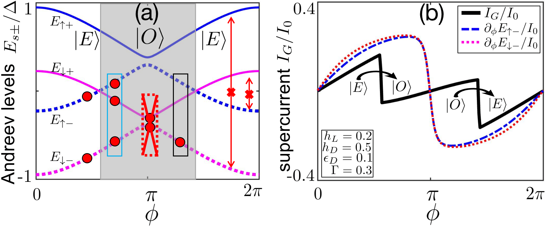
We study the singlet-doublet QPT resulting from the intricate competition between superconducting and spin-split proximity effects. The later promotes the doublet ground state akin to the quantum dot Coulomb repulsion. Note that an Andreev bound state of contributes to the supercurrent an amount , where is the charge of the electron and is the reduced Plank constant. Therefore, the underlying QPT manifests itself by a sudden change of the ground-state supercurrent [47, 48]. Figure 1(b) depicts the ground-state supercurrent as a function of . The sharp drop in the ground-state supercurrent occurs when a pair of Andreev levels cross zero [Fig. 1(a)]. The difference between solid and dashed curves of Fig. 1(b) unveils the unignorable contributions of continuous spectrum and hence it is necessary to include the continuous and subgap levels in the ground-state energy (9) to guarantee the uniqueness of the ground-state supercurrent. By following the logical framework based on an overcomplete basis set including both positive and negative orthonormal basis sets [47], we can either add the negative quasiparticle (cyan box) or remove the positive quasiparticle (black box) which switches fermionic parity [Eq. (8)] (see another explanation in Ref. [49]). However, we cannot do both (red box) because it violates the Pauli exclusion principle, i.e., . Quantitatively, the fermionic parity of the ground state changes in the presence of negative , as shown in Eq. (8). The first available negative , if present, is the Andreev level (10), whose iterative form simplifies the derivation of the critical conditions of the QPT, for example, critical dot energy
| (11) |
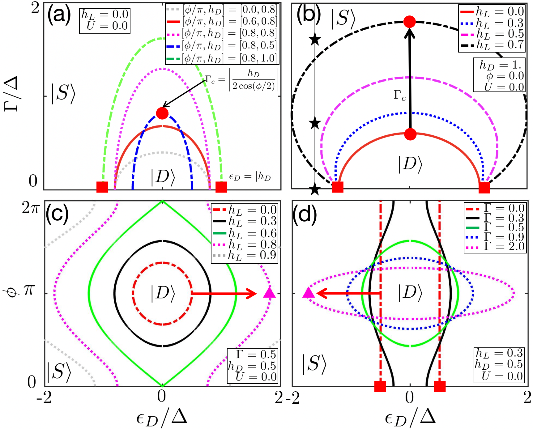
where . For , we obtain the critical magnetic field , whose renormalization effect distinguishes with the critical magnetic field of Ref. [9]. Figure 2 plots the phase diagram as a function of and (a,b) [(c,d) ]. The critical dot energy (11) reduces to at zero spin-split proximity effect (), where increasing always enhances the singlet phase and there is not doublet ground state anymore for larger than [circle in 2(a)]. Notably, we obtain the typical semicircle phase diagram [12, 13, 24], but in our case Coulomb interaction is not necessary. With increasing , we find larger [black arrow in 2(b)]. At , the superconducting proximity effects from two superconductors interfere destructively [Eq. (11)], while the spin-split proximity effect, surviving at , causes renormalization of the dot field. Then, Eq. (11) reduces to (triangles), which increases with and [red arrows in 2(c) and 2(d)]. The latter implies we can even enhance the doublet ground state by increasing for around [2(d)] which is opposite to the typical singlet-doublet QPT based on the quantum dot Coulomb interaction where strong tunnel coupling favors the singlet ground state. Moreover, this enhancement even happens at maximum superconducting proximity effect () owing to the strong spin-split proximity effect [black and magenta lines in 2(b)]. Our novel phase diagram, going beyond the typical phase diagram, allows a transition with increasing tunnel coupling [black stars in 2(b)]. Moreover, our iterative formalism allows for precise control of the ground-state phase. For example, we achieve pure doublet ground state for all [2(c) and 2(d)], which is crucial for the flux-tunable Andreev spin qubit.
III.3 QPT in the presence of Coulomb interaction
Though we obtain the semicircle phase diagram without Coulomb interaction [Fig. 2(a)], an unavoidable question is how to distinguish it with the typical semicircle phase diagram from Coulomb interaction in realistic experiments. Next, we include a quantum dot Coulomb interaction and study the Yu-Shiba-Rusinov case within the Hartree-Fock-Bogoliubov approximation [9, 18, 13]. The expressions of Andreev levels are given by the iterative form (see detailed derivations in Appendix B)
| (12) | ||||
The Coulomb interaction leads to the corrections in dot energy , dot field , and dot pair potential . Here, is the Fermi–Dirac distribution at temperature , where is the Boltzmann constant.
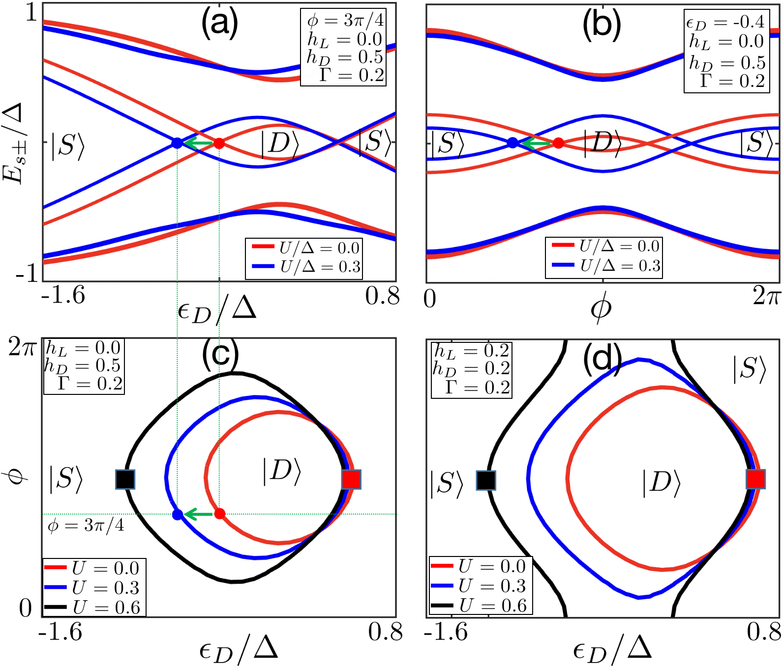
Figures 3 (a) and (b), respectively, plot the Andreev levels as a function of and . We see a clear zero-energy shift (green arrows) due to the Coulomb interaction preferring doublet ground state. This shift enhances the region of the doublet ground state as shown in Fig. 3 (c), which is further enhanced by the spin-split proximity effect () [Fig. 3 (d)]. Moreover, we find the Coulomb enhancement of the doublet ground state relies on the phase difference. Take as an example, where the superconducting proximity effects from two superconductors interfere destructively. We attain critical dot energy in small tunnel coupling, quantum dot energy, magnetic field, and Coulomb interaction limits (see detailed derivations in Appendix B)
| (13) |
Equation (13) at zero temperature reduces to , where the positive critical dot energy is almost independent of Coulomb interaction (red boxes), while the negative critical dot energy is shifted by Coulomb interaction (black boxes). Therefore, this QPT features with asymmetric behavior with dot energy , i.e., , enabling distinguish it from the symmetric QPT due to the interplay of superconducting and spin-split proximity effects (Fig. 2). Though this asymmetry can be artificially removed by redefining dot energy , i.e., , we can still use this effect in the experiments where the exact value of is known and controllable. For example, the asymmetry of the QPT with , in principle, offers an estimation of the quantum dot Coulomb interaction. The gate [50, 17, 11]-, field [18, 51]-, phase [35, 52]-tunable QPT has been observed in recent experiments. Though the experimental data are well explained by the Coulomb blockade, our theory might provide a more exhaustive illustration.
IV Conclusion
We highlight a renormalized and iterative expression of the Andreev level in a quantum-dot Josephson junction, which is bound to have significant implications due to several significant advantages as follows. Firstly, the iterative form of the Andreev level provides an intuitive understanding of the spin-split and superconducting proximity effects of the superconducting leads, while also effectively incorporating corrections for the effective quantum dot energy, magnetic field, and pair potential resulting from the quantum dot Coulomb interaction. Importantly, our iterative form of the Andreev level simplifies the analytical calculation of the critical conditions of the singlet-doublet QPT. Secondly, the renormalized form of the Andreev level not only allows us to extend beyond the limits of small tunnel coupling, quantum dot energy level, magnetic field, and Coulomb interaction but also enables the capture of subgap resonances that leak out of the superconducting gap into the continuous spectrum. These leaked subgap resonances are highly tunable by gate, phase, and field parameters and therefore play a significant role in the novel phenomena and remarkable properties of the superconductor. Last but not least, we derive the microscopic expressions for the transmission probability and the induced gap, which clearly shows the interaction between dot energy and superconducting proximity effect and works in the strong tunnel coupling, dot energy, and dot field limits.
V Acknowledgement
We sincerely thank Yugui Yao, Jose Carlos Egues, Junwei Liu, Gao Min Tang, Chuan Chang Zeng and Chun Yu Wan for helpful and sightful discussions. This work is supported by the National Natural Science Foundation of China (Grant Nos. 12234003, 12061131002), the National Key R&D Program of China (Grant No. 2020YFA0308800).
Appendix A Derivation of Andreev levels Eq. (5)
In this section, we diagonalize the hybrid quantum dot-superconducting lead system to obtain the compact expressions for the Andreev level energies given in Eq. (10) in the main text. Moreover, we show in detail the gate, phase, and field dependence of the Andreev levels.
We rewrite the total Hamiltonian (1) in overcomplete basis – the Nambu space of the hybrid quantum dot-superconductor system
| (14) |
where concatenates vertically. Thus, the total Hamiltonian (1) can be rewritten into the Bogoliubov–de Gennes (BdG) Hamiltonian in quadratic form
| (15) |
with
| (18) |
The prefactor and -independent constant energy arise from rewriting the total Hamiltonian (1) in overcomplete basis (14) [53]. is the corresponding Hamiltonian matrix in the Nambu space
| (21) |
Here, the dot energy and Zeeman energy correspond to the Pauli matrix and identity in the Nambu space, respectively. We consider only a single energy level on the dot, assuming that the level spacing to the next dot level is larger than all relevant energy scales. The superconducting lead Hamiltonian (3) in matrix form is given by
| (22) |
where concatenates diagonally. The quantum tunneling (4) reads
| (23) |
where concatenates vertically.
One can diagonalize the matrix of the BdG Hamiltonian (18)
| (24) |
where the transformation matrix is diagonal in spin space
| (27) |
is a unitary matrix, where is equal to half of the dimension of the Hamiltonian (21) and describes the size of the hybrid system. Hence, the BdG Hamiltonian (21) can be mathematically rewritten into
| (28) |
In the presence of superconductivity, we are required to work in the Nambu space doubling the Hilbert space, and hence an additional index labels the high/low energy levels of each spin species (), which satisfy . The larger corresponds to a higher energy level. Then, the terms with are Andreev levels – the subgap energy levels of the hybrid quantum dot and superconductor system and we here call all other energy levels () Bogoliubov levels – the out-of-gap energy levels of the hybrid system. The quasiparticle operator with energy is a unit vector in Nambu space of the hybrid system
| (29) |
Here, we define such that and for all . and , picked out from the unitary matrix , describe the electron and hole distributions of quasiparticles , respectively.
In general, it is hard to analytically calculate the energy levels of the hybrid system from the following determinant equation:
| (32) |
To find the Andreev (subgap) level, we can use the determinant identity for four matrices , and [54]:
| (33) |
where is assumed to be invertible. Thus, to use Eq. (33) to solve our determinant equation (32), is required to be invertible which is true for the Andreev levels (). Then, the determinant equation (32) reduces to
| (34) |
The self-energy in Eq. (34) is given by
| (35) |
The summation over momenta in Eq. (35) can be replaced by integration for the in-gap Andreev levels ,
| (36) |
where is the volume of the superconductor and is the density of states of superconductor per spin and energy band . There exist many bands with complex energy spectrum and we here assume energy-independent total density of state by setting for simplicity. Then, the self-energy (35) becomes
| (39) |
where and . We parameterize the tunnel coupling strength by . The in-gap requirement of the Andreev levels guarantees the invertible in determinat identity (33) and the integrable self-energy (39). Hence, one can derive the exact Andreev levels from Eq. (34) with the integrated self-energy (39). This procedure amounts to integrating out the superconducting degrees of freedom (which can be achieved in various ways).
Next, let us solve the reduced determinant equation (34). By substitution of Eq. (39), the reduced determinant equation (34) becomes
| (40) |
We can rewrite the above determinant equation into
| (41) | ||||
To better understand the superconducting proximity effect, we introduce the following dimensionless parameter
| (42) |
Thus, Eq. (41) reduces to
| (43) | ||||
with
| (44) |
The function renormalizes both Andreev levels and its spin splitting. Therefore, we have obtained a compact implicit equation from which we can easily obtain the Andreev levels explicitly by iterations
| (45) |
Considering the complexity of the expressions of Andreev levels (45), we first consider the case of . Then, Eq. (45) reduces to
| (46) | ||||
The interplay of the superconducting proximity effects from two superconducting leads is described by , which interferes destructively when and .
Hereafter, we set , , , and for simplicity. Thus, the Andreev levels (45) reduce to
| (47) |
with
| (48) |
For , we can obtain the spin-split Andreev levels from the spin-split superconductor, while the spin splitting of the quantum dot can be reduced by the superconducting proximity effect quantified by the renormalization factor [55]. At , the proximity effects from the two superconductors interfere destructively with each other. Thus, the Andreev levels (47) reduce to
| (49) |
While, in the absence of spin splitting (), the Andreev levels (47) become
| (50) |
with
| (51) |
We can find the exact expressions of transmission probability and induced gap (not pair potential), defined via ,
| (52) |
| (53) |
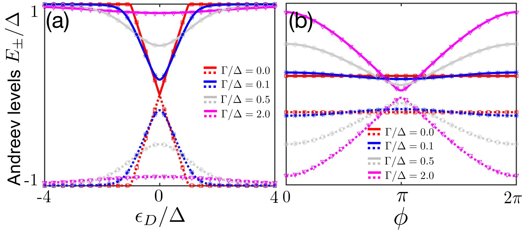
These expressions are useful for the quantification of microscopic parameters. Figure 4 (a) and (b) plot the zero-magnetic-field Andreev levels , numerically obtained from the diagonalization of Eq. (21), as a function of [] for different , respectively. The numerical Andreev energies agree well with the analytical Andreev energies (47) indicated by the star, square, circle, and triangle marks [Figs. 4 (a) and (b)].
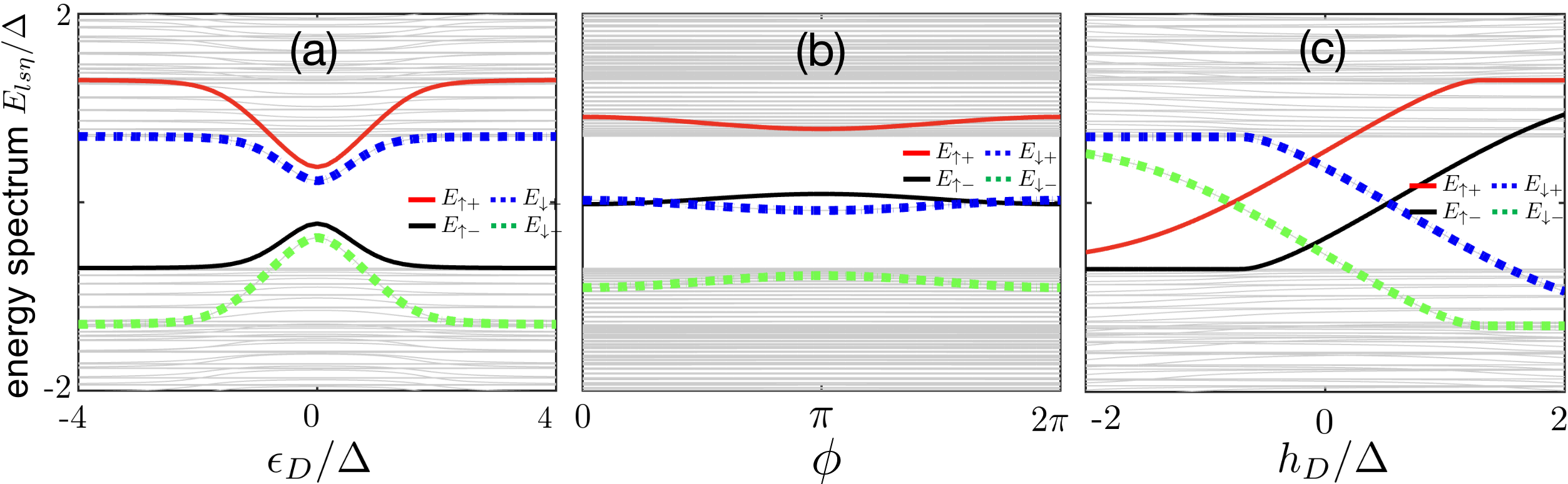
The Andreev levels (47) are renormalized by , making it possible to go beyond small tunnel coupling, dot energy, dot field, and Coulomb interaction limits. Figures 5 (a), (b), and (c) show plots of the energy levels as a function of (a) , (b) , and (c) , respectively. Qualitatively, the Andreev levels can be understood as coming form avoided crossing due to the tunneling between the quantum dot and superconducting leads. The avoided crossing of and bands results in a minigap of the Andreev levels at , while that of and bands repulse a bulk Bogoliubov level within the superconductor gap for . However, the avoided crossing of and bands results into a hysteresis-loop-like dependence [panel (c)]. Quantitatively, we try to attain some simplified expressions in several parameter regimes. In the limit of large gap, i.e., , we have and the Andreev levels (47) reduce to
| (54) |
The second term on the right-hand side of Eq. (54) describes the presence of the minigap of the Andreev levels at due to the avoided crossing of and bands [Fig. 5 (a)]. Next, we study the limit of large dot energy (), large dot field (), and large tunneling (), where the Andreev levels approach the gap edges when the phase difference is far away from . Thus, we have , and the Andreev levels (47), in second order of , take on the form
| (55) |
with . For , squaring Eq. (A) leads to
| (56) |
This describes the avoided crossing of and bands [Fig 5 (a)] and the avoided crossing of and bands [Fig 5 (c)]. Noting that becomes large when Andreev level approaches gap edges, the renormalization effect always forces the Andreev levels and inside even in large tunnel coupling, dot energy and dot field limits, as shown in Eq. (56). Moreover, the renormalization effect makes it works when two "subgap" levels, (red curve) and (green curve) in panels (a) and (b), leak out of the superconducting gap into the continuous part of the superconducting lead spectrum and , an effect that has no counterpart in the superconducting Anderson model [37]. These "subgap" levels are highly gate-, phase-, and field-tunable as plotted in Fig. 5, and hence play a significant role in superconducting properties, for example supercurrent noting that a quasiparticle state of contributes to the supercurrent an amount .
Appendix B Yu-Shiba-Rusinov case
In this section, we include Coulomb interaction and study the Yu-Shiba-Rusinov case using the Hartree-Fock-Bogoliubov approximation [9, 18, 13].
In the presence of Coulomb interaction, the dot Hamiltonian, reads
| (57) |
Here, is on-site Coulomb interaction and is number operator of the quantum dot with spin . Within the Hartree-Fock-Bogoliubov approximation, we reach
| (60) |
where means thermodynamic expectation. Thus, Coulomb interaction results in renormalization of dot energy, dot field, and dot pair potential
| (61) |
| (62) |
| (63) |
Following the same way of non-interacting case, we obtain Andreev Hamiltonian – the low-energy Hamiltonian of the hybrid quantum dot-nanowire-superconductor system
| (64) |
The expressions of Andreev levels are, again, given by iterative form
| (65) | ||||
To calculate the mean values in Eqs. (61-63), we derive the partition functions of the hybrid quantum dot and superconductor system [12]. The partition function of the hybrid system reads
| (66) |
The action, in partition function (66)
| (69) |
with
| (70) |
The Grassmann variables in Nambu space read
| (74) |
| (78) |
In principle, we are required to diagonalize Eq. (69) and attain partition function as follows
| (79) |
The mean values, in Eqs. (61-63), can be expressed by the Andreev partition function
| (80) |
| (81) |
| (82) |
Then, Coulomb interaction results in self-consistent equations
| (83) |
| (84) |
| (85) |
By substitution of Eq. (79), Eqs. (83-85) become
| (86) |
| (87) |
| (88) |
where we have used the relations
| (89) |
Here we can pick up anyone spin species.
Let us first switch off the quantum tunneling between quantum dot and superconductors. For , we have . Thus, Eq. (65) reduces to
| (90) |
and Eqs. (86) and (87) reduce to
| (91) |
| (92) |
We note that and hence we have
| (93) | ||||
| (94) | ||||
Therefore, both and are independent of . For . The QPT happens at . For positive , we have . By substitution of Eqs. (91) and (92), we find
| (95) |
which at zero temperature reduces to due to . For negative , we have . By substitution of Eqs. (91) and (92), we find
| (96) |
which at zero temperature reduces to due to .
Next, we switch on the quantum tunneling between the quantum dot and superconductors. Figs. 3 (a) and (b), respectively, plot the Andreev levels as a function of and in the presence of Coulomb interaction. We see a clear zero-energy shift (green arrows) due to the Coulomb interaction. This shift cause an enhancement of the region of the double ground state plotted in Figs. 3 (c) and (d), which plot the phase diagram as a function of and for and , respectively. The Coulomb interaction, preferring doublet, enhances the region of the doublet ground state [Fig. 3 (c)], which can be further enhanced by the spin-split proximity effect () [Fig. 3 (d)]. Moreover, we find the Coulomb enhancement of the doublet ground state depends on the phase difference, . Take as an example. The superconducting proximity effects from two superconductors interfere destructively. Thus, we have and the Andreev levels (65) reduces to
| (97) |
Read from Eq. (97), it is clear that we have
| (98) |
The QPT happens at zero Andreev levels. Without loss of generality, we set and we have at , where . Let us consider two cases. Let us begin with case. By substitution of Eqs. (86) and (87), we reach
| (99) |
Next, we study case. By substitution of Eqs. (86) and (87), we reach
| (100) | ||||
For simplicity, we consider weak tunnel coupling, small dot energy, and small Coulomb interaction limits, where the dot energy and field dependence of quasiparticle energy is dominated by Andreev levels, i.e.,
| (101) |
| (102) |
By substitution of Eq. (98), Eq. (99) becomes
| (103) |
which at zero temperature reduces to due to . Therefore, positive critical dot energy (103), at and K, is independent of but relies on , , and [red circles of Figs. 3 (c) and (d)]. Moreover, by substitution of Eq. (98), Eq. (100) becomes
| (104) |
which at zero temperature reduces to due to, again, . The negative critical dot energy (104) is shifted by Coulomb interaction [black circles of Figs. 3 (c) and (d)].
References
- Zazunov et al. [2003] A. Zazunov, V. Shumeiko, E. Bratus, J. Lantz, and G. Wendin, Andreev level qubit, Phys. Rev. Lett. 90, 087003 (2003).
- Janvier et al. [2015] C. Janvier, L. Tosi, L. Bretheau, Ç. Girit, M. Stern, P. Bertet, P. Joyez, D. Vion, D. Esteve, M. Goffman, et al., Coherent manipulation of andreev states in superconducting atomic contacts, Science 349, 1199 (2015).
- Bretheau et al. [2013a] L. Bretheau, Ç. Girit, C. Urbina, D. Esteve, and H. Pothier, Supercurrent spectroscopy of andreev states, Phys. Rev. X 3, 041034 (2013a).
- Bretheau et al. [2013b] L. Bretheau, Ç. Girit, H. Pothier, D. Esteve, and C. Urbina, Exciting andreev pairs in a superconducting atomic contact, Nature 499, 312 (2013b).
- Chtchelkatchev and Nazarov [2003] N. M. Chtchelkatchev and Y. V. Nazarov, Andreev quantum dots for spin manipulation, Phys. Rev. Lett. 90, 226806 (2003).
- Tosi et al. [2019] L. Tosi, C. Metzger, M. Goffman, C. Urbina, H. Pothier, S. Park, A. L. Yeyati, J. Nygård, and P. Krogstrup, Spin-orbit splitting of andreev states revealed by microwave spectroscopy, Phys. Rev. X 9, 011010 (2019).
- Hays et al. [2021] M. Hays, V. Fatemi, D. Bouman, J. Cerrillo, S. Diamond, K. Serniak, T. Connolly, P. Krogstrup, J. Nygård, A. L. Yeyati, A. Geresdi, and M. H. Devoret, Coherent manipulation of an andreev spin qubit, Science 373, 430 (2021).
- Wendin and Shumeiko [2021] G. Wendin and V. Shumeiko, Coherent manipulation of a spin qubit, Science 373, 390 (2021).
- Valentini et al. [2021] M. Valentini, F. Peñaranda, A. Hofmann, M. Brauns, R. Hauschild, P. Krogstrup, P. San-Jose, E. Prada, R. Aguado, and G. Katsaros, Nontopological zero-bias peaks in full-shell nanowires induced by flux-tunable andreev states, Science 373, 82 (2021).
- Franke et al. [2011] K. Franke, G. Schulze, and J. Pascual, Competition of superconducting phenomena and kondo screening at the nanoscale, Science 332, 940 (2011).
- Lee et al. [2017] E. J. Lee, X. Jiang, R. Aguado, C. M. Lieber, S. De Franceschi, et al., Scaling of subgap excitations in a superconductor-semiconductor nanowire quantum dot, Phys. Rev. B 95, 180502 (2017).
- Meng et al. [2009] T. Meng, S. Florens, and P. Simon, Self-consistent description of andreev bound states in josephson quantum dot devices, Phys. Rev. B 79, 224521 (2009).
- Vecino et al. [2003] E. Vecino, A. Martín-Rodero, and A. L. Yeyati, Josephson current through a correlated quantum level: Andreev states and junction behavior, Phys. Rev. B 68, 035105 (2003).
- Deacon et al. [2010] R. Deacon, Y. Tanaka, A. Oiwa, R. Sakano, K. Yoshida, K. Shibata, K. Hirakawa, and S. Tarucha, Tunneling spectroscopy of andreev energy levels in a quantum dot coupled to a superconductor, Phys. Rev. Lett. 104, 076805 (2010).
- Lim et al. [2015] J. S. Lim, R. López, R. Aguado, et al., Shiba states and zero-bias anomalies in the hybrid normal-superconductor anderson model, Phys. Rev. B 91, 045441 (2015).
- Higginbotham et al. [2015] A. P. Higginbotham, S. M. Albrecht, G. Kiršanskas, W. Chang, F. Kuemmeth, P. Krogstrup, T. S. Jespersen, J. Nygård, K. Flensberg, and C. M. Marcus, Parity lifetime of bound states in a proximitized semiconductor nanowire, Nat. Phys. 11, 1017 (2015).
- Jellinggaard et al. [2016] A. Jellinggaard, K. Grove-Rasmussen, M. H. Madsen, and J. Nygård, Tuning yu-shiba-rusinov states in a quantum dot, Phys. Rev. B 94, 064520 (2016).
- Lee et al. [2014] E. J. Lee, X. Jiang, M. Houzet, R. Aguado, C. M. Lieber, and S. De Franceschi, Spin-resolved andreev levels and parity crossings in hybrid superconductor–semiconductor nanostructures, Nat. Nanotechnol. 9, 79 (2014).
- Dvir et al. [2019] T. Dvir, M. Aprili, C. H. Quay, and H. Steinberg, Zeeman tunability of andreev bound states in van der waals tunnel barriers, Phys. Rev. Lett. 123, 217003 (2019).
- Lee et al. [2022] M. Lee, R. López, H. Q. Xu, and G. Platero, Proposal for detection of the and phases in quantum-dot josephson junctions, Phys. Rev. Lett. 129, 207701 (2022).
- Liu et al. [2019] Y. Liu, S. Vaitiekenas, S. Martí-Sánchez, C. Koch, S. Hart, Z. Cui, T. Kanne, S. A. Khan, R. Tanta, S. Upadhyay, et al., Semiconductor–ferromagnetic insulator–superconductor nanowires: Stray field and exchange field, Nano Lett. 20, 456 (2019).
- Vaitiekėnas et al. [2021] S. Vaitiekėnas, Y. Liu, P. Krogstrup, and C. Marcus, Zero-bias peaks at zero magnetic field in ferromagnetic hybrid nanowires, Nat. Phys. 17, 43 (2021).
- Kürtössy et al. [2021] O. Kürtössy, Z. Scherübl, G. Fülöp, I. E. Lukács, T. Kanne, J. Nygård, P. Makk, and S. Csonka, Andreev molecule in parallel InAs nanowires, Nano Lett. 21, 7929 (2021).
- Rozhkov and Arovas [1999] A. Rozhkov and D. P. Arovas, Josephson coupling through a magnetic impurity, Phys. Rev. Lett. 82, 2788 (1999).
- Bulla et al. [2008] R. Bulla, T. A. Costi, and T. Pruschke, Numerical renormalization group method for quantum impurity systems, Rev. Mod. Phys. 80, 395 (2008).
- Siano and Egger [2004] F. Siano and R. Egger, Josephson current through a nanoscale magnetic quantum dot, Phys. Rev. Lett. 93, 047002 (2004).
- Yeyati et al. [1997] A. L. Yeyati, J. Cuevas, A. López-Dávalos, and A. Martin-Rodero, Resonant tunneling through a small quantum dot coupled to superconducting leads, Phys. Rev. B 55, R6137 (1997).
- Martín-Rodero and Levy Yeyati [2011] A. Martín-Rodero and A. Levy Yeyati, Josephson and andreev transport through quantum dots, Adv. Phys. 60, 899 (2011).
- Yoshioka and Ohashi [2000] T. Yoshioka and Y. Ohashi, Numerical renormalization group studies on single impurity anderson model in superconductivity: A unified treatment of magnetic, nonmagnetic impurities, and resonance scattering, J. Phys. Soc. Jpn. 69, 1812 (2000).
- Karrasch et al. [2008] C. Karrasch, A. Oguri, and V. Meden, Josephson current through a single anderson impurity coupled to bcs leads, Phys. Rev. B 77, 024517 (2008).
- Wentzell et al. [2016] N. Wentzell, S. Florens, T. Meng, V. Meden, and S. Andergassen, Magnetoelectric spectroscopy of andreev bound states in josephson quantum dots, Phys. Rev. B 94, 085151 (2016).
- Kurilovich et al. [2021] P. D. Kurilovich, V. D. Kurilovich, V. Fatemi, M. H. Devoret, and L. I. Glazman, Microwave response of an andreev bound state, Phys. Rev. B 104, 174517 (2021).
- Bauer et al. [2007] J. Bauer, A. Oguri, and A. Hewson, Spectral properties of locally correlated electrons in a bardeen–cooper–schrieffer superconductor, J. Phys. Condens. Matter 19, 486211 (2007).
- Meden [2019] V. Meden, The anderson–josephson quantum dot—a theory perspective, J. Phys. Condens. Matter 31, 163001 (2019).
- Fatemi et al. [2021] V. Fatemi, P. Kurilovich, M. Hays, D. Bouman, T. Connolly, S. Diamond, N. Frattini, V. Kurilovich, P. Krogstrup, J. Nygard, et al., Microwave susceptibility observation of interacting many-body andreev states, arXiv:2112.05624 (2021).
- Zalom [2023] P. Zalom, Rigorous wilsonian renormalization group for impurity models with a spectral gap, Phys. Rev. B 108, 195123 (2023).
- Zalom and Žonda [2022] P. Zalom and M. Žonda, Subgap states spectroscopy in a quantum dot coupled to gapped hosts: Unified picture for superconductor and semiconductor bands, Phys. Rev.B 105, 205412 (2022).
- Pavešič et al. [2023] L. Pavešič, R. Aguado, and R. Žitko, Quantum dot josephson junctions in the strong-coupling limit, arXiv preprint arXiv:2304.12456 https://doi.org/10.48550/arXiv.2304.12456 (2023).
- van Gerven Oei et al. [2017] W.-V. van Gerven Oei, D. Tanasković, and R. Žitko, Magnetic impurities in spin-split superconductors, Phys. Rev.B 95, 085115 (2017).
- Kiršanskas et al. [2015] G. Kiršanskas, M. Goldstein, K. Flensberg, L. I. Glazman, and J. Paaske, Yu-shiba-rusinov states in phase-biased superconductor–quantum dot–superconductor junctions, Phys. Rev. B 92, 235422 (2015).
- Probst et al. [2016] B. Probst, F. Domínguez, A. Schroer, A. L. Yeyati, and P. Recher, Signatures of nonlocal cooper-pair transport and of a singlet-triplet transition in the critical current of a double-quantum-dot josephson junction, Phys. Rev. B 94, 155445 (2016).
- Larkin and Varlamov [2005] A. Larkin and A. Varlamov, Theory of fluctuations in superconductors (Clarendon Press, 2005).
- Fulde and Ferrell [1964] P. Fulde and R. A. Ferrell, Superconductivity in a strong spin-exchange field, Phys. Rev. 135, A550 (1964).
- Zhang et al. [2020] X. Zhang, V. Golovach, F. Giazotto, and F. Bergeret, Phase-controllable nonlocal spin polarization in proximitized nanowires, Phys. Rev. B 101, 180502 (2020).
- Bergeret et al. [2004] F. Bergeret, A. Volkov, and K. Efetov, Induced ferromagnetism due to superconductivity in superconductor-ferromagnet structures, Phys. Rev. B 69, 174504 (2004).
- De Gennes and Pincus [2018] P.-G. De Gennes and P. A. Pincus, Superconductivity of metals and alloys (CRC Press, 2018).
- Zhang and Yao [2024] X.-P. Zhang and Y. Yao, Fermi sea and sky in the bogoliubov-de gennes equation, arXiv preprint arXiv:2404.07423 https://doi.org/10.48550/arXiv.2404.07423 (2024).
- Zhang [2024] X.-P. Zhang, Fabry-perot superconducting diode, arXiv preprint arXiv:2404.08962 https://doi.org/10.48550/arXiv.2404.08962 (2024).
- Sakurai [1970] A. Sakurai, Comments on Superconductors with Magnetic Impurities, Prog. Theor. Phys. 44, 1472 (1970).
- Pillet et al. [2010] J. Pillet, C. Quay, P. Morfin, C. Bena, A. L. Yeyati, and P. Joyez, Andreev bound states in supercurrent-carrying carbon nanotubes revealed, Nat. Phys. 6, 965 (2010).
- Whiticar et al. [2021] A. Whiticar, A. Fornieri, A. Banerjee, A. Drachmann, S. Gronin, G. Gardner, T. Lindemann, M. Manfra, and C. Marcus, Zeeman-driven parity transitions in an andreev quantum dot, Phys. Rev. B 103, 245308 (2021).
- Chang et al. [2013] W. Chang, V. Manucharyan, T. Jespersen, J. Nygård, and C. Marcus, Tunneling spectroscopy of quasiparticle bound states in a spinful josephson junction, Phys. Rev. Lett. 110, 217005 (2013).
- Bernevig [2013] B. A. Bernevig, Topological insulators and topological superconductors, chapter 16, in Topological Insulators and Topological Superconductors (Princeton university press, 2013).
- Silvester [2000] J. R. Silvester, Determinants of block matrices, Math. Gaz. 84, 460 (2000).
- Futterer et al. [2013] D. Futterer, J. Swiebodzinski, M. Governale, and J. König, Renormalization effects in interacting quantum dots coupled to superconducting leads, Phys. Rev. B 87, 014509 (2013).