Mixture of partially linear experts
Abstract
In the mixture of experts model, a common assumption is the linearity between a response variable and covariates. While this assumption has theoretical and computational benefits, it may lead to suboptimal estimates by overlooking potential nonlinear relationships among the variables. To address this limitation, we propose a partially linear structure that incorporates unspecified functions to capture nonlinear relationships. We establish the identifiability of the proposed model under mild conditions and introduce a practical estimation algorithm. We present the performance of our approach through numerical studies, including simulations and real data analysis.
Keywords: Machine learning, Mixture of experts, Model-based clustering, Partially linear models
1 Introduction
Quandt (1972) introduced a finite mixture of regressions (FMR) for uncovering hidden latent structures in data. It assumes the existence of unobserved subgroups, each characterized by distinct regression coefficients. Since the introduction of FMR, extensive research has been conducted to enhance its performance, with contributions from Neykov et al. (2007), Bai et al. (2012), Bashir and Carter (2012), Hunter and Young (2012), Yao et al. (2014), Song et al. (2014), Zeller et al. (2016), Zeller et al. (2019), Ma et al. (2021), Zarei et al. (2023), and Oh and Seo (2024).
However, because FMRs assume that the assignment of each data point to clusters is independent of the covariates (Hennig, 2000), FMR can be undermined with regard to the performance of regression clustering when the assumption of assignment independence is violated. Alternatively, Jacobs et al. (1991) introduced the mixture of linear experts (MoE), allowing for the assignment of each data point to depend on the covariates. Nguyen and McLachlan (2016) suggested the Laplace distribution for the error distributions, while Chamroukhi (2016) and Chamroukhi (2017) used distributions and skew- distributions for errors, respectively. Murphy and Murphy (2020) further extended MoE with a parsimonious structure to improve estimation efficiency. Mirfarah et al. (2021) introduced the use of scale mixture of normal distributions for errors within MoE. Recently, Oh and Seo (2023) proposed a specific MoE variant, assuming that covariates follow finite Gaussian location-scale mixture distributions and that the response follows finite Gaussian scale mixture distributions.
In spite of extra flexibility for errors in these models, they assumed linear structures in each mixture component, which makes too simple to capture the hidden latent structures. In homogeneous population, Engle et al. (1986) introduced a partial linear model, comprising a response variable is represented as a linear combination of specific -dimensional covariates and an unspecified non-parametric function that includes an additional covariate , as follows.
| (1) |
where , is an error term with a mean zero and finite variance, and the function is an unknown non-parametric function. This model has the advantages of interpretability, stemming from its linearity, with the flexibility to capture diverse functional relationships through an unspecified function . The differentiation between and U is determined either theoretically based on established knowledge in the application field or through methods like scatter plots or statistical hypothesis testing. Wu and Liu (2017) and Skhosana et al. (2023) suggested the FMR to accommodate a partially linear structure within a heterogeneous population.
In this paper, we consider a novel approach that incorporates partially linear structures into MoE, utilizing unspecified functions based on kernel methods. This allows proposed model to effectively capture various relationships between the response and covariates, while latent variable is dependent on some covariates. This flexibility can significantly impact the estimation of regression coefficients and enhance clustering performance by mitigating misspecification problems arising from assumptions about the relationships between variables. In addition, we address the issue of identifiability in the proposed model to ensure the reliability of the outcomes derived from proposed approach.
The remainder of this paper is organized as follows. Section 2 reviews MoE and introduces the proposed models, addressing the identifiability. Section 3 outlines the estimation procedure, while Section 4 deals with practical issues related to the proposed models. We present the results of simulation studies in Section 5 and apply the models to real datasets in Section 6. Finally, we provide a discussion in Section 7.
2 Semiparametric mixture of partially linear experts
2.1 Mixture of linear experts
Let be a latent variable indicating the membership of the observations. MoE is a useful tool when exploring the relationship between the response variable and covariates in the presence of unobserved information about heterogeneous subpopulations by latent variable . Jacobs et al. (1991) presented the conditional probability distribution of the response variable given the covariates as
| (2) |
where , , represents a mixing probability that depends on the given covariates, with and . Additionally, represents a -dimensional vector for , and denotes the probability density function of the normal distribution with mean and variance .
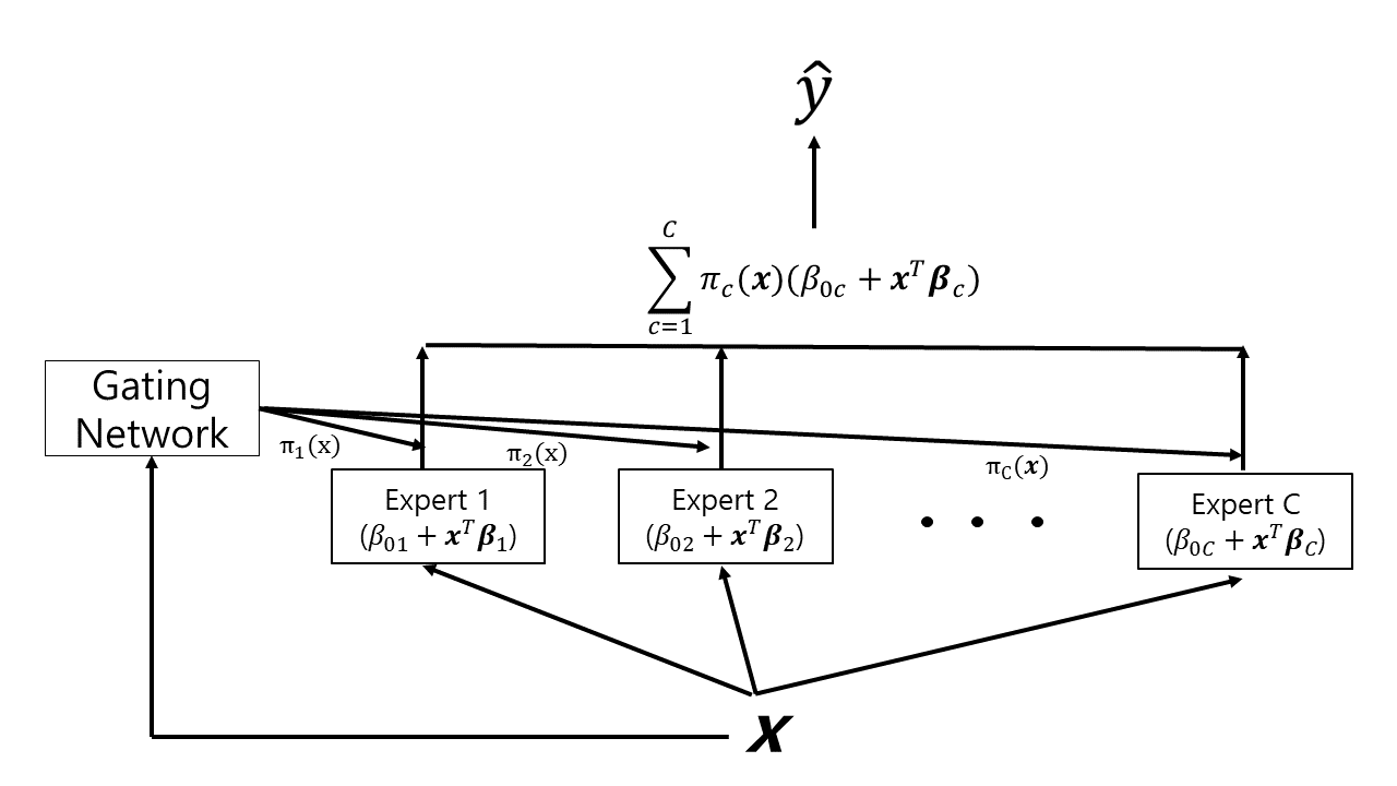
Regression clustering, the process of identifying the latent variable , holds significant importance in understanding the prediction mechanism employed by MoE. The predicted value of the response variable for new covariate is determined as
where is often called as the gating network, while is referred to as the expert network. That is, the prediction structure can be understood as an ensemble model as shown in Figure 1 because the predicted values are obtained by combining the outcomes of the expert networks using the gating network. Consequently, selecting an appropriate latent variable is a crucial aspect of the MoE model.
MoE is applied in various fields as a machine learning model. For example, Li et al. (2019) used MoE to explain differences in lane-changing behavior based on driver characteristics. Shen et al. (2019) extended MoE to adapt to the characteristics of data for creating a translation model capable of various translation styles. Additionally, Riquelme et al. (2021) proposed Vision MoE, which maintains superior performance compared to existing models in image classification while significantly reducing estimation time.
2.2 Proposed model
In this section, we introduce a semiparametric mixture of partially linear experts (MoPLE) model. The MoPLE is constructed by considering each expert network of the MoE model as a partial linear model (1), which can be defined as
| (3) |
Here, is defined as , where represents a -dimensional vector (), especially with being a zero vector. When , since is equal to , (3) simply represents a partial linear model (1). If and , (3) is equivalent to the MoE (2).
Identifiability is a fundamental concern when dealing with finite mixture models. Hennig (2000) established that finite mixture of regressions is identifiable when the domain of includes an open set in .
Additionally, Huang and Yao (2012) demonstrated that (2), with unspecified for , is identifiable up to a permutation of relabeling.
Furthermore, Wu and Liu (2017) extended these findings by establishing the identifiability of the mixture of partially linear regressions, assuming that is a zero vector in (3).
Building upon these results, the following theorem establishes the identifiability of model (3).
Theorem 1.
Suppose that the functions , , are continuous, and the parameter vectors are distinct in for . Additionally, assume that the covariate does not contain a constant, and none of its components can be a deterministic function of . If the support of contains an open set in , then (3) is identifiable up to a permutation of its components for almost all .
Proof.
In (3), suppose that there exist , , and , , satisfying
| (4) |
where (), , are distinct. Consider the set for any and (, ), where and , for a given . This set represents a -dimensional hyperplane in . For any pair of and with and , the union of a finite number of such hyperplanes, where , has a zero Lebesgue measure in . This fact remains true for the finite number of sets for any and (, ), where and for given .
From Lemma 1 of Huang and Yao (2012), it can be established that (4) is identifiable when conditioned on , under the condition that both sets of for and for are distinct. That is, if is given, we obtain , and there exists a permutation among the finite number of possible permutations of such that
where .
Now, let us consider any permutation that satisfies
| (5) |
for some , and verify that has to be unique . Suppose that and . This contradicts to the assumption that cannot be a deterministic function of . When and , the set has zero Lebesgue measure since it is a dimensional hyperplane in . Because indicates , we obtain that
for . Since the parameter sets and for are distinct, the permutation , satisfying (5) on a subset of the support of with nonzero Lebesgue measure, is unique.
Because and are continuous and one to one function, it follows that for . Moreover, as cannot be a constant, must be hold. Consequently, this indicates , except for the set , which has a zero Lebesgue measure in , for . Therefore, we can conclude that (3) is identifiable up to a permutation of its components. ∎
3 Estimation
When considering the observed data , the log-likelihood function is defined as
| (6) |
where is the set of all parameters and . To find and that maximize equation (6), we propose the Expectation Conditional Maximization (ECM) algorithm (Meng and Rubin, 1993) using the profile likelihood method. The latent indicator variable (), which indicates to which latent cluster the observed values belong, and the complete log-likelihood function are respectively defined as
and
In the E-step for the th iteration of the ECM algorithm, , we obtain using the posterior probability given and , which is represented as
While keeping fixed, CM-step 1 involves updating to that maximizes the following local likelihood:
where , and represents the kernel weighting function with bandwidth . Consequently, can be calculated as
In CM-step 2, after fixing , we can determine as follows.
Here, , , is a diagonal matrix with diagonal elements , is a identity matrix, and is a matrix with elements defined as
4 Practical issues
In practice, it is recommend to explore multiple initial values when employing the ECM algorithm, as the mixture likelihood inherently exhibits multimodality. To acquire appropriate initial values, we utilize the mixture of linear experts approach as proposed by Jacobs et al. (1991) for parameters such as , , , , and , where . Specifically, we set as in (2) when employing the mixture of linear experts, where . Multiple initial values are then selected by repeating the process of generating initial values and choosing the ones with the highest likelihood. In this study, we repeat this process 10 times to ensure the acquisition of suitable initial values.
Furthermore, it is crucial to employ suitable methods for determining the optimal number of mixture components. In this paper, we utilized the Bayesian information criterion (BIC; Schwarz 1978) obtained as , where is the log-likelihood function and is degree of freedoms, to select the number of components. However, directly applying the BIC to the proposed model is challenging due to the complexity of calculating degrees of freedom, particularly in the presence of non-parametric functions. Therefore, we adopt a modified approach for determining degrees of freedom, inspired by Wu and Liu (2017), as follows.
where represents the support of the non-parametric component covariates and
Given that the degrees of freedom depends on the bandwidth, we chose the bandwidth associated with the lowest BIC among the candidates.
5 Simulaton studies
In this section, we present simulation results demonstrating the performance of the proposed method compared to other estimation methods under various cases. Specifically, we consider the following methods for each simulated sample:
-
1.
MoE: Mixture of linear experts
-
2.
FMPLR: Finite mixture of partially linear regressions.
-
3.
MoPLE: Mixture of partially linear experts.
FMPLR was introduced by Wu and Liu (2017), where it is assumed that all to be zero vectors. We utilize the MoEClust in R package (Murphy and Murphy, 2022) for MoE, while we implement our R program for FMPLR and MoPLE.
We conduct three simulation scenarios, each comprising two mixture components as detailed in Table 1. In each of these experiments, we assume that the covariates and are independent random variables following a standard uniform distribution. In the first experiment, we assume a linear relationship between and within each mixture component, with the probability of observations belonging to latent clusters dependent on . In the second experiment, we introduce partially linear relationships between and while keeping the probability of observations belonging to latent clusters independent of . In the third experiment, we also consider partially linear relationships, but it features the probability of observations belonging to latent clusters as dependent on . Hence, we can expect that MoE, FMPLR and MoPLE represent efficient methods for Case , Case , and Case , respectively.
| Scenarios | Gating Network | Component | Component | |||||
|---|---|---|---|---|---|---|---|---|
| Case | -0.5 | 2 | -3 | -3u | 0.5 | 3 | 3u | 0.25 |
| Case | 0 | 0 | -3 | 0.5 | 3 | 0.25 | ||
| Case | -0.5 | 2 | -3 | 0.5 | 3 | 0.25 | ||
| Method | ARI | AMI | |||||
|---|---|---|---|---|---|---|---|
| MSE (bias) | MSE (bias) | MAE | MAE | ||||
| MoE | (0.016) | (0.005) | |||||
| (0.010) | (-0.005) | ||||||
| (-0.003) | (-0.005) | ||||||
| FMPLR | 0.049 (-0.033) | 0.040 (-0.023) | 0.159 | 0.130 | 0.952 | 0.908 | |
| 0.026 (-0.004) | 0.019 (-0.034) | 0.113 | 0.093 | 0.954 | 0.908 | ||
| 0.014 (-0.051) | 0.010 (-0.032) | 0.084 | 0.070 | 0.955 | 0.910 | ||
| MoPLE | 0.047 (0.014) | 0.040 (0.006) | 0.154 | 0.127 | 0.960 | 0.920 | |
| 0.024 (0.011) | 0.018 (-0.006) | 0.110 | 0.089 | 0.961 | 0.921 | ||
| 0.011 (-0.001) | 0.051 (-0.016) | 0.082 | 0.081 | 0.961 | 0.920 |
| Method | ARI | AMI | |||||
|---|---|---|---|---|---|---|---|
| MSE (bias) | MSE (bias) | MAE | MAE | ||||
| MoE | 0.077 (-0.062) | 0.120 (-0.036) | 0.362 | 1.056 | 0.652 | 0.562 | |
| 0.041 (-0.079) | 0.056 (-0.033) | 0.361 | 1.063 | 0.657 | 0.562 | ||
| 0.019 (-0.053) | 0.030 (-0.033) | 0.356 | 1.063 | 0.664 | 0.565 | ||
| FMPLR | (0.014) | (0.015) | 0.231 | 0.639 | |||
| 0.079 (0.026) | 0.043 (0.005) | 0.126 | 0.204 | 0.741 | 0.643 | ||
| 0.033 (0.040) | (0.001) | 0.160 | 0.748 | 0.649 | |||
| MoPLE | (0.014) | (0.012) | 0.734 | ||||
| (0.006) | (0.010) | ||||||
| (0.029) | (-0.013) |
| Method | ARI | AMI | |||||
|---|---|---|---|---|---|---|---|
| MSE (bias) | MSE (bias) | MAE | MAE | ||||
| MoE | (-0.074) | 0.230 (-0.169) | 0.361 | 1.100 | 0.641 | 0.529 | |
| (-0.079) | 0.127 (-0.175) | 0.357 | 1.074 | 0.645 | 0.529 | ||
| 0.020 (-0.076) | 0.087 (-0.207) | 0.348 | 1.0578 | 0.652 | 0.533 | ||
| FMPLR | 0.078 (-0.118) | 0.215 (-0.170) | 0.182 | 0.270 | 0.661 | 0.556 | |
| 0.044 (-0.132) | 0.075 (-0.130) | 0.146 | 0.203 | 0.671 | 0.562 | ||
| 0.036 (-0.123) | 0.075 (-0.145) | 0.125 | 0.193 | 0.675 | 0.566 | ||
| MoPLE | (0.038) | (-0.020) | |||||
| (0.038) | (-0.039) | ||||||
| (0.038) | (-0.045) |
The performance of each method is evaluated by calculating the bias as and mean square error (MSE) as , where and are the true regression coefficient in th expert network and the estimate of the from the th sample for and , respectively, for every regression parameter across a total of replicated samples, with sample sizes of 250, 500 and 1000. To assess the quality of the estimated nonparametric function for , we utilize the mean absolute error (MAE) defined as
where . We chose as grid points evenly distributed within the range of the covariate , with set to 100. We employ the Epanechnikov kernel function and determine regression clusters for observations using the maximum a posteriori. To assess the clustering performance, the Adjusted Rand Index (ARI, Hubert and Arabie, 1985) and Adjusted Mutual Information (AMI, Vinh et al., 2009) are computed. Note that smaller values of bias, MSE and MAE indicate better performance, while larger values of ARI and AMI signify better performance.
In Case , MoE exhibits the best performance across all criteria, while MoPLE ranks second in terms of clustering performance. In Case , MoPLE performs the best in terms of ARI and AMI, while FMPLR and MoPLE are competitive with regard to the estimating parameters. In Case , MoPLE demonstrates the best with regard to almost all criteria compared to the other methods. Overall, MoPLE demonstrates competitive performance, ranking either as the best or the second best method across all cases.
6 Real data analysis
6.1 Prestige dataset
For the first real data analysis, we consider the Prestige dataset, which is available in the car package in R. It comprises 102 observations with the variable such as Prestige, indicating occupational prestige from a mid-1960s social survey, Education, representing the average years of education for workers in 1971, Income, denoting the standardized average income of workers in 1971, and Occupational types, specifying occupational categories like professional, white-collar, and blue-collar occupations. In this study, we model the response variable as Prestige, where represents Education, and represents Income. Additionally, we assume that the latent variable is associated with Occupational types.
Table 5 displays the BIC values obtained by each method for the Prestige dataset. MoPLE correctly selects the expected number of components, while MoE and FMPLR yield fewer clusters than expected. The clustering performance of each method is summarized in Table 6. MoE performs the best in terms of ARI, whereas MoPLE excels in terms of AMI. As a result, MoPLE is considered the best method since it not only produces the expected number of clusters but also delivers competitive clustering performance. MoE is the second-best method, despite not selecting the expected number of clusters. This suggests that occupational types are dependent on education, and there are nonlinear relationships between prestige and income, at least within one component.
| Number of clusters | MoE | FMPLR | MoPLE |
|---|---|---|---|
| 1 | 724.22 | 947.23 | 947.23 |
| 2 | 852.19 | ||
| 3 | 735.49 | 951.21 | |
| 4 | 736.40 | 1042.96 | 1126.14 |
| 5 | 763.94 | 1633.26 | 1186.94 |
| Index | MoE | FMPLR | MoPLE |
|---|---|---|---|
| ARI | 0.0597 | 0.4779 | |
| AMI | 0.4012 | 0.0725 |
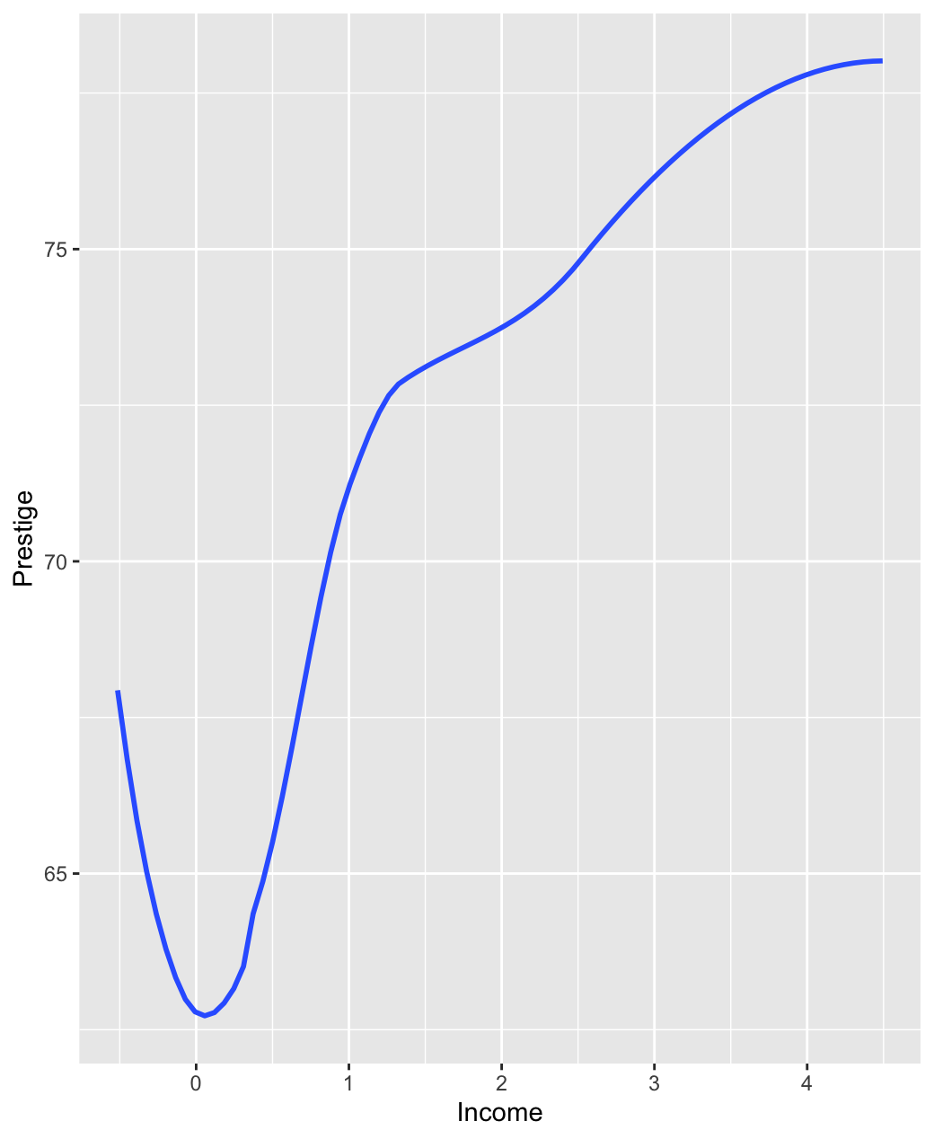
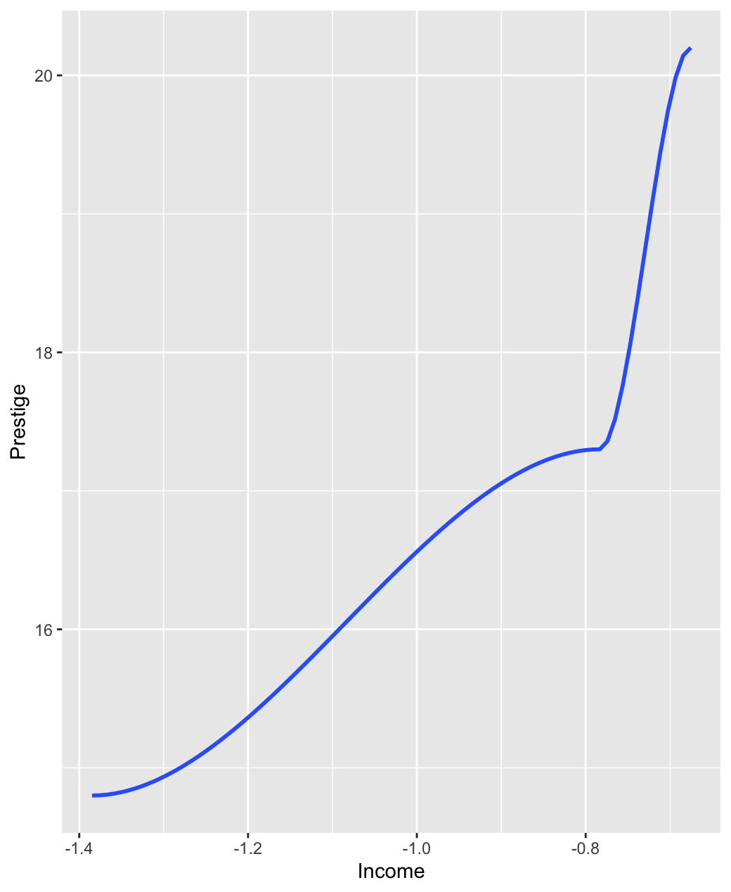
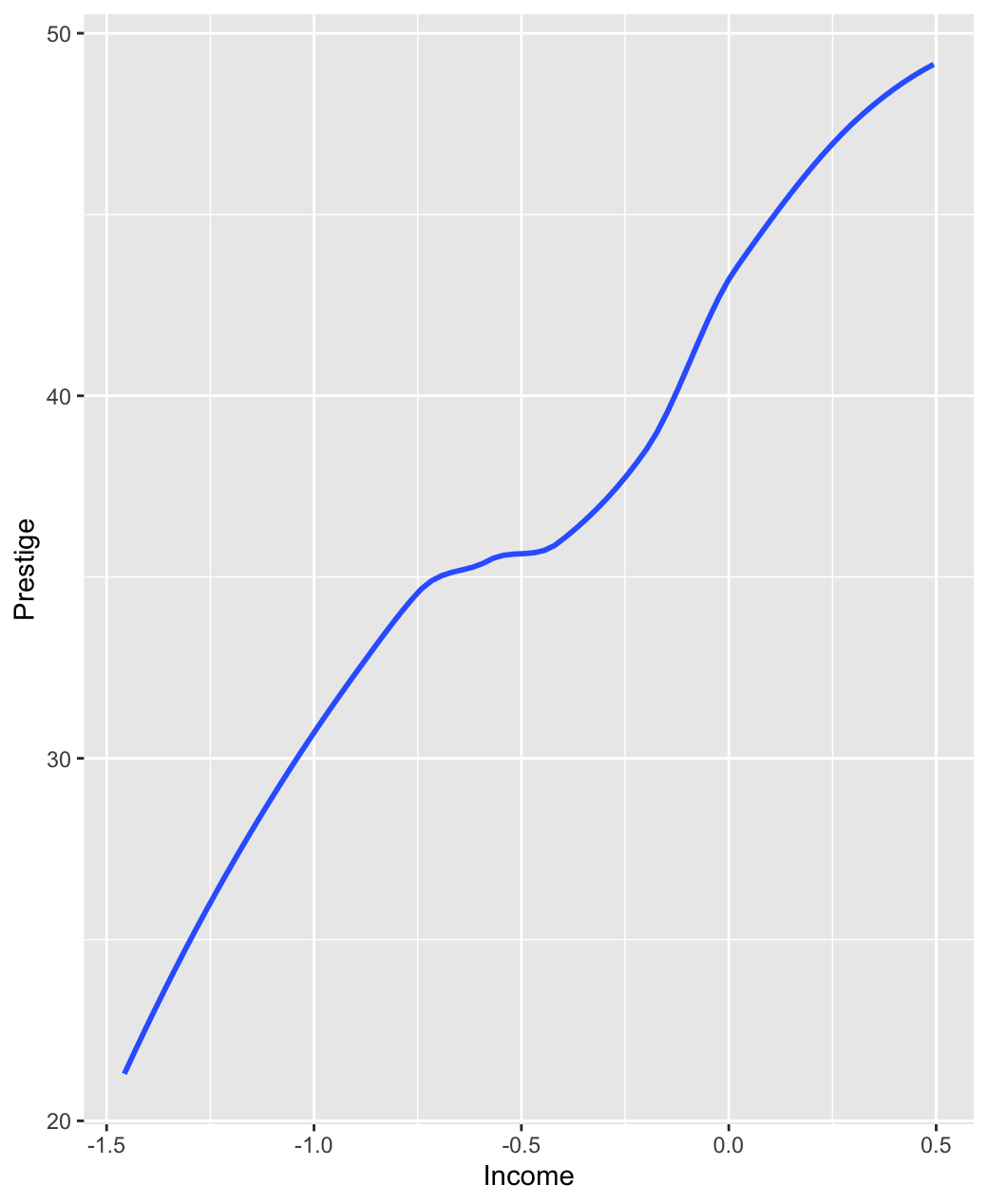
Based on the findings from MoPLE, the clusters denoted as , , and correspond to professional, white-collar, and blue-collar occupations, respectively. The estimated coefficients for the Education in Class 1, 2, and 3 are 2.331, 5.446, and 2.547, respectively. This suggests that the impact of the education on the prestige is most pronounced in white-collar. Figure 2 illustrates the estimated for each cluster, where . We note a nonlinear association between prestige and income within cluster , whereas clusters and exhibit a positive relationship between prestige and income, indicating an increasing trend.
6.2 Gross domestic product dataset
In the second real data analysis, we examine gross domestic product (GDP) dataset sourced from the STARS database of World Bank. This dataset comprises information from 82 countries over the period 1960 to 1987 and includes some variables such as (GDP), indicating logarithm of real gross domestic product in million dollars, (Labor), representing logarithm of the economically active population aged 15 to 65, (Capital), implying logarithm of the estimated initial capital stock in each country, and (Education), denoting logarithm of the average years of education.
Previously, researchers such as Duffy and Papageorgiou (2000) utilized this dataset to investigate the Cobb-Douglas specification, while Wu and Liu (2017) examined how education and two other variables influence GDP using FMPLR with a fixed two-component mixture. In this paper, we investigate countries in 1975 with , and , comparing clustering performance. To evaluate the clustering performance, we introduce a latent variable that indicates whether the country was classified as advanced or developing in 1975 based on International Monetary Fund (IMF).
| Number of clusters | MoE | FMPLR | MoPLE |
|---|---|---|---|
| 1 | 74.46 | 337.10 | 337.10 |
| 2 | 88.05 | 176.92 | |
| 3 | 178.15 | ||
| 4 | 114.48 | 265.12 | 232.49 |
| 5 | 110.04 | 419.94 | 405.89 |
| Index | MoE | FMPLR | MoPLE |
|---|---|---|---|
| ARI | 0.3449 | -0.1238 | |
| AMI | 0.3280 | 0.1042 |
Table 7 and Table 8 present the BIC values and clustering performance, respectively. In Table 7, MoPLE yield the expected number of clusters, while MoE and FMPLR selects more clusters than expected. In Table 8, MoPLE achieves the best results in terms of both ARI and AMI, followed by MoE. These findings suggest that MoPLE is the most suitable method when attempting to identify clusters among countries based on their classification as advanced or developing.
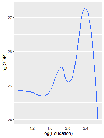
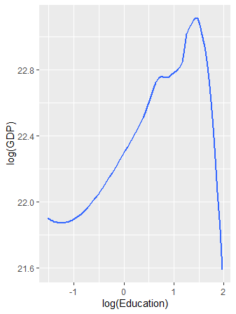
According to the results derived from MoPLE, the clusters labeled as and represent advanced and developing countries, respectively. In addition, cluster reveals estimated coefficients for and as , while cluster displays coefficients as . These results suggest that the impact of labor and capital on GDP does not significantly differ between advanced and developing countries. Figure 3 depicts the estimated for each cluster, with . Specifically, in cluster , the values of (GDP) appear to be higher compared to those in cluster , while their shapes look similar.
7 Discussion
In this paper, we propose MoPLE, which applies a partial linear structrure to the expert network of MoE, replacing the linear structure. In numerical studies, MoPLE demonstrates the ability to estimate both parametric and non-parametric components effectively, not only under linear relationships between the response variable and covariates but also under non-linear relationships. Furthermore, it gives comparative performance in terms of the regression clustering. These results imply that MoPLE is a valuable model regardless of whether the data exhibits linear or non-linear relationships, excelling not only in parameter estimation but also in clustering.
While this study assumed univariate covariates for the non-parametric component, it is possible to extend this approach to higher dimensions. Nevertheless, we must acknowledge the curse of dimensionality as a limitation of non-parametric methods. One potential alternative approach is to structure each expert as a partially linear additive model. Furthermore, although we postulate a specified variable following nonlinear relationships based on the previous work, it is still necessary to construct statistical hypothesis tests for nonlinear relationships, even though it may be challenging due to the presence of a hidden latent structure.
References
- Bai et al. (2012) Bai, X., Yao, W., and Boyer, J. E. (2012). Robust fitting of mixture regression models. Computational Statistics & Data Analysis, 56(7):2347–2359.
- Bashir and Carter (2012) Bashir, S. and Carter, E. (2012). Robust mixture of linear regression models. Communications in Statistics-Theory and Methods, 41(18):3371–3388.
- Chamroukhi (2016) Chamroukhi, F. (2016). Robust mixture of experts modeling using the t distribution. Neural Networks, 79:20–36.
- Chamroukhi (2017) Chamroukhi, F. (2017). Skew t mixture of experts. Neurocomputing, 266:390–408.
- Duffy and Papageorgiou (2000) Duffy, J. and Papageorgiou, C. (2000). A cross-country empirical investigation of the aggregate production function specification. Journal of Economic Growth, 5(1):87–120.
- Engle et al. (1986) Engle, R. F., Granger, C. W., Rice, J., and Weiss, A. (1986). Semiparametric estimates of the relation between weather and electricity sales. Journal of the American statistical Association, 81(394):310–320.
- Hennig (2000) Hennig, C. (2000). Identifiablity of models for clusterwise linear regression. Journal of Classification, 17(2):273–296.
- Huang and Yao (2012) Huang, M. and Yao, W. (2012). Mixture of regression models with varying mixing proportions: a semiparametric approach. Journal of the American Statistical Association, 107(498):711–724.
- Hunter and Young (2012) Hunter, D. R. and Young, D. S. (2012). Semiparametric mixtures of regressions. Journal of Nonparametric Statistics, 24(1):19–38.
- Jacobs et al. (1991) Jacobs, R. A., Jordan, M. I., Nowlan, S. J., and Hinton, G. E. (1991). Adaptive mixtures of local experts. Neural computation, 3(1):79–87.
- Li et al. (2019) Li, G., Pan, Y., Yang, Z., and Ma, J. (2019). Modeling vehicle merging position selection behaviors based on a finite mixture of linear regression models. IEEE Access, 7:158445–158458.
- Ma et al. (2021) Ma, Y., Wang, S., Xu, L., and Yao, W. (2021). Semiparametric mixture regression with unspecified error distributions. Test, 30(2):429–444.
- Meng and Rubin (1993) Meng, X.-L. and Rubin, D. B. (1993). Maximum likelihood estimation via the ecm algorithm: A general framework. Biometrika, 80(2):267–278.
- Mirfarah et al. (2021) Mirfarah, E., Naderi, M., and Chen, D.-G. (2021). Mixture of linear experts model for censored data: A novel approach with scale-mixture of normal distributions. Computational Statistics & Data Analysis, 158:107182.
- Murphy and Murphy (2020) Murphy, K. and Murphy, T. B. (2020). Gaussian parsimonious clustering models with covariates and a noise component. Advances in Data Analysis and Classification, 14(2):293–325.
- Murphy and Murphy (2022) Murphy, K. and Murphy, T. B. (2022). Package ‘MoEClust’. CRAN.
- Neykov et al. (2007) Neykov, N., Filzmoser, P., Dimova, R., and Neytchev, P. (2007). Robust fitting of mixtures using the trimmed likelihood estimator. Computational Statistics & Data Analysis, 52(1):299–308.
- Nguyen and McLachlan (2016) Nguyen, H. D. and McLachlan, G. J. (2016). Laplace mixture of linear experts. Computational Statistics & Data Analysis, 93:177–191.
- Oh and Seo (2023) Oh, S. and Seo, B. (2023). Merging components in linear gaussian cluster-weighted models. Journal of Classification, 40:25–51.
- Oh and Seo (2024) Oh, S. and Seo, B. (2024). Semiparametric mixture of linear regressions with nonparametric gaussian scale mixture errors. Advances in Data Analysis and Classification, 18:5–31.
- Quandt (1972) Quandt, R. E. (1972). A new approach to estimating switching regressions. Journal of the American statistical association, 67(338):306–310.
- Riquelme et al. (2021) Riquelme, C., Puigcerver, J., Mustafa, B., Neumann, M., Jenatton, R., Susano Pinto, A., Keysers, D., and Houlsby, N. (2021). Scaling vision with sparse mixture of experts. Advances in Neural Information Processing Systems, 34:8583–8595.
- Schwarz (1978) Schwarz, G. (1978). Estimating the dimension of a model. Annals of statistics, 6(2):461–464.
- Shen et al. (2019) Shen, T., Ott, M., Auli, M., and Ranzato, M. (2019). Mixture models for diverse machine translation: Tricks of the trade. Proceedings of the 36th International Conference on Machine Learning, 97:5719–5728.
- Skhosana et al. (2023) Skhosana, S. B., Millard, S. M., and Kanfer, F. H. (2023). A novel em-type algorithm to estimate semi-parametric mixtures of partially linear models. Mathematics, 11(5):1087.
- Song et al. (2014) Song, W., Yao, W., and Xing, Y. (2014). Robust mixture regression model fitting by laplace distribution. Computational Statistics & Data Analysis, 71:128–137.
- Wu and Liu (2017) Wu, X. and Liu, T. (2017). Estimation and testing for semiparametric mixtures of partially linear models. Communications in Statistics-Theory and Methods, 46(17):8690–8705.
- Yao et al. (2014) Yao, W., Wei, Y., and Yu, C. (2014). Robust mixture regression using the t-distribution. Computational Statistics & Data Analysis, 71:116–127.
- Zarei et al. (2023) Zarei, A., Khodadadi, Z., Maleki, M., and Zare, K. (2023). Robust mixture regression modeling based on two-piece scale mixtures of normal distributions. Advances in Data Analysis and Classification, 17:181–210.
- Zeller et al. (2016) Zeller, C. B., Cabral, C. R. B., and Lachos, V. H. (2016). Robust mixture regression modeling based on scale mixtures of skew-normal distributions. TEST, 25(2):375–396.
- Zeller et al. (2019) Zeller, C. B., Cabral, C. R. B., Lachos, V. H., and Benites, L. (2019). Finite mixture of regression models for censored data based on scale mixtures of normal distributions. Advances in Data Analysis and Classification, 13:89–116.