Distributed Structured Matrix Multiplication
Abstract
We devise achievable encoding schemes for distributed source compression for computing inner products, symmetric matrix products, and more generally, square matrix products, which are a class of nonlinear transformations. To that end, our approach relies on devising nonlinear mappings of distributed sources, which are then followed by the structured linear encoding scheme, introduced by Körner and Marton. For different computation scenarios, we contrast our findings on the achievable sum rate with the state of the art to demonstrate the possible savings in compression rate. When the sources have special correlation structures, it is possible to achieve unbounded gains, as demonstrated by the analysis and numerical simulations.
Index Terms:
Distributed computation, inner product, structured codes, matrix-vector multiplication, matrix multiplication.I Introduction
The inner product operation between two vectors captures the similarity between vectors and allows us to describe the lengths, angles, projections, vector norms, matrix norms induced by vector norms, orthogonality of vectors, polynomials, and a variety of other functions as well [1]. Inner products are widely used in geometry and trigonometry using linear algebra and in applications spanning physics, engineering, and mathematics, e.g., to determine the convolution of functions [1], and the Fourier transform approximations, machine learning [2] and pattern recognition [3], e.g., the linear regression and the least squares models [1], and quantum computing, e.g., to describe the overlap between the two quantum states [4].
With the advent of massive parallelization techniques and coded computation frameworks, modern distributed computing systems, e.g., MapReduce, Hadoop, and Spark, have been devised to implement the computationally intensive task of distributed matrix multiplication with low communication and computation cost [5]. To that end, novel coded matrix-multiplication constructions, e.g., polynomial codes [6], [7], gradient coding [5], and Lagrange coded computing [8, 9], have been designed to mitigate the costs, faulty nodes, and stragglers. The inner product computation serves as the primary building block of such settings.
In this paper, we devise structured encoding schemes for distributed computing of inner products and symmetric and, more generally, square matrices via distributed matrix products. Our main contributions are summarized as follows:
-
•
We devise a distributed encoding scheme that performs structured coding on nonlinear mappings of two distributed sources and to compute their inner product.
-
•
We showcase the conditions for which the sum rate achieved by this structured coding is strictly less than the sum rate of distributed unstructured encoding of the sources and [10]. Here, the performance criterion is that both and cannot be decoded by the receiver.
-
•
We derive achievable rate regions for distributed computation of symmetric and square matrices, a class of nonlinear transformations, with a vanishing probability of error, and determine example scenarios — detailed in Corollaries 1-2 — with special correlation structures to guarantee, via the structured coding scheme of Körner and Marton [11], significant savings over [10].
- •
Connections to the state of the art. Slepian and Wolf have provided an unstructured coding technique for the asymptotic lossless compression of distributed source variables and at the minimum rate needed, i.e., [10]. Han-Kobayashi [14] have provided a characterization to determine whether computing a general bivariate function of two random sequences and from two correlated memoryless sources requires a smaller rate than . For distributed coding of a finite alphabet source with side information , Orlitsky and Roche have devised an unstructured coding scheme to achieve the minimum rate at which source has to compress for distributed computing of with vanishing error [15], exploiting Körner’s characteristic graph and its entropy [16]. This scheme is equivalent to performing Slepian-Wolf encoding on the colors of the sufficiently large OR powers of given [17, 18, 19].
Körner and Marton have devised a structured encoding strategy that minimizes the sum rate for distributed computing the modulo-two sum of doubly symmetric binary source (DSBS) sequences with a low probability of error [11]. Ahlswede and Han have tightened the rate region for general binary sources [20] that embed the regions of [11] and [10]. The rate region for this problem has been extended to a larger class of source distributions [21], and for reconstructing the modulo- sum of the two sources in a -ary prime finite field at a sum rate of [14]. For computing a nonlinear function, the embedding of the function in a sufficiently large prime [12], [13], and finding an injective mapping between the function and , known as structured binning, may provide savings over [10].
In this paper, leveraging these fundamental principles, we demonstrate further savings in compression for computing inner products as well as matrix products through devising nonlinear mappings of the sources followed by the linear encoding scheme in [11], while requiring a smaller prime field size versus [12], [13].
Notation. We denote by the Shannon entropy of a discrete random variable , which is drawn from probability mass function (PMF) . Similarly, and denote the joint and conditional entropies, given a joint PMF . Let denote the binary entropy function for Bernoulli distributed with parameter , i.e., .
We denote by the length realization of . The boldface notation denotes a random matrix with elements in and is its transpose. and are length all-ones and all-zeros vectors, respectively. is the probability of an event , and is the indicator function which takes the value if , and otherwise. The inner product of two vectors in the vector space over a field is a scalar, which is a map .
II System Model and Main Results
We consider a distributed coding scenario with two sources and a receiver. The two sources are assigned matrix variables and , respectively, that model two statistically dependent independent and identically distributed (i.i.d.) finite alphabet source matrix sequences with entries from a field whose characteristic is . The objective of the receiver is to compute a function , which is the matrix product of and , i.e., . To that end, we devise a distributed encoding scheme that performs structured coding on nonlinear source mappings.
We demonstrate different regimes where the sum rate achieved by structured coding is strictly less than [10] so that the receiver can recover , while it is desired that sources and cannot be decoded by the receiver, implying a security constraint. Exploiting [11], we first study the special scenario of distributed computing of inner products, where the key idea is to implement linear structured coding of [11] on vector-wise embeddings of the sources (Propositions 1 and 2), and propose a hybrid scheme that combines [11] with the unstructured coding technique of [15]. We contrast the achievable rate savings over unstructured coding [10], and over linear embedding of in a prime finite field [12] and [13]. We generalize our scheme for computing symmetric matrices via distributed multiplication of the sources without being able to recover the sources in their entirety (Proposition 3) and provide a necessary condition for not being able to recover and (Proposition 4). Finally, we consider the distributed computation of square matrices (Proposition 5 and Corollary 2). We showcase the compression performance of our schemes versus the existing results, demonstrating the achievable savings.
We next detail our main achievability results.
II-A Distributed Computation of Inner Products of Sources
The distributed sources hold the even-length vector variables and , respectively, with entries chosen from a prime field . The receiver aims to compute the inner product .
We next present an achievable coding scheme for distributed computation of . The coding scheme relies on devising nonlinear mappings from each source and using the linear encoding scheme of Körner-Marton in [11].
Proposition 1.
(Distributed inner product computation.) Given two sequences of random vectors and of even length , generated by two correlated memoryless -ary sources, where , the following sum rate is achievable by the separate encoding of the sources for the receiver to recover with a small probability of error:
| (1) |
where are vector variables, and is a random variable, and they satisfy the following relations:
| (2) |
Proof.
See Appendix -D. ∎
In the scheme of Proposition 1, the receiver may not recover and in their entirety, from the modulo- additions , , and , enabling secure distributed inner product computation.
We next contrast the sum rate for computing given by Proposition 1 with the sum rate of Slepian-Wolf in [10] to demonstrate the gap between and . The following result indicates that the rate needed to compute may be substantially less than for binary-valued sources.
Corollary 1.
Consider two sequences of correlated source vectors and , with entries and that are i.i.d. across each, where and are correlated for a given . Assume that and , as defined in (1), have entries , that are i.i.d. across .
Proof.
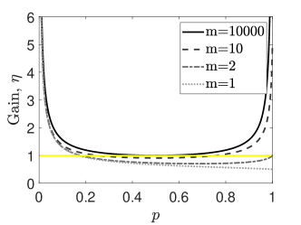
Note from Corollary 1 that when , the receiver can compute without recovering . It holds that
| (4) |
where the limit is the same as the gain for the DSBS model studied in [11], which tends to infinity as .
We illustrate the gain as a function of in Figure 1, indicating that may be substantially less than the joint entropy of the sources for this special class of source PMFs.
It has been shown in [12], [13] that via embedding the nonlinear function , where , in a sufficiently large prime , the decoder can reconstruct , and hence, compute with high probability. For instance, if , we can reconstruct from using a sum rate of .
Motivated by the notion of embedding in [12] and [13], we next devise an achievability scheme for computing , where the key idea is to compress the vector-wise embeddings of the sources vectors and via employing the linear structured encoding scheme of [11], in contrast to entry-wise embeddings that require a sum rate of (cf. [12] and [13]).
Proposition 2.
(Vector-wise embeddings followed by linear encoding for distributed computation of .) Given two sequences of vectors and , generated by two correlated memoryless sources, with entries from a field with , restricting the source mappings to be linear, the following sum rate is achievable via the Körner-Marton’s scheme to recover at the receiver with a small probability of error:
| (5) |
where for even, and for odd, respectively, and denotes a modulo- addition.
Proof.
The proof follows from noting that the receiver, upon receiving and , can reconstruct
where there is a unique for which .
For details, we refer the reader to Appendix -F. ∎
We next describe a hybrid encoding scheme. Note that can be rewritten as if is known. Exploiting Körner’s characteristic graphs [16] to enable nonlinear encoding of 111For a detailed description of characteristic graphs and their entropies, we refer the reader to [17, 18, 19]., the minimum compression rate of for computing given side information equals the conditional graph entropy of given , denoted by , as introduced by Orlitsky and Roche [15]. Via concatenating the structured coding scheme of Körner and Marton [11] to first compute and then the unstructured coding model of Orlitsky and Roche [15] to next determine , it is possible to achieve a sum rate . When , the required rate is , which is smaller than because [15].
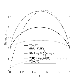
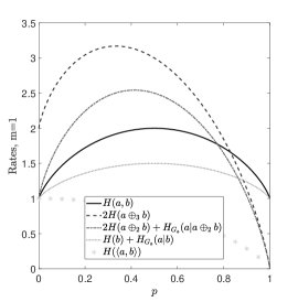
In Figure 2, we contrast the sum rate performance of Propositions 1-2 for distributed computing of of vectors with a small probability of error, with existing unstructured and structured coding schemes. In Figure 2-(Left), we use the PMF in Corollary 1 where , i.e., the pairs and represent DSBSs, each with a crossover probability . Note that the sum rates and perform poorly versus , and are not indicated. The sum rate converges to at low .
In Figure 2-(Middle), we use , and the pair is a DSBS with a crossover probability . At low , and converge to whereas performs poorly. For large , structured coding yields low rates ( and ).
In Figure 2-(Right), we use , and the pairs and are DSBSs, each with a crossover probability . The performance of is worse than and not shown. Similarly, is higher than , and is not indicated. For any given value, is always smaller than , and approaches for small and large .
II-B Distributed Computation of Symmetric Matrices
We next consider a generalization of Proposition 1 for distributed computing of inner products to distributed computing of a square symmetric matrix , given by the product , where , for and , and symmetry implies that for every .
Proposition 3.
(Computing symmetric matrices via distributed multiplication.) Given two sequences of random matrices and generated by two correlated memoryless -ary sources, respectively, where and , the achievable sum rate by the separate encoding of the sources for the receiver to recover the symmetric matrix with vanishing error is given as
| (6) |
where , , and are matrix variables.
Proof.
In the scheme of Proposition 3, similar to Proposition 1, the receiver may not recover and in their entirety, using , , and , hence rendering secure distributed compression of the sources feasible. To achieve information-theoretically secure distributed matrix multiplication, our future work includes exploiting the polynomial encoding scheme in [22] that incorporates random matrices, and the techniques in [23], [24].
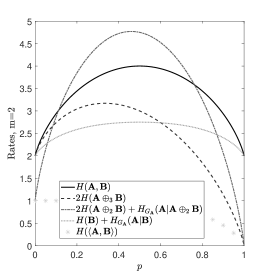
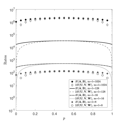
In Figure 3-(Left), we showcase the sum rates and versus (in log scale) for distributed computing of symmetric matrices for under assumptions222For , it is clear (from Appendix -G of Proposition 3) that the choices of , , and guarantee the recovery of without assumptions i)-ii).: i) , i.e., , and ii) . Because is symmetric, i) and ii) lead to
where and follow from assumptions i) and ii), respectively. These assumptions ensure a rate gain of that grows exponentially fast, as tends to .
We next state a necessary condition for successful recovery of , where , without recovering and . This result holds true for any symmetric .
Proposition 4.
Proof.
II-C Distributed Computation of Square Matrices
Recall that Proposition 3 does not capture non-symmetric matrix products. We here consider distributed computing of a square matrix , given by the product , where is not symmetric, and , for , and . The following proposition gives an achievable distributed encoding scheme of the sources and towards computing .
Proposition 5.
(Computing square matrices via distributed matrix multiplication.) Given two sequences of random matrices and generated by two correlated memoryless -ary sources, where , the following sum rate is achievable by the separate encoding of the sources for the receiver to recover a general square matrix with vanishing error:
| (8) |
where we use the shorthand notation for , where are matrix variables, is a length row vector of all ones, where with for .
Proof.
We refer the reader to Appendix -I. ∎
To demonstrate the performance of Proposition 5, we next consider a corollary, where , , and with .
Corollary 2.
Given and with entries for some , and that are i.i.d. across and the joint PMF of satisfies
The sum rate for distributed encoding of is given as
| (9) |
Exploiting Proposition 5 to compute , we can achieve
| (10) |
Proof.
We refer the reader to Appendix -J. ∎
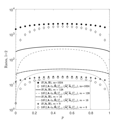
In Figure 3-(Right), we demonstrate the sum rate performance of Proposition 5 (in log scale) versus via contrasting the sum rates and (8) for the joint PMF model in Corollary 2, where we assume that . We observe that the rate gain grows exponentially fast, as tends to .
Discussion. We proposed structured coding techniques for nonlinear mappings of distributed sources in a -ary prime finite field to perform inner product-based matrix computation toward realizing distributed multiplication for special matrix classes, e.g., symmetric and square matrices, through imposing structural constraints on sources. Our future work includes the study of general matrix products, providing insights into the problems of distributed rank computation, trace computation, and low-rank matrix factorization, as well as the derivation of tighter achievability bounds for the distributed multiplication of general matrices and higher dimensional matrices or tensors.
Acknowledgment
The author gratefully acknowledges the constructive discussions with Prof. Arun Padakandla at EURECOM.
-D Proof of Proposition 1
The receiver aims to compute the inner product , with entries from a field of characteristic . Here, we focus on , and the generalization to is straightforward [14].
Encoding: Sources devise mappings and , respectively, defined below, to determine the binary-valued column vectors
| (11) | ||||
| (12) |
We denote by the length source vectors. The encoders of the sources and are defined by functions and , where and denote the ranges of and , respectively. The pair of functions is called an -coding scheme if there exists a function such that by letting
| (13) |
we have . Here, is the modulo-two sum of and , i.e., .
Our encoding scheme requires a well-known lemma of Elias [25], which showed that linear codes achieve the capacity of binary symmetric channels, and its adaption to the problem of computing the modulo-two sum of DSBSs in [11]. Using a simple generalization of this result to vector variables, for fixed and for sufficiently large , there exists a binary matrix , where and denote the modulo-two product of the matrix with the transpose of the binary vector sequences and , respectively, and a decoding function that satisfy
such that i) , and ii) . Hence, application of Elias’s lemma [25] and [11] yields that is an -coding scheme.
Decoding: Exploiting the achievability result of Körner-Marton [11], the sum rate needed for the receiver to recover the vector sequence with a vanishing error probability can be determined as [11]:
| (14) |
Using given in ii), the receiver can recover . However, lossless decoding of and is not guaranteed.
We next show that the sum rate in (14) is sufficient to recover . Using , the receiver computes
| (15) | |||||
where follows from .
-E Proof of Corollary 1
Employing the definitions of and in (11), (1) and [11], we can determine the sum rate needed for the receiver to recover in an asymptotic manner:
| (16) |
where follows from employing the relations and , and simplification using conditioning, follows from employing and , from the definition of , and from , where , such that , exploiting that , and . Finally, incorporating , we obtain .
The encoding rate for asymptotic lossless compression of and is given by the Slepian-Wolf theorem [10]:
| (17) |
where follows from using and , with , , and and having i.i.d. entries.
-F Proof of Proposition 2
Here, we provide a sketch of the proof. For binary sources, i.e., , it is easy to verify that
where for even, and for odd, respectively. Hence, the following sum rate is achievable:
| (18) |
When the data is generated by two correlated memoryless -ary sources for , it is possible to achieve a sum rate
where and for even and odd , respectively. Upon receiving and , the receiver can reconstruct
where there is a unique for which .
-G Proof of Proposition 3
Given two sequences of random matrices , the receiver aims to compute .
Encoding: Each source uses mappings and , to determine the respective matrices:
| (19) | ||||
| (20) |
Following the steps of Appendix -D, there exists an -coding scheme for a matrix , where , for decoding with a small probability of error.
Decoding: Exploiting the achievability result of Körner-Marton [11], the sum rate needed for the receiver to recover the matrix sequence with a vanishing error probability can be determined as [11]:
| (21) |
For , given a symmetric matrix , the following relation holds:
| (22) |
Using , the receiver computes
| (23) |
where the last equality follows from that is a symmetric matrix and it satisfies (22).
-H Proof of Proposition 4
We first show that the encoding scheme of Proposition 1 does not allow the recovery of by the receiver, i.e., , for .
The receiver can recover and with a small probability of error. The extra rate needed from the encoders for the receiver to determine is
where follows from using the definition of conditional entropy and that the receiver can compute from and , from , from and given , from , from employing the definition of conditional entropy, and holds with equality if the function is partially invertible, i.e., , e.g., when is the arithmetic sum or the modulo sum of the two vectors. Hence, the inequality in is strict for inferring from and .
We next prove the main result of the proposition. Given matrix variables such that is symmetric, letting , we first expand as
| (24) |
We next expand as
| (25) |
where it is easy to observe that .
Similarly, via exploiting , we can show that
| (26) |
where .
When , we have and , hence, the above condition is equivalent to
-I Proof of Proposition 5
Note that for , where . Following the steps in Appendix -D, the receiver can recover , and then compute the following matrix:
which is a symmetric matrix with unknowns and linearly independent equations for and . Hence, , for each , as well as can be recovered.
-J Proof of Corollary 2
The sum rate for distributed encoding of is given as
Exploiting Proposition 5 to compute , we can achieve
where the last step follows from using that
and evaluating the conditional entropy as
where follows from that can be recovered given the side information for and , and given , for . More specifically, the receiver can recover
| (27) |
Hence, using the side information and (27), the receiver can recover as follows:
Finally, step follows from exploiting that both variable and variable reside in .
References
- [1] G. Strang, Introduction to linear algebra. SIAM, 2022.
- [2] M. H. Mousavi, M. A. Maddah-Ali, and M. Mirmohseni, “Private inner product retrieval for distributed machine learning,” in Proc., IEEE Int. Symp. Inf. Theory (ISIT), Paris, France, Jul. 2019, pp. 355–359.
- [3] É. Bouscatié, G. Castagnos, and O. Sanders, “Pattern matching in encrypted stream from inner product encryption,” in Proc., IACR Int. Conf. Public-Key Cryptogr. Springer, May 2023, pp. 774–801.
- [4] H. Buhrman, R. Cleve, J. Watrous, and R. De Wolf, “Quantum fingerprinting,” Physical Review Letters, vol. 87, no. 16, p. 167902, Sep. 2001.
- [5] R. Tandon, Q. Lei, A. G. Dimakis, and N. Karampatziakis, “Gradient coding: Avoiding stragglers in distributed learning,” in International Conference on Machine Learning. PMLR, Jul. 2017, pp. 3368–3376.
- [6] Q. Yu, M. Maddah-Ali, and S. Avestimehr, “Polynomial codes: an optimal design for high-dimensional coded matrix multiplication,” in Proc., Advances in Neural Information Processing Systems, vol. 30, Long Beach, CA, Dec. 2017, pp. 4403––4413.
- [7] S. Dutta, M. Fahim, F. Haddadpour, H. Jeong, V. Cadambe, and P. Grover, “On the optimal recovery threshold of coded matrix multiplication,” IEEE Trans. Inf. Theory, vol. 66, no. 1, pp. 278–301, Jul. 2019.
- [8] M. Soleymani, H. Mahdavifar, and A. S. Avestimehr, “Analog lagrange coded computing,” IEEE J. Sel. Areas Inf. Theory, vol. 2, no. 1, pp. 283–295, Feb. 2021.
- [9] Q. Yu, S. Li, N. Raviv, S. M. M. Kalan, M. Soltanolkotabi, and S. A. Avestimehr, “Lagrange coded computing: Optimal design for resiliency, security, and privacy,” in Proc., Int. Conf. Artif. Intell. Stat. Naha, Okinawa, Japan: PMLR, Apr. 2019, pp. 1215–1225.
- [10] D. Slepian and J. K. Wolf, “Noiseless coding of correlated information sources,” IEEE Trans. Inf. Theory, vol. 19, no. 4, pp. 471–480, Jul. 1973.
- [11] J. Körner and K. Marton, “How to encode the modulo-two sum of binary sources (corresp.),” IEEE Trans. Inf. Theory, vol. 25, no. 2, pp. 219–221, Mar. 1979.
- [12] D. Krithivasan and S. S. Pradhan, “Distributed source coding using abelian group codes: A new achievable rate-distortion region,” IEEE Trans. Inf. Theory, vol. 57, no. 3, pp. 1495–1519, Feb. 2011.
- [13] S. S. Pradhan, A. Padakandla, F. Shirani et al., “An algebraic and probabilistic framework for network information theory,” Found. Trends Commun. Inf. Theory, vol. 18, no. 2, pp. 173–379, Dec. 2020.
- [14] T. Han and K. Kobayashi, “A dichotomy of functions F(X, Y) of correlated sources (X, Y),” IEEE Trans. Inf. Theory, vol. 33, no. 1, pp. 69–76, Jan. 1987.
- [15] A. Orlitsky and J. R. Roche, “Coding for computing,” IEEE Trans. Inf. Theory, vol. 47, no. 3, p. 903–917, Mar. 2001.
- [16] J. Körner, “Coding of an information source having ambiguous alphabet and the entropy of graphs,” in Proc., 6th Prague Conf. Inf. Theory, Prague, Czech Republic, Sep. 1973, pp. 411–425.
- [17] S. Feizi and M. Médard, “On network functional compression,” IEEE Trans. Inf. Theory, vol. 60, no. 9, pp. 5387–5401, Sep. 2014.
- [18] D. Malak, “Fractional graph coloring for functional compression with side information,” in Proc., IEEE Inf. Theory Wksh., Mumbai, India, Nov. 2022, pp. 750–755.
- [19] M. R. Deylam Salehi and D. Malak, “An achievable low complexity encoding scheme for coloring cyclic graphs,” in Proc., Annu. Allerton Conf. Commun. Control Comput., Monticello, IL, USA, Sep. 2023, pp. 1–8.
- [20] R. Ahlswede and T. Han, “On source coding with side information via a multiple-access channel and related problems in multi-user information theory,” IEEE Trans. Inf. Theory, vol. 29, no. 3, pp. 396–412, May 1983.
- [21] C. Nair and Y. N. Wang, “On optimal weighted-sum rates for the modulo sum problem,” in Proc., IEEE Int. Symp. Inf. Theory, Jun. 2020, pp. 2416–2420.
- [22] W.-T. Chang and R. Tandon, “On the capacity of secure distributed matrix multiplication,” in Proc., IEEE Global Commun. Conf., Abu Dhabi, UAE, Dec. 2018, pp. 1–6.
- [23] Z. Jia and S. A. Jafar, “On the capacity of secure distributed batch matrix multiplication,” IEEE Trans. Inf. Theory, vol. 67, no. 11, pp. 7420–7437, Sep. 2021.
- [24] Y. Zhao and H. Sun, “Expand-and-randomize: An algebraic approach to secure computation,” Entropy, vol. 23, no. 11, p. 1461, Nov. 2021.
- [25] R. G. Gallager, Information theory and reliable communication. Wiley: New York, Jan. 1968, vol. 588.