Weakening the effect of boundaries: ‘diffusion-free’ boundary conditions as a ‘do least harm’ alternative to Neumann

Abstract

In this note, we discuss a poorly known alternative boundary condition to the usual Neumann or ‘stress-free’ boundary condition typically used to weaken boundary layers when diffusion is present but very small. These ‘diffusion-free’ boundary conditions were first developed (as far as the authors know) in 1995 (Sureshkumar & Beris J. Non-Newtonian Fluid Mech. 60, 53-80, 1995) in viscoelastic flow modelling but are worthy of general consideration in other research areas. To illustrate their use, we solve two simple ODE problems and then treat a PDE problem - the inertial wave eigenvalue problem in a rotating cylinder, a sphere and spherical shell for small but non-zero Ekman number $E$. Where inviscid inertial waves exist (cylinder and sphere), the viscous flows in the Ekman boundary layer are $O(E^{1/2})$ weaker than for the corresponding stress-free layer and fully $O(E)$ weaker than in a non-slip layer. This reduction could allow precious numerical resources to focus on other areas of the flow and thereby make smaller, more realistic values of diffusion accessible to simulations.

1 Introduction

In many flow situations of interest, diffusion of a given physical quantity may be so small relative to other effects that it would appear safely neglectable. The well-known caveat to this is the presence of boundaries where small scales can make diffusion a leading order effect to accommodate the boundary conditions. The situation can be even more complicated if these boundary layers also generate internal shear layers in which diffusion plays an enhanced role in the bulk (e.g. the inertial wave problem to be discussed below). The strategy almost always is either to take the smallest diffusion coefficient possible which still allows accurate solutions to be computed (even though this may be orders of magnitude bigger than the actual value) and/or the boundary conditions are adjusted to weaken the boundary layers and possibly internal layers which result. In the case of high Reynolds number flows (or low Ekman numbers) where momentum diffusion is small, the latter is invariably achieved by adopting ‘stress-free’ boundary conditions instead of the usual ‘non-slip’ conditions of the flow at a solid boundary (e.g. Vidal & Cebron, 2023). This, however, can create its own problems in that stress-free boundary conditions prevent any angular momentum transfer through viscous stresses in rotating systems (Vidal & Cebron, 2023).

The purpose of this short note is to describe a further option - hereafter referred to as ‘diffusion-free’ boundary conditions - for mitigating the effects of diffusion and to demonstrate that they produce an even weaker viscous boundary layer correction than ‘stress-free’ or Neumann conditions. In the interests of clarity, we specialise below to the vanishing viscosity situation although it should be clear that what follows is perfectly general for handling the diffusion of any physical quantity, e.g. a scalar like density, another vector such as a magnetic field or even a tensor like the conformation tensor in viscoelastic fluids. In fact, it is within the viscoelastic flow community that the new boundary condition was (as far as the authors are aware) first used (Sureshkumar & Beris, 1995; Sureshkumar et al., 1997). Here, the correct boundary condition on the conformation tensor, which describes an ensemble-averaged configuration of the polymers, is unclear and so those authors decided to simply turn the diffusion off at the boundary. This meant that the diffusion-free equation was imposed at the wall as the required extra boundary conditions or, equivalently, for a $C^{2}$ solution, the (tensorial) Laplacian of the conformation tensor had to vanish. Carrying this over to the flow velocity, the idea is to augment the usual (inviscid) no-penetration normal condition with the extra conditions that the tangential components of the inviscid equation hold there. Again for a sufficiently smooth velocity field, this is equivalent to imposing that the tangential components of the viscous (vectorial) Laplacian term vanish. Imposing that the second derivative must vanish when solving a second order equation appears paradoxical. But, in fact, all this does for a smooth solution is impose that the ‘rest’ of the equation (comprising of first and zeroth derivative terms) vanishes at the boundary so the diffusion-free boundary condition is equivalent to a generalised Robin condition (‘generalised’ as this condition can be a nonlinear relation between zeroth and first derivatives).

Boundary conditions which include the second derivative for a second order equation are not new. They have been been studied since the 1950s (Feller, 1952; Ventcel, 1959) in the mathematical analysis literature and variously go under the names of ‘Ventcel’ (e.g. Buffe (2017)), ‘Ventsell’ (e.g. Hinz et al. (2018)) or ‘Wentzell’ (e.g. Denk et al. (2021)) boundary conditions. The novelty introduced by Sureshkumar & Beris (1995) was to implicitly use a special form of them when artificially smoothening a differential equation.

We first illustrate the diffusion-free boundary condition for a couple of simple ODE problems and then to demonstrate how it works for a realistic PDE case. The inertial wave problem is chosen for the latter as: a) it is relevant for rapidly rotating systems such as the Earth’s core (Vidal & Cebron, 2023) where the exact tangential boundary conditions are unclear; b) it has some challenging viscous features to resolve in the form of internal shear layers (McEwan, 1970); c) it is still an area of active research (e.g. He et al., 2022, 2023; Le Dizes, 2023); and finally d) it is an opportunity to update some 30-year-old work by one of the authors (Kerswell & Barenghi, 1995, hereafter KB95).

2 Model Problem 1: Nonlinear Robin condition

We first start by considering the simple, albeit nonlinear, ODE problem

$$y^{\prime}=-y^{2}$$ (1)

over $x\in[0,1]$ ($y^{\prime}:=dy/dx$) with boundary condition $y(0)=1$. This has the solution $y=1/(1+x)$. Now imagine that there is actually very weak diffusion in the system and really the equation is

$$y^{\prime}=-y^{2}+\varepsilon y{{}^{\prime\prime}}$$ (2)

with the diffusion coefficient $\varepsilon\ll 1$. The question then arises as to what extra boundary condition to impose at $x=1$ because the problem is now second order. If known, the physically-relevant condition is the natural one, of course, but sometimes this is unclear or there is a need to minimise the effect of the boundary to examine its influence or perhaps reduce the numerical resolution needed to capture the interior solution. Then there is interest in selecting the boundary condition which does ’least harm’ to the interior solution. To explore this, we now examine the effect of imposing: (i) a Dirichlet condition $y(1)=0$; (ii) a Neumann condition $y^{\prime}(1)=0$; or (iii) the new ‘diffusion-free’ condition $y^{\prime}(1)=-y(1)^{2}$ which is equivalent to $y^{\prime\prime}(1)=0$ for a smooth solution.

The three problems can be straightforwardly solved using matched asymptotic expansions to give the leading composite solutions:

$$\begin{array}[]{lll}(i)&y=\displaystyle{\frac{1}{1+x}-\frac{1}{2}e^{-(1-x)/\varepsilon}}&{\rm Dirichlet},\\ &&\\ (ii)&y=\displaystyle{\frac{1}{1+x}+\frac{1}{4}\varepsilon e^{-(1-x)/\varepsilon}}&{\rm Neumann},\\ &&\\ (iii)&y=\displaystyle{\frac{1}{1+x}-\frac{1}{4}\varepsilon^{2}e^{-(1-x)/\varepsilon}}&{\rm Diffusion\!\!-\!\!free}.\end{array}$$ (3)

The first term on the RHS represents the leading ‘outer’ solution (with the next correction being $O(\varepsilon)$) and each second term is the leading ‘inner’ boundary layer correction. The take-home message here is that this is $O(1)$ for the Dirichlet condition, $O(\varepsilon)$ for the Neumann condition and $O(\varepsilon^{2})$ for the diffusion-free condition which therefore creates the weakest boundary layer correction. It’s worth remarking also that the actual condition imposed is $y^{\prime}(1)=-y(1)^{2}$ which is not the usual (linear) Robin condition due to the nonlinearity in $y$ but a suitable generalisation i.e. a nonlinear relationship between $y$ and $y^{\prime}$ which is imposed at $x=1$.

3 Model Problem 2: Interior smoothening

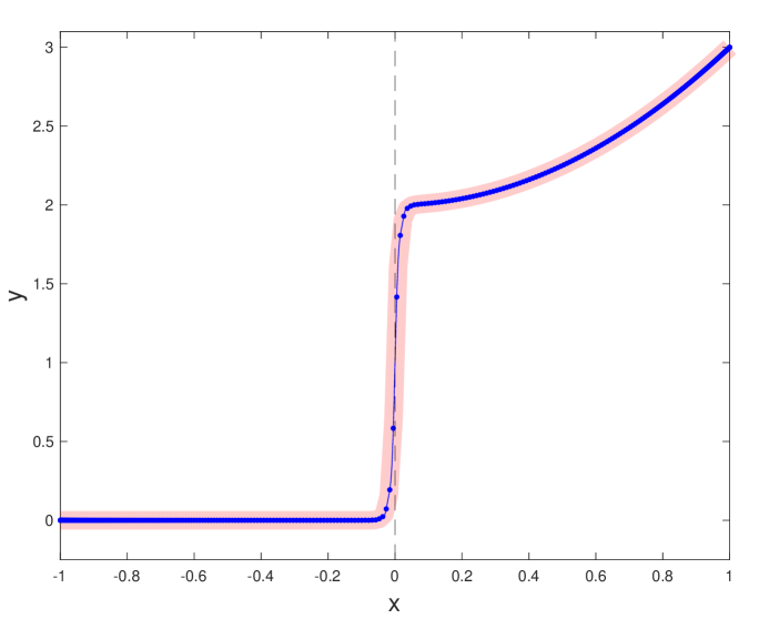
The second ODE problem we consider is

$$y=(2+x^{2})H(x)\,:=\left\{\begin{array}[]{lr}2+x^{2}&\qquad x\geq 0\\ 0&\qquad x<0\end{array}\right.$$ (4)

for $x\in[-1,1]$ and $H(x)$ is the Heaviside function. This has a discontinuity at $x=0$ such as could be present in a hyperbolic system and non-zero first and second derivatives at one boundary for reasons which will become clear immediately below. To smooth the solution (e.g. to numerically estimate it), diffusion could be added as follows

$$y=(2+x^{2})H(x)+\varepsilon^{2}y^{\prime\prime}$$ (5)

to target the discontinuity hopefully leaving the rest of the solution largely unchanged (the diffusion coefficient $\varepsilon^{2}$ controls the amount of smoothening). This makes the problem second order requiring two new boundary conditions. We now show again that the effect of the diffusion-free boundary conditions will be less disruptive on the original solution than adopting Neumann (‘stress-free’) conditions.

Figure 1: Left: The difference between the stress-free solution $y_{s}$ and the diffusion-free solution $y_{0}$ is plotted on a log scale in red together with the corresponding difference between the diffusion-free boundary condition solution (9), $y_{d}$, and $y_{0}$ (in blue) for $\varepsilon=0.01$ near $x=1$. This plot demonstrates that the stress-free solution produces a larger deviation at the boundary in $y$: both have an unavoidable interior deviation of $O(\varepsilon^{2})$ due to the change in the ODE and an $O(1)$ deviation at the discontinuity where $x=O(\varepsilon)$. Right: a numerical solution for (9) shown as the thin blue line again for $\varepsilon=0.01$ using a spectral method with 300 Chebyshev polynomials (blue dots indicate the collocation points used; it is expected that $O(1/\varepsilon)$ polynomials are needed due to sparse collocation point spacing at the middle of the $[-1,1]$ range). The thick transparent red line is the analytic expression $y_{d}(x)$ given in (9). Note that the same result is obtained imposing the equivalent boundary condition that $y^{\prime\prime}=0$ at $x=\pm 1$.

3.1 Neumann boundary conditions

Neumann (stress-free) boundary conditions are

$$y^{\prime}(-1)=0\quad\&\quad y^{\prime}(1)=0$$ (6)

which are often viewed as minimally disruptive. This choice leads to the leading asymptotic solution

$$y_{s}\sim\left\{\begin{array}[]{cr}\displaystyle{2(1+\varepsilon^{2})e^{-1/\varepsilon}\cosh\left(\frac{1+x}{\varepsilon}\right)}&x<0,\\ \displaystyle{2+x^{2}+2\varepsilon^{2}+2\varepsilon\sinh\left(\frac{1-x}{\varepsilon}\right)-\biggl{[}\,2\varepsilon+2(1+\varepsilon^{2})e^{-1/\varepsilon}\,\biggr{]}\cosh\left(\frac{1-x}{\varepsilon}\right)}&x\geq 0.\end{array}\right.$$ (7)

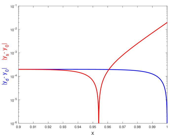
There are then 3 distinct scalings for how this solution differs from the diffusion-free solution $y_{0}$ of (4): for $x=0(\varepsilon)$, $y_{s}-y_{0}=O(1)$, for $1-x=O(\varepsilon)$, $y_{s}-y_{0}=O(\varepsilon)$ to fix up the boundary condition, and otherwise $y_{s}-y_{0}=O(\varepsilon^{2})$ - see Figure 1.

3.2 Diffusion-free boundary conditions

We now impose ‘diffusion-free’ boundary conditions which are just

$$y(-1)=(2+x^{2})H(x)|_{x=-1}=0\quad\&\quad y(1)=(2+x^{2})H(x)|_{x=1}=3$$ (8)

The leading asymptotic solution is then

$$y_{d}\sim\left\{\begin{array}[]{cr}\displaystyle{2(1+\varepsilon^{2})e^{-1/\varepsilon}\sinh\left(\frac{1+x}{\varepsilon}\right)}&x<0,\\ \displaystyle{2+x^{2}+2\varepsilon^{2}\biggl{[}\,1-\cosh\left(\frac{1-x}{\varepsilon}\right)\,\biggr{]}+\biggl{[}\,2\varepsilon^{2}-2(1+\varepsilon^{2})e^{-1/\varepsilon}\,\biggr{]}\sinh\left(\frac{1-x}{\varepsilon}\right)}&x\geq 0.\end{array}\right.$$ (9)

There are now only 2 distinct scalings for how this solution differs from the solution $y_{0}$ of (4): for $x=O(\varepsilon)$, $y_{d}-y_{0}=O(1)$ otherwise $y_{s}-y_{0}=O(\varepsilon^{2})$ - see Figure 1. The key point here is that the order of the correction does not change at the boundary in contrast to the Neumann case where the correction grows to $O(\varepsilon)$. In fact, in this model problem the correction goes to precisely zero there because the $\varepsilon=0$ problem has a well defined boundary value. Hence, again, diffusion-free conditions are better ‘do least harm’ conditions than Neumann.

The problem (5) & (8) can also be solved numerically using a standard Chebyshev expansion and shows no issues - see Figure 1(right). It’s worth remarking that the same solution is obtained (up to discretization errors) if the boundary conditions $y^{\prime\prime}(\pm 1)=0$ are used instead. These are equivalent for a smooth solution of course.

4 Inertial wave problem in a cylinder

We now switch our attention to a more serious PDE example. The linearised equations for describing small motions of a viscous, incompressible fluid away from uniform rotation are

$$\frac{\partial\mathbf{u}}{\partial t}+2\mathbf{\hat{z}}\times\mathbf{u}+\mbox{\boldmath$\nabla$}p=E\nabla^{2}\mathbf{u},$$ (10)

$$\mbox{\boldmath$\nabla$}.\mathbf{u}=0,$$ (11)

in the rotating frame. This is a core problem in rotating flows with appropriately more complicated analogues when further physics is present (e.g. stratification and/or magnetic fields). It also displays a number of fascinating viscous features typified by boundary layer breakdowns which give rise to internal shear layers and a host of different viscous lengthscales (e.g. see figure 4 of He et al. (2022)). The basic rotation rate $\Omega$ and cylindrical radius $S$ have been used to non-dimensionalise the system, with the Ekman number $E=\nu/\Omega S^{2}$ appearing as the non-dimensionalization of the kinematic viscosity $\nu$.

The inviscid limit, in which $E$ is set to zero and only a no-normal velocity boundary condition needs be applied, gives rise to the well known inertial wave problem, where wave solutions

$$[\mathbf{u},p]=[u(s,z),v(s,z),w(s,z),\Phi(s,z)]e^{i(m\phi+\lambda t)},$$

may be sought (e.g. see Greenspan (1968); Zhang & Liao (2017)), and $(s,\phi,z)$ are cylindrical coordinates). The reduction of the problem to one for only the pressure realises the Poincaré (1910) equation

$$\frac{1}{s}\frac{\partial}{\partial s}s\frac{\partial\Phi}{\partial s}-\frac{m^{2}}{s^{2}}\Phi+\left(1-\frac{4}{\lambda^{2}}\right)\frac{\partial^{2}\Phi}{\partial z^{2}}=0$$ (12)

to be solved subject to the boundary conditions

$$\frac{\partial\Phi}{\partial s}+\frac{2m}{\lambda s}\Phi = 0\quad{\rm on}\,s=1,$$

$$\frac{\partial\Phi}{\partial z} = 0\quad{\rm on}\,z=0,\,d.$$

For the cylinder problem, Kelvin (1880) first wrote down the separable solutions

$$\mathbf{u}_{mnl}=\frac{e^{i(m\phi+\lambda t)}}{2(4-\lambda^{2})}\left[\begin{array}[]{c}i\{(\lambda+2)J_{m-1}(ks)-(\lambda-2)J_{m+1}(ks)\}\cos(l\pi z/d)\\ -\{(\lambda+2)J_{m-1}(ks)+(\lambda-2)J_{m+1}(ks)\}\cos(l\pi z/d)\\ 2i\lambda kd(\pi l)^{-1}J_{m}(ks)\sin(l\pi z/d)\end{array}\right],$$ (13)

$$p=-\frac{1}{k}J_{m}(ks)\cos(l\pi z/d)e^{i(m\phi+\lambda t)},$$ (14)

where

$$\lambda=\frac{\pm 2}{\sqrt{1+k^{2}d^{2}/(\pi l)^{2}}},$$

and $k$ is a solution, indexed by $n$ such that $0\,<\,k_{n=1}\,<\,k_{n=2}\ldots$, of

$$s\frac{d}{ds}J_{m}(ks)+\frac{2m}{\lambda}J_{m}(ks)=0|_{s=1}.$$

Three numbers, $l$, $n\in{\mathbb{N}}$, and $m\in{\mathbb{Z}}$, are sufficient to specify the inertial mode and in particular the frequency $\lambda=\lambda_{lmn}$. These indices correspond roughly with the number of nodes axially, radially, and azimuthally respectively in the pressure eigenfunction. As in KB95 and Kerswell (1999), we focus here on the inertial mode with $m=n=l=1$ and $d=1.9898$ (the quoted value in KB95) with inertial velocity field $\mathbf{u}_{0}$ and real frequency $\lambda_{0}=1.000007648337\approx 1$. The subscript is to indicate that these are the $E=0$ quantities compared to those, $\mathbf{u}_{E}$ and $\lambda_{E}$, for $E\neq 0$. The viscous correction is then defined as $\mathbf{u}_{c}:=\mathbf{u}_{E}-\mathbf{u}_{0}$. Reinstating viscosity requires 2 extra (tangential) boundary conditions to supplement to no-penetration (normal) condition.

4.1 Non-slip boundary conditions

If the container walls are rigid then non-slip boundary conditions are required which is the usual case discussed in text books (e.g. §2.5 in Greenspan (1968)). If $\mathbf{u}_{0}(\mathbf{x})e^{i\lambda t}$ is the solution to the inertial wave problem (12) with $\lambda$ a real frequency in the interval $[-2,2]$ for $E=0$, then the leading viscous correction for $E\neq 0$ is the $O(E^{0})$ boundary velocity ${\mathbf{\tilde{u}}}_{0}(\mathbf{x},t)$ forced by the non-slip condition

$$\mathbf{u}_{0}+{\mathbf{\tilde{u}}}_{0}={\bf 0}|_{\partial V}.$$ (15)

(hereafter $\mathbf{\tilde{\,\,}}$ indicates a boundary layer flow). This decays into the interior from the boundary over an Ekman boundary of thickness $E^{1/2}$ but drives an $O(E^{1/2})$ viscous flow $\mathbf{u}_{1}(\mathbf{x},t)$ in the interior by ‘Ekman pumping’ (equation 2.6.13 in Greenspan (1968)). These flows mean that $\lambda$ becomes complex with a viscous decay rate $\lambda_{i}:=\Im m(\lambda)=O(E^{1/2})\,>\,0$. There are also shear layers spawned by the corners of the cylinder (e.g. McEwan (1970) and figures 2-4 below) but these appear unimportant for the leading decay rate calculation (§2.9 in Greenspan (1968)).

4.2 Stress-free boundary conditions

For other situations, the boundary may be stress-free (e.g. for a gaseous planet) or this choice is assumed to make the viscous correction at the boundary as weak as possible (e.g. Lin & Ogilvie (2021); Vidal & Cebron (2023)). Then the leading viscous correction is $E^{1/2}{\mathbf{\tilde{u}}}_{1}(\mathbf{x},t)$ in a boundary layer of thickness $E^{1/2}$ such that, at, for example, the cylinder sidewall,

$$s\frac{\partial}{\partial s}\biggl{(}\frac{v_{0}}{s}\biggr{)}-\frac{\partial\tilde{v}_{1}}{\partial\xi}=0\biggl{|}_{s=1}\biggr{.}\quad\&\quad\frac{\partial w_{0}}{\partial s}-\frac{\partial\tilde{w}_{1}}{\partial\xi}=0\biggl{|}_{s=1}\biggr{.}$$ (16)

where $\xi:=(1-s)/E^{1/2}$ is the rescaled normal coordinate. The corrective viscous bulk flow (as opposed to localised shear layers) is then $O(E)$ driven by the subsequent $O(E)$ Ekman pumping at the boundaries and the bulk viscous term also of $O(E)$. As a result the viscous decay rate is much smaller - $\lambda_{i}:=O(E)\,>\,0$.

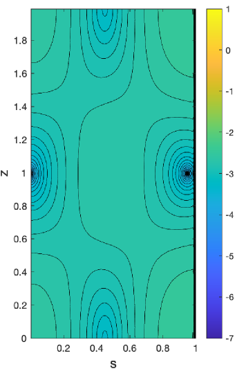
Unfortunately, for our purposes here, the cylinder has a singular feature for these boundary conditions: the inertial mode automatically satisfies stress-free conditions on the top and bottom boundaries, i.e. $\partial u_{0}/\partial z=\partial v_{0}/\partial z=0$ at $z=0$ and $z=d$ already. Hence a viscous boundary layer only forms on the side wall and in particular no internal shear layers are formed by the corner region where the horizontal boundaries meet the sidewall which is an exceptional response. - e.g. a calculation in more geophysically-interesting sphere or spherical shell does have shear layers (e.g. Lin & Ogilvie (2021); Vidal & Cebron (2023) and the next section). As a result, for stress-free boundary conditions, the calculation for the viscous decay rate $\lambda_{i}$ in a cylinder is just 1D - the variation in $z$ can be separated off - and so very small Ekman numbers can be reached easily (see Table 1).

4.3 Diffusion-free boundary conditions

Diffusion-free boundary conditions are

$$i\lambda u-2v+\frac{\partial p}{\partial s}=0,\quad i\lambda v+2u+\frac{imp}{s}=0\quad\&\quad w=0$$ (17)

on the top ($z=d$) and bottom ($z=0$) and

$$u=0,\quad i\lambda v+2u+\frac{imp}{s}=0\quad\&\quad i\lambda w+\frac{\partial p}{\partial z}=0$$ (18)

on the sides ($s=1$) of the cylinder. For a $C^{2}$ solution this is equivalent to setting the tangential components of the vectorial Laplacian to zero. That is, the conditions

$$u=0,$$

$$\mbox{\boldmath$\hat{\phi}$}.\nabla^{2}\mathbf{u}=\frac{\partial^{2}v}{\partial s^{2}}+\frac{1}{s}\frac{\partial v}{\partial s}-\frac{m^{2}+1}{s^{2}}v+\frac{\partial^{2}v}{\partial z^{2}}+\frac{2imu}{s^{2}}=0,$$

$$\mathbf{\hat{z}}.\nabla^{2}\mathbf{u}=\frac{\partial^{2}w}{\partial s^{2}}+\frac{1}{s}\frac{\partial w}{\partial s}-\frac{m^{2}}{s^{2}}w+\frac{\partial^{2}w}{\partial z^{2}}=0$$ (19)

imposed at $s=1$ are equivalent to those in (18) having the same complex frequencies $\lambda(E)$ as eigenvalues (not shown but verified).

4.4 Scalings

The inviscid inertial wave satisfies all the diffusion-free boundary conditions. However the $O(E)$ bulk viscous term drives a primary $O(E)$ interior flow, $E\mathbf{u}_{2}(\mathbf{x},t)$, which does not, leading to an $O(E)$ error in the diffusion-free boundary conditions (with no boundary-normal derivatives). These can be fixed up by a very weak $O(E)$ boundary correction flow, $E{\mathbf{\tilde{u}}}_{2}(\mathbf{x},t)$. The associated Ekman pumping drives a secondary bulk flow at $O(E^{3/2})$. Hence the corrective viscous flow is $O(E)$ in both the bulk and the Ekman boundary layer. In contrast, the secondary flow is $O(E)$ in the bulk and a larger $O(E^{1/2})$ in the boundary layer for stress-free boundary conditions. For non-slip conditions, the secondary flow is $O(E^{1/2})$ in the bulk and $O(1)$ in the boundary layer.

4.5 Numerical Implementation

We now demonstrate the scaling predictions discussed above using numerical calculations over a range of small but finite $E$. As in KB95, we exploit the symmetries of the inertial waves by only solving the eigenvalue problem (10)-(11) in the upper ‘quadrant’ $(s,z)\in[0,1]\times[d/2,d]$ of an extended cylinder $(s,z)\in[-1,1]\times[0,d]$. If $m$ (the azimuthal wavenumber) is even (odd), then $(w,p)$ are even (odd) and $(u,v)$ are odd (even) functions of $s$. Likewise about the cylindrical equator $z=d/2$, if $l$ is even (odd), then $(u,v,p)$ are even (odd) and $w$ is odd (even) functions of $z^{*}:=2z/d-1$. Hence, for the situation of interest here, $m=l=1$, the appropriate spectral expansions used are

$$(u,v)(s,z)=\sum^{N}_{i=1}\sum_{j=1}^{N}(u_{ij},v_{ij})T_{2i-2}(s)T_{2j-1}(z^{*}),$$ (20)

$$w(s,z)=\sum^{N}_{i=1}\sum_{j=1}^{N}w_{ij}T_{2i-1}(s)T_{2j-2}(z^{*}),\qquad p(s,z)=\sum^{N}_{i=0}\sum_{j=0}^{N}p_{ij}T_{2i-1}(s)T_{2j-1}(z^{*})$$ (21)

where $T_{n}(x):=\cos(n\cos^{-1}x)$ is the $n^{th}$ Chebyshev polynomial. The equations were collocated over the positive zeros of $T_{2N}$ in $s$ and $z^{*}$ (the expansion lengths in $r$ and $z$ are taken equal for simplicity). Inverse iteration was then used to find the relevant (complex) eigenvalue and eigenfunction as the inviscid real frequency $\lambda_{0}$ provides a good guess. KB95 talk about a maximal (given the 300 MBytes available) $N=35$ full eigenvalue solve taking 3 days on a Sun SparcCenter 2000 (the University of Newcastle’s largest computer in 1995). The equivalent today takes 9.4 mins on an Apple M1 laptop even using Matlab instead of the Fortran 77 of KB95. Employing inverse iteration to just focus on the eigenvalue of interest brings that down to just 18 seconds.

Table 1: Decay rates $\lambda_{i}$ at various $E$ and different boundary conditions. Non-slip and diffusion-free boundary conditions use up to $N=110$ to check convergence. The stress-free case reduces to a 1D problem and resolution can go much higher: $N=6,000$ and $10,000$ give $\lambda=1.0000076483366+i9.469658E$ for $E=10^{-10}$. Removing the top and bottom boundary conditions for the diffusion-free case gives the starred decay rates on the far right which shows convergence to the interior dissipation rate value of $9.97105E$ indicating that the boundary layer contribution is higher order.

$E$		KB95		non-slip		stress-free		diffusion-free
		$\lambda_{i}/\sqrt{E}$		$\lambda_{i}/\sqrt{E}$		$\lambda_{i}/E$		$\lambda_{i}/E$
$10^{-4}$		$1.5665$		$1.5665$		$9.4362$		$9.831$
$10^{-5}$		$1.4834$		$1.4859$		$9.4591$		$9.927$
$10^{-6}$				$1.4619$		$9.4663$		$9.957$  $9.9647*$
$3\times 10^{-7}$				$1.4571$				$9.963$
$10^{-7}$						$9.4686$		$9.9689^{*}$
$10^{-8}$						$9.4694$		$9.9703^{*}$
$10^{-9}$						$9.4696$		$9.9707^{*}$
$10^{-10}$						$9.4697$		$9.9708^{*}$
$10^{-11}$								$9.9709^{*}$
		$\underbrace{\hskip 92.47145pt}_{E\,\rightarrow\,0}$				$\underbrace{\hskip 135.15059pt}_{\text{interior dissipation only}}$
Wedemeyer		$1.732$				$9.97105$
Kudlick		$1.451$

Table 2: Convergence of decay rate $\lambda_{i}/\sqrt{E}$ estimates with varying $N$ for non-slip boundary conditions ($N=110$ is the largest resolution that runs on a 192GB memory machine).

$N$		$E=10^{-4}$		$E=10^{-5}$		$E=10^{-6}$		$E=3\times 10^{-7}$
30		$1.5664732$		$1.4861012$
40		$1.5665071$		$1.4870688$
50		$1.5665072$		$1.4866554$		$1.4396532$
60		$1.5665072$		$1.4865893$		$1.4684427$		$1.3328341$
70		$1.5665072$		$1.4865937$		$1.4623715$		$1.4502321$
80				$1.4865936$		$1.4622908$		$1.4639174$
90				$1.4865936$		$1.4619161$		$1.4581648$
100						$1.4618646$		$1.4571169$
110						$1.4618879$		$1.4571179$

Figure 2: Plots of the viscous corrective field for different boundary conditions at $E=10^{-4}$: non-slip (left) $\log_{10}|\mathbf{u}_{c}|$ plotted with $\max|\mathbf{u}_{c}|=4.24$, stress-fress (middle) $\log_{10}|\mathbf{u}_{c}|/\sqrt{E}$ plotted with $\max|\mathbf{u}_{c}|=3.03\sqrt{E}$ and diffusion-free conditions (right) $\log_{10}|\mathbf{u}_{c}|/E$ with $\max|\mathbf{u}_{c}|=44.56E$. This and figures 3 and 4 show how the viscous corrective flows scale with $E$ for the various boundary conditions.

4.6 Decay rate $\lambda_{i}$ and Eigenfunctions

To identify the viscous corrective flow to the inviscid inertial wave $\mathbf{u}_{111}$ - see (13) - due to $E\neq 0$, we use the well-known orthogonality property of inertial waves (§2.7 Greenspan (1968)) to renormalise the viscous eigenfunction to have exactly the inertial wave field $\mathbf{u}_{111}$ and then subtract it -

$$\mathbf{u}_{c}:=\biggl{[}\frac{\int_{V}\mathbf{u}^{*}_{111}.\mathbf{u}_{111}\,{\bf d}^{3}\mathbf{x}}{\int_{V}\mathbf{u}^{*}_{111}.\mathbf{u}_{E}\,{\bf d}^{3}\mathbf{x}}\biggr{]}\mathbf{u}_{E}-\mathbf{u}_{111}.$$ (22)

This definition means that $\mathbf{u}_{c}$ is orthogonal to $\mathbf{u}_{111}$ and is normalised to be the viscous correction to the field $\mathbf{u}_{111}$ as defined in (13)

Table 1 collects all the decay rate results across the 3 different boundary conditions mentioned above. Only the non-slip case was considered in KB95 and the results there are confirmed for $E=10^{-4}$ and now properly converged for $10^{-5}$. Treating even smaller $E$ suggests that Kudlick’s formula for the decay rate is to be preferred to Wedemeyer’s: see KB95 for context. Table 2 shows how the non-slip results converge. The $N=30$ result for $E=10^{-5}$ is misleadingly good compared to KB95. In fact $N=35$ gives $\lambda_{i}=1.4913$ before convergence really starts at $N=40$.

Figure 3: Plots of the viscous corrective field for different boundary conditions at $E=10^{-5}$: non-slip (left) $\log_{10}|\mathbf{u}_{c}|$ plotted with $\max|\mathbf{u}_{c}|=4.24$, stress-fress (middle) $\log_{10}|\mathbf{u}_{c}|/\sqrt{E}$ plotted with $\max|\mathbf{u}_{c}|=3.00\sqrt{E}$ and diffusion-free conditions (right) $\log_{10}|\mathbf{u}_{c}|/E$ with $\max|\mathbf{u}_{c}|=43.47E$. This and figures 2 and 4 show how the viscous corrective flows scale with $E$ for the various boundary conditions.

Figure 4: Plots of the viscous corrective field for different boundary conditions at $E=10^{-6}$: non-slip (left) $\log_{10}|\mathbf{u}_{c}|$ plotted with $\max|\mathbf{u}_{c}|=4.24$, stress-fress (middle) $\log_{10}|\mathbf{u}_{c}|/\sqrt{E}$ plotted with $\max|\mathbf{u}_{c}|=2.99\sqrt{E}$ and diffusion-free conditions (right) $\log_{10}|\mathbf{u}_{c}|/E$ with $\max|\mathbf{u}_{c}|=42.35E$. This and figures 2 and 3 show how the viscous corrective flows scale with $E$ for the various boundary conditions.

The contribution to the decay rate from the interior can be estimated as $(k^{2}+\alpha^{2})E$ (Kerswell (1999)) and with $\lambda^{2}=4/(1+k^{2}/\alpha^{2})$ is just $4\alpha^{2}E/\lambda^{2}=9.97104976E$. The diffusion-free decay rate is well approximated by

$$\lambda_{i}=9.97105E-14E^{3/2}+O(E^{2})$$ (23)

indicating that the boundary layer contribution is $O(E^{1/2})$ smaller than the interior’s (this is clearer for the 1D case where the top and bottom boundaries are made stress-free - see the starred entries in Table 1 which can be computed to much smaller $E$). This is in contrast to the stress-free case where the decay rate does not converge to the interior’s contribution as $E\rightarrow 0$ - see Table 1 - indicating that the boundary layer contribution is at the same order as the interior’s. Hence the diffusion-free boundary condition again is less disruptive than the stress-free (Neumann) condition.

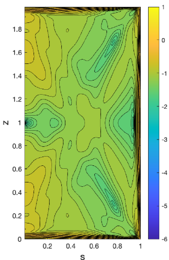
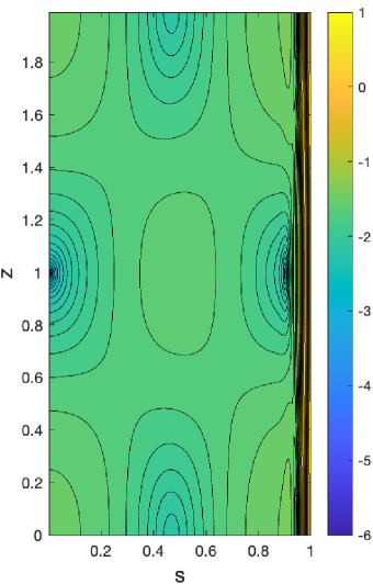
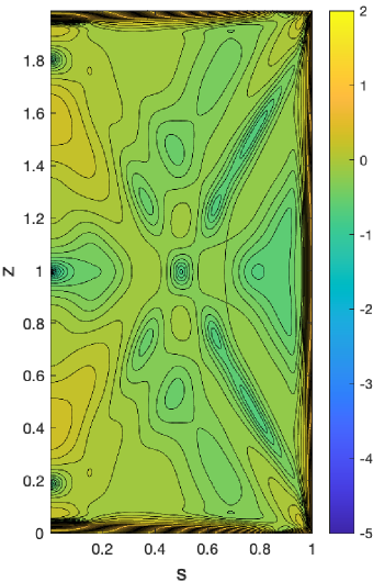
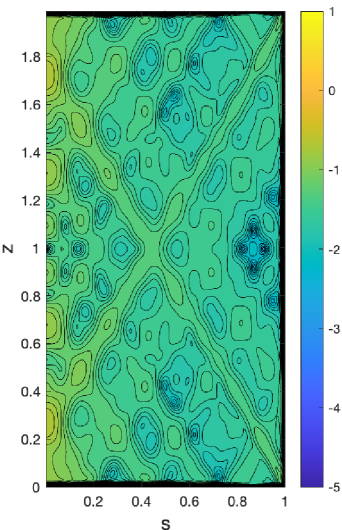
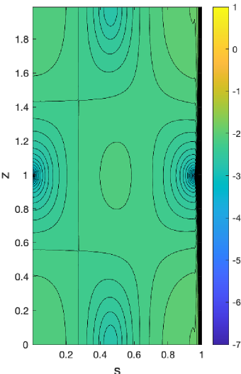
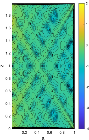
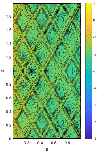
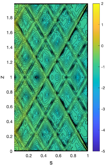
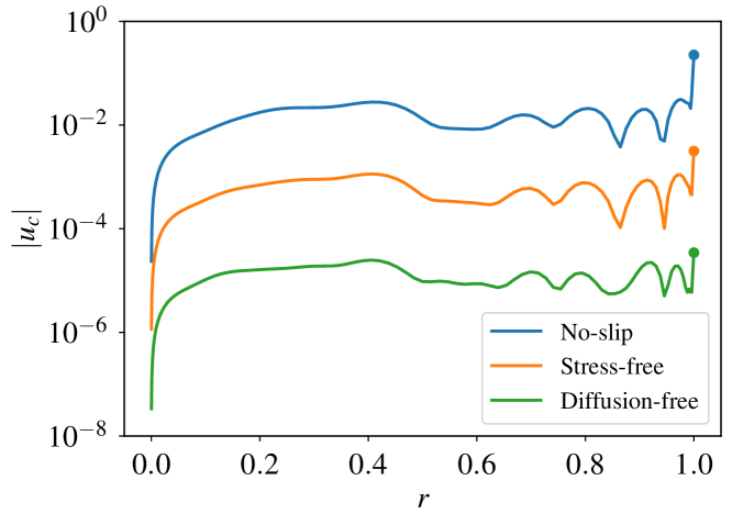
The various corrective viscous velocities $\mathbf{u}_{c}(r,z)$ are shown in Figures 2-4 for $E=10^{-4}$, $10^{-5}$ and $10^{-6}$ for the different choices of boundary conditions. Due to the vastly different amplitudes of these flows, the leading viscous scaling with $E$ is removed before contouring. That is, for non-slip boundary conditions, we expect $\mathbf{u}_{c}$ to be $O(1)$ in the boundary layer so there is no rescaling in this case whereas for the stress-free case, $\mathbf{u}_{c}$ is $O(E^{1/2})$, so $\log_{10}|\mathbf{u}_{c}/E^{1/2}|$ is plotted and $\log_{10}|\mathbf{u}_{c}/E|$ for the diffusion-free case. The various maximum amplitudes are collected in Table 3 confirming the expected scaling. The formation of internal shear layers is already evident at $E=10^{-4}$ for the non-slip and diffusion-free conditions and these get more intense and narrower as $E$ decreases (their thickness is $E^{1/3}$). Unfortunately for our purposes here, they are completely absent from the stress-free situation for reasons already mentioned.

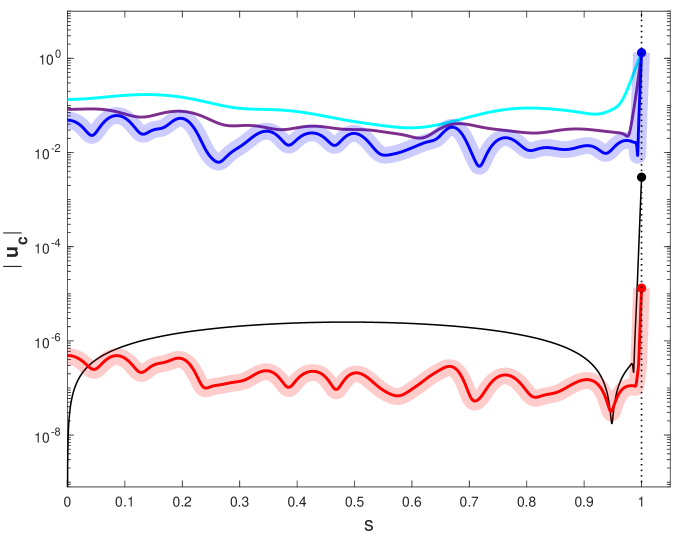
Finally, figure 5 shows the unscaled amplitude of $\mathbf{u}_{c}$ as a function of $s$ at a given $z$. The top three curves are for the non-slip situation for $E=10^{-4}$, $10^{-5}$ and $10^{-6}$ and show how the internal shear layers only really become prominent at $E=10^{-6}$. All have the same $O(1)$ value at the side wall ($=-|\mathbf{u}_{111}(1,z)|$). The thin black line is the stress-free profile at $E=10^{-6}$ which has an $O(E^{1/2})$ boundary value and is largely featureless in the interior as already commented on. Finally the lowest thick red line (computed with $N=90$) and the thin red line through its centre (computed with $N=110$) are for the diffusion-free conditions. This is an $O(E^{1/2})$ smaller than the non-slip flow everywhere. Perhaps, not surprisingly, the velocity profiles are largely similar in shape as they are formed by the same geometrical effects (the reflections of the internal shear layers) but the point is, of course, their magnitude is very different.

Table 3: Maximum amplitude of the viscous correction velocity $|\mathbf{u}_{c}(r,z)|$ over the cylindrical domain.

$E$		non-slip		stress-free		diffusion-free
$10^{-4}$		$4.24$		$3.03\sqrt{E}$		$44.56E$
$10^{-5}$		$4.24$		$3.00\sqrt{E}$		$43.48E$
$10^{-6}$		$4.24$		$2.99\sqrt{E}$		$42.35E$

Figure 5: The magnitude of the unscaled corrective viscous velocity, $|\mathbf{u}_{c}|(s,z^{*})$, plotted as a function of $s$ for a fixed choice of $z^{*}$ and various different boundary conditions. The upper 3 (blue, purple and cyan) lines are for non-slip conditions with $z^{*}=d/\sqrt{2}$ (chosen to be arbitrary). The wide transparent blue line corresponds to $N=80$ and the blue line $N=90$ both at $E=10^{-6}$ confirming that the resolution is sufficient; the purple line is for $E=10^{-5}$ and the cyan line is for $E=10^{-4}$ (the corresponding dots at $s=1$ are all at $1.32$). The middle black line is for stress-free conditions at $E=10^{-6}$ ($N=100$) and uses $z^{*}=d/2$ as the interior happens to rather featureless at $z^{*}=d/\sqrt{2}\approx 1.4$ - e.g. see figure 4(middle) (the black dot is at $2.99\times 10^{-3}$). The lower red curves are for diffusion-free conditions with $z^{*}=d/\sqrt{2}$ again. The wide transparent red line uses $N=90$ and the thin red line threading it has $N=110$ (the red dot is at $1.32\times 10^{-5}$). This plot emphasizes the difference in scales of the boundary-induced flows between the different boundary conditions and how the interior structure starts to emerge at $E=10^{-6}$ - note the structure for the diffusion-free conditions is very similar to that for the non-slip conditions albeit 4 orders or magnitude smaller.

5 Inertial wave problem in a sphere

The inertial wave problem in a sphere (equations (10) and (11)) also has separable solutions in the inviscid limit where only the normal velocity needs to vanish at the walls. These separable solutions involve modified spheroidal coordinates ($\eta,\mu$) introduced by Bryan (1889) where

$$s=\left(\frac{4}{4-\lambda^{2}}-\eta^{2}\right)^{1/2}(1-\mu^{2})^{1/2},\quad z=\left(\frac{4}{\lambda^{2}}-1\right)^{1/2}\eta\mu.$$ (24)

Using these, the pressure field can be written as (e.g. see Greenspan (1968); Zhang & Liao (2017))

$$\Phi_{mnk}=P_{n}^{m}(\eta/c_{mnk})P_{n}^{m}(\mu)\mathrm{e}^{\mathrm{i}(m\phi+\lambda t)}$$ (25)

where $P_{n}^{m}$ represents an associated Legendre function and $c_{mnk}=(1-\lambda_{mnk}^{2}/4)^{-1/2}$. The real frequency $\lambda_{mnk}$ is the $k$th eigenvalue solution of the transcendental equation

$$mP_{n}^{m}(\lambda/2)=2\left(1-\frac{\lambda^{2}}{4}\right)\frac{d}{d\lambda}P^{m}_{n}(\lambda/2),$$ (26)

and so each inertial mode is uniquely specified by a triplet of indices $(m,n,k)$.

5.1 Numerical Implementation

The viscous problem ($E\neq 0$) is numerically solved using a pseudo-spectral method based on an expansion of spherical harmonics on spherical surfaces and Chebyshev collocation in the radial direction. The incompressible condition $\nabla\cdot\mathbf{u}=0$ is fulfilled by the the toroidal-poloidal decomposition

$$\mathbf{u}=\mbox{\boldmath$\nabla$}\times(\mathcal{T}\mathbf{\hat{r}})+\mbox{\boldmath$\nabla$}\times\mbox{\boldmath$\nabla$}\times(\mathcal{P}\mathbf{\hat{r}})$$ (27)

and, for an inertial wave with the azimuthal wavenumber $m$, the scalars $\mathcal{T}$ and $\mathcal{P}$ are expanded in spherical harmonics

$$\mathcal{T}=\sum_{n=m}^{N}\mathcal{T}_{n}(r)Y_{n}^{m}(\theta,\phi),\qquad\mathcal{P}=\sum_{n=m}^{N}\mathcal{P}_{n}(r)Y_{n}^{m}(\theta,\phi).$$ (28)

where $(r,\theta,\phi)$ are spherical polar coordinates. The projections $\mathbf{\hat{r}}\cdot\mbox{\boldmath$\nabla$}\times$ and $\mathbf{\hat{r}}\cdot\mbox{\boldmath$\nabla$}\times\mbox{\boldmath$\nabla$}\times$ of the equation

$$\mathrm{i}\lambda\mathbf{u}+2\mathbf{\hat{z}}\times\mathbf{u}+\mbox{\boldmath$\nabla$}p=E\nabla^{2}\mathbf{u}$$ (29)

onto spherical harmonics, give a set of ODEs for $\mathcal{T}_{n}(r)$ and $\mathcal{P}_{n}(r)$ with a block tri-diagonal matrix structure. For the radial dependence, Chebyshev collocation is used on the $K+1$ Gauss-Lobatto nodes with the projected ODEs replaced by corresponding boundary conditions on the boundary nodes.

5.2 Boundary Conditions

The non-slip boundary conditions $\mathbf{u}={\bf 0}$ correspond to

$$\mathcal{T}_{n}(r)=0,\quad\mathcal{P}_{n}(r)=0\quad\&\quad\frac{d\mathcal{P}_{n}(r)}{dr}=0$$ (30)

at the boundary $r=1$ (the sphere radius $R$ is used to define the Ekman number as $E:=\nu/\Omega R^{2}$).

The stress-free boundary conditions are

$$u_{r}=0,\quad\frac{\partial}{\partial r}\left(\frac{u_{\theta}}{r}\right)=0,\quad\frac{\partial}{\partial r}\left(\frac{u_{\phi}}{r}\right)=0,$$ (31)

which translates into

$$\mathcal{P}_{n}(r)=0,\quad 2\frac{d\mathcal{P}_{n}(r)}{dr}-r\frac{d^{2}\mathcal{P}_{n}(r)}{dr^{2}}=0,\quad 2\mathcal{T}_{n}(r)-r\frac{d\mathcal{T}_{n}(r)}{dr}=0$$ (32)

for the toroidal and poloidal components on $r=1$.

The diffusion-free boundary conditions are

$$\mathbf{u}\cdot\mathbf{\hat{r}}=0\quad\&\quad(\mbox{\boldmath$\nabla$}^{2}\mathbf{u})\times\mathbf{\hat{r}}={\bf 0}$$ (33)

at $r=1$ or

$$\mathcal{P}_{n}(r)=0,\quad r^{2}\frac{d^{3}\mathcal{P}_{n}(r)}{dr^{3}}-n(n+1)\frac{d\mathcal{P}_{n}(r)}{dr}=0,\quad r^{2}\frac{d^{2}\mathcal{T}_{n}(r)}{dr^{2}}-n(n+1)\mathcal{T}_{n}(r)=0.$$ (34)

At the origin $r=0$, we apply the regularity conditions (Reese et al., 2006)

$$\mathcal{P}_{n}=0,\quad\mathcal{T}_{n}=0,$$ (35)

for the even degree of spherical harmonics and

$$\frac{d\mathcal{P}_{n}}{dr}=0,\quad\frac{d\mathcal{T}_{n}}{dr}=0,$$ (36)

for the odd degree of spherical harmonics. The generalized eigenvalue problem is solved using an iterative method to find the least damped eigenmode around the inviscid eigenfrequency.

Figure 6: Decay rate of inertial mode (2,4,1) with the inviscid eigen-frequency $\lambda_{241}=-1.0926$ in a sphere.

Figure 7: Viscous corrective field of the full sphere inertial mode (2,4,1) in the meridional plane for no-slip $|{\bf u}_{c}|$(left), stress-free $|{\bf u}_{c}|/\sqrt{E}$ (middle), and diffusion-free $|{\bf u}_{c}|/E$ (right) boundary conditions at $E=10^{-6}$.

Figure 8: The magnitude of the unscaled corrective viscous velocity along the dashed lines in Figure 7 for a sphere at $E=10^{-6}$.

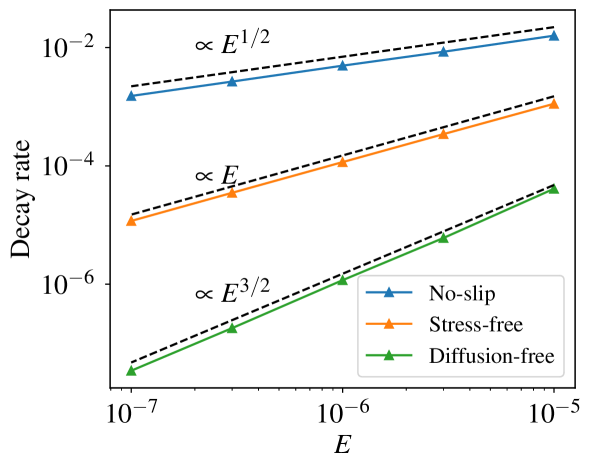
5.3 Decay rate $\lambda_{i}$ for a sphere

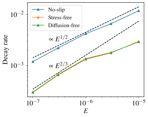
Figure 6 shows the decay rate of a typical inertial mode (here $(m,n,k)=(2,4,1)$) as a function of the Ekman number for the different boundary conditions. We find $O(E^{1/2})$ decay rates for non-slip; $O(E)$ for stress-free and $O(E^{3/2})$ for diffusion-free b.c.s. This indicates that the viscous correction in the diffusion-free situation is weakest.

Since there are $O(E)$ corrective flows driven in the interior, this last result looks anomalous until one realises that the interior dissipation contribution vanishes identically for a sphere (Zhang et al., 2001) and a spheroid (Zhang et al., 2004). This is easily understood after realising that the inertial waves in these geometries are polynomials in (the cylindrical radius) $s$ and $z$ (see the discussion on p118 of Kerswell (1993)) and partitioned into orthogonal vector spaces ${\mathscr{V}}_{n}$ where $n$ is the order of the polynomial (see p125 in Kerswell (1993)). The interior dissipation integral is then

$$\int\mathbf{u}_{0}^{*}\cdot\nabla^{2}\mathbf{u}_{0}\,dV=\frac{4}{\lambda^{2}}\int\mathbf{u}_{0}^{*}\cdot\frac{\partial^{2}\mathbf{u}_{0}}{\partial z^{2}}\,dV=0$$ (37)

as $\partial^{2}\mathbf{u}_{0}/\partial z^{2}\in{\mathscr{V}}_{n-2}$ and hence orthogonal to $\mathbf{u}_{0}\in{\mathscr{V}}_{n}$. This explains why the dissipation doesn’t vanish for a cylinder (inertial waves are not polynomials) but does also for an ellipsoidal (inertial waves are polynomials in $x$, $y$ and $z$) - see §5 of Vantieghem (2014).

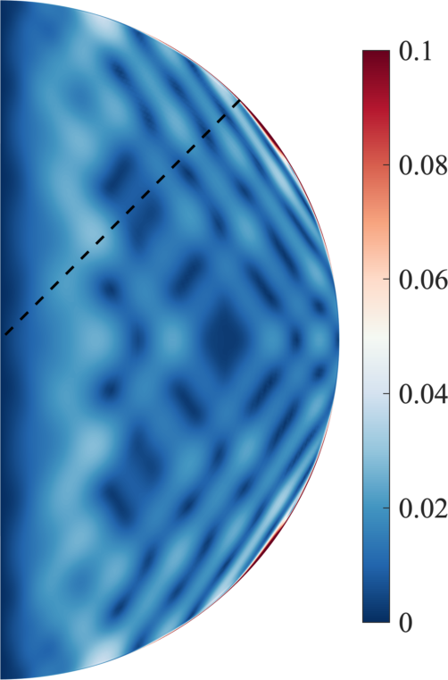
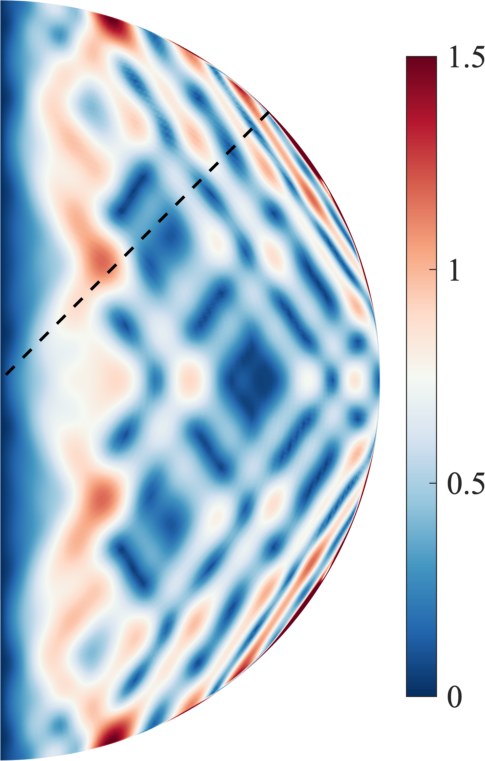
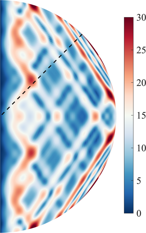
Figures 7 and 8 show the corrective viscous velocity defined in equation (22) for the inertial mode (2,4,1). This is consistent with figure 6 in showing that the diffusion-free boundary conditions lead to a smaller viscous corrective flow than stress-free boundary conditions. In particular, the stress-free boundary conditions give a corrective viscous velocity $O(E^{1/2})$ smaller than the nonslip case everywhere due to the interior viscous shear layers, while the diffusion-free solution is fully $O(E)$ smaller.

6 Inertial wave problem for a spherical shell

A spherical shell is an interesting singular geometry for the inertial wave problem as smooth inertial modes do not exist in the inviscid limit except for purely toroidal modes where the radial flow is zero everywhere. By adding a small viscosity, inertial waves exist in the form of conical shear layers spawned from the critical latitudes, though large scale structure may be hidden beneath localized shear layers at certain frequencies (Lin & Ogilvie, 2021). Figure 9 shows the decay rate of an inertial wave with $m=2$ in a spherical shell of inner-to-outer radius ratio of 0.5. Now there is no obvious reduction in the corrective viscous velocity between the stress-free and diffusion-free boundary conditions. This is because there is no benefit of applying the latter if there is no solution of the inviscid problem. We would expect a benefit for the toroidal modes but have not checked this.

Figure 9: Decay rate of an inertial mode with $m=2$ and $\lambda=-1.4406$ in a spherical shell of radius ratio 0.5.

7 Discussion

In this short note, we have discussed an apparently little-known type of boundary condition that is a plausible alternative to the usual ‘stress-free’ or Neumann conditions used as the boundary conditions which do least harm to the interior when diffusive processes are very weak. Originally used in viscoelastic flow modelling, the objective here has been to show how these ‘diffusion-free” boundary conditions work for a couple of illustrative (ODE) model problems and then demonstrate that they work, as expected, for a more complicated PDE problem. The boundary layer correction is significantly weaker for the diffusion-free boundary conditions except when the diffusion-free problem doesn’t have a well-defined solution itself (the spherical shell). Even in this latter scenario, diffusion-free does no worse than Neumann.

Hopefully, these examples highlight how useful these boundary conditions could be in GAFD modelling. The boundary conditions can either be phrased as ‘turning off the diffusion at the wall’ or, equivalently for smooth solutions, imposing that the ‘diffusion term vanishes’ which in its simplest form means setting the second derivative to zero. The latter perspective is admittedly unusual: no textbooks discuss setting the second derivative to vanish at a boundary for a second order equation. Certainly for linear equations, this is because, of course, this is really just asking the linear combination of lower derivatives which define the second order derivative to vanish which is a Robin condition. The point of the first model problem is, however, to show that this can be generalised to the nonlinear setting where the exact relationship is defined by turning diffusion off.

Disclosure statement

No potential conflict of interest was reported by the authors.

Funding

YL was supported by the National Natural Science Foundation of China (Nos. 12250012, 42142034).

References

- Bryan (1889) Bryan, G.H., The Waves on a Rotating Liquid Spheroid of Finite Ellipticity. Philosophical Transactions of the Royal Society of London A: Mathematical, Physical and Engineering Sciences, 1889, 180, 187–219.
- Buffe (2017) Buffe, R. “Stabilization of the wave equation with Ventcel boundary condition” Journal de Mathematiques Pures et Appliquees, 108, 207-259, (2017)
- Denk et al. (2021) Denk, R. and Kunze, M. and Ploss, D. “The bi-Laplacian with Wentzell boundary conditions on Lipschitz domains” Integral Equations and Operator Theory, 93, 13 (26 pages), (2021)
- Feller (1952) Feller, W. “The parabolic differential equations and the asscoiated semi-groups of transformations” Ann. of Math. 55, 468-519, (1952)
- Greenspan (1968) Greenspan, H. P. “The Theory of Rotating Fluids” Cambridge University Press, 1968.
- He et al. (2022) He, J. and Favier, B. and Rieutrod, M. and Le Dizes, S. “Internal shear layers in librating spherical shells: the case of periodic characteristic paths” J. Fluid Mech. 939 A3 (30 pages), 2022.
- He et al. (2023) He, J. and Favier, B. and Rieutord, M. and Le Dizes, S. “Internal shear layers in librating spherical shells: the case of attractors” J. Fluid Mech. submitted, 2023.
- Hinz et al. (2018) Hinz, M. and Lancia, M. R. and Teplyaev, A. and Vernole, P. “Fractal snowflake domain diffusion with boundary and interior drifts” J. Mathematical Analysis and Applications, 2018, 672-693, 2018.
- Le Dizes (2023) Le Dizes, S. “Critical slope singularities in rotating and stratified fluids”, preprint 2023.
- Kelvin (1880) Kelvin, Lord. “Vibrations of a columnar vortex” Phil. Mag., 10, 155-168, 1880.
- Kerswell (1993) Kerswell, R. R. “The Instability of precessing flow’ Geophys. Astrophys. Fluid Dynam. 72 107-144, 1993.
- Kerswell & Barenghi (1995) Kerswell, R. R. and Barenghi, C. F. “Decay of inertial waves in a rotating circular cylinder’ J. Fluid Mech. 285 203-214, 1995.
- Kerswell (1999) Kerswell, R. R. “Secondary instabilities in rapidly rotating fluids: inertial wave breakdown’ J. Fluid Mech. 382 283-306, 1999.
- Lin & Ogilvie (2021) Lin, Y. and Ogilvie, G. I. “Resonant tidal responses in rotating fluid bodies: global modes hidden beneath localised wave beams’ Ap. J. Lett. 918 L21 (7 pages), 2021.
- McEwan (1970) McEwan, A. D. Inertial oscillations in a rotating fluid cylinder” J. Fluid Mech. 40, 603-640, 1970.
- Poincare (1910) Poincaré, H. “Sur la précession des corps déformables” Bull. Astronomique, 27, 321-356, 1910.
- Reese et al. (2006) Reese, D., Lignières, F. and Rieutord, M., Acoustic oscillations of rapidly rotating polytropic stars. Astronomy & Astrophysics, 2006, 455, 621–637.
- Sureshkumar & Beris (1995) Sureshkumar, R and Beris, Antony N “Effect of artificial stress diffusivity on the stability of numerical calculations ans the dynamics of time-dependent viscoelastic flows” J. Non-Newtonian Fluid Mech., 60, 53-80, 1995.
- Sureshkumar et al. (1997) Sureshkumar, R. and Beris, A. N. and Handler, R. A., “Direct numerical simulation of the turbulent channel flow of a polymer solution” Phys. of Fluids, 9, 743-755, 1997.
- Vantieghem (2014) Vantieghem, S. “Inertial modes in a rotating triaxial ellipsoid’ Proc. Roy. Soc. A 470 20140093, 2014.
- Ventcel (1959) Ventcel, A. D. “On boundary conditions for multidimensional diffusion processes” Theor. Probab. Appl. IV, no 2, 164-177, (1959)
- Vidal & Cebron (2023) Vidal, J. and Cebron, D. “Precession-driven flows in stress-free ellipsoids’ J. Fluid Mech. 954 A5, 2023.
- Zhang & Liao (2017) Zhang, K. and Liao, X. “Theory and Modelling of Rotating Fluids” Cambridge University Press, 2017.
- Zhang et al. (2001) Zhang, K. and Earnshaw, P. and Liao, X. and Busse, F. H. “On inertial waves in a rotating fluid sphere” J. Fluid Mech. 437, 103-119, 2001.
- Zhang et al. (2004) Zhang, K. and Liao, X. and Earnshaw, P. “On inertial waves and oscillations in a rapidly rotating fluid spheroid” J. Fluid Mech. 504, 1-40, 2004.