The weighted and shifted seven-step BDF method
for parabolic equations

Georgios Akrivis Department of Computer Science and Engineering, University of Ioannina, 451 10 Ioannina, Greece, and Institute of Applied and Computational Mathematics, FORTH, 700 13 Heraklion, Crete, Greece akrivis@ cse.uoi.gr Minghua Chen School of Mathematics and Statistics, Gansu Key Laboratory of Applied Mathematics and Complex Systems, Lanzhou University, Lanzhou 730000, P.R. China chenmh@ lzu.edu.cn  and  Fan Yu School of Mathematics and Statistics, Gansu Key Laboratory of Applied Mathematics and Complex Systems, Lanzhou University, Lanzhou 730000, P.R. China yuf20@ lzu.edu.cn
Abstract.

Stability of the BDF methods of order up to five for parabolic equations can be established by the energy technique via Nevanlinna–Odeh multipliers. The nonexistence of Nevanlinna–Odeh multipliers makes the six-step BDF method special; however, the energy technique was recently extended by the authors in [Akrivis et al., SIAM J. Numer. Anal.  59 (2021) 2449–2472] and covers all six stable BDF methods. The seven-step BDF method is unstable for parabolic equations, since it is not even zero-stable. In this work, we construct and analyze a stable linear combination of two non zero-stable schemes, the seven-step BDF method and its shifted counterpart, referred to as WSBDF7 method. The stability regions of the WSBDF$q,q\leqslant 7$, with a weight $\vartheta\geqslant 1$, increase as $\vartheta$ increases, are larger than the stability regions of the classical BDF$q,$ corresponding to $\vartheta=1$. We determine novel and suitable multipliers for the WSBDF7 method and establish stability for parabolic equations by the energy technique. The proposed approach is applicable for mean curvature flow, gradient flows, fractional equations and nonlinear equations.

Key words and phrases:
Weighted and shifted seven-step BDF method, multipliers, parabolic equations, stability estimate, energy technique
2010 Mathematics Subject Classification:
Primary 65M12, 65M60; Secondary 65L06.

1. Introduction

Let $T>0,u^{0}\in H,$ and consider the initial value problem of seeking $u\in C((0,T];{\mathscr{D}}(A))\cap C([0,T];H)$ satisfying

(1.1) $$\left\{\begin{aligned} &u^{\prime}(t)+Au(t)=f(t),\quad 0<t<T,\\ &u(0)=u^{0},\end{aligned}\right.$$

with $A$ a positive definite, selfadjoint, linear operator on a Hilbert space $(H,(\cdot,\cdot))$ with domain ${\mathscr{D}}(A)$ dense in $H$ and $f:[0,T]\to H$ a given forcing term. We shall analyze the discretization of (1.1) by the weighted and shifted $q$-step backward difference formula (WSBDF$q$) with $q=7$, described by a weight $\vartheta>0$ and the corresponding characteristic polynomials $\alpha$ and $\beta,$

(1.2) $$\alpha(\zeta):=\vartheta a(\zeta)+(1-\vartheta)\tilde{a}(\zeta)=\sum_{j=0}^{q}\alpha_{j}\zeta^{j},\quad\beta(\zeta):=\vartheta\zeta^{q}+(1-\vartheta)\zeta^{q-1},~{}q\leqslant 7,$$

with $a$ and $\tilde{a}$ the characteristic polynomials of the $q$-step BDF method and the shifted $q$-step BDF method, respectively, for $1\leqslant q\leqslant 7$,

(1.3) $$\left\{\begin{aligned} &a(\zeta)=\sum_{j=1}^{q}\frac{1}{j}\zeta^{q-j}(\zeta-1)^{j}=\sum_{j=0}^{q}a_{j}\zeta^{j},\\ &\tilde{a}(\zeta)=a(\zeta)-\sum_{j=2}^{q}\frac{1}{j-1}\zeta^{q-j}(\zeta-1)^{j}=\sum_{j=0}^{q}\tilde{a}_{j}\zeta^{j}.\end{aligned}\right.$$

In particular, $\tilde{a}(\zeta)=a(\zeta)$ for $q=1$.

Let $N\in{\mathbb{N}},\tau:=T/N$ be the time step, and $t_{n}:=n\tau,n=0,\dotsc,N,$ be a uniform partition of the interval $[0,T].$ We recursively define a sequence of approximations $u^{m}$ to the nodal values $u(t_{m})$ of the exact solution by the WSBDF7 method,

(1.4) $$\sum_{i=0}^{7}\alpha_{i}u^{n+i}+\vartheta\tau Au^{n+7}+(1-\vartheta)\tau Au^{n+6}=\vartheta\tau f^{n+7}+(1-\vartheta)\tau f^{n+6}$$

for $n=0,\dotsc,N-7,$ with $f^{m}:=f(t_{m}),$ assuming that starting approximations $u^{0},\dotsc,u^{6}$ are given. For convenience, we suppressed the dependence of $\alpha$ and of its coefficients on $\vartheta.$ We are particularly interested in the WSBDF7 method (1.4) for $\vartheta=3,$

(1.5) $$\sum_{i=0}^{7}\alpha_{i}u^{n+i}+3\tau Au^{n+7}-2\tau Au^{n+6}=3\tau f^{n+7}-2\tau f^{n+6},\quad n=0,\dotsc,N-7.$$

Let $P_{7}\in{\mathbb{P}}_{7}$ be the Lagrange interpolating polynomial of a function $y$ at the nodes $t_{n},t_{n+1},\dotsc,t_{n+7}.$ We recall that the seven-step BDF method,

(1.6) $$\sum_{i=0}^{7}a_{i}y^{n+i}=\tau f(t_{n+7},y^{n+7}),$$

for an o.d.e. $y^{\prime}=f(t,y)$, is constructed by approximating the derivative of $y$ at the node $t_{n+7}$ in the relation $y^{\prime}(t_{n+7})=f\big{(}t_{n+7},y(t_{n+7})\big{)}$ by the derivative $P_{7}^{\prime}(t_{n+7})$ of the interpolating polynomial. Analogously, the shifted seven-step BDF method,

(1.7) $$\sum_{i=0}^{7}\tilde{a}_{i}y^{n+i}=\tau f(t_{n+6},y^{n+6}),$$

is constructed by approximating $y^{\prime}(t_{n+6})$ in the relation $y^{\prime}(t_{n+6})=f\big{(}t_{n+6},y(t_{n+6})\big{)}$ by $P_{7}^{\prime}(t_{n+6}).$ Notice that $\vartheta P_{7}^{\prime}(t_{n+7})+(1-\vartheta)P_{7}^{\prime}(t_{n+6})$ is, in general, different from $P_{7}^{\prime}(t_{n+6}+\vartheta\tau)$.

Multiplying (1.6) and (1.7) by $\vartheta$ and $1-\vartheta,$ respectively, and adding the results, we obtain the weighted and shifted BDF7 (WSBDF7) method,

(1.8) $$\vartheta\sum_{i=0}^{7}a_{i}y^{n+i}+(1-\vartheta)\sum_{i=0}^{7}\tilde{a}_{i}y^{n+i}=\vartheta\tau f(t_{n+7},y^{n+7})+(1-\vartheta)\tau f(t_{n+6},y^{n+6}).$$

In particular, for $\vartheta=1$ and $\vartheta=0,$ the WSBDF7 method reduces to the standard seven-step BDF method and to the corresponding SBDF method.

It is well known that both methods, BDF7 and SBDF7, are not zero-stable; for BDF7, see, e.g., [11, Theorem 3.4]; concerning SBDF7, it is easily seen that $\tilde{a}(-13)\tilde{a}(-12)<0,$ whence $\tilde{a}$ has a root in the interval $(-13,-12).$ The order of both methods is $7.$ Here, we show that their combination, WSBDF7, is $A(\varphi)$-stable for $\vartheta=3$, stable even for parabolic equations.

The explicit form of the polynomials $a$ and $\tilde{a}$ in (1.3) with $q=7$ is

$$\begin{split}a(\zeta)&=\frac{1}{420}\big{(}1089\zeta^{7}-2940\zeta^{6}+4410\zeta^{5}-4900\zeta^{4}+3675\zeta^{3}-1764\zeta^{2}+490\zeta-60\big{)},\\ \tilde{a}(\zeta)&=\frac{1}{420}\big{(}60\zeta^{7}+609\zeta^{6}-1260\zeta^{5}+1050\zeta^{4}-700\zeta^{3}+315\zeta^{2}-84\zeta+10\big{)}.\end{split}$$

Let $|\cdot|$ denote the norm on $H$ induced by the inner product $(\cdot,\cdot)$, and introduce on $V,V:={\mathscr{D}}(A^{1/2}),$ the norm $\|\cdot\|$ by $\|v\|:=|A^{1/2}v|.$ We identify $H$ with its dual, and denote by $V^{\prime}$ the dual of $V$, and by $\|\cdot\|_{\star}$ the dual norm on $V^{\prime},\|v\|_{\star}=|A^{-1/2}v|.$ We shall use the notation $(\cdot,\cdot)$ also for the antiduality pairing between $V^{\prime}$ and $V.$ For simplicity, we denote by $\langle\cdot,\cdot\rangle$ the inner product on $V,$ $\langle v,w\rangle:=(A^{1/2}v,A^{1/2}w).$

Our stability results are established by the energy technique utilizing suitable multipliers, and are given in the following two theorems and in a corollary.

Theorem 1.1 (Stability of method (1.5)).

Let $u^{0},u^{1},\dotsc,u^{6}\in V.$ The WSBDF7 method (1.5) is stable in the sense that

(1.9) $$|u^{n}|^{2}+\tau\|u^{n}\|^{2}\leqslant C\sum_{j=0}^{6}\big{(}|u^{j}|^{2}+\tau\|u^{j}\|^{2}\big{)}+C\tau\sum_{\ell=6}^{n}\|f^{\ell}\|_{\star}^{2},\quad n=7,\dotsc,N.$$

Here $C$ denotes a generic constant, independent of $T$ and the operator $A$ as well as of $f,\tau,$ and $n$.

Theorem 1.2 (Second stability estimate).

Let $u^{0},u^{1},\dotsc,u^{6}\in V,$ and let us indicate by a dot the application of the $7$-step weighted and shifted backward difference operator,

(1.10) $$\dot{v}^{m}:=\frac{1}{\tau}\sum_{i=0}^{7}\alpha_{i}v^{m-7+i},\quad m=7,\dotsc,N.$$

The WSBDF7 method (1.5) is stable in the sense that

(1.11) $$\|u^{n}\|^{2}+\tau|\dot{u}^{n}|^{2}\leqslant C\sum_{j=0}^{6}\|u^{j}\|^{2}+C\tau\sum_{\ell=6}^{n}|f^{\ell}|^{2},\quad n=7,\dotsc,N.$$

Here $C$ denotes a generic constant as in Theorem 1.1.

Corollary 1.1 (Third stability estimate).

Let $u^{0},u^{1},\dotsc,u^{6}\in V,$ and let us denote by $\partial_{\tau}u^{n}:=(u^{n}-u^{n-1})/\tau,n=1,\dotsc,N,$ the backward difference quotients. The WSBDF7 method (1.5) is stable in the sense that

(1.12) $$\|u^{n}\|^{2}+\tau|\partial_{\tau}u^{n}|^{2}\leqslant C\sum_{j=0}^{6}\|u^{j}\|^{2}+C\tau\sum_{j=1}^{6}|\partial_{\tau}u^{j}|^{2}+C\tau\sum_{\ell=6}^{n}|f^{\ell}|^{2},\quad n=7,\dotsc,N,$$

with a generic constant $C.$

The application of the energy technique to establish stability of high order multistep methods for parabolic equations relies on suitable multipliers. The multiplier technique was introduced by Nevanlinna and Odeh in [17] and is based on Dahquist’s equivalence between A- and G-stability; see also [12, §V.8, pp. 342–347]. In [17], suitable multipliers for the three-, four- and five-step BDF methods were determined; see also [3] for optimal Nevanlinna–Odeh multipliers for these methods, i.e., multipliers with minimal sum of absolute values.

The multiplier technique became widely known and popular after its first actual application to the stability analysis for parabolic equations by Lubich, Mansour, and Venkataraman in 2013; see [16]. In recent years, the energy technique has been frequently used in the analyses of various variants of BDF methods of order up to $5,$ such as fully implicit, linearly implicit or implicit–explicit, for a series of linear and nonlinear equations of parabolic type. Nonexistence of Nevanlinna–Odeh multipliers for the six-step BDF method was established in [1]; there, to overcome this difficulty, the notion of multipliers was slightly modified, and multipliers for the six-step BDF method were determined, which, in combination with the Grenander–Szegő theorem for symmetric banded Toeplitz matrices, made the energy technique applicable also to this method for parabolic equations with self-adjoint elliptic part.

Here, focusing on the discretization of parabolic equations with self-adjoint elliptic part by multistep methods, we first extend the notion of multipliers, and then determine suitable multipliers for the WSBDF7 method (1.5) and prove Theorems 1.1 and 1.2 by the energy technique. The new, more general notion of multipliers reduces to the corresponding notion in [1] in the case of the BDF methods; however, both the proofs and the stability results here and in [1] are different. The present approach is shorter and simpler but it yields weaker stability results, in the sense that (1.9) leads to optimal order error estimates in the discrete $\ell^{\infty}(H)$ norm but to suboptimal by half-an-order error estimates in the discrete $\ell^{\infty}(V)$ norm; see (7.2); in contrast, the stability estimates in [1] lead to optimal order error estimate in the discrete $\ell^{\infty}(H)$ as well as in the discrete $\ell^{2}(V)$ norms. Of course, (1.11) leads to optimal order error estimates in the discrete $\ell^{\infty}(V)$ norm. Let us also mention that the stability approach in [1] is restricted to BDF methods, in which case banded Toeplitz matrices enter. In the case of the WSBDF7 method (1.5), the corresponding matrices reduce to banded Toeplitz matrices only after discarding their last row and column; this fact prevents us from using the Grenander–Szegő theorem.

In 1991, linear multistep methods of orders from $2$ to $7$ for ordinary differential equations, with stability regions larger than the stability regions of the BDF method of the same order, were constructed in [15]. In particular, the seven-step methods of order $7$ of [15] are the WSBDF7 method (1.4) with a parameter $\vartheta.$ High order implicit-explicit multistep methods were constructed and analyzed in [8]. Then, in 1995, implicit-explicit multistep schemes of orders from $1$ to $4$ were constructed in [4]; the method of order $2$ in [4] coincides with the WSBDF2 method, but the methods of order $3$ and $4$ are different from the WSBDF$q,q=3,4,$ methods. The construction techniques in [15] and for the WSBDF methods are significantly different. The point of departure in [15] is the polynomial $\beta$ in (1.2); the corresponding polynomial $\alpha$ is then determined via the order conditions. Here, the WSBDF7 method (1.8) is constructed by the simpler, direct, and more efficient weighted and shifted technique, which immediately extends also to variable time step schemes. For example, the variable time-step WSBDF3 methods for parabolic equations are presented in [6]. However, there is no published work for variable or even uniform time-step WSBDF$q,q\geqslant 4,$ methods.

The proposed methods, for $q\leqslant 6,$ including the classical case $\vartheta=1$, have been recently widely used to various applied scientific phenomena, such as mean curvature flow [10, 14], gradient flows [13], and fractional equations [7].

An outline of the paper is as follows: In the short Section 2, we briefly comment on the stability regions of the WSBDF7 method (1.8) for various values of the parameter $\vartheta.$ In Section 3, we make precise the requirements on the multipliers for multistep methods that are suitable for our stability approach, and show that our notion extends the multiplier notion of [1] for BDF methods. The remaining part of the article is devoted to the WSBDF7 method (1.5). First, in Section 4 we give a suitable multiplier for this method and in Section 5 comment on the determination of such multipliers; in particular, we provide information about the range of such multipliers with up to the first four nonvanishing components. Sections 6 and 7 are devoted to the proof of the stability estimates (1.9) and (1.11), and to the derivation of error estimates. We conclude in Section 8 with numerical results.

2. Stability regions

The BDF$q$ methods are $A(\varphi_{q})$-stable with $\varphi_{1}=\varphi_{2}=90^{\circ}$, $\varphi_{3}\approx 86.03^{\circ},\varphi_{4}\approx 73.35^{\circ},\varphi_{5}\approx 51.84^{\circ},$ and $\varphi_{6}\approx 17.84^{\circ}$; see [12, Section V.2]. The WSBDF$q$ methods are $A(\tilde{\varphi}_{q})$-stable with $\tilde{\varphi}_{1}=\tilde{\varphi}_{2}=90^{\circ}$, $\tilde{\varphi}_{3}\approx 89.55^{\circ},\tilde{\varphi}_{4}\approx 85.32^{\circ},\tilde{\varphi}_{5}\approx 73.2^{\circ},$ and $\tilde{\varphi}_{6}\approx 51.23^{\circ},$ for the weights $\vartheta_{3}=20,\vartheta_{4}=60,\vartheta_{5}=48,\vartheta_{6}=50,$ respectively; see [15, Table 2]. Notice that $\varphi_{q}<\tilde{\varphi}_{q}<\varphi_{q-1}$ for $q=3,4,5,6.$ It can also be shown that $\tilde{\varphi}_{q}\to\varphi_{q-1}$ as $\vartheta\to\infty$ for $q=3,\dotsc,7;$ see Remark 2.1. It seems that the value $\tilde{\varphi}_{7}\approx 18.32^{\circ}>\varphi_{6}\approx 17.84^{\circ}$ for $\vartheta_{7}=200/7$ given in [15] is incorrect. We numerically computed the approximations $\tilde{\varphi}_{1}=\tilde{\varphi}_{2}=90^{\circ},\tilde{\varphi}_{3}\approx 89.99^{\circ},\tilde{\varphi}_{4}\approx 85.93^{\circ},\tilde{\varphi}_{5}\approx 73.2^{\circ}$, $\tilde{\varphi}_{6}\approx 51.63^{\circ},$ and $\tilde{\varphi}_{7}\approx 17.47^{\circ}$ for the weight $\vartheta=100$.

Remark 2.1 (The limit of the stability angles $\tilde{\varphi}_{q}$ of WSBDF$q$).

Nørsett, [18, p. 263], established an A$(\varphi_{q})$-stability criterion for the BDF$q$ methods, namely, in his notation,

$$\tan(\varphi_{q})=\min_{x\in D_{q}}\left(-\sqrt{1-x^{2}}\cdot\frac{I_{q}(x)}{R_{q}(x)}\right),\quad D_{q}=\{x\in[-1,1],R_{q}(x)<0\};$$

here $I_{q}(x)$ and $R_{q}(x)$ are related to the imaginary and real parts of points on the root locus curve of the method, and are expressed in terms of the Chebyshev polynomials. Using this criterion and results in [15, p. 7], we have

$$\tan(\tilde{\varphi}_{q})=\min_{x\in\tilde{D}_{q}}\left(-\sqrt{1-x^{2}}\cdot\lim_{\vartheta\rightarrow\infty}\frac{\tilde{I}_{q}(x)}{\tilde{R}_{q}(x)}\right),\quad\tilde{D}_{q}=\{x\in[-1,1],\tilde{R}_{q}(x)<0\}$$

for the stability angle $\tilde{\varphi}_{q}$ of the WSBDF$q$ method. Now, we can easily check that

$$\lim_{\vartheta\rightarrow\infty}\frac{\tilde{I}_{q}(x)}{\tilde{R}_{q}(x)}=\frac{I_{q-1}(x)}{R_{q-1}(x)},\quad q=3,\dotsc,7,$$

and infer that

$$\tilde{\varphi}_{q}\rightarrow\varphi_{q-1}\quad\text{as }\ \vartheta\to\infty,\quad q=3,\dotsc,7.$$

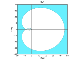
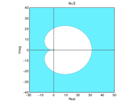
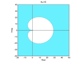
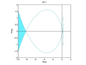
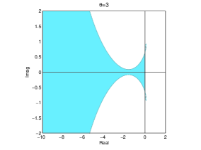
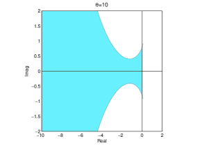
Here, we examine the stability regions of the WSBDF7 method (1.8). For the test equation $y^{\prime}(t)=\lambda y(t),\lambda\in{\mathbb{C}}$, the method reads

(2.1) $$\sum_{i=0}^{7}\alpha_{i}y^{n+i}=\lambda\tau\vartheta y^{n+7}+\lambda\tau(1-\vartheta)y^{n+6},\quad n=0,\dotsc,N-7.$$

To study the stability regions, we set $z=\lambda\tau$ in (2.1) and consider the characteristic polynomial

$$p(\zeta):=\alpha(\zeta)-z\beta(\zeta),\quad\zeta\in{\mathbb{C}};$$

again, for convenience, we suppressed the dependence of the polynomials $\alpha$ and $\beta$ on $\vartheta;$ see (1.2). Then, the stability region of the method is the set of all $z\in\mathbb{C}$ such that the characteristic polynomial $p$ satisfies the root condition. We plot the stability regions of the WSBDF7 method (2.1) for $\vartheta=1,3,10$ in Figure 2.1. Notice that the stability regions increase as $\vartheta$ increases.

Refer to caption   Refer to caption   Refer to caption
Figure 2.1. The stability regions $($upper panel$)$ as well as zoom in around the origin $($lower panel$)$, in light blue, for $\vartheta=1,3,10$, respectively.

3. Multipliers for multistep methods

Here, we extend the notion of multipliers for multistep methods applied to parabolic equations with self-adjoint elliptic part. The present, more general notion of multipliers reduces to the corresponding notion in [1] in the case of the BDF methods. The multiplier technique hinges on the celebrated equivalence of A- and G-stability for multistep methods by Dahlquist.

Lemma 3.1 ([9]; see also [5] and [12, Section V.6]).

Let $\rho(\zeta)=\rho_{q}\zeta^{q}+\dotsb+\rho_{0}$ and $\sigma(\zeta)=\sigma_{q}\zeta^{q}+\dotsb+\sigma_{0}$ be polynomials of degree $q,$ with real coefficients, that have no common divisor. Let $(\cdot,\cdot)$ be a real inner product with associated norm $|\cdot|.$ If

(A) $$\operatorname{Re}\frac{\rho(\zeta)}{\sigma(\zeta)}>0\quad\text{for }\,|\zeta|>1,$$

then there exists a positive definite symmetric matrix $G=(g_{ij})\in{\mathbb{R}}^{q,q}$ and real $\gamma_{0},\dotsc,\gamma_{q}$ such that for $v^{0},\dotsc,v^{q}$ in the inner product space,

(G) $$\Big{(}\sum_{i=0}^{q}\rho_{i}v^{i},\sum_{j=0}^{q}\sigma_{j}v^{j}\Big{)}=\sum_{i,j=1}^{q}g_{ij}(v^{i},v^{j})-\sum_{i,j=1}^{q}g_{ij}(v^{i-1},v^{j-1})+\Big{|}\sum_{i=0}^{q}\gamma_{i}v^{i}\Big{|}^{2}.$$

Let us briefly comment on the assumption that $\rho$ and $\sigma$ are polynomials of the same degree; obviously, if (A) would be satisfied for polynomials of different degrees, then explicit A-stable methods would exist. First, nonconstant polynomials cannot satisfy (A) since they cannot pertain the sign of their real part as $|z|\to\infty.$ This shows also that the degree of $\rho$ cannot exceed the degree of $\sigma,$ since then we could write $\rho/\sigma$ as the sum of a nonconstant polynomial and a rational function $R$ such that the degree of its numerator is lower than the degree of its denominator, whence, in particular, $\lim_{|z|\to\infty}\operatorname{Re}R(z)=0.$ Finally, (A) is symmetric with respect to $\rho$ and $\sigma$ since $\operatorname{Re}[\rho(z)/\sigma(z)]\operatorname{Re}[\sigma(z)/\rho(z)]=\cos^{2}\varphi>0$ for $\rho(z)/\sigma(z)=r{\rm e}^{{\rm i}\varphi}$ not purely imaginary.

Next, we specify our requirements on the multipliers; in Section 4, we shall provide motivation for these requirements.

Definition 3.1 (Multipliers).

Let $\alpha$ and $\beta$ be the characteristic polynomials of an A$(0)$-stable $q$-step method; then, $\alpha_{q}\beta_{q}>0,$ and thus we can assume that the leading coefficients $\alpha_{q}$ and $\beta_{q}$ are positive. For a $q$-tuple of real numbers $(\mu_{1},\dotsc,\mu_{q})$ consider the polynomial $\mu(\zeta):=\zeta^{q}-\mu_{1}\zeta^{q-1}-\dotsb-\mu_{q}.$ Then, $(\mu_{1},\dotsc,\mu_{q})$ is called a multiplier of the method if it satisfies three properties, namely, if the pairs of polynomials $(\alpha,\mu)$ and $(\beta,\mu)$ have no common divisors, except possibly of a common factor of the form $\zeta^{\ell}$ for the pair $(\beta,\mu)$, and satisfy the A-stability condition (A) in Lemma 3.1 and a slightly more restrictive version of it, respectively, that is,

(3.1) $$\operatorname{Re}\frac{\alpha(\zeta)}{\mu(\zeta)}>0\quad\text{for }\,|\zeta|>1,$$

i.e., the method described by the coefficients of the polynomials $\alpha$ and $\mu$ is $A$-stable, and

(3.2) $$\operatorname{Re}\frac{\beta(\zeta)}{\mu(\zeta)}>c_{\star}\quad\text{for }\,|\zeta|>1,$$

for some positive constant $c_{\star},$ and the polynomial $\mu$ does not have unimodular roots.

The A-stability condition (3.1) is symmetric with respect to the polynomials $\alpha$ and $\mu,$ since for any not purely imaginary complex number $z=r{\rm e}^{{\rm i}\varphi},$ we have $\operatorname{Re}z\operatorname{Re}\frac{1}{z}=\cos^{2}\varphi>0.$ This property is crucial because otherwise the A-stability condition (A) would not be equivalent to the obviously symmetric condition (G). On the other hand, the more stringent condition (3.2) cannot be symmetric in case $\mu$ has unimodular roots, since it implies that $\beta$ does not have unimodular roots. For instance for $\mu(\zeta)=\zeta-1$ and $\beta(\zeta)=\zeta,$ i.e., for the characteristic polynomials of the implicit Euler method, we obviously have

$$\lim_{\zeta\to 1}\frac{\mu(\zeta)}{\beta(\zeta)}=0,$$

while, with $\zeta=r{\rm e}^{{\rm i}\varphi},$

$$\operatorname{Re}\frac{\beta(\zeta)}{\mu(\zeta)}=\frac{r^{2}-r\cos\varphi}{r^{2}-2r\cos\varphi+1}\quad\text{and}\quad\frac{r^{2}-r\cos\varphi}{r^{2}-2r\cos\varphi+1}\geqslant\frac{1}{2}\iff r\geqslant 1.$$

The additional condition that $\mu$ does not have unimodular roots makes condition (3.2) symmetric; cf. also Lemma 3.2.

Let us note that the third property of multipliers, i.e., that $\mu$ does not have unimodular roots, is not needed for the proof of Theorem 1.1; we will use it only in the proof of Theorem 1.2.

Remark 3.1 (Equivalent version of the conditions on the pair $(\beta,\mu)$).

Let $\ell\geqslant 0$ be the largest integer such that $\zeta^{\ell}$ is a common factor of $\beta$ and $\mu.$ We factor $\zeta^{\ell}$ out, and write $\beta$ and $\mu$ in the form

(3.3) $$\beta(\zeta)=\zeta^{\ell}\delta(\zeta)\quad\text{and}\quad\mu(\zeta)=\zeta^{\ell}\kappa(\zeta).$$

Then, the conditions on the pair $(\beta,\mu)$ in the previous Definition can be equivalently formulated in the form: the pair of polynomials $(\delta,\kappa)$ has no common divisor and satisfies the condition

(3.4) $$\operatorname{Re}\frac{\delta(\zeta)}{\kappa(\zeta)}>c_{\star}\quad\text{for }\,|\zeta|>1,$$

for some positive constant $c_{\star}.$

The following result is an immediate consequence of the maximum principle for harmonic functions.

Lemma 3.2 (Equivalent versions of conditions (3.1) and (3.2)).

With the notation in Definition 3.1 and $\mu_{0}:=-1,$ conditions (3.1) and (3.2) are equivalent to

(3.5) $$-\sum_{j,\ell=0}^{q}\alpha_{j}\mu_{\ell}\cos((j+\ell-q)\varphi)\geqslant 0\quad\forall\varphi\in{\mathbb{R}}$$

and, if the polynomial $\mu$ does not have unimodular roots,

(3.6) $$-\sum_{j,\ell=0}^{q}\beta_{j}\mu_{\ell}\cos((j+\ell-q)\varphi)\geqslant\tilde{c}_{\star}\quad\forall\varphi\in{\mathbb{R}},$$

for some positive constant $\tilde{c}_{\star},$ respectively.

Proof.

The rational functions $\alpha/\mu$ and $\beta/\mu$ are holomorphic outside the unit disk in the complex plane and

$$\lim_{|z|\to\infty}\frac{\alpha(z)}{\mu(z)}=\alpha_{q}>0,\quad\lim_{|z|\to\infty}\frac{\beta(z)}{\mu(z)}=\beta_{q}>0.$$

Therefore, according to the maximum principle for harmonic functions, (3.1) and (3.2) for $c_{\star}\leqslant\beta_{q}$ are equivalent to

$$\operatorname{Re}\big{[}\alpha(\zeta)\mu(\bar{\zeta})\big{]}\geqslant 0\quad\forall\zeta\in{\mathscr{K}},\quad\text{and}\quad\operatorname{Re}\frac{\beta(\zeta)}{\mu(\zeta)}\geqslant c_{\star}\quad\forall\zeta\in{\mathscr{K}},$$

respectively, with ${\mathscr{K}}$ the unit circle in the complex plane, ${\mathscr{K}}:=\{\zeta\in{\mathbb{C}}:|\zeta|=1\},$ i.e., equivalent to

(3.7) $$\operatorname{Re}\big{[}\alpha({\rm e}^{{\rm i}\varphi})\mu({\rm e}^{-{\rm i}\varphi})\big{]}\geqslant 0\quad\text{and}\quad\operatorname{Re}\big{[}\beta({\rm e}^{{\rm i}\varphi})\mu({\rm e}^{-{\rm i}\varphi})\big{]}\geqslant c_{\star}|\mu({\rm e}^{{\rm i}\varphi})|^{2}\quad\forall\varphi\in{\mathbb{R}}.$$

Now, $\mu(\zeta)=-\sum_{\ell=0}^{q}\mu_{\ell}\zeta^{q-\ell},$ and thus

$$\beta({\rm e}^{{\rm i}\varphi})\mu({\rm e}^{-{\rm i}\varphi})=-\sum_{j=0}^{q}\beta_{j}{\rm e}^{j{\rm i}\varphi}\sum_{\ell=0}^{q}\mu_{\ell}{\rm e}^{(\ell-q){\rm i}\varphi}=-\sum_{j,\ell=0}^{q}\beta_{j}\mu_{\ell}{\rm e}^{(j+\ell-q){\rm i}\varphi},$$

whence

$$\operatorname{Re}\big{[}\beta({\rm e}^{{\rm i}\varphi})\mu({\rm e}^{-{\rm i}\varphi})\big{]}=-\sum_{j,\ell=0}^{q}\beta_{j}\mu_{\ell}\cos((j+\ell-q)\varphi),$$

and, since $|\mu({\rm e}^{{\rm i}\varphi})|^{2}$ is bounded from above and below by positive constants, (3.6) is equivalent to the second relation in (3.7). Analogously, the first relation in (3.7) is equivalent to (3.5). ∎

Remark 3.2 (BDF methods).

In the case of the standard $q$-step BDF method, we have $\beta(\zeta)=\zeta^{q},$ whence (3.6) takes the form

$$-\sum_{\ell=0}^{q}\mu_{\ell}\cos(\ell\varphi)\geqslant\tilde{c}_{\star}\quad\forall\varphi\in{\mathbb{R}},$$

i.e., since $\mu_{0}=-1,$

(3.8) $$1-\mu_{1}\cos\varphi-\dotsb-\mu_{q}\cos(q\varphi)\geqslant\tilde{c}_{\star}\quad\forall\varphi\in{\mathbb{R}}.$$

Since $\tilde{c}_{\star}$ can be chosen arbitrarily small, (3.8) can be written as a positivity condition,

(3.9) $$1-\mu_{1}\cos\varphi-\dotsb-\mu_{q}\cos(q\varphi)>0\quad\forall\varphi\in{\mathbb{R}}.$$

Conditions (3.1), with $\alpha$ the characteristic polynomial of the $q$-step BDF method, and (3.9) were used in [1] to establish stability of BDF methods for parabolic equations with self-adjoint elliptic part by the energy technique. The motivation for the positivity condition (3.9) in [1] was that $1-\mu_{1}\cos\varphi-\dotsb-\mu_{q}\cos(q\varphi)$ was the generating function of symmetric banded Toeplitz matrices of arbitrary dimension entering into the stability analysis, and (3.9) ensured the positive definiteness of these matrices.

4. Multipliers for the WSBDF7 method (1.5)

From now on, we consider the WSBDF7 method (1.5), i.e., (1.4) with $\vartheta=3.$

As we shall see,

(4.1) $$\mu_{1}=1.6,\quad\mu_{2}=-1.6,\quad\mu_{3}=1.1,\quad\mu_{4}=-0.3,\quad\mu_{5}=\mu_{6}=\mu_{7}=0,$$

are multipliers of the method with $\tilde{c}_{\star}:=0.01$ in (3.6).

Let us now use these specific multipliers to motivate our requirements in Definition 3.1.

To prove the first stability result for method (1.5) by the energy technique, we subtract and add the term $c_{\star}A\Big{(}u^{n+7}-\sum_{j=1}^{4}\mu_{j}u^{n+7-j}\Big{)}$ from and to its left-hand side, and subsequently test by $u^{n+7}-\mu_{1}u^{n+6}-\dotsb-\mu_{7}u^{n}=u^{n+7}-\mu_{1}u^{n+6}-\dotsb-\mu_{4}u^{n+3}$ to obtain

(4.2) $$\Big{(}\sum_{i=0}^{7}\alpha_{i}u^{n+i},u^{n+7}-\sum_{j=1}^{4}\mu_{j}u^{n+7-j}\Big{)}+\tau A_{n+7}+\tau c_{\star}\Big{\|}u^{n+7}-\sum_{j=1}^{4}\mu_{j}u^{n+7-j}\Big{\|}^{2}=\tau F_{n+7},$$

$n=0,\dotsc,N-7,$ with

$$\left\{\begin{aligned} A_{n+7}&:=\Big{\langle}3u^{n+7}-2u^{n+6}-c_{\star}\Big{(}u^{n+7}-\sum_{j=1}^{4}\mu_{j}u^{n+7-j}\Big{)},u^{n+7}-\sum_{j=1}^{4}\mu_{j}u^{n+7-j}\Big{\rangle},\\ F_{n+7}&:=\Big{(}3f^{n+7}-2f^{n+6},u^{n+7}-\sum_{j=1}^{4}\mu_{j}u^{n+7-j}\Big{)}.\end{aligned}\right.$$

The term $F_{n+7}$ in (4.2) can be easily estimated from above via elementary inequalities. The term involving the approximate solutions will be absorbed in the third term on the left-hand side of (4.2); this is the motivation for the use of a positive constant $c_{\star}$ in (3.4) or in (3.2).

To estimate the first term in (4.2) from below, we shall first prove that the pair of polynomials $\alpha$ and $\mu,$ with $\alpha$ given in (1.2) for $\vartheta=3$,

(4.3) $$\begin{split}\alpha(\zeta)=\frac{1}{420}\big{(}3147\zeta^{7}&-10038\zeta^{6}+15750\zeta^{5}-16800\zeta^{4}\\ &+12425\zeta^{3}-5922\zeta^{2}+1638\zeta-200\big{)},\end{split}$$

and $\mu$ the polynomial associated to the multipliers in (4.1),

(4.4) $$\mu(\zeta)=\zeta^{7}-1.6\zeta^{6}+1.6\zeta^{5}-1.1\zeta^{4}+0.3\zeta^{3},$$

satisfy the conditions in Definition 3.1; see Proposition 4.1. This fact in combination with Lemma 3.1 will enable us to utilize a relation of the form (G).

Analogously, to estimate $A_{n+7}$ from below, in view of its specific form and, in particular, the fact that it depends only on five consecutive approximations, namely on $u^{n+3},\dotsc,u^{n+7},$ it suffices to use polynomials of degree $4.$ Thus, we factor $\zeta^{3}$ out of the polynomials $\beta$ in (1.2) for $\vartheta=3$ and $\mu$ and consider the polynomials $\delta$ and $\kappa,$

(4.5) $$\delta(\zeta):=3\zeta^{4}-2\zeta^{3},$$

and

(4.6) $$\kappa(\zeta):=\zeta^{4}-\frac{8}{5}\zeta^{3}+\frac{8}{5}\zeta^{2}-\frac{11}{10}\zeta+\frac{3}{10}=\big{(}\zeta-\frac{3}{5}\big{)}\big{(}\zeta^{3}-\zeta^{2}+\zeta-\frac{1}{2}\big{)};$$

cf. (3.3). Now, to take advantage of a relation of the form (G), given that the polynomials $\delta-c_{\star}\kappa$ and $\kappa$ enter into the first and second arguments in the inner product in $A_{n+7},$ we need to prove that the pair of polynomial $(\delta-c_{\star}\kappa,\kappa)$ satisfies the conditions in Lemma 3.1; obviously, these conditions can be reformulated in the form that the polynomials $\delta$ and $\kappa$ have no common divisor and satisfy condition (3.4). We shall prove these properties in Proposition 4.2.

Proposition 4.1 (Polynomials $\alpha$ and $\mu$ satisfy condition (3.1)).

The polynomials $\alpha$ for $\vartheta=3$ and $\mu$ of (4.3) and (4.4) do not have common divisor and satisfy condition (3.1).

Proof.

First, $\mu(\zeta)=\zeta^{3}(\zeta-3/5)\tilde{\kappa}(\zeta)$ with $\tilde{\kappa}(\zeta):=\zeta^{3}-\zeta^{2}+\zeta-1/2;$ see (4.4) and (4.6). Thus, to show that the roots of $\mu$ are inside the unit disk, it suffices to show that this is the case for $\tilde{\kappa}.$ Now,

$$\tilde{\kappa}\big{(}\frac{1}{2}\big{)}=-\frac{1}{8}<0\quad\text{and}\quad\tilde{\kappa}(1)=\frac{1}{2}>0,$$

and thus $\tilde{\kappa}$ has a real root $\zeta_{1}\in(1/2,1).$ Actually, this is the only real root of $\tilde{\kappa},$ since $\tilde{\kappa}$ is strictly increasing on the real axis,

$$\tilde{\kappa}^{\prime}(x)=3x^{2}-2x+1=2x^{2}+(x-1)^{2}>0.$$

Let $\zeta_{2},\zeta_{3}$ be the complex conjugate roots of $\tilde{\kappa}.$ Then, according to Vieta’s formulas,

$$\zeta_{1}\zeta_{2}\zeta_{3}=\zeta_{1}|\zeta_{2}|^{2}=\frac{1}{2},$$

which, in combination with $\zeta_{1}>1/2,$ implies $|\zeta_{2}|<1.$ Thus, $|\zeta_{1}|,|\zeta_{2}|,|\zeta_{3}|<1$. We infer that all roots of $\mu$ are inside the unit disk.

The generating polynomial $\alpha$ of the WSBDF7 method (1.5) is

$$420\alpha(\zeta)=3147\zeta^{7}-10038\zeta^{6}+15750\zeta^{5}-16800\zeta^{4}+12425\zeta^{3}-5922\zeta^{2}+1638\zeta-200;$$

see (4.3). First, $\alpha(0)=-10/21,$ $\alpha(3/5)=53/11822.$ Furthermore, $420\alpha(\zeta)=(\zeta-1)\tilde{\alpha}(\zeta)$ with

$\displaystyle\tilde{\alpha}(\zeta):={}$ $\displaystyle 3147\zeta^{6}-6891\zeta^{5}+8859\zeta^{4}-7941\zeta^{3}+4484\zeta^{2}-1438\zeta+200$
$\displaystyle={}$ $\displaystyle\Big{(}3147\zeta^{3}-3744\zeta^{2}+1968\zeta-\frac{1311}{2}\Big{)}\tilde{\kappa}(\zeta)-\frac{1}{4}\nu(\zeta)$

and $\nu(\zeta):=46\zeta^{2}-806\zeta+511,$ and it is easy to check that none of the roots of the quadratic polynomial $\nu$ is a root of $\tilde{\kappa};$ consequently, the polynomials $\tilde{\alpha}$ and $\tilde{\kappa}$ do not have common divisor. We then easily infer that the polynomials $\alpha$ and $\mu$ do not have common divisor.

Now, the rational function $\alpha/\mu$ is holomorphic outside the unit disk in the complex plane and

$$\lim_{|z|\to\infty}\frac{\alpha(z)}{\mu(z)}=\alpha_{7}=\frac{1049}{140}>0.$$

Therefore, according to the maximum principle for harmonic functions, the A-stability property (A) is equivalent to

$$\operatorname{Re}\frac{\alpha(\zeta)}{\mu(\zeta)}\geqslant 0\quad\forall\zeta\in{\mathscr{K}},$$

with ${\mathscr{K}}$ the unit circle in the complex plane, i.e., equivalent to

$$\operatorname{Re}\big{[}\alpha({\rm e}^{{\rm i}\varphi})\mu({\rm e}^{-{\rm i}\varphi})\big{]}\geqslant 0\quad\forall\varphi\in{\mathbb{R}}.$$

In view of (4.4), this property takes the form

(4.7) $$\operatorname{Re}\big{[}420\alpha({\rm e}^{{\rm i}\varphi}){\rm e}^{-{\rm i}3\varphi}\kappa({\rm e}^{-{\rm i}\varphi})\big{]}\geqslant 0\quad\forall\varphi\in{\mathbb{R}}.$$

Now, it is easily seen that

$\displaystyle 420\alpha({\rm e}^{{\rm i}\varphi}){\rm e}^{-{\rm i}3\varphi}={}$ $\displaystyle 3147\cos(4\varphi)-10238\cos(3\varphi)+17388\cos(2\varphi)-22722\cos\varphi+12425$
$\displaystyle+{\rm i}\big{[}3147\sin(4\varphi)-9838\sin(3\varphi)+14112\sin(2\varphi)-10878\sin\varphi\big{]}.$

With $x:=\cos\varphi,$ recalling the elementary trigonometric identities

$\displaystyle\cos(2\varphi)$ $\displaystyle=2x^{2}-1,\quad$ $\displaystyle\cos(3\varphi)=4x^{3}-3x,\quad$ $\displaystyle\cos(4\varphi)=8x^{4}-8x^{2}+1,$
$\displaystyle\sin(2\varphi)$ $\displaystyle=2x\sin\varphi,\quad$ $\displaystyle\sin(3\varphi)=(4x^{2}-1)\sin\varphi,\quad$ $\displaystyle\sin(4\varphi)=(8x^{3}-4x)\sin\varphi,$

we see that

(4.8) $\displaystyle 420\alpha({\rm e}^{{\rm i}\varphi}){\rm e}^{-{\rm i}3\varphi}={}$ $\displaystyle 8(1-x)(-3147x^{3}+1972x^{2}+772x-227)$
$\displaystyle+{\rm i}4(6294x^{3}-9838x^{2}+3909x-260)\sin\varphi.$

Notice that the factor $1-x$ in the real part of $\alpha({\rm e}^{{\rm i}\varphi}){\rm e}^{-{\rm i}3\varphi}$ is due to the fact that $\alpha(1)=0.$ Similarly,

$\displaystyle\kappa({\rm e}^{-{\rm i}\varphi})={}$ $\displaystyle\cos(4\varphi)-1.6\cos(3\varphi)+1.6\cos(2\varphi)-1.1\cos\varphi+0.3$
$\displaystyle-{\rm i}\big{[}\sin(4\varphi)-1.6\sin(3\varphi)+1.6\sin(2\varphi)-1.1\sin\varphi\big{]}$

and

(4.9) $$\kappa({\rm e}^{-{\rm i}\varphi})=\frac{1}{10}(80x^{4}-64x^{3}-48x^{2}+37x-3)-{\rm i}\frac{1}{10}(80x^{3}-64x^{2}-8x+5)\sin\varphi.$$

In view of (4.8) and (4.9), the desired property (4.7) can be written in the form

$$\frac{2}{5}(1-x)P(x)\geqslant 0\quad\forall x\in[-1,1]$$

with

$\displaystyle P(x)$ $\displaystyle:=2(-3147x^{3}+1972x^{2}+772x-227)(80x^{4}-64x^{3}-48x^{2}+37x-3)$
$\displaystyle\quad+(1+x)(6294x^{3}-9838x^{2}+3909x-260)(80x^{3}-64x^{2}-8x+5),$

i.e.,

(4.10) $$P(x)=32000x^{6}-124640x^{5}+173872x^{4}-104870x^{3}+24891x^{2}-1105x+62.$$

Now, $P$ is positive in the interval $[-1,1],$ and thus (4.7) is valid. Indeed, first, all terms are positive for $-1\leqslant x<0$, whence $P$ is positive in $[-1,0)$. For $0\leqslant x\leqslant 1$, see Figure 4.1. ∎

\psaxes[ticks=none,labels=none,linewidth=0.6pt]-¿(0,0)(-0.25,-31.8)(1.2,288)[$\!\!x$,0][,90] \psPolynomial[coeff=62 -1105 24891 -104870 173872 -124640 32000, linewidth=0.5pt,linecolor=blue]01 $P$ $y$ $1$ $100$ $200$ $O$
Figure 4.1. The graph of polynomial $P$ of (4.10) in the interval $[0,1]$.
Proposition 4.2 (Polynomials $\delta$ and $\kappa$ satisfy condition (3.4)).

The polynomials $\delta$ and $\kappa$ of (4.5) and (4.6) do not have common divisor and satisfy the analogue of condition (3.6) with $\tilde{c}_{\star}=0.01,$ and thus condition (3.4) for some positive constant $c_{\star}.$ In addition, the dual to (3.4) is also valid,

(4.11) $$\operatorname{Re}\frac{\kappa(\zeta)}{\delta(\zeta)}>\hat{c}_{\star}\quad\text{for }\,|\zeta|>1,$$

for some positive constant $\hat{c}_{\star}.$

Proof.

First, $\kappa(0)=3/10$ and $\kappa(2/3)=1/810,$ whence the polynomials $\delta$ and $\kappa$ have no common divisor.

Since the roots of $\kappa$ are inside the unit disk, the rational function $\delta/\kappa$ is holomorphic outside the unit disk in the complex plane; see the proof of Proposition 4.1. Furthermore,

$$\lim_{|z|\to\infty}\frac{\delta(z)}{\kappa(z)}=3\geqslant c_{\star}.$$

Therefore, according to the maximum principle for harmonic functions, the A-stability property (3.4) is equivalent to

$$\operatorname{Re}\frac{\delta(\zeta)}{\kappa(\zeta)}\geqslant c_{\star}\quad\forall\zeta\in{\mathscr{K}},$$

that is, equivalent to

$$\operatorname{Re}\big{[}(3{\rm e}^{{\rm i}2\varphi}-2{\rm e}^{{\rm i}\varphi}){\rm e}^{{\rm i}2\varphi}\kappa({\rm e}^{-{\rm i}\varphi})\big{]}\geqslant c_{\star}|\kappa({\rm e}^{{\rm i}\varphi})|^{2}\quad\forall\varphi\in{\mathbb{R}}.$$

Thus, it suffices to show that

(4.12) $$\operatorname{Re}\big{[}(3{\rm e}^{{\rm i}2\varphi}-2{\rm e}^{{\rm i}\varphi}){\rm e}^{{\rm i}2\varphi}\kappa({\rm e}^{-{\rm i}\varphi})\big{]}\geqslant\tilde{c}_{\star}=0.01\quad\forall\varphi\in{\mathbb{R}}.$$

With $x:=\cos\varphi,$ recalling the elementary trigonometric identities

$$\cos(2\varphi)=2x^{2}-1,\quad\sin(2\varphi)=2x\sin\varphi,$$

we easily see that

(4.13) $\displaystyle 3{\rm e}^{{\rm i}2\varphi}-2{\rm e}^{{\rm i}\varphi}$ $\displaystyle=\big{(}3\cos(2\varphi)-2\cos\varphi\big{)}+{\rm i}\big{(}3\sin(2\varphi)-2\sin\varphi\big{)}$
$\displaystyle=(6x^{2}-2x-3)+{\rm i}2(3x-1)\sin\varphi.$

Similarly,

(4.14) $\displaystyle{\rm e}^{{\rm i}2\varphi}\kappa({\rm e}^{-{\rm i}\varphi})$ $\displaystyle=\big{(}1.3\cos(2\varphi)-2.7\cos\varphi+1.6\big{)}-{\rm i}\big{(}0.7\sin(2\varphi)-0.5\sin\varphi\big{)}$
$\displaystyle=(2.6x^{2}-2.7x+0.3)-{\rm i}(1.4x-0.5)\sin\varphi.$

In view of (4.13) and (4.14), the desired property (4.12) can be written in the form

(4.15) $\displaystyle g(x):={}$ $\displaystyle(6x^{2}-2x-3)(2.6x^{2}-2.7x+0.3)+2(1-x^{2})(3x-1)(1.4x-0.5)$
$\displaystyle={}$ $\displaystyle 7.2x^{4}-15.6x^{3}+6.8x^{2}+1.7x+0.1\geqslant\tilde{c}_{\star},\quad x\in[-1,1].$

Now, $g$ attains its minimum $0.01379862357$ in $[-1,1]$ at $-0.09331476$; this value of the minimum is the motivation for choosing $\tilde{c}_{\star}=0.01$ in (3.6) for the multiplier $(1.6,-1.6,1.1,-0.3,$ $0,0,0)$. Thus, (4.12) is valid. See also Figure 4.2.

Let us provide also a complete theoretical proof of (4.15). For negative and positive $x,$ we write $g$ in the form $g(x)=7.2x^{4}-15.6x^{3}+0.01+g_{1}(x)=x^{2}g_{2}(x)+1.7x+0.1,$ with

$$g_{1}(x)=6.8x^{2}+1.7x+0.09\quad\text{and}\quad g_{2}(x)=7.2x^{2}-15.6x+6.8.$$

The roots $x_{1,2}$ and $x_{3,4}$ of $g_{1}$ and $g_{2},$ respectively, are

$$x_{1}=-0.17388461,\quad x_{2}=-0.07611538,\quad x_{3}=0.60461977,\quad x_{4}=1.56204688.$$

Therefore, $g_{1}$ and $g_{2},$ respectively, are positive outside the intervals $[x_{1},x_{2}]$ and $[x_{3},x_{4}],$ and we easily see that $g(x)\geqslant 0.01$ in $[-1,-0.17388461]$ and in $[-0.07611538,0.60461977].$

Furthermore,

$$g^{\prime}(x)=28.8x^{3}-46.8x^{2}+13.6x+1.7\quad\text{and}\quad g^{\prime\prime}(x)=86.4x^{2}-93.6x+13.6.$$

The roots of $g^{\prime\prime}$ are $x_{5}=0.17289116$ and $x_{6}=0.91044216$. Therefore, $g^{\prime\prime}$ is negative in $[0.60461977,x_{6}]$ and positive in $[x_{6},1],$ whence $g^{\prime}$ is decreasing in $[0.60461977,x_{6}]$ and increasing in $[x_{6},1].$ Since $g^{\prime}(0.60461977)=-0.82001368$ and $g^{\prime}(1)=-2.7,$ we see that $g^{\prime}$ is negative in $[0.60461977,1],$ whence $g$ is decreasing in $[0.60461977,1].$ Therefore, $g(x)\geqslant g(1)=0.2$ for $x\in[0.60461977,1].$ Summarizing, up to now, we proved that (4.15) is valid in $[-1,-0.17388461]$ and in $[-0.07611538,1].$

Finally, let us write $g$ in the form $g(x)=x^{2}g_{3}(x)+g_{4}(x)+0.01$ with

$$g_{3}(x)=7.2x^{2}-15.6x-1.228\quad\text{and}\quad g_{4}(x)=8.028x^{2}+1.7x+0.09.$$

The function $g_{3}$ is obviously decreasing in $[-1,-0.07611538].$ Since $g_{3}(-0.07611538)=0.00111349,$ and the discriminant of $g_{4}$ is $-8\cdot 10^{-5},$ we see that $g_{3}$ and $g_{4}$ are positive in $[-1,-0.07611538].$ Therefore, $g(x)>0.01$ for $x\in[-1,-0.07611538].$ This completes the proof of (4.15).

The roots of $\delta$ are $\zeta_{1}=0$ and $\zeta_{2}=2/3,$ whence the rational function $\kappa/\delta$ is holomorphic outside the unit disk in the complex plane. Therefore, (4.11), for $\hat{c}_{\star}\leqslant 1/3,$ is equivalent to

$$\operatorname{Re}\frac{\kappa(\bar{\zeta})}{\delta(\bar{\zeta})}\geqslant\hat{c}_{\star}\quad\forall\zeta\in{\mathscr{K}},$$

that is, equivalent to

$$\operatorname{Re}\big{[}(3{\rm e}^{{\rm i}2\varphi}-2{\rm e}^{{\rm i}\varphi}){\rm e}^{{\rm i}2\varphi}\kappa({\rm e}^{-{\rm i}\varphi})\big{]}\geqslant\hat{c}_{\star}|\delta({\rm e}^{{\rm i}\varphi})|^{2}\quad\forall\varphi\in{\mathbb{R}}.$$

Obviously, $|\delta({\rm e}^{{\rm i}\varphi})|\leqslant 5.$ We have already seen in (4.12) that the function on the left-hand side is strictly positive, and easily infer that this inequality is indeed valid for some positive constant $\hat{c}_{\star}.$

\psaxes[ticks=none,labels=none,linewidth=0.6pt]-¿(0,0)(-0.43,-0.3)(1.2,1.8)[$\!\!x$,0][,90] \psPolynomial[coeff= 0.09 1.7 6.8 -15.6 7.2 , linewidth=0.5pt,linecolor=blue]-0.41 $g-\tilde{c}_{\star}$ $y$ $1$ $1$ $O$
\psaxes[ticks=none,labels=none,linewidth=0.6pt]-¿(0,0)(-0.22,-0.023)(0.2,0.118)[$\!\!x$,0][,90] \psPolynomial[coeff= 0.09 1.7 6.8 -15.6 7.2 , linewidth=0.5pt,linecolor=blue]-0.170 $y$ $-0.0933$
Figure 4.2. The graph of the polynomial $g-\tilde{c}_{\star}$ of (4.15) in the interval $[-0.4,1]$, left, and zoom in in the interval $[-0.17,0],$ right.

5. On the determination of multipliers

In this section, the objective is the derivation of necessary conditions for multipliers for the seven-step WSBDF method with $\vartheta=3$ such that $\mu_{5}=\mu_{6}=\mu_{7}=0;$ we utilized these conditions to determine the multipliers (4.1). Let us mention that multipliers with $\mu_{4}=\mu_{5}=\mu_{6}=\mu_{7}=0$ do not exist; see Remark 5.1.

In the case $\mu_{5}=\mu_{6}=\mu_{7}=0,$ we have $\mu(\zeta)=\zeta^{3}\kappa(\zeta)$ with $\kappa(\zeta)=\zeta^{4}-\mu_{1}\zeta^{3}-\mu_{2}\zeta^{2}-\mu_{3}\zeta-\mu_{4}$, and, provided that the roots of $\kappa$ lie in the unit disk, the A-stability condition (3.1) takes the form

$$4(1-x)P(x)\geqslant 0\quad\forall x\in[-1,1]$$

with

$\displaystyle P(x):={}$ $\displaystyle 2(-3147x^{3}+1972x^{2}+772x-227)\cdot$
$\displaystyle\cdot\big{(}8x^{4}-8x^{2}+1-\mu_{1}(4x^{3}-3x)-\mu_{2}(2x^{2}-1)-\mu_{3}x-\mu_{4}\big{)}$
$\displaystyle+(1+x)(6294x^{3}-9838x^{2}+3909x-260)\big{(}8x^{3}-4x-\mu_{1}(4x^{2}-1)-2\mu_{2}x-\mu_{3}\big{)},$

i.e.,

(5.1) $$\begin{split}P(x)={}&3200x^{6}-9904x^{5}+8184x^{4}+2990x^{3}-7020x^{2}+2584x-454\\ &+(-1600x^{5}+4952x^{4}-4492x^{3}-257x^{2}+2287x-260)\mu_{1}\\ &+(-800x^{4}+2476x^{3}-2446x^{2}+2064x-454)\mu_{2}\\ &+(-400x^{3}+4385x^{2}-3195x+260)\mu_{3}\\ &+(6294x^{3}-3944x^{2}-1544x+454)\mu_{4}\geqslant 0\quad\forall x\in[-1,1].\end{split}$$

Analogously, condition (3.4), for some positive constant $c_{\star},$ leads to the strict inequality condition

$$g(x)>0\quad\forall x\in[-1,1]$$

with

$\displaystyle g(x):={}$ $\displaystyle\big{(}3(8x^{4}-8x^{2}+1)-2(4x^{3}-3x)\big{)}\cdot$
$\displaystyle\cdot\big{(}8x^{4}-8x^{2}+1-\mu_{1}(4x^{3}-3x)-\mu_{2}(2x^{2}-1)-\mu_{3}x-\mu_{4}\big{)}$
$\displaystyle+(1-x^{2})\big{(}3(8x^{3}-4x)-2(4x^{2}-1)\big{)}\big{(}8x^{3}-4x-\mu_{1}(4x^{2}-1)-2\mu_{2}x-\mu_{3}\big{)},$

i.e., to

(5.2) $$\begin{split}g(x)=&{}-2x+3+(-3x+2)\mu_{1}+(-6x^{2}+2x+3)\mu_{2}\\ &+(-12x^{3}+4x^{2}+9x-2)\mu_{3}+(-24x^{4}+8x^{3}+24x^{2}-6x-3)\mu_{4}>0\end{split}$$

for all $x\in[-1,1].$ Notice that the strict inequality in (5.2) implies that (3.6) is satisfied with $\tilde{c}_{\star}:=\min_{-1\leqslant x\leqslant 1}g(x);$ consequently, (3.4) is satisfied for some positive constant $c_{\star}.$

Necessary conditions for (5.1) and (5.2) can be derived by evaluating $P$ and $g$ at certain points. For instance, we obtain the following necessary condition, which we utilized to determine the multipliers (4.1).

Lemma 5.1 (Range of multipliers).

If $(\mu_{1},\mu_{2},\mu_{3},\mu_{4},0,0,0)$ is a multiplier of the seven-step WSBDF method with $\vartheta=3$, then there holds

$\displaystyle 1.5561\leqslant\mu_{1}<2.3133,\quad$ $\displaystyle-2.2024<\mu_{2}<-1.4259,$
$\displaystyle 0.5394<\mu_{3}<1.3955,\quad$ $\displaystyle-0.6518<\mu_{4}<-0.0504.$
Proof.

First,

$\displaystyle g(1)=1-\mu_{1}-\mu_{2}-\mu_{3}-\mu_{4},$ $\displaystyle 2g(-1/2)=8+7\mu_{1}+\mu_{2}-8\mu_{3}+7\mu_{4},$
$\displaystyle g(0)=2(\mu_{1}-\mu_{3})-3(\mu_{4}-\mu_{2}-1).\quad$

Furthermore,

(5.3) $$g(0)+2g(1)=5+\mu_{2}-4\mu_{3}-5\mu_{4}>0,$$
(5.4) $$7g(1)+2g(-1/2)=15-6\mu_{2}-15\mu_{3}>0.$$

Also,

$$10^{-3}P(0.999999)/0.21=-2+3\mu_{1}+4\mu_{2}+5\mu_{3}+6\mu_{4},$$

whence

(5.5) $$3g(1)+10^{-3}P(0.999999)/0.21=1+\mu_{2}+2\mu_{3}+3\mu_{4}>0.$$

Multiplying (5.5) by $2$ and adding the result to (5.3), we get $7+3\mu_{2}+\mu_{4}>0.$ Adding the positive quantities

$$\begin{split}g(0.214929)/1.3552&=1.8965+\mu_{1}+2.3264\mu_{2}-2.3264\mu_{4},\\ g(0.941785)/0.8254&=1.3526-\mu_{1}-0.5309\mu_{2}+0.5309\mu_{4},\end{split}$$

we obtain $3.2491+1.7955\mu_{2}-1.7955\mu_{4}>0,$ which, in combination with $7+3\mu_{2}+\mu_{4}>0,$ yields $15.8176+7.1820\mu_{2}>0,$ i.e., $\mu_{2}>-2.2024.$ Similarly, adding the positive quantities

$$\begin{split}g(0.214929)/3.1527&=0.8152+0.4299\mu_{1}+\mu_{2}-\mu_{4},\\ g(0.941785)/0.4382&=2.5477-1.8836\mu_{1}-\mu_{2}+\mu_{4},\end{split}$$

we obtain $3.3629-1.4537\mu_{1}>0,$ i.e. $\mu_{1}<2.3133.$

Summation of the nonnegative quantities

$$\begin{split}P(0.68481813)/431.5990&=-0.8759+1.3696\mu_{1}+\mu_{2}-\mu_{4},\\ P(0.09319637)/280.9437&=-0.9653-0.1864\mu_{1}-\mu_{2}+\mu_{4},\end{split}$$

leads to $-1.8412+1.1832\mu_{1}\geqslant 0,$ i.e., $\mu_{1}\geqslant 1.5561.$

Adding the positive quantities

$$\begin{split}g(-0.264464)/2.7934&=1.2633+\mu_{1}+0.7344\mu_{2}-1.3884\mu_{3},\\ g(0.962266)/0.8868&=1.2128-\mu_{1}-0.7118\mu_{2}-0.3699\mu_{3},\end{split}$$

we obtain $2.4761+0.0226\mu_{2}-1.7583\mu_{3}>0,$ which, in combination with (5.4), yields $15.1956-10.8888\mu_{3}>0,$ i.e. $\mu_{3}<1.3955.$

Also, summation of the nonnegative quantities

$$\begin{split}P(-1/9)/510.3402&=-1.6273-\mu_{1}-1.4050\mu_{2}+1.3122\mu_{3}+1.1134\mu_{4},\\ P(1/2)/517.2500&=-0.5631+\mu_{1}+0.4369\mu_{2}-0.5631\mu_{3}-\mu_{4},\end{split}$$

yields $-2.1904-0.9681\mu_{2}+0.7491\mu_{3}+0.1134\mu_{4}\geqslant 0,$ which, together with (5.3), yields $-5.0152-3.1232\mu_{2}-3.2924\mu_{4}>0.$ Similarly, adding the nonnegative quantities

$$\begin{split}P(0.68481813)/591.1336&=-0.6395+\mu_{1}+0.7301\mu_{2}-0.7301\mu_{4},\\ P(0.09319637)/52.3659&=-5.1786-\mu_{1}-5.3650\mu_{2}+5.3650\mu_{4},\end{split}$$

we have $-5.8181-4.6349\mu_{2}+4.6349\mu_{4}\geqslant 0,$ which, together with $-5.0152-3.1232\mu_{2}-3.2924\mu_{4}>0,$ yields $-42.4005-29.7357\mu_{2}>0$, i.e., $\mu_{2}<-1.4259.$

From the positivity of $g(1)$ and

$$g(-0.26)/2.7800=1.2662+\mu_{1}+0.7462\mu_{2}-1.3880\mu_{3}-0.0244\mu_{4}>0,$$

we have $2.2662-0.2538\mu_{2}-2.3880\mu_{3}-1.0244\mu_{4}>0,$ which, together with (5.5), yields $6.9204+1.8804\mu_{2}+5.1152\mu_{4}>0$. Combining the latter condition with $-5.8181-4.6349\mu_{2}+4.6349\mu_{4}\geqslant 0,$ we obtain $21.1350+32.4239\mu_{4}>0$ i.e., $\mu_{4}>-0.6518.$

Adding the nonnegative quantities

$$\begin{split}P(0.81865385)/611.3646&=-0.6632+\mu_{1}+0.9741\mu_{2}+0.5950\mu_{3},\\ 10^{-3}P(-0.407988)/0.7755&=-3.2576-\mu_{1}-2.4417\mu_{2}+2.9924\mu_{3},\end{split}$$

we get $-3.9208-1.4676\mu_{2}+3.5874\mu_{3}\geqslant 0.$ Similarly, adding the nonnegative and positive, respectively, quantities

$$\begin{split}P(-1/9)/510.3402&=-1.6273-\mu_{1}-1.4050\mu_{2}+1.3122\mu_{3}+1.1134\mu_{4},\\ g(1/33)/1.9091&=1.5397+\mu_{1}+1.6003\mu_{2}-0.9030\mu_{3}-1.6550\mu_{4},\end{split}$$

we have $-0.0876+0.1952\mu_{2}+0.4092\mu_{3}-0.5416\mu_{4}>0,$ which, together with (5.5), yields $0.2788+1.1272\mu_{2}+2.3108\mu_{3}>0.$ Combining the latter relation with the already established relation $-3.9208-1.4676\mu_{2}+3.5874\mu_{3}\geqslant 0$, we get $-4.0104+7.4350\mu_{3}>0$, i.e., $\mu_{3}>0.5394.$

Combining $-2.1904-0.9681\mu_{2}+0.7491\mu_{3}+0.1134\mu_{4}\geqslant 0$ with $-0.0876+0.1952\mu_{2}+0.4092\mu_{3}-0.5416\mu_{4}>0,$ we obtain $-0.5124+0.5424\mu_{3}-0.5022\mu_{4}>0.$ From the positivity of $g(1)$ and the nonnegativity of

$$P(0.7)/594.2772=-0.6437+\mu_{1}+0.7563\mu_{2}+0.0588\mu_{3}-0.6740\mu_{4},$$

we get $0.3563-0.2437\mu_{2}-0.9412\mu_{3}-1.6740\mu_{4}>0$. Combined with (5.3), the latter relation yields $1.5748-1.9160\mu_{3}-2.8925\mu_{4}>0,$ which together with $-0.5124+0.5424\mu_{3}-0.5022\mu_{4}>0$ leads to $-0.1276-2.5311\mu_{4}>0,$ i.e., $\mu_{4}<-0.0504.$ The proof is complete. ∎

Remark 5.1 (Nonexistence of multipliers of the form $(\mu_{1},\mu_{2},\mu_{3},0,0,0,0)$).

Our first attempt was to determine multipliers of the form $(\mu_{1},\mu_{2},\mu_{3},0,0,0,0).$ That such multipliers do not exist follows immediately from Lemma 5.1 since $\mu_{4}$ must be negative.

6. Stability

Here we prove the stability estimates, Theorems 1.1 and 1.2, and Corollary 1.1.

6.1. Proof of Theorem 1.1

According to Propositions 4.1 and 4.2, respectively, in combination with Lemma 3.1, there exist two positive definite symmetric matrices $G=(g_{ij})\in{\mathbb{R}}^{7,7}$ and $\widetilde{G}=(\tilde{g}_{ij})\in{\mathbb{R}}^{4,4}$ such that with the notation $\mathcal{U}^{n}:=(u^{n-6},\dotsc,u^{n})^{\top}$ and $\bm{U}^{n}:=(u^{n-3},\dotsc,u^{n})^{\top},$ and the norms $|\mathcal{U}^{n}|_{G}$ and $\|\bm{U}^{n}\|_{\widetilde{G}}$ given by

(6.1) $$|\mathcal{U}^{n}|_{G}^{2}=\sum_{i,j=1}^{7}g_{ij}(u^{n-7+i},u^{n-7+j}),\quad\|\bm{U}^{n}\|_{\widetilde{G}}^{2}=\sum_{i,j=1}^{4}{\tilde{g}}_{ij}\langle u^{n-4+i},u^{n-4+j}\rangle,$$

there holds

(6.2) $$\Big{(}\sum\limits^{7}_{i=0}\alpha_{i}u^{n+i},u^{n+7}-\sum_{j=1}^{4}\mu_{j}u^{n+7-j}\Big{)}\geqslant|\mathcal{U}^{n+7}|_{G}^{2}-|\mathcal{U}^{n+6}|_{G}^{2}$$

and

(6.3) $$A_{n+7}\geqslant\|\bm{U}^{n+7}\|_{\widetilde{G}}^{2}-\|\bm{U}^{n+6}\|_{\widetilde{G}}^{2}.$$

Utilizing (6.2) and (6.3), we infer from (4.2) that

(6.4) $$|\mathcal{U}^{n+7}|_{G}^{2}-|\mathcal{U}^{n+6}|_{G}^{2}+\tau\|\bm{U}^{n+7}\|_{\widetilde{G}}^{2}-\tau\|\bm{U}^{n+6}\|_{\widetilde{G}}^{2}+c_{\star}\tau\Big{\|}u^{n+7}-\sum_{j=1}^{4}\mu_{j}u^{n+7-j}\Big{\|}^{2}\leqslant\tau F_{n+7}.$$

Furthermore, the terms involving the forcing term can be estimated by elementary inequalities in the form

$\displaystyle F_{n+7}$ $\displaystyle\leqslant\left\|3f^{n+7}-2f^{n+6}\right\|_{\star}\Big{\|}u^{n+7}-\sum_{j=1}^{4}\mu_{j}u^{n+7-j}\Big{\|}$
$\displaystyle\leqslant\frac{1}{2c_{\star}}\|3f^{n+7}-2f^{n+6}\|_{\star}^{2}+\frac{c_{\star}}{2}\Big{\|}u^{n+7}-\sum_{j=1}^{4}\mu_{j}u^{n+7-j}\Big{\|}^{2}.$

Using this estimate in (6.4) and summing over $n,$ from $n=0$ to $n=m-7$, we obtain

(6.5) $\displaystyle|\mathcal{U}^{m}|_{G}^{2}-|\mathcal{U}^{6}|_{G}^{2}$ $\displaystyle+\tau\|\bm{U}^{m}\|_{\widetilde{G}}^{2}-\tau\|\bm{U}^{6}\|_{\widetilde{G}}^{2}+\frac{c_{\star}\tau}{2}\sum_{n=7}^{m}\Big{\|}u^{n}-\sum_{j=1}^{4}\mu_{j}u^{n-j}\Big{\|}^{2}$
$\displaystyle\leqslant\frac{\tau}{2c_{\star}}\sum_{n=7}^{m}\|3f^{n}-2f^{n-1}\|_{\star}^{2}.$

Now, with $c_{1}$ and $c_{2}$ the smallest eigenvalues of the matrices $G$ and $\widetilde{G}$, respectively, we have

$$|\mathcal{U}^{m}|_{G}^{2}\geqslant c_{1}|u^{m}|^{2},~{}~{}\|\bm{U}^{m}\|_{\widetilde{G}}^{2}\geqslant c_{2}\|u^{m}\|^{2},~{}~{}|\mathcal{U}^{6}|_{G}^{2}\leqslant C\sum_{j=0}^{6}|u^{j}|^{2},~{}~{}\|\bm{U}^{6}\|_{\widetilde{G}}^{2}\leqslant C\sum_{j=0}^{6}\|u^{j}\|^{2}.$$

Thus, (6.5) yields, ignoring the last term on its heft-hand side,

$$|u^{m}|^{2}+\tau\|u^{m}\|^{2}\leqslant C\sum_{j=0}^{6}\left(|u^{j}|^{2}+\tau\|u^{j}\|^{2}\right)+C\tau\sum_{n=7}^{m}\|3f^{n}-2f^{n-1}\|_{\star}^{2}.$$

The desired result (1.9) is an obvious consequence of this estimate.

6.2. Proof of Theorem 1.2

With the notation (1.10), we write the WSBDF7 method (1.5) in the form

(6.6) $$\dot{u}^{n}+3Au^{n}-2Au^{n-1}=3f^{n}-2f^{n-1},\quad n=7,\dotsc,N.$$

Let us introduce the notation

(6.7) $$v^{m}:=3u^{m}-2u^{m-1}\quad\text{and}\quad g^{m}:=3f^{m}-2f^{m-1},\quad m=1,\dotsc,N,$$

and write (6.6) as

(6.8) $$\dot{u}^{n}+Av^{n}=g^{n},\quad n=7,\dotsc,N.$$

For $n\geqslant 11,$ to take advantage of the properties of the multiplier (4.1), we consider method (6.8) with $n$ replaced by $n-j,$ multiply it by $\mu_{j},j=1,2,3,4,$ and subtract the resulting relations from (6.8), to obtain

(6.9) $$\dot{u}^{n}-\sum_{j=1}^{4}\mu_{j}\dot{u}^{n-j}+A\Big{(}v^{n}-\sum_{j=1}^{4}\mu_{j}v^{n-j}\Big{)}=g^{n}-\sum_{j=1}^{4}\mu_{j}g^{n-j},\quad n=11,\dotsc,N.$$

Now, we subtract and add the term $\hat{c}_{\star}(3\dot{u}^{n}-2\dot{u}^{n-1})$ from and to the left-hand side of (6.9), and subsequently test the relation by

$$\tau(3\dot{u}^{n}-2\dot{u}^{n-1})=\sum_{i=0}^{7}\alpha_{i}v^{n-7+i},$$

to obtain

(6.10) $$\tau I_{n}+\hat{c}_{\star}\tau|3\dot{u}^{n}-2\dot{u}^{n-1}|^{2}+\Big{\langle}\sum_{i=0}^{7}\alpha_{i}v^{n-7+i},v^{n}-\sum_{j=1}^{4}\mu_{j}v^{n-j}\Big{\rangle}=\tau G_{n},\quad n=11,\dotsc,N,$$

with

$$\left\{\begin{aligned} &I_{n}:=\Big{(}\dot{u}^{n}-\sum_{j=1}^{4}\mu_{j}\dot{u}^{n-j}-\hat{c}_{\star}(3\dot{u}^{n}-2\dot{u}^{n-1}),3\dot{u}^{n}-2\dot{u}^{n-1}\Big{)},\\ &G_{n}:=\Big{(}g^{n}-\sum_{j=1}^{4}\mu_{j}g^{n-j},3\dot{u}^{n}-2\dot{u}^{n-1}\Big{)}.\end{aligned}\right.$$

In view of (4.11), the pair of polynomials $(\kappa-\hat{c}_{\star}\delta,\delta)$ satisfies the A-stability condition (A) in Lemma 3.1; let us denote by ${\widehat{G}}=(\hat{g}_{ij})\in{\mathbb{R}}^{4,4}$ the corresponding positive definite symmetric matrix entering into the analogue to (G) for this pair of polynomials.

With the notation $\mathcal{V}^{n}:=(v^{n-6},\dotsc,v^{n})^{\top},$ $\bm{\dot{U}}^{n}:=(\dot{u}^{n-3},\dotsc,\dot{u}^{n})^{\top},$ and the norms $\|\cdot\|_{G}$ and $|\cdot|_{\widehat{G}},$ given, in analogy to (6.1), by

$$\|\mathcal{V}^{n}\|_{G}^{2}=\sum_{i,j=1}^{7}g_{ij}\langle v^{n-7+i},v^{n-7+j}\rangle,\quad|\bm{\dot{U}}^{n}|_{\widehat{G}}^{2}=\sum_{i,j=1}^{4}{\hat{g}}_{ij}(\dot{u}^{n-4+i},\dot{u}^{n-4+j}),$$

we have

(6.11) $$\Big{\langle}\sum_{i=0}^{7}\alpha_{i}v^{n-7+i},v^{n}-\sum_{j=1}^{4}\mu_{j}v^{n-j}\Big{\rangle}\geqslant\|\mathcal{V}^{n}\|_{G}^{2}-\|\mathcal{V}^{n-1}\|_{G}^{2}$$

and

(6.12) $$I_{n}\geqslant|\bm{\dot{U}}^{n}|_{\widehat{G}}^{2}-|\bm{\dot{U}}^{n-1}|_{\widehat{G}}^{2};$$

cf. (6.2).

Now, in view of (6.11) and (6.12), relation (6.10) yields

(6.13) $$\|\mathcal{V}^{n}\|_{G}^{2}-\|\mathcal{V}^{n-1}\|_{G}^{2}+\tau\big{(}|\bm{\dot{U}}^{n}|_{\widehat{G}}^{2}-|\bm{\dot{U}}^{n-1}|_{\widehat{G}}^{2}\big{)}+\hat{c}_{\star}\tau|3\dot{u}^{n}-2\dot{u}^{n-1}|^{2}\leqslant\tau G_{n}.$$

Furthermore, the terms involving the forcing term can be estimated by elementary inequalities in the form

$\displaystyle G_{n}$ $\displaystyle\leqslant\Big{|}g^{n}-\sum_{j=1}^{4}\mu_{j}g^{n-j}\Big{|}\,|3\dot{u}^{n}-2\dot{u}^{n-1}|$
$\displaystyle\leqslant\frac{1}{4\hat{c}_{\star}}\Big{|}g^{n}-\sum_{j=1}^{4}\mu_{j}g^{n-j}\Big{|}^{2}+\hat{c}_{\star}|3\dot{u}^{n}-2\dot{u}^{n-1}|^{2}.$

Using this estimate in (6.13) and summing over $n,$ from $n=11$ to $n=m$, we obtain

$$\|\mathcal{V}^{m}\|_{G}^{2}-\|\mathcal{V}^{10}\|_{G}^{2}+\tau\big{(}|\bm{\dot{U}}^{m}|_{\widehat{G}}^{2}-|\bm{\dot{U}}^{10}|_{\widehat{G}}^{2}\big{)}\leqslant\frac{\tau}{4\hat{c}_{\star}}\sum_{n=11}^{m}\Big{|}g^{n}-\sum_{j=1}^{4}\mu_{j}g^{n-j}\Big{|}^{2},$$

and easily see that

$$\|\mathcal{V}^{m}\|_{G}^{2}+\tau|\bm{\dot{U}}^{m}|^{2}_{\widehat{G}}\leqslant\|\mathcal{V}^{10}\|_{G}^{2}+\tau|\bm{\dot{U}}^{10}|_{\widehat{G}}^{2}+C\tau\sum_{n=6}^{m}|f^{n}|^{2},\quad m=11,\dotsc,N.$$

From this estimate, we infer that

$$\|v^{m}\|^{2}+\tau|\dot{u}^{m}|^{2}\leqslant C\sum_{j=4}^{10}\|v^{j}\|^{2}+C\tau\sum_{j=7}^{10}|\dot{u}^{j}|^{2}+C\tau\sum_{n=6}^{m}|f^{n}|^{2},\quad m=11,\dotsc,N,$$

and thus

(6.14) $$\|v^{m}\|^{2}+\tau|\dot{u}^{m}|^{2}\leqslant C\sum_{j=3}^{10}\|u^{j}\|^{2}+C\tau\sum_{j=7}^{10}|\dot{u}^{j}|^{2}+C\tau\sum_{n=6}^{m}|f^{n}|^{2},\quad m=11,\dotsc,N.$$

Let us denote by $E_{m}$ the square root of the quantity on the right-hand side of (6.14). Then, for $\ell=11,\dotsc,m\leqslant N,$ (6.14) yields $\|v^{\ell}\|\leqslant E_{m},$ whence

$$\|u^{\ell}\|\leqslant\frac{2}{3}\|u^{\ell-1}\|+\frac{1}{3}E_{m},\quad\ell=11,\dotsc,m.$$

Iterating from $\ell=11$ to $\ell=m,$ we obtain

$$\|u^{m}\|\leqslant\Big{(}\frac{2}{3}\Big{)}^{m-10}\|u^{10}\|+\frac{1}{3}\sum_{j=0}^{m-11}\Big{(}\frac{2}{3}\Big{)}^{j}E_{m},$$

and thus

(6.15) $$\|u^{m}\|\leqslant\|u^{10}\|+E_{m},\quad m=11,\dotsc,N.$$

Now, (6.14) and (6.15) yield

(6.16) $$\|u^{m}\|^{2}+\tau|\dot{u}^{m}|^{2}\leqslant C\sum_{j=3}^{10}\|u^{j}\|^{2}+C\tau\sum_{j=7}^{10}|\dot{u}^{j}|^{2}+C\tau\sum_{n=6}^{m}|f^{n}|^{2},\quad m=11,\dotsc,N.$$

In view of (6.16), to complete the proof of (1.11), it suffices to show that

(6.17) $$\|u^{m}\|^{2}+\tau|\dot{u}^{m}|^{2}\leqslant c\sum_{j=0}^{6}\|u^{j}\|^{2}+c\tau\sum_{\ell=6}^{m}|f^{\ell}|^{2},\quad m=7,8,9,10.$$

This can be done via elementary inequalities; cf. [2, Appendix] and [1]. Testing (6.6) for $n=7$ by $\dot{u}^{7}$ and using (1.10), we have

$$|\dot{u}^{7}|^{2}+\frac{3\alpha_{7}}{\tau}\|u^{7}\|^{2}=-\frac{3}{\tau}\sum_{i=0}^{6}\alpha_{i}\langle u^{7},u^{i}\rangle+\frac{2}{\tau}\sum_{i=0}^{7}\alpha_{i}\langle u^{6},u^{i}\rangle+(3f^{7}-2f^{6},\dot{u}^{7}).$$

Estimating the terms on the right-hand side by the Cauchy–Schwarz and the weighted arithmetic–geometric mean inequalities, we can hide the terms involving $|\dot{u}^{7}|^{2}$ and $\|u^{7}\|^{2}/\tau$ to the left-hand side, and easily obtain (6.17) for $m=7.$ Then, using (6.17) for $m=7,$ we similarly obtain the desired result for $m=8$, and subsequently also for $m=9,10$.

6.3. Proof of Corollary 1.1

We write the characteristic polynomial $\alpha$ of the WSBDF7 method (1.5) in the form $\alpha(\zeta)=(\zeta-1)\tilde{\alpha}(\zeta)$ with $\tilde{\alpha}(\zeta)=\tilde{\alpha}_{6}\zeta^{6}+\dotsb+\tilde{\alpha}_{0}.$ The difference quotients $\partial_{\tau}u^{m}:=(u^{m}-u^{m-1})/\tau$ satisfy then the equations

(6.18) $$\sum_{i=0}^{6}\tilde{\alpha}_{i}\partial_{\tau}u^{n+i}=\dot{u}^{n+6},\quad n=1,\dotsc,N-6.$$

Since the roots of the polynomial $\tilde{\alpha}$ lie in the open unit disk, the rational function

$$\frac{1}{\zeta^{6}\tilde{\alpha}(1/\zeta)}=\frac{1}{\tilde{\alpha}_{6}+\tilde{\alpha}_{5}\zeta+\dotsb+\tilde{\alpha}_{0}\zeta^{6}}$$

is holomorphic in a disk of radius larger than $1$ centered at the origin. Thus, Taylor expansion about 00 yields

$$\frac{1}{\zeta^{6}\tilde{\alpha}(1/\zeta)}=\sum_{n=0}^{\infty}\gamma_{n}\zeta^{n},\ \ |\zeta|\leqslant 1,\quad\text{where}\quad|\gamma_{n}|\leqslant c\gamma^{n}\ \text{ with }\gamma<1.$$

An obvious consequence of this expansion are the relations

(6.19) $$\tilde{\alpha}_{6}\gamma_{0}=1\quad\text{and}\quad\sum_{j=0}^{6}\tilde{\alpha}_{6-j}\gamma_{n-j}=0,\quad n\in{\mathbb{N}},\quad\text{where}\quad\gamma_{-6}=\dotsb=\gamma_{-1}=0.$$

To solve the linear difference equation (6.18), we consider the corresponding equations with $n$ replaced by $n-6-j,j=0,\dotsc,n-7,$ multiply them by $\gamma_{j}$ and sum over $j.$ In view of (6.19), this leads to

(6.20) $$\partial_{\tau}u^{n}=-\sum_{i=1}^{6}\sum_{j=7}^{6+i}\tilde{\alpha}_{6-i}\gamma_{n-j}\partial_{\tau}u^{j-i}+\sum_{j=0}^{n-7}\gamma_{j}\dot{u}^{n-j},\quad n=7,\dotsc,N.$$

Since $|\gamma_{j}|\leqslant c\gamma^{j}$ with $\gamma<1,$ from (6.20) and (6.19), we obtain

(6.21) $$|\partial_{\tau}u^{n}|\leqslant C\sum_{i=1}^{6}|\partial_{\tau}u^{i}|+C\max_{7\leqslant\ell\leqslant n}|\dot{u}^{\ell}|,\quad n=7,\dotsc,N.$$

The asserted estimate (1.12) is an immediate consequence of (6.21) and (1.11).

7. Error estimates

Error estimates are easily established by combining the stability and consistency of the method.

Proposition 7.1 (Error estimates).

Assume that the solution $u$ of (1.1) is sufficiently smooth and that the starting approximations $u^{i}\in V$ to $u(t_{i}),i=0,\dotsc,6,$ are sufficiently accurate, namely,

(7.1) $$|u(t_{i})-u^{i}|+\tau^{1/2}\|u(t_{i})-u^{i}\|\leqslant C\tau^{7},\quad i=0,\dotsc,6.$$

Then, we have the error estimate

(7.2) $$|u(t_{n})-u^{n}|+\tau^{1/2}\|u(t_{n})-u^{n}\|\leqslant C\tau^{7},\quad n=0,\dotsc,N,$$

with a constant $C$ independent of the time step $\tau$.

Proof.

Let $d^{\ell},\ell=7,\dotsc,N,$ denote the consistency error of the seven-step WSBDF method (1.5) for the initial value problem (1.1), the amount by which the exact solution misses satisfying (1.5),

(7.3) $$\tau d^{n+7}=\sum_{i=0}^{7}\alpha_{i}u(t_{n+i})+3\tau Au(t_{n+7})-2\tau Au(t_{n+6})-3\tau f^{n+7}+2\tau f^{n+6},$$

$n=0,\dotsc,N-7,$ that is,

(7.4) $$\tau d^{n+7}=\sum_{i=0}^{7}\alpha_{i}u(t_{n+i})-3\tau u^{\prime}(t_{n+7})+2\tau u^{\prime}(t_{n+6}).$$

An immediate consequence of the fact that the seven-step WSBDF method is a linear combination of two methods of order $7,$ namely the seven-step BDF method and the shifted seven-step BDF method, is that its order is $7$, i.e.,

(7.5) $$\sum_{i=0}^{7}i^{\ell}\alpha_{i}=\ell(3\cdot 7^{\ell-1}-2\cdot 6^{\ell-1}),\quad\ell=0,1,\dotsc,7;$$

actually, the consistency error of the seven-step WSBDF method is a linear combination of the consistency errors of the seven-step BDF and shifted seven-step BDF methods. Therefore, by Taylor expanding about $t_{n}$ in (7.4), we see that, due to the order conditions (7.5), leading terms of order up to $7$ cancel, and we obtain

$$\begin{split}\tau d^{n+7}&=\frac{1}{7!}\Bigg{[}\sum\limits^{7}_{i=0}\alpha_{i}\int_{t_{n}}^{t_{n+i}}(t_{n+i}-s)^{7}u^{(8)}(s)\,{\rm d}s-21\tau\int_{t_{n}}^{t_{n+7}}(t_{n+7}-s)^{6}u^{(8)}(s)\,{\rm d}s\Bigg{.}\\ &\quad\quad\quad\Bigg{.}+14\tau\int_{t_{n}}^{t_{n+6}}(t_{n+6}-s)^{6}u^{(8)}(s)\,{\rm d}s\Bigg{]},\end{split}$$

$n=0,\dotsc,N-7.$ Thus, under obvious regularity requirements, we obtain the desired optimal order consistency estimate

(7.6) $$\max_{7\leqslant\ell\leqslant N}\|d^{\ell}\|_{\star}\leqslant C\tau^{7}.$$

Subtracting the numerical method (1.5) from the consistency relation (7.3), we see that the errors $e^{\ell}:=u(t_{\ell})-u^{\ell},\ell=0,\dotsc,N,$ satisfy the error equation

(7.7) $$\sum_{i=0}^{7}\alpha_{i}e^{n+i}+3\tau Ae^{n+7}-2\tau Ae^{n+6}=\tau d^{n+7},\quad n=0,\dotsc,N-7.$$

Now, the stability estimate (1.9) for the error equation (7.7) in combination with the consistency estimate (7.6) and our assumption (7.1) on the starting approximations lead to the asserted error estimate (7.2). ∎

8. Numerical results

We applied the WSBDF7 method (1.4) to initial and boundary value problems for the equation

(8.1) $$u_{t}-\varDelta u+u=f\quad\text{in}\quad\varOmega\times[0,T],$$

with $\varOmega=(-1,1)^{2}$ and $T=1$, subject to periodic boundary conditions. In space, we discretized by the spectral collocation method with the Chebyshev–Gauss–Lobatto points.

We numerically verified the theoretical results including convergence orders in the discrete $L^{2}$-norm. We express the space discrete approximation $u_{I}^{n}$ in terms of its values at Chebyshev–Gauss–Lobatto points,

$$u_{I}^{n}(x,y)=\sum^{N_{x}}_{i=0}\sum^{N_{y}}_{j=0}u_{ij}^{n}\ell_{i}(x)\ell_{j}(y),\quad\ell_{i}(x)=\prod_{\begin{subarray}{c}j=0\\ j\neq i\end{subarray}}^{N_{x}}\frac{x-x_{j}}{x_{i}-x_{j}},$$

where $u_{ij}^{n}:=u_{I}^{n}(x_{i},y_{j})$ at the mesh points $(x_{i},y_{j})$. Here, $-1=x_{0}<x_{1}<\dotsb<x_{N_{x}}=1$ and $-1=y_{0}<y_{1}<\dotsb<y_{N_{y}}=1$ are nodes of Lobatto quadrature rules. In order to test the temporal error, we fix $N_{x}=N_{y}=20$; the spatial error is negligible since the spectral collocation method converges exponentially; see, e.g., [19, Theorem 4.4, §4.5.2].

Example 8.1 (Periodic boundary conditions).

Here, the initial value and the forcing term were chosen such that the exact solution of equation (8.1) is

$$u(x,y,t)=(t^{8}+1)\cos(\pi x)\cos(\pi y),\quad-1\leqslant x,y\leqslant 1,\ 0\leqslant t\leqslant 1.$$

For this case, we present in Table 8.1 the $L^{2}$-norm of the errors as well as the corresponding convergence orders (rates) for the WSBDF7 scheme (1.4).

Table 8.1. Example 8.1: The discrete $L^{2}$-norm errors and numerical convergence orders with $N_{x}=N_{y}=20$.
$\tau$ $\vartheta=1$ Rate $\vartheta=3$ Rate $\vartheta=10$ Rate
1/20 1.7973e-07 5.0600e-07 1.2445e-06
1/40 2.2409e-09 $6.3256$ 4.0273e-09 6.9732 1.3104e-08 6.5694
1/80 1.3982e-10 $4.0025$ 3.1624e-11 6.9926 1.0811e-10 6.9215
1/160 2.5086e-09 $-4.1653$ 2.4183e-13 7.0309 7.6240e-13 7.1477

References

  • [1] G. Akrivis, M. H. Chen, F. Yu, and Z. Zhou, The energy technique for the six-step BDF method, SIAM J. Numer. Anal. 59 (2021) 2449–2472. DOI 10.1137/21M1392656. MR4316580
  • [2] G. Akrivis, M. Feischl, B. Kovács, and C. Lubich, Higher-order linearly implicit full discretization of the Landau–Lifshitz–Gilbert equation, Math. Comp. 90 (2021) 995–1038. DOI 10.1090/mcom/3597. MR4232216
  • [3] G. Akrivis and E. Katsoprinakis, Backward difference formulae: New multipliers and stability properties for parabolic equations, Math. Comp. 85 (2016) 2195–2216. DOI 10.1090/mcom3055. MR3511279
  • [4] U. M. Ascher, S. J. Ruuth, and B. T. R. Wetton, Implicit-explicit methods for time-dependent partial differential equations, SIAM J. Numer. Anal. 32 (1995) 797–823. DOI 10.1137/0732037. MR1335656
  • [5] C. Baiocchi and M. Crouzeix, On the equivalence of A-stability and G-stability, Appl. Numer. Math. 5 (1989) 19–22. DOI 10.1016/0168-9274(89)90020-2. Recent theoretical results in numerical ordinary differential equations. MR979543
  • [6] M. H. Chen, F. Yu, Q. Zhang, and Z. Zhang, Weighted and shifted BDF3 methods on variable grids for a parabolic problem, arXiv:2112.13613v1
  • [7] M. H. Chen, F. Yu, and Z. Zhou, Backward difference formulae: the energy technique for subdiffusion equation, J. Sci. Comput. 87 (2021), Paper No. 94. DOI 10.1007/s10915-021-01509-9. MR4257068
  • [8] M. Crouzeix, Une méthode multipas implicite-explicite pour l’approximation des équations d’évolution paraboliques, Numer. Math. 35 (1980) 257–276 DOI 10.1007/BF01396412. MR592157
  • [9] G. Dahlquist, G-stability is equivalent to A-stability, BIT 18 (1978) 384–401. DOI 10.1007/BF01932018. MR520750
  • [10] C. M. Elliott, H. Garcke, and B. Kovács, Numerical analysis for the interaction of mean curvature flow and diffusion on closed surfaces, Numer. Math. 151 (2022) 873–925. DOI 10.1007/s00211-022-01301-3. MR4453294
  • [11] E. Hairer, S. P. Nørsett, and G. Wanner: Solving Ordinary Differential Equations I: Nonstiff Problems. Springer Series in Computational Mathematics v. 8, Springer–Verlag, Berlin, $2^{\text{nd}}$ revised ed., 1993, corr. $2^{\text{nd}}$ printing, 2000. DOI 10.1007/978-3-540-78862-1. MR1227985
  • [12] E. Hairer and G. Wanner, Solving ordinary differential equations II: stiff and differential-algebraic problems, volume 14 of Springer Series in Computational Mathematics. Springer–Verlag, Berlin, second rev. edition, 2010, pages xvi+614. DOI 10.1007/978-3-642-05221-7. MR2657217
  • [13] F. K. Huang and J. Shen, A new class of implicit-explicit BDFk SAV schemes for general dissipative systems and their error analysis, Comput. Methods Appl. Mech. Engrg. 392 (2022), Paper No. 114718. DOI 10.1016/j.cma.2022.114718. MR4383075
  • [14] B. Kovács and B. Y. Li, Maximal regularity of backward difference time discretization for evolving surface PDEs and its application to nonlinear problems, IMA J. Numer. Anal. 43 (2023) 1937–1969. DOI 10.1093/imanum/drac033. MR4621836
  • [15] Q. Li and J. Xie, A linear multistep method for solving stiff ordinary differential equations, J. of Tsinghua University 31 (1991) (in Chinese, with English abstract). DOI 10.16511/j.cnki.qhdxxb.1991.06.001
  • [16] C. Lubich, D. Mansour, and C. Venkataraman, Backward difference time discretization of parabolic differential equations on evolving surfaces, IMA J. Numer. Anal. 33 (2013) 1365–1385. DOI 10.1093/imanum/drs044. MR3119720
  • [17] O. Nevanlinna and F. Odeh, Multiplier techniques for linear multistep methods, Numer. Funct. Anal. Optim. 3 (1981) 377–423. DOI 10.1080/01630568108816097. MR636736
  • [18] S. P. Nørsett, A criterion for A$(\alpha)$-stability of linear multistep methods, BIT 9 (1969) 259–263. DOI 10.1007/bf01946817. MR0256571
  • [19] J. Shen, T. Tang, and L. Wang, Spectral Methods: Algorithms, Analysis and Applications, Springer–Verlag, Berlin, 2011. DOI 10.1007/978-3-540-71041-7. MR1311481