footnotetext: z School of Mathematics, Jilin University, Changchun 130012, P. R. China. tongzc20@mails.jlu.edu.cn x The corresponding author. School of Mathematics, Jilin University, Changchun 130012, P. R. China; School of Mathematics and Statistics, Center for Mathematics and Interdisciplinary Sciences, Northeast Normal University, Changchun 130024, P. R. China. liyong@jlu.edu.cn

Universal exponential pointwise convergence for weighted multiple ergodic averages over $\mathbb{T}^{\infty}$

Zhicheng Tong z, Yong Li x
Abstract

By employing an accelerated weighting method, we establish arbitrary polynomial and exponential pointwise convergence for multiple ergodic averages under general conditions in both discrete and continuous settings, involving quasi-periodic and almost periodic cases, which breaks the well known slow convergence rate observed in classical ergodic theory. We also present joint Diophantine rotations as explicit applications. Especially, in the sense that excluding nearly rational rotations with zero measure, we demonstrate that the pointwise exponential convergence is universal via analytic observables, even when multiplicatively averaging over the infinite-dimensional torus $\mathbb{T}^{\infty}$, utilizing a novel truncated approach. Moreover, by constructing counterexamples concerning with multiple ergodicity, we highlight the irremovability of the joint nonresonance and establish the optimality of our weighting method in preserving rapid convergence. We also provide numerical simulations with analysis to further illustrate our results.

Keywords: Accelerated weighting method, multiple ergodic averages, joint nonresonant rotations, arbitrary polynomial convergence, exponential convergence.
2020 Mathematics Subject Classification: 37A25, 37A45.

1 Introduction

This paper mainly concerns the acceleration of weighted Birkhoff averages driven by almost all rotations in the multiple sense, from classical (unweighted type) one-order polynomial convergence ($\mathcal{O}(N^{-1})$) to exponential convergence, which provides a somewhat unexpected theoretical method in multiple ergodic theory. Below we shall review the history of ergodic theory and the origins of the acceleration method, and elucidate the fundamental contributions of our paper in detail.

Arising from statistical mechanics and celestial mechanics, the classical ergodic theorem established by Birkhoff [7] and von Neumann [43] states that the time average of a function $f$ evaluated along a trajectory of length $N$ converges to the spatial average via ergodicity, which is known as one of the most fundamental and important problems in the theory of dynamical systems. For further insights, one can refer to survey articles by Mackey [38] and Moore [42]. To be more precise, consider a map $T:X\to X$ on a topological space $X$ with a probability measure $\mu$ for which $T$ is invariant, then for a fixed initial point $x\in X$ and an observable $f$ on $X$, the long time average of $f$ is expressed as

$${\mathrm{B}_{N}}\left(f\right)\left(x\right):=\frac{1}{N}\sum\limits_{n=0}^{N-1}{f\left({{T^{n}}\left(x\right)}\right)},$$

which we call the Birkhoff average of $f$. The classical ergodic theorem indicates that ${\mathrm{B}_{N}}\left(f\right)\left(x\right)$ will converge to the spatial average $\int_{X}{fd\mu}$ in a suitable way (in the $L^{2}$ norm or a.e.), assuming ergodicity for $T$ and certain regularity conditions for the observable $f$ (such as $L^{2}$ or $L^{1}$ integrability). Further, much efforts have been made in investigating multiple ergodic averages, on this aspect, see Furstenberg [22, 23], Bergelson [3], Bourgain [9], Assani [1, 2], Bergelson and Leibman [5], Bergelson et al [4], Host and Kra [26], Tao [48], Demeter et al[14], Walsh [51], Chu and Frantzikinakis [11], Frantzikinakis [17], Fan et al [21], Fan [18, 19], Fan et al [20], Donoso and Sun [15], Huang et al [27, 28], Karageorgos and Koutsogiannis [30], Krause et al [33] and the references cited therein for instance.

It is well known since Krengel [34] that the convergence rate of Birkhoff averages in ergodic theory could be very slow in general settings, even be arbitrary slow for certain counterexamples. Very recently, similar statements were proved again by Ryzhikov in [45]. We also mention the counterexamples constructed by Yoccoz [52, 53] based on extremely Liouvillean (nearly rational) rotations over the finite-dimensional torus. Such slow convergence is indeed universal and cannot be avoided in ergodic theory, and it would be at most $\mathcal{O}(N^{-1})$ in non-trivial cases, i.e., the observables are non-constant, see Kachurovskiĭ [29] for details. And even more frustrating, aiming to achieve high precision numerical results, some computations may require time spans of billions of years, as discussed by Das and Yorke in [13] (Section 1.9).

Weighting method, in light of acknowledged slow convergence, is therefore extremely important in accelerating the computation in both mathematics and mechanics. There has been active current interest in finding appropriate weighting functions to improve the convergence rate of the corresponding ergodic averages. To investigate quasi-periodic perturbations of quasi-periodic flows in [35, 36, 37] and etc., Laskar utilized a weighting function $\sin^{2}(\pi x)$ to accelerate the rate of computations. Additionally, he claimed that an especial exponential weighting function had excellent asymptotic properties without implementing it or demonstrating its convergence properties, see [37] (Remark 2 in Appendix, p.146). Notably, the resulting convergence rate could be proved to be faster than an arbitrary polynomial type, as we shall detail later. To be more precise, he utilized the following weighting function to study the ergodicity in dynamical systems:

$$w\left(x\right)=\exp\left({-{x^{-1}}{{\left({1-x}\right)}^{-1}}}\right)\cdot{\left({\int_{0}^{1}{\exp\left({-{t^{-1}}{{\left({1-t}\right)}^{-1}}}\right)dt}}\right)^{-1}}$$ (1.1)

on $(0,1)$, and $w(x)=0$ on $\mathbb{R}\backslash(0,1)$. It is evident that $w\in C_{0}^{\infty}\left({\left[{0,1}\right]}\right)$ and $\int_{0}^{1}{w\left(x\right)dx}=1$. Viewed from a statistical perspective, this approach effectively reduces the influence of the initial and final data, thereby accentuating the data in the middle. This emphasis aligns with the concept of averaging, consequently yielding intuitive rapid convergence.

In the recent paper [49], the authors considered the weighted Birkhoff average below (denoted as $\mathrm{WB}_{N}$ for brevity, including the continuous case),

$$\mathrm{WB}_{N}\left(f\right)\left(\theta\right):=\frac{1}{{{A_{N}}}}\sum\limits_{s=0}^{N-1}{w\left({s/N}\right)f\left({{\mathcal{T}}_{\rho}^{n}\left(\theta\right)}\right)},$$ (1.2)

where ${A_{N}}=\sum\nolimits_{s=0}^{N-1}{w\left({s/N}\right)}$ with $N\in\mathbb{N}^{+}$ sufficiently large, $\mathcal{T}_{\rho}:\theta\to\theta+\rho\mod 1$ in each coordinate is a rotation map with $\rho$ defined on the finite-dimensional torus $\mathbb{T}^{d}:=[0,1]^{d}$ (or the infinite-dimensional torus $\mathbb{T}^{\infty}:=[1,2]^{\mathbb{N}}$, here we denote $d=\infty$ for brevity), and the observable $f$ belongs to some Banach space $\mathscr{B}$ with certain regularity. Under specific restrictions, the authors achieved arbitrary polynomial and even exponential convergence for $\mathrm{WB}_{N}$. This advances the findings of Das and Yorke [13], who firstly provided a rigorous analysis of arbitrary polynomial convergence for the quasi-periodic case with Diophantine rotations on $\mathbb{T}^{d}$ using this weighting method. However, to the best of our knowledge, there has been very rare works concerning with almost periodicity even in classical ergodic theory, let along accelerating the convergence rate. Given that rotations have an infinite number of components, the torus $\mathbb{T}^{\infty}$ and Fourier analysis on it must admit specific spatial structures. Consequently, almost periodic problems pose significantly greater challenges compared to quasi-periodic ones. In [49], the authors established the universality of exponential convergence in the quasi-periodic case, via Diophantine rotations and analyticity. However, in the almost periodic context, a much stronger regularity condition than analyticity for observables (such as super-exponential decay for Fourier coefficients) is required to achieve exponential convergence for infinite-dimensional Diophantine nonresonance, which presents limitations for practical applications. This is due to the challenges posed by the infinite-dimensional spatial structure and small divisors. While it is possible to demonstrate that arbitrary polynomial convergence is universal in the almost periodic context, it fundamentally differs from true exponential convergence as the control coefficient tends to infinity with increasing order of the polynomial in convergence. Given these considerations, it is imperative to address the following fundamental questions in this paper:

  • (Q1)

    Under the accelerated weighting method, do the multiple ergodic averages still admit rapid convergence (of arbitrary polynomial type or even exponential type)?

  • (Q2)

    Can we establish the universality (in a full measure sense) of exponential convergence for both quasi-periodic and almost periodic cases when the observables are analytic?

These questions are not straightforward, especially (Q2), and it is important to note that the previous strategies in [49] are not applicable. Let us consider the weighted multiple Birkhoff average with rotation on the torus in the discrete case, and we denote by $\mathrm{DMW}_{N}^{\ell}$ for short since it can be demonstrated that the limit is independent of the initial point $\theta$ via certain regularity of $\{F_{j}\}_{j=1}^{\ell}$ (actually such $\theta$ in summation could be different, but we do not pursue that):

$$\mathrm{DMW}_{N}^{\ell}\left(\mathcal{F}\right)\left(\theta\right):=\frac{1}{{{A_{N}}}}\sum\limits_{n=0}^{N-1}{w\left({n/N}\right){F_{1}}\left({\mathscr{T}_{{\rho_{1}}}^{n}\left(\theta\right)}\right)\cdots{F_{\ell}}\left({\mathscr{T}_{{\rho_{\ell}}}^{n}\left(\theta\right)}\right)}$$ (1.3)

with ${A_{N}}=\sum\nolimits_{s=0}^{N-1}{w\left({s/N}\right)}$ and $N\in\mathbb{N}^{+}$ sufficiently large, where $\mathscr{T}_{\rho_{j}}^{s}:\theta\to\theta+s\rho_{j}\mod 1$ in each coordinate with $s>0$ is a rotation map with $\rho_{j}$ defined on the finite-dimensional torus $\mathbb{T}^{d}:=[0,1]^{d}$ (or the infinite-dimensional torus $\mathbb{T}^{\infty}$), and $F_{j}$ belongs to some Banach space $\mathscr{B}$ with algebra property (the definition of the product of functions will be given later), where $1\leqslant j\leqslant\ell\in\mathbb{N}^{+}$. Here, we denote by $\tilde{\rho}:=\left(\rho_{1},\ldots,\rho_{\ell}\right)\in\mathbb{T}^{d\ell}$ the joint rotation of the given rotations $\{\rho_{j}\}_{j=1}^{\ell}$ for convenience. As to the continuous case, one could similarly define the following weighted integral in the multiple sense with $T>0$ sufficiently large, abbreviated as $\mathrm{CMW}_{T}^{\ell}$:

$$\mathrm{CMW}_{T}^{\ell}\left(\mathcal{F}\right)\left(\theta\right):=\frac{1}{T}\int_{0}^{T}{w\left({s/T}\right){F_{1}}\left({\mathscr{T}_{{\rho_{1}}}^{s}\left(\theta\right)}\right)\cdots{F_{\ell}}\left({\mathscr{T}_{{\rho_{\ell}}}^{s}\left(\theta\right)}\right)ds}.$$ (1.4)

The main contributions of this paper are as follows. Under various balancing conditions on the joint rotation $\tilde{\rho}$ and Fourier coefficients of all $F_{j}$ with $1\leqslant j\leqslant\ell$, we establish that $\mathrm{DMW}_{N}^{\ell}$ and $\mathrm{CMW}_{T}^{\ell}$ converge pointwise to the product of averages

$$\prod\limits_{j=1}^{\ell}\left({\int_{{\mathbb{T}^{d}}}{{F_{j}}(\hat{\theta})d\hat{\theta}}}\right),\;\;1\leqslant d\leqslant\infty$$

at an (arbitrary) polynomial or exponential rate. In particular, we develop the strategies and weaken the original restrictions in [49] to demonstrate the universality of exponential pointwise convergence for multiple ergodic averages in the almost periodic context, by constructing a nonresonant condition with full probability measure or enhancing Diophantine estimates through the truncation. The concept of universality means that the conclusion holds for almost all rotations, which is infeasible with the original methods. This fully addresses questions (Q1) and (Q2), and also explains Laskar’s simulation findings regarding the quasi-periodic case, specifically the convergence rate faster than an arbitrary polynomial type. It is worth noting that our focus in this paper is solely on theoretical convergence rate analysis, excluding specific computational or practical applications, which are covered in works such as Das et al [12], Sander and Meiss [46, 47], Meiss and Sander [39], Villanueva [50], Duignan and Meiss [16], Blessing and Mireles James [8], among others.

To finalize the Introduction, we organize this paper as follows. In Section 2, we provide basic definitions and notations in both finite and infinite dimensional settings. Our main abstract results regarding arbitrary polynomial and exponential convergence for quasi-periodic and almost periodic cases are stated in Section 3, with their proofs postponed to Section 7. Section 4 presents joint Diophantine rotations as explicit examples to illustrate our results. Furthermore, we establish the universality of exponential convergence under analytic observables and our accelerated weighting approach using truncated techniques in both finite and infinite dimensional settings. In Section 5, we demonstrate the optimality of this weighting method and the inremovability of our proposed nonresonant jointness in terms of preserving rapid convergence throughout this paper, by constructing counterexamples. Finally, we provide in Section 6 numerical simulations with analysis to further illustrate our results.

2 Definitions and notations

To present the main results and applications, we require some definitions and notations that form the foundation of our discussion.

For the convenience of later use, throughout this paper, $\mathcal{O}(\cdot)$, $\mathcal{O}^{\#}(\cdot)$ and $o(\cdot)$ are uniform with respect to $N,T$ or $x$ sufficiently large without causing ambiguity. We recall that for non-negative functions $a(x)$ and $b(x)$ with $x>0$ sufficiently large, $a(x)=\mathcal{O}\left(b(x)\right)$ implies that there exists a universal constant $\Theta_{1}>0$ independent of $x$ such that $a(x)\leqslant\Theta_{1}b(x)$, $a(x)=\mathcal{O}^{\#}\left(b(x)\right)$ implies that there exist universal constants $\Theta_{2},\Theta_{3}>0$ independent of $x$ such that $\Theta_{2}b(x)\leqslant a(x)\leqslant\Theta_{3}b(x)$, and finally $a(x)=o\left(b(x)\right)$ implies that for any given $\varepsilon>0$ independent of $x$, there holds $a(x)\leqslant\varepsilon b(x)$. Denote by $\left|\cdot\right|$ the sup-norm on the finite dimensional vector space $\mathbb{R}^{d}$ with $d\in\mathbb{N}^{+}$ (or the infinite dimensional vector space $\mathbb{R}^{\mathbb{N}}$).

In order to characterize the asymptotic behavior of nonresonance for rotations and Fourier coefficients for observables, it is necessary to introduce the following approximation function.

Definition 2.1 (Approximation function).

A function $\Delta:\left[{1,+\infty}\right)\to\left[{1,+\infty}\right)$ is said to be an approximation function, if it is continuous, strictly monotonically increasing, and satisfies $\Delta(+\infty)=+\infty$.

Definition 2.2 (Adaptive function).

A function $\varphi(x)$ defined on $\left[{1,+\infty}\right)$ is said to be an adaptive function, if it is nondecreasing, and satisfies that $\varphi(+\infty)=+\infty$ and $\varphi\left(x\right)=o\left(x\right)$ as $x\to+\infty$.

Remark 2.1.

For instance, both $\varphi_{1}(x)=\log^{u}(1+x)$ with $u>0$ and ${\varphi_{2}}\left(x\right)={x^{v}}$ with $0<v<1$ are adaptive functions. The careful selection of a suitable adaptive function is crucial for achieving (and potentially enhancing) the exponential convergence rate of multiple ergodic averages.

We now introduce some concepts specific to the finite-dimensional case (quasi-periodic case), where the space of variables is the torus $\mathbb{T}^{d}$ with $1\leqslant d<+\infty$. In this case, the spatial structure is not essential since norms in finite-dimensional spaces are always equivalent. Denote by $\left\|k\right\|=|k_{1}|+\cdots+|k_{d}|$ the $1$-norm for all $k\in\mathbb{Z}^{d}$ throughout this paper. Next, we define the finite-dimensional analytic function space $\mathcal{G}({\mathbb{T}_{\sigma}^{d}})$ as follows, which is well known to be a Banach space with algebra property.

Definition 2.3 (Finite-dimensional analyticity).

For $d\in\mathbb{N}^{+}$ and $\sigma>0$, the thickened finite-dimensional torus $\mathbb{T}_{\sigma}^{d}$ is defined as

$$\mathbb{T}_{\sigma}^{d}:=\left\{{\theta={{({\theta_{j}})}_{1\leqslant j\leqslant d}},\;{\theta_{j}}\in\mathbb{C}:\operatorname{Re}{\theta_{j}}\in\mathbb{T},\;\left|{\operatorname{Im}{\theta_{j}}}\right|\leqslant\sigma},\;1\leqslant j\leqslant d\right\}.$$

Then the Banach space of analytic functions $\mathcal{G}({\mathbb{T}_{\sigma}^{d}})$ is defined as

$$\mathcal{G}({\mathbb{T}_{\sigma}^{d}}):=\left\{{u\left(\theta\right)=\sum\limits_{k\in\mathbb{Z}^{d}}{\hat{u}_{k}{e^{2\pi ik\cdot\theta}}}:\|u\|_{\sigma}:=\sum\limits_{k\in\mathbb{Z}^{d}}{\left|{\hat{u}_{k}}\right|{e^{2\pi\sigma{{\|k\|}}}}}<+\infty}\right\}.$$

In contrast to the classical (one-dimensional) ergodic case, we need to propose the concept of the joint nonresonant condition for rotational rotations in weighted multiple averages $\mathrm{DMW}_{N}^{\ell}$ and $\mathrm{CMW}_{T}^{\ell}$. As we will demonstrate later through a counterexample in Section 5, it is important to note that such nonresonant jointness is indispensable and cannot be removed.

Definition 2.4 (Finite-dimensional joint nonresonant condition).

The rotational vectors $\{\rho_{j}\}_{j=1}^{\ell}\in\mathbb{T}^{d}$ are said to satisfy the Finite-dimensional joint nonresonant condition, if there exist $\alpha>0$ and an approximation function $\Delta$ such that the joint rotation $\tilde{\rho}:=\left(\rho_{1},\ldots,\rho_{\ell}\right)\in\mathbb{T}^{d\ell}$ satisfies:

  • ($a$)

    The discrete case

    $$\left|{k\cdot\tilde{\rho}-n}\right|\geqslant\frac{\alpha}{{\Delta\left({||k||}\right)}},\;\;\forall 0\neq k\in{\mathbb{Z}^{d\ell}},\;\;\forall n\in\mathbb{Z};$$ (2.1)
  • ($b$)

    The continuous case

    $$\left|{k\cdot\tilde{\rho}}\right|\geqslant\frac{\alpha}{{\Delta\left({||k||}\right)}},\;\;\forall 0\neq k\in{\mathbb{Z}^{d\ell}}.$$ (2.2)

It is evident that every irrational vector $\rho$ can be associated with an approximation function $\Delta$ in the nonresonance form (2.1) (or (2.2)). For instance, a well-defined function $\Delta\left(x\right):={\max_{0<\left\|k\right\|\leqslant x}}{\left({{\rm dist}\left({k\cdot\rho,\mathbb{Z}}\right)}\right)^{-1}}$ (or $\Delta\left(x\right):={\max_{0<\left\|k\right\|\leqslant x}}{\left|{k\cdot\rho}\right|^{-1}}$) is sufficient (the value of $\Delta$ can be adjusted to ensure strict monotonic increase). A commonly encountered scenario is the Diophantine type, as presented below.

Definition 2.5 (Finite-dimensional joint Diophantine condition).

We say that rotational vectors $\{\rho_{j}\}_{j=1}^{\ell}\in\mathbb{T}^{d}$ satisfy the Finite-dimensional joint Diophantine condition, if the approximation function in Definition 2.4 is $\Delta(x)=x^{\tau}$ with $\tau>d\ell$ in (2.1) and with $\tau>d\ell-1$ in (2.2).

Remark 2.2.

It is well known that the above joint Diophantine vectors form a set of full Lebesgue measure, see Herman [25] and Pöschel [44] for instance. Therefore, the assumption of the rotations being joint Diophantine is robust in a measure theoretic sense, i.e., in physical experiments the rotations will be joint Diophantine with probability $1$.

However, when considering the infinite-dimensional torus (almost periodic case) ${\mathbb{T}^{\infty}}:={\mathbb{T}^{\mathbb{N}}}$ ($d=\infty$), it becomes necessary to impose some spatial structure (which may not be unique) to prevent the Fourier series expansions from blowing up. For convenience, we use the Diophantine condition for irrational vectors proposed by Bourgain and the associated spatial structure, as detailed in [10, 41]. More precisely, our set of rotational vectors is the infinite-dimensional cube ${\left[{1,2}\right]^{\mathbb{N}}}$ (equivalent to ${\mathbb{T}^{\infty}}$), endowed with the probability measure $\mathbb{P}$ induced by the product measure of the cube ${\left[{1,2}\right]^{\mathbb{N}}}$. Subsequently, for fixed $2\leqslant\eta\in\mathbb{N}^{+}$, we define the following set of infinite integer vectors with finite support:

$$\mathbb{Z}_{*}^{\infty}:=\left\{{k\in{\mathbb{Z}^{\mathbb{N}}}:{{\left|k\right|}_{\eta}}:=\sum\limits_{j\in\mathbb{N}}{{{\left\langle j\right\rangle}^{\eta}}\left|{{k_{j}}}\right|}<+\infty,\;\;\left\langle j\right\rangle:=\max\left\{{1,\left|j\right|}\right\}}\right\}.$$

In this case, it is evident that ${k_{j}}\neq 0$ only for finitely many indices $j\in\mathbb{N}$ when $k\in\mathbb{Z}_{*}^{\infty}$ is fixed. It can be seen later, such a metric like ${{{\left|\cdot\right|}_{\eta}}}$ is necessary for the infinite-dimensional case since it determines the boundedness of the summation in the proof. It should be pointed out that for rotational rotations on $\mathbb{T}^{\infty}$, one could establish more general assumptions (analogous to the boundedness conditions (3.1), (3.4), and the truncated smallness conditions (3.9), (3.12)) and corresponding theorems based on rotational rotations with full probability measure, such as almost critical nonresonant conditions in [25, 32] (note that a certain criticality helps to weaken the decay requirement for the Fourier coefficients of observables $F_{j}$ with $1\leqslant j\leqslant\ell$). However, for the sake of simplicity, we choose not to explicitly state them here.

Given the aforementioned spatial structure, let us now introduce the infinite-dimensional analytic function space $\mathcal{G}\left({\mathbb{T}_{\sigma}^{\infty}}\right)$ as defined below, which has been shown to be a Banach space with algebraic properties, as demonstrated in [41], for example.

Definition 2.6 (Infinite-dimensional analyticity).

For $2\leqslant\eta\in\mathbb{N}^{+}$ and $\sigma>0$, the thickened infinite-dimensional torus $\mathbb{T}_{\sigma}^{\infty}$ is defined as

$$\mathbb{T}_{\sigma}^{\infty}:=\left\{{\theta={{({\theta_{j}})}_{j\in\mathbb{N}}},\;{\theta_{j}}\in\mathbb{C}:\operatorname{Re}{\theta_{j}}\in\mathbb{T},\;\left|{\operatorname{Im}{\theta_{j}}}\right|\leqslant\sigma{{\left\langle j\right\rangle}^{\eta}}},\;j\in\mathbb{N}\right\}.$$

Then the Banach space of analytic functions $\mathcal{G}\left({\mathbb{T}_{\sigma}^{\infty}}\right)$ is given by

$$\mathcal{G}({\mathbb{T}_{\sigma}^{\infty}}):=\left\{{u\left(\theta\right)=\sum\limits_{k\in\mathbb{Z}_{*}^{\infty}}{\hat{u}_{k}{e^{2\pi ik\cdot\theta}}}:\|u\|_{\sigma}:=\sum\limits_{k\in\mathbb{Z}_{*}^{\infty}}{\left|{\hat{u}_{k}}\right|{e^{2\pi\sigma{{\left|k\right|}_{\eta}}}}}<+\infty}\right\}.$$

Similar to Definition 2.4, we introduce the infinite-dimensional versions of joint nonresonant conditions in Definitions 2.7 and 2.8.

Definition 2.7 (Infinite-dimensional joint nonresonant condition).

Let $2\leqslant\eta\in\mathbb{N}^{+}$ be given. The rotational vectors $\{\rho_{j}\}_{j=1}^{\ell}\in\mathbb{T}^{\infty}$ are said to satisfy the Infinite-dimensional joint nonresonant condition, if there exist $\gamma>0$ and an approximation function $\vartheta$ such that the joint rotation $\tilde{\rho}:=\left(\rho_{1},\ldots,\rho_{\ell}\right)\in\mathbb{T}^{\infty}$ satisfies:

  • ($c$)

    The discrete case

    $$\left|{k\cdot\tilde{\rho}-n}\right|>\frac{\gamma}{{{\vartheta}({{{\left|k\right|}_{\eta}}})}},\;\;\forall 0\neq k\in\mathbb{Z}_{*}^{\infty},\;\;\forall n\in\mathbb{Z};$$ (2.3)
  • ($d$)

    The continuous case

    $$\left|{k\cdot\tilde{\rho}}\right|>\frac{\gamma}{{{\vartheta}({{{\left|k\right|}_{\eta}}})}},\;\;\forall 0\neq k\in\mathbb{Z}_{*}^{\infty}.$$ (2.4)
Definition 2.8 (Infinite-dimensional joint Diophantine condition).

We say that rotational vectors $\{\rho_{j}\}_{j=1}^{\ell}\in\mathbb{T}^{\infty}$ satisfy the Infinite-dimensional joint Diophantine condition, if the approximation function in Definition 2.7 satisfies

$${\vartheta}({{{\left|k\right|}_{\eta}}})=\prod\limits_{j\in\mathbb{N}}{\left({1+{{\left|{{k_{j}}}\right|}^{\mu}}{{\left\langle j\right\rangle}^{\mu}}}\right)},\;\;\forall 0\neq k\in\mathbb{Z}_{*}^{\infty}$$

with some $\mu>1$.

Remark 2.3.

Denote by $\mathscr{D}_{\gamma,\mu}$ the set containing all vectors satisfying the Infinite-dimensional joint Diophantine condition as defined in Definition 2.8. It can be shown that $\mathscr{D}_{\gamma,\mu}$ has full probability measure, indicating that such rotations are universal. Further details can be found in [6, 10].

Definition 2.9 (Spaces of rapid convergence).

Assume $\left({\mathscr{B},||\cdot||{{}_{\mathscr{B}}}}\right)$ is a Banach function space with algebra property (could be infinite-dimensional).

For the finite-dimensional case, let $f:{\mathbb{T}^{d}}\to\mathscr{B}$ with

$$f(\theta)=\sum\limits_{k\in{\mathbb{Z}^{d}}}{{{\hat{f}}_{k}}{e^{2\pi ik\cdot\theta}}},\;\;{{\hat{f}}_{k}}=\int_{{\mathbb{T}^{d}}}{f({\hat{\theta}}){e^{-2\pi ik\cdot\hat{\theta}}}d\hat{\theta}},$$ (2.5)

where the first “$=$” represents equality in the norm $||\cdot||{{}_{\mathscr{B}}}$. Now define the following space

Δ~:={f:𝕋d:f satisfies (2.5), sup0kdΔ~(k)f^k<+}assignsubscript~Δconditional-set𝑓:superscript𝕋𝑑f satisfies (2.5), sup0kdΔ~(k)f^k<+{\mathscr{B}_{\tilde{\Delta}}}:=\left\{{f:{\mathbb{T}^{d}}\to\mathscr{B}:\text{$f$ satisfies \eqref{ff}, $\mathop{\sup}\limits_{0\neq k\in{\mathbb{Z}^{d}}}\tilde{\Delta}\left({||k||}\right)\|{{{\hat{f}}_{k}}}\|_{{}_{\mathscr{B}}}<+\infty$}}\right\} (2.6)

for a given approximation function ${\tilde{\Delta}}$. For $f,g\in\mathscr{B}$, define the product $fg\in\mathscr{B}$ (due to the algebra property) as

$$(fg)(\theta):=\sum\limits_{k,j\in{\mathbb{Z}^{d}}}{{{\hat{f}}_{k}}{{\hat{g}}_{j}}{e^{2\pi i(k+j)\cdot\theta}}}\in\mathscr{B}.$$ (2.7)

As to the infinite-dimensional case, we replace $\mathbb{T}^{d}$ with $\mathbb{T}^{\infty}$, the approximation function $\tilde{\Delta}$ with ${\tilde{\Delta}}_{\infty}$, the metric $\|\cdot\|$ with $|\cdot|_{\eta}$, $k\in\mathbb{Z}^{d}$ with $k\in\mathbb{Z}_{*}^{\infty}$ in (2.5) and (2.6) for distinction, and denote by $\mathscr{B}_{\tilde{\Delta}_{\infty}}$ the corresponding function space with rapid convergence. We also refer to [41] for discussions on integrals and Fourier expansions on the infinite-dimensional torus $\mathbb{T}^{\infty}$.

Additionally, for the case $f$ to be a trigonometric polynomial of order $K\in\mathbb{N}^{+}$, we propose the following spaces respectively:

$${\mathscr{B}_{\tilde{\Delta},K}}:=\left\{{f\in{\mathscr{B}_{\tilde{\Delta}}}:{\hat{f}_{k}}=0\text{ for all }\left\|k\right\|>K\in{\mathbb{N}^{+}}}\right\},$$

and

$${\mathscr{B}_{\tilde{\Delta}_{\infty},K}}:=\left\{{f\in{\mathscr{B}_{\tilde{\Delta}_{\infty}}}:{\hat{f}_{k}}=0\text{ for all }|k|_{\eta}>K\in{\mathbb{N}^{+}}}\right\}.$$
Remark 2.4.

If the observables considered in this paper belong to $L^{p}(\mathbb{T}^{d})$ with $p>1$ and $1\leqslant d\leqslant\infty$, then the Fourier series converge to them a.e. Consequently, the pointwise convergence established in our theorems also holds a.e.

3 The statement of the abstract main results

Consider the multiple ergodic averages $\mathrm{DMW}_{N}^{\ell}$ in (1.3) and $\mathrm{CMW}_{N}^{\ell}$ in (1.4). In the following discussion, we always assume that the observables $F_{j}\in\mathscr{B}_{\tilde{\Delta}_{j}}$ (or $F_{j}\in\mathscr{B}_{\tilde{\Delta}_{\infty j}}$) with approximation functions $\tilde{\Delta}_{j}$ (or $\tilde{\Delta}_{\infty j}$), where $1\leqslant j\leqslant\ell$, and the rotational rotations $\{\rho_{j}\}_{j=1}^{\ell}\in\mathbb{T}^{d}$ satisfy the Finite-dimensional joint nonresonant condition in Definition 2.4 with an approximation function $\Delta$ (or $\{\rho_{j}\}_{j=1}^{\ell}\in\mathbb{T}^{\infty}$ satisfy the Infinite-dimensional joint nonresonant condition in Definition 2.7 with an approximation function $\vartheta$), i.e., the joint rotation $\tilde{\rho}=\left(\rho_{1},\ldots,\rho_{\ell}\right)\in\mathbb{T}^{d\ell}$ (or $\mathbb{T}^{\infty}$) is of nonresonant type with $\Delta$ (or $\vartheta$). Accordingly, denote by $\sum\nolimits_{j=1}^{\ell}{{k^{j}}}:=\left({{k^{1}},\ldots,{k^{\ell}}}\right)\in{\mathbb{Z}^{d\ell}}$ (or $\mathbb{Z}_{*}^{\infty}$) the joint integer vector of $\{k^{j}\}_{j=1}^{\ell}\in\mathbb{Z}^{d}$ (or $\mathbb{Z}_{*}^{\infty}$) for convenience. Now we are in a position to present our abstract main results concerning rapid convergence on weighted multiple ergodic averages, specifically addressing the convergence rate of arbitrary polynomial and exponential types based on different assumptions, respectively. Explicit situations will be postponed to Section 4.

3.1 Arbitrary polynomial convergence

In order to establish the polynomial convergence of the multiple ergodic averages $\mathrm{DMW}_{N}^{\ell}$ and $\mathrm{CMW}_{T}^{\ell}$, it is essential to introduce specific boundedness conditions (which can also be referred to as balancing conditions) regarding the joint nonresonant properties of rotations and Fourier coefficients of observables. These conditions are denoted by (3.1) and (3.4) for the finite and infinite dimensional cases, respectively. It is worth noting that when $2\leqslant m\in\mathbb{N}^{+}$ is allowed to be fixed arbitrarily, the resulting convergence rate will exhibit an arbitrary polynomial type.

Our Theorems 3.1 and 3.2 concerning arbitrary polynomial convergence can be summarized as follows:

Theorem 3.1 (Arbitrary polynomial convergence in the finite-dimensional case).

Consider the quasi-periodic case. Assume that the approximation functions $\Delta$, $\tilde{\Delta}_{j}(1\leqslant j\leqslant\ell)$ satisfy the boundedness condition with some $2\leqslant m\in\mathbb{N}^{+}$:

$$\sum\limits_{0\neq{k^{1}},\ldots,{k^{\ell}}\in{\mathbb{Z}^{d}}}{\frac{{{\Delta^{m}}\left({\sum\nolimits_{j=1}^{\ell}{\left\|{{k^{j}}}\right\|}}\right)}}{{\prod\nolimits_{j=1}^{\ell}{{{\tilde{\Delta}}_{j}}\left({\left\|{{k^{j}}}\right\|}\right)}}}}<+\infty.$$ (3.1)

Then $\mathrm{DMW}_{N}^{\ell}$ and $\mathrm{CMW}_{T}^{\ell}$ admit a polynomial convergence rate, i.e.,

$${\left\|{\mathrm{DMW}_{N}^{\ell}\left(\mathcal{F}\right)\left(\theta\right)-\prod\limits_{j=1}^{\ell}\left({\int_{{\mathbb{T}^{d}}}{{F_{j}}(\hat{\theta})d\hat{\theta}}}\right)}\right\|_{\mathscr{B}}}=\mathcal{O}\left({{N^{-m}}}\right),$$ (3.2)

and

$${\left\|{\mathrm{CMW}_{T}^{\ell}\left(\mathcal{F}\right)\left(\theta\right)-\prod\limits_{j=1}^{\ell}\left({\int_{{\mathbb{T}^{d}}}{{F_{j}}(\hat{\theta})d\hat{\theta}}}\right)}\right\|_{\mathscr{B}}}=\mathcal{O}\left({{T^{-m}}}\right),$$ (3.3)

whenever $N$ and $T$ are sufficiently large.

Theorem 3.2 (Arbitrary polynomial convergence in the infinite-dimensional case).

Consider the almost periodic case. Assume that the approximation functions $\vartheta$, $\tilde{\Delta}_{\infty j}(1\leqslant j\leqslant\ell)$ satisfy the boundedness condition with some $2\leqslant m\in\mathbb{N}^{+}$:

$$\sum\limits_{0\neq{k^{1}},\ldots,{k^{\ell}}\in\mathbb{Z}_{*}^{\infty}}{\frac{{{{\vartheta}^{m}}\left({{\sum\nolimits_{j=1}^{\ell}{{{\left|{{k^{j}}}\right|}_{\eta}}}}}\right)}}{{\prod\nolimits_{j=1}^{\ell}{{{\tilde{\Delta}}_{\infty j}}\left({{{\left|{{k^{j}}}\right|}_{\eta}}}\right)}}}}<+\infty.$$ (3.4)

Then $\mathrm{DMW}_{N}^{\ell}$ and $\mathrm{CMW}_{T}^{\ell}$ admit a polynomial convergence rate, i.e.,

$${\left\|{\mathrm{DMW}_{N}^{\ell}\left(\mathcal{F}\right)\left(\theta\right)-\prod\limits_{j=1}^{\ell}\left({\int_{{\mathbb{T}^{\infty}}}{{F_{j}}(\hat{\theta})d\hat{\theta}}}\right)}\right\|_{\mathscr{B}}}=\mathcal{O}\left({{N^{-m}}}\right),$$ (3.5)

and

$${\left\|{\mathrm{CMW}_{T}^{\ell}\left(\mathcal{F}\right)\left(\theta\right)-\prod\limits_{j=1}^{\ell}\left({\int_{{\mathbb{T}^{\infty}}}{{F_{j}}(\hat{\theta})d\hat{\theta}}}\right)}\right\|_{\mathscr{B}}}=\mathcal{O}\left({{T^{-m}}}\right),$$ (3.6)

whenever $N$ and $T$ are sufficiently large.

To illustrate the results more clearly, let us make some comments below. In contrast to the analysis of a single observable as discussed by the authors in [49], the jointness of the boundedness conditions (3.1) and (3.4) is crucial in our context, because we are dealing with multiple ergodic averages throughout this paper. These conditions are indispensable for achieving rapid convergence of the form $\mathcal{O}(N^{-m})$, which is distinct from the slower convergence rate of $\mathcal{O}(N^{-1})$ observed in classical ergodic theory. Such existence of the boundedness in (3.1) and (3.4) is evident when viewed from the perspective of the L’Hopital’s rule. It could be naturally guaranteed for the given joint nonresonance of rotations $\{\rho_{j}\}_{j=1}^{\ell}$, i.e., the approximation function $\Delta$ (or $\vartheta$), whenever $\{\tilde{\Delta}_{j}\}_{j=1}^{\ell}$ (or $\{\tilde{\Delta}_{\infty j}\}_{j=1}^{\ell}$) are relatively large enough. Additionally, there exist many cases such that the boundedness conditions hold for any fixed $2\leqslant m\in\mathbb{N}^{+}$, e.g., $\Delta$ is of polynomial type (Diophantine irrationality) while $\{\tilde{\Delta}_{j}\}_{j=1}^{\ell}$ are of exponential type (analyticity for $\{F_{j}\}_{j=1}^{\ell}$), as shown in Section 4. Recall the universality explained in Remark 2.2. Therefore, as a conclusion, $\mathrm{DMW}_{N}^{\ell}$ and $\mathrm{CMW}_{T}^{\ell}$ can always achieve arbitrary polynomial convergence for the majority of physical problems, when the observables $\{F_{j}\}_{j=1}^{\ell}$ under consideration are always sufficiently smooth. Thus, our weighting method demonstrates an excellent acceleration effect even in the context of multiple ergodic averages.

3.2 Exponential convergence

The previous results regarding the arbitrary polynomial convergence in weighted multiple ergodic averages $\mathrm{DMW}_{N}^{\ell}$ and $\mathrm{CMW}_{T}^{\ell}$ naturally prompt the following questions:

  • Can the exponential convergence be achieved in quasi-periodic and almost periodic settings? So to what forms should the boundedness conditions be strengthened? Is the exponential convergence a universal phenomenon?

These questions are not trivial, particularly the last one, and they hold significant importance in both theory and computation. We will comprehensively address them in this section. As discussed in Section 7.1, the universal control constants omitted in Theorems 3.1 and 3.2 depend on $m$; more preciously, they tend to $+\infty$ as $m\to+\infty$. However, exponential convergence can indeed be achieved in the simplest continuous case, where we consider $F_{1}(x)=\sin(2\pi x)$ and $F_{j}(x)=1$ for $2\leqslant j\leqslant\ell$. In this case, the multiple ergodic average $\mathrm{CMW}_{T}^{1}$ is reduced to the generic case in $\mathbb{R}^{1}$:

$$\mathrm{CMW}_{T}^{1}(\mathcal{F})\left(\theta\right):=\frac{1}{T}\int_{0}^{T}{w\left({s/T}\right)\sin\left(2\pi(\theta+s\rho)\right)ds},$$

which has been analyzed in [49]. Actually, by utilizing integration by parts, Lemma 8.2 in the Appendix, and conducting specific asymptotic analysis, one can obtain the exponential convergence of it. Therefore, there is reason to believe that the exponential convergence is attainable for the weighted multiple averages $\mathrm{DMW}_{N}^{\ell}$ and $\mathrm{CMW}_{T}^{\ell}$, subject to specific assumptions. However, it is worth mentioning that the corresponding joint assumptions (referred to as truncated smallness conditions (3.9) and (3.12) below) acting like (3.1) and (3.4) are much more complicated due to the presence of multiplicity. Furthermore, in order to establish universality for exponential convergence over $\mathbb{T}^{\infty}$, a new truncation technique must be introduced to address the challenges posed by general observables (infinite trigonometric series).

Let an adaptive function $\varphi(x)$ be given. For the sake of simplicity, we first define the truncated spaces for both quasi-periodic and almost periodic cases as:

$$\mathscr{S}\left(x\right):=\left\{{\sum\nolimits_{j=1}^{\ell}{{k^{j}}}\in{\mathbb{Z}^{d\ell}}:0\neq{k^{j}}\in{\mathbb{Z}^{d}},\left\|{{k^{j}}}\right\|\leqslant\ell^{-1}{\Delta^{-1}}\left({x/\varphi\left(x\right)}\right)},1\leqslant j\leqslant\ell\right\},$$ (3.7)

and

$${\mathscr{S}_{\infty}}\left(x\right):=\left\{{\sum\nolimits_{j=1}^{\ell}{{k^{j}}}\in\mathbb{Z}_{*}^{\infty}:0\neq{k^{j}}\in\mathbb{Z}_{*}^{\infty},{{\left|{{k^{j}}}\right|}_{\eta}}\leqslant\ell^{-1}{{\vartheta}^{-1}}\left({x/\varphi\left(x\right)}\right)},1\leqslant j\leqslant\ell\right\}.$$ (3.8)

Now we are in a position to present our exponential convergence theorems involving both quasi-periodicity and almost periodicity, namely Theorems 3.3 and 3.4, respectively.

Theorem 3.3 (Exponential convergence in the finite-dimensional case).

Consider the quasi-periodic case. Assume that the approximation functions $\Delta$, $\tilde{\Delta}_{j}(1\leqslant j\leqslant\ell)$ satisfy the truncated smallness condition with some $c>0$:

$$\sum\limits_{0\neq\sum\nolimits_{j=1}^{\ell}{{k^{j}}}\in{\mathbb{Z}^{d\ell}}\backslash\mathscr{S}\left(x\right)}{\frac{1}{{\prod\nolimits_{j=1}^{\ell}{{{\tilde{\Delta}}_{j}}\left({\left\|{{k^{j}}}\right\|}\right)}}}}=\mathcal{O}\left({{e^{-cx}}}\right).$$ (3.9)

Then there exists an absolute constant $\beta_{1}>0$ such that $\mathrm{DMW}_{N}^{\ell}$ and $\mathrm{CMW}_{T}^{\ell}$ admit an exponential convergence rate with $N,T$ sufficiently large, i.e.,

$${\left\|{\mathrm{DMW}_{N}^{\ell}\left(\mathcal{F}\right)\left(\theta\right)-\prod\limits_{j=1}^{\ell}\left({\int_{{\mathbb{T}^{d}}}{{F_{j}}(\hat{\theta})d\hat{\theta}}}\right)}\right\|_{\mathscr{B}}}=\mathcal{O}\left(\exp(-\varphi^{\beta_{1}}(N))\right),$$ (3.10)

and

$${\left\|{\mathrm{CMW}_{T}^{\ell}\left(\mathcal{F}\right)\left(\theta\right)-\prod\limits_{j=1}^{\ell}\left({\int_{{\mathbb{T}^{d}}}{{F_{j}}(\hat{\theta})d\hat{\theta}}}\right)}\right\|_{\mathscr{B}}}=\mathcal{O}\left(\exp(-\varphi^{\beta_{1}}(T))\right).$$ (3.11)
Theorem 3.4 (Exponential convergence in the infinite-dimensional case).

Consider the almost periodic case. Assume that the approximation functions $\vartheta$, $\tilde{\Delta}_{\infty j}(1\leqslant j\leqslant\ell)$ satisfy the truncated smallness condition with some $c>0$:

$$\sum\limits_{0\neq\sum\nolimits_{j=1}^{\ell}{{k^{j}}}\in{{\mathbb{Z}_{*}^{\infty}}}\backslash{\mathscr{S}_{\infty}}\left(x\right)}{\frac{1}{{\prod\nolimits_{j=1}^{\ell}{{{\tilde{\Delta}}_{\infty j}}\left({{{\left|{{k^{j}}}\right|}_{\eta}}}\right)}}}}=\mathcal{O}\left({{e^{-cx}}}\right).$$ (3.12)

Then there exists an absolute constant $\beta_{2}>0$ such that $\mathrm{DMW}_{N}^{\ell}$ and $\mathrm{CMW}_{T}^{\ell}$ admit an exponential convergence rate with $N,T$ sufficiently large, i.e.,

$${\left\|{\mathrm{DMW}_{N}^{\ell}\left(\mathcal{F}\right)\left(\theta\right)-\prod\limits_{j=1}^{\ell}\left({\int_{{\mathbb{T}^{\infty}}}{{F_{j}}(\hat{\theta})d\hat{\theta}}}\right)}\right\|_{\mathscr{B}}}=\mathcal{O}\left(\exp(-\varphi^{\beta_{2}}(N))\right),$$

and

$${\left\|{\mathrm{CMW}_{T}^{\ell}\left(\mathcal{F}\right)\left(\theta\right)-\prod\limits_{j=1}^{\ell}\left({\int_{{\mathbb{T}^{\infty}}}{{F_{j}}(\hat{\theta})d\hat{\theta}}}\right)}\right\|_{\mathscr{B}}}=\mathcal{O}\left(\exp(-\varphi^{\beta_{2}}(T))\right).$$

Let us make some comments on our main Theorems 3.3 and 3.4 regarding exponential convergence.

  • (C1)

    Note we require that the approximation function $\Delta(x)$ is strictly increasing with $\Delta(+\infty)=+\infty$ in Definition 2.1 and that the adaptive function $\varphi(x)$ satisfies $\varphi(+\infty)=+\infty$ in Definition 2.2. Then the truncated spaces $\mathscr{S}(x)$ in (3.7) and $\mathscr{S}_{\infty}(x)$ in (3.8) could approach the entire spaces, namely ${\mathbb{Z}^{d\ell}}\backslash\left\{0\right\}$ and $\mathbb{Z}_{*}^{\infty}\backslash\left\{0\right\}$, whenever $x\to+\infty$. Therefore, the truncated smallness conditions (3.9) and (3.12) are reasonable (and represent stronger versions of the prior boundedness conditions (3.1) and (3.4)), i.e., the series

    $$\sum\limits_{0\neq{k^{1}},\ldots,{k^{\ell}}\in{\mathbb{Z}^{d}}}{\frac{1}{{\prod\nolimits_{j=1}^{\ell}{{{\tilde{\Delta}}_{j}}\left({\left\|{{k^{j}}}\right\|}\right)}}}},\;\;\sum\limits_{0\neq{k^{1}},\ldots,{k^{\ell}}\in\mathbb{Z}_{*}^{\infty}}{\frac{1}{{\prod\nolimits_{j=1}^{\ell}{{{\tilde{\Delta}}_{\infty j}}\left({{{\left|{{k^{j}}}\right|}_{\eta}}}\right)}}}}$$

    need to converge rapidly at a certain rate. It is evident that they are always achievable provided that the Fourier coefficients of $F_{j}$ decay rapidly enough for $1\leqslant j\leqslant\ell$, similar to the comments given in Section 3.1. It is important to highlight that (3.9) and (3.12) can be further weakened while preserving exponential convergence, as demonstrated in Theorems 4.3 and 4.5.

  • (C2)

    The resulting convergence rate in the aforementioned theorems can indeed be exponential, provided that the adaptive function is large enough. For instance, $\varphi(x)\sim x^{\nu}$ with some $\nu\in(0,1)$, or even $\varphi\left(x\right)\sim x{\left({\log x}\right)^{-\kappa}}$ with some $\kappa>0$. However, it is important to note that the restriction $\varphi(x)=o(x)$ cannot be removed; otherwise the truncated spaces $\mathscr{S}(x)$ and $\mathscr{S}_{\infty}(x)$ would not tend to the entire spaces. When considering specific examples, the selection of an appropriate adaptive function is crucial.

  • (C3)

    While the proof in the infinite-dimensional case follows a similar approach to the finite-dimensional case, our method effectively circumvents the Curse of Dimensionality and achieves rapid exponential convergence, as the universal control constant remains dimension-independent, all due to the truncated smallness condition (3.12) that we have proposed.

In the proofs of Theorems 3.1 to 3.4, small divisors arise due to integration by parts. This not only complicates the proof but also necessitates additional assumptions such as the boundedness conditions (3.1), (3.4), and the truncated smallness conditions (3.9), (3.12), which depend on the adaptive function $\varphi(x)$. However, in the absence of small divisors, these challenges can be avoided, leading to an exponential convergence rate without the need for introducing the adaptive function, as demonstrated in Theorem 3.5 below.

Theorem 3.5.

Give $F_{j}\in{\mathscr{B}_{\tilde{\Delta}_{j},K}}$ (or $F_{j}\in\mathscr{B}_{\tilde{\Delta}_{\infty j},K}$) with $1\leqslant j\leqslant\ell$, and let $\{\rho_{j}\}_{j=1}^{\ell}$ satisfy the joint nonresonant condition in Definition 2.4 (or 2.7). Then there exists some $\hat{c}>0$ such that the followings hold for $N,T$ sufficiently large:

$${\left\|{\mathrm{DMW}_{N}^{\ell}\left(\mathcal{F}\right)\left(\theta\right)-\prod\limits_{j=1}^{\ell}\left({\int_{{\mathbb{T}^{d}}}{{F_{j}}(\hat{\theta})d\hat{\theta}}}\right)}\right\|_{\mathscr{B}}}=\mathcal{O}\left(\exp({-N^{\hat{c}}})\right),\;\;1\leqslant d\leqslant\infty,$$ (3.13)

and

$${\left\|{\mathrm{CMW}_{T}^{\ell}\left(\mathcal{F}\right)\left(\theta\right)-\prod\limits_{j=1}^{\ell}\left({\int_{{\mathbb{T}^{d}}}{{F_{j}}(\hat{\theta})d\hat{\theta}}}\right)}\right\|_{\mathscr{B}}}=\mathcal{O}\left(\exp({-T^{\hat{c}}})\right),\;\;2\leqslant d\leqslant\infty.$$ (3.14)

In the continuous case of $d=1$, the following holds:

$${\left\|{\mathrm{CMW}_{T}^{\ell}\left(\mathcal{F}\right)\left(\theta\right)-\prod\limits_{j=1}^{\ell}\left({\int_{{\mathbb{T}^{1}}}{{F_{j}}(\hat{\theta})d\hat{\theta}}}\right)}\right\|_{\mathscr{B}}}=\mathcal{O}\left(\exp({-T^{\hat{c}}})\right)$$ (3.15)

for $T$ sufficiently large, provided that $F_{j}\in{\mathscr{B}_{\tilde{\Delta}_{j}}}$ with $1\leqslant j\leqslant\ell$ satisfy

$$\prod\limits_{j=1}^{\ell}{\left({\int_{1}^{+\infty}{\frac{1}{{{{\tilde{\Delta}}_{j}}\left(x\right)}}dx}}\right)}<+\infty,$$ (3.16)

and the finite nonresonance requirements $\sum\nolimits_{j=1}^{\ell}{{k^{j}}{\rho_{j}}}\neq 0$ hold for $0<\left\|{{k^{j}}}\right\|\leqslant K$.

Remark 3.1.

In other words, the finite nonresonance in the continuous case of $d=1$ is not true nonresonance, meaning that $\{\rho_{j}\}_{j=1}^{\ell}$ could be resonant at distances much greater than $K$. This fundamental distinction between the continuous and discrete cases is noteworthy.

4 Explicit applications via quasi-periodicity and almost periodicity

To illustrate the practical implications enabled by the abstract theorems in this paper, we present five variants concerning (arbitrary) polynomial convergence and exponential convergence in the context of multiple types, involving both finite and infinite dimensional cases. Prior to this, we establish their relationship with KAM theory.

The weighting method with (1.1) for one-dimensional Birkhoff averages has been utilized in computational applications within KAM theory. Moreover, the weighted multiple averages under consideration can be applied to a broader range of situations. It should be emphasized that the concepts of Diophantine rotations and analyticity, employed in both quasi-periodic and almost periodic cases in this paper, stem from finite and infinite-dimensional KAM theory. Specifically, systems that are nearly integrable, and possibly even nearly non-integrable, can be conjugated to simpler systems under certain assumptions, implying that the motion of angular variables corresponds to nonresonant rotations. In cases where the original systems are analytic (refer to Definitions 2.3 and 2.6) and the rotations are of Diophantine types (refer to Definitions 2.5 and 2.8), the resulting conjugations are also analytic, in both finite and infinite-dimensional contexts. This corresponds to our Theorems 4.2 and 4.3 (or 4.4), where the former guarantees exponential convergence, while the latter allows for arbitrary polynomial (or weaker exponential) convergence.

When the rotational vectors exhibit weakly nonresonant behavior, such as the Bruno condition in the finite-dimensional case, the conjugations can also possess analyticity. This concept can be extended to the infinite-dimensional case, highlighting the significance of our joint nonresonant conditions proposed in Definitions 2.4 and 2.7. And it is well known since Moser that, when the original systems in finite dimensions are of finite differentiability (with a suitably high order), the conjugations will admit finite smoothness. This corresponds to our Theorem 4.1, which shows the polynomial convergence. Additionally, some mathematicians have further investigated Gevrey regularity instead of analyticity in KAM theory, and one could also establish corresponding Gevrey corollaries based on Theorems 3.1 to 3.4; however, we will not delve into that aspect here.

Theorem 4.1 (Polynomial convergence in the finite-dimensional case under finite smoothness).

Let $\mathscr{B}=\mathbb{R}^{p}$ (equipped with the sup norm $|\cdot|$) and each $F_{j}$ be a $C^{M_{j}}$ smooth map from $\mathbb{T}^{d}$ to $\mathscr{B}$, where $p,d\in\mathbb{N}^{+}$, $2\leqslant M_{j}\leqslant+\infty$ and $1\leqslant j\leqslant\ell$. Assume that there exists $2\leqslant m\in\mathbb{N}^{+}$ such that the rotational vectors $\{\rho_{j}\}_{j=1}^{\ell}$ satisfy the Finite-dimensional joint Diophantine condition in Definition 2.5 with $\mathop{\min}\nolimits_{1\leqslant j\leqslant\ell}{M_{j}}>d+m\tau$. Then the weighted multiple ergodic averages $\mathrm{DMW}_{N}^{\ell}$ and $\mathrm{CMW}_{T}^{\ell}$ admit polynomial convergence of degree $m$, i.e., (3.2) and (3.3) with $2\leqslant m\in\mathbb{N}^{+}$, respectively.

Remark 4.1.

In particular, if $M_{j}=+\infty$ for all $1\leqslant j\leqslant\ell$, then the resulting polynomial convergence rate can be arbitrary, as discussed in Section 3.1.

Proof.

Let us verify the boundedness condition (3.1). In this case, we have $\Delta(x)=x^{\tau}$ with some $\tau=\tau(d,\ell)$ and $\tilde{\Delta}_{j}(x)=x^{M_{j}}$ with $1\leqslant j\leqslant\ell$ due to integration by parts. Taking into account Lemma 8.5 and the condition ${M_{j}}-m\tau-d+1>1$ for all $1\leqslant j\leqslant\ell$, we deduce that

$\displaystyle\sum\limits_{0\neq{k^{1}},\ldots,{k^{\ell}}\in{\mathbb{Z}^{d}}}{\frac{{{\Delta^{m}}\left({\sum\nolimits_{j=1}^{\ell}{\left\|{{k^{j}}}\right\|}}\right)}}{{\prod\nolimits_{j=1}^{\ell}{{{\tilde{\Delta}}_{j}}\left({\left\|{{k^{j}}}\right\|}\right)}}}}$ $\displaystyle=\sum\limits_{0\neq{k^{1}},\ldots,{k^{\ell}}\in{\mathbb{Z}^{d}}}{\frac{{{{\left({\sum\nolimits_{j=1}^{\ell}{\left\|{{k^{j}}}\right\|}}\right)}^{m\tau}}}}{{\prod\nolimits_{j=1}^{\ell}{{{\left\|{{k^{j}}}\right\|}^{{M_{j}}}}}}}}$
$\displaystyle\leqslant C\left({m\tau,\ell}\right)\sum\limits_{0\neq{k^{1}},\ldots,{k^{\ell}}\in{\mathbb{Z}^{d}}}{\frac{{\sum\nolimits_{j=1}^{\ell}{{{\left\|{{k^{j}}}\right\|}^{m\tau}}}}}{{\prod\nolimits_{j=1}^{\ell}{{{\left\|{{k^{j}}}\right\|}^{{M_{j}}}}}}}}$
$\displaystyle=\mathcal{O}\left({\int_{1}^{+\infty}{\cdots\int_{1}^{+\infty}{\frac{{\sum\nolimits_{j=1}^{\ell}{r_{j}^{m\tau}}}}{{\prod\nolimits_{j=1}^{\ell}{r_{j}^{{M_{j}}-d+1}}}}d{r_{1}}\cdots d{r_{\ell}}}}}\right)$
$\displaystyle=\mathcal{O}\left(1\right).$

Therefore, Theorem 4.1 is proved by directly applying Theorem 3.1. ∎

Theorem 4.2 (Arbitrary polynomial convergence in the infinite-dimensional case).

Assume that the rotational vectors $\{\rho_{j}\}_{j=1}^{\ell}$ satisfy the Infinite-dimensional joint Diophantine condition in Definition 2.8, and $\{F_{j}\}_{j=1}^{\ell}$ are analytic in $\mathcal{G}(\mathbb{T}_{\sigma}^{\infty})$ in Definition 2.6. Then the weighted multiple ergodic averages $\mathrm{DMW}_{N}^{\ell}$ and $\mathrm{CMW}_{T}^{\ell}$ admit arbitrary polynomial convergence, i.e., $\mathcal{O}\left(N^{-m}\right)$ and $\mathcal{O}\left(T^{-m}\right)$ in Theorem 3.2 with any fixed $m\in\mathbb{N}^{+}$, respectively.

Remark 4.2.

We emphasize that $C^{\infty}$ is sufficient to ensure arbitrary polynomial convergence for almost all rotations over $\mathbb{T}^{\infty}$. The key point is to introduce a more general spatial structure, which we shall omit here for the sake of brevity. As it can be seen later, analyticity indeed leads to exponential convergence, through more accurate estimates.

Proof.

It suffices to verify the boundedness condition (3.4). Recalling Lemma 8.3, we have ${\vartheta}\left(x\right)=\mathcal{O}\left({{e^{{\rho_{*}}x}}}\right)$ with any $\rho_{*}>0$ under the joint Diophantine nonresonance in Definition 2.8. On these grounds, for any given $2\leqslant m\in\mathbb{N}^{+}$, fix ${\rho_{*}}=m^{-1}\left({2\pi-2}\right)\sigma>0$. Note that with $\eta\geqslant 2$ we have

$${\nu^{{\nu^{1/\eta}}}}=\exp\left({{\nu^{1/\eta}}\log\nu}\right)=\mathcal{O}\left({\exp\left({\sigma\nu}\right)}\right).$$

Then it follows from Lemma 8.4 that

$\displaystyle\sum\limits_{0\neq k\in\mathbb{Z}_{*}^{\infty}}{\frac{1}{{\exp\left({2\sigma{{\left|k\right|}_{\eta}}}\right)}}}$ $\displaystyle=\mathcal{O}\left({\sum\limits_{\nu=1}^{\infty}{\sum\limits_{0\neq k\in\mathbb{Z}_{*}^{\infty},{{\left|k\right|}_{\eta}}=\nu}{\frac{1}{{\exp\left({2\sigma{{\left|k\right|}_{\eta}}}\right)}}}}}\right)$
$\displaystyle=\mathcal{O}\left({\sum\limits_{\nu=1}^{\infty}{\left({\sum\limits_{0\neq k\in\mathbb{Z}_{*}^{\infty},{{\left|k\right|}_{\eta}}=\nu}1}\right)\cdot\frac{1}{{\exp\left({2\sigma\nu}\right)}}}}\right)$
$\displaystyle=\mathcal{O}\left({\sum\limits_{\nu=1}^{\infty}{\frac{{{\nu^{{\nu^{1/\eta}}}}}}{{\exp\left({2\sigma\nu}\right)}}}}\right)$
$\displaystyle=\mathcal{O}\left({\sum\limits_{\nu=1}^{\infty}{\frac{1}{{\exp\left({\sigma\nu}\right)}}}}\right)=\mathcal{O}\left(1\right).$ (4.1)

Note that ${{\tilde{\Delta}}_{\infty j}}\left(x\right)={\mathcal{O}^{\#}}\left({{e^{2\pi\sigma x}}}\right)$ for all $1\leqslant j\leqslant\ell$ due to the analyticity of $\{F_{j}\}_{j=1}^{\ell}$ in $\mathcal{G}(\mathbb{T}_{\sigma}^{\infty})$ with $\sigma>0$, see Definition 2.6. Therefore, by using (4.1), we arrive at

$\displaystyle\sum\limits_{0\neq{k^{1}},\ldots,{k^{\ell}}\in\mathbb{Z}_{*}^{\infty}}{\frac{{{{\vartheta}^{m}}\left({\sum\nolimits_{j=1}^{\ell}{{{\left|{{k^{j}}}\right|}_{\eta}}}}\right)}}{{\prod\nolimits_{j=1}^{\ell}{{{\tilde{\Delta}}_{\infty j}}\left({{{\left|{{k^{j}}}\right|}_{\eta}}}\right)}}}}$ $\displaystyle=\mathcal{O}\left({\sum\limits_{0\neq{k^{1}},\ldots,{k^{\ell}}\in\mathbb{Z}_{*}^{\infty}}{\frac{{\exp\left({{m\rho_{*}}\sum\nolimits_{j=1}^{\ell}{{{\left|{{k^{j}}}\right|}_{\eta}}}}\right)}}{{\prod\nolimits_{j=1}^{\ell}{\exp\left({2\pi\sigma{{\left|{{k^{j}}}\right|}_{\eta}}}\right)}}}}}\right)$
$\displaystyle=\mathcal{O}\left({\sum\limits_{0\neq{k^{1}},\ldots,{k^{\ell}}\in\mathbb{Z}_{*}^{\infty}}{\frac{1}{{\prod\nolimits_{j=1}^{\ell}{\exp\left({2\sigma\sum\nolimits_{j=1}^{\ell}{{{\left|{{k^{j}}}\right|}_{\eta}}}}\right)}}}}}\right)$
$\displaystyle=\mathcal{O}\left({\sum\limits_{0\neq k\in\mathbb{Z}_{*}^{\infty}}{\frac{1}{{\exp\left({2\sigma{{\left|k\right|}_{\eta}}}\right)}}}}\right)=\mathcal{O}\left(1\right),$

which verifies (3.4). Then Theorem 4.2 is proved by applying Theorem 3.2 since $2\leqslant m\leqslant\mathbb{N}^{+}$ could be arbitrarily fixed. ∎

Theorem 4.3 (Universal exponential convergence in the finite-dimensional case).

Assume $\{F_{j}\}_{j=1}^{\ell}$ are analytic in $\mathcal{G}(\mathbb{T}_{\sigma}^{d})$ in Definition 2.3. Then the weighted multiple ergodic averages $\mathrm{DMW}_{N}^{\ell}$ and $\mathrm{CMW}_{T}^{\ell}$ admit exponential convergence, i.e., $\mathcal{O}\left(\exp({-{N^{{\zeta_{1}}}}})\right)$ and $\mathcal{O}\left(\exp({-{T^{{\zeta_{1}}}}})\right)$ in Theorem 3.3 with some $\zeta_{1}>0$, respectively.

Remark 4.3.

In fact, it can be verified that the requirement of analyticity can be weakened into Gevrey regularity. Recalling Remark 2.2, we conclude that exponential convergence in the finite-dimensional case is universal under analyticity and our accelerated weighting method.

Proof.

Let us consider the Finite-dimensional joint Diophantine nonresonance in Definition 2.5 for almost all vectors $\{\rho_{j}\}_{j=1}^{\ell}$ over $\mathbb{T}^{d}$. It should be pointed out that the truncated smallness condition (3.9) might not hold, we therefore present the analysis of Theorem 4.3 based on the proof of Theorem 3.3. Note that $\Delta\left(x\right)={x^{\tau}}$ with $\tau>d\ell-1$, and ${{\tilde{\Delta}}_{j}}\left(x\right)={\mathcal{O}^{\#}}\left({{e^{2\pi\sigma x}}}\right)$ with $\sigma>0$ for all $1\leqslant j\leqslant\ell$ due to the analyticity of $\{F_{j}\}_{j=1}^{\ell}$ in $\mathcal{G}(\mathbb{T}_{\sigma}^{d})$. For the absolute constant $\beta_{1}>0$ in Theorem 3.3, let $\varepsilon={\left({\tau{\beta_{1}}+1}\right)^{-1}}\in\left({0,1}\right)$ and choose the adaptive function as $\varphi\left(x\right)={x^{\varepsilon}}$. Therefore, for $0<{\zeta_{1}}<{\beta_{1}}\varepsilon=\left({1-\lambda}\right){\tau^{-1}}$, we have

$\displaystyle\sum\limits_{0\neq\sum\nolimits_{j=1}^{\ell}{{k^{j}}}\in{\mathbb{Z}^{d\ell}}\backslash\mathscr{S}\left(x\right)}{\frac{1}{{\prod\nolimits_{j=1}^{\ell}{{{\tilde{\Delta}}_{j}}\left({\left\|{{k^{j}}}\right\|}\right)}}}}$ $\displaystyle=\mathcal{O}\left({\sum\limits_{k\in{\mathbb{Z}^{d}},\left\|k\right\|>{\ell^{-1}}{\Delta^{-1}}\left({x/\varphi\left(x\right)}\right)}{\frac{1}{{{{\tilde{\Delta}}_{j}}\left({\left\|k\right\|}\right)}}}}\right)$
$\displaystyle=\mathcal{O}\left({\sum\limits_{k\in{\mathbb{Z}^{d}},\left\|k\right\|>{\ell^{-1}}{x^{\left({1-\lambda}\right){\tau^{-1}}}}}{\frac{1}{{\exp\left({2\pi\sigma\left\|k\right\|}\right)}}}}\right)$
$\displaystyle=\mathcal{O}\left({\int_{{\ell^{-1}}{x^{\left({1-\lambda}\right){\tau^{-1}}}}}^{+\infty}{\frac{{{r^{d-1}}}}{{\exp\left({2\pi\sigma r}\right)}}dr}}\right)$
$\displaystyle=\mathcal{O}\left({\int_{{\ell^{-1}}{x^{\left({1-\lambda}\right){\tau^{-1}}}}}^{+\infty}{\frac{1}{{\exp\left({\sigma r}\right)}}dr}}\right)$
$\displaystyle=\mathcal{O}\left({\exp\left({-\sigma{\ell^{-1}}{x^{\left({1-\lambda}\right){\tau^{-1}}}}}\right)}\right)$
$\displaystyle=\mathcal{O}\left({\exp\left({-{x^{{\zeta_{1}}}}}\right)}\right).$ (4.2)

Combining (4.2) and (7.16) (see the proof of Theorem 3.3) we finally have

$${\left\|{\mathrm{DMW}_{N}^{\ell}\left(\mathcal{F}\right)\left(\theta\right)-\prod\limits_{j=1}^{\ell}\left({\int_{{\mathbb{T}^{d}}}{{F_{j}}(\hat{\theta})d\hat{\theta}}}\right)}\right\|_{\mathscr{B}}}=\mathcal{O}\left({\exp\left({-{N^{{\zeta_{1}}}}}\right)}\right)$$

due to (7.12). The continuous case follows the same approach as discussed above. This proves Theorem 4.3. ∎

Theorem 4.4 (Exponential convergence in the infinite-dimensional case).

Assume that the rotational vectors $\{\rho_{j}\}_{j=1}^{\ell}$ satisfy the Infinite-dimensional joint Diophantine condition in Definition 2.7 with $2\leqslant\mu=\eta\in\mathbb{N}^{+}$, and $F_{j}\in\mathscr{B}_{\tilde{\Delta}_{\infty}}$ with $\tilde{\Delta}_{\infty}(x)=\exp\left({\exp x}\right)$ for all $1\leqslant j\leqslant\ell$. Then the weighted multiple ergodic averages $\mathrm{DMW}_{N}^{\ell}$ and $\mathrm{CMW}_{T}^{\ell}$ admit exponential convergence, i.e., $\mathcal{O}\left(\exp({-{N^{{\zeta_{2}}}}})\right)$ and $\mathcal{O}\left(\exp({-{T^{{\zeta_{2}}}}})\right)$ in Theorem 3.4 with some $\zeta_{2}>0$, respectively.

Proof.

It suffices to verify the truncated smallness condition (3.12). Note that Lemma 8.3 implies ${{\vartheta}(x)}=\mathcal{O}(e^{x/2\ell})$, which leads to ${{{\vartheta}^{-1}}}(x)\geqslant 2\ell\log x$ for $x>0$ sufficiently large. Choose the adaptive function as $\varphi\left(x\right)=\sqrt{x}$. By employing Lemma 8.4, we have

$\displaystyle\sum\limits_{0\neq\sum\nolimits_{j=1}^{\ell}{{k^{j}}}\in\mathbb{Z}_{*}^{\infty}\backslash{\mathscr{S}_{\infty}}\left(x\right)}{\frac{1}{{\prod\nolimits_{j=1}^{\ell}{{{\tilde{\Delta}}_{\infty j}}\left({{{\left|{{k^{j}}}\right|}_{\eta}}}\right)}}}}$ $\displaystyle=\mathcal{O}\left({\sum\limits_{k\in\mathbb{Z}_{*}^{\infty},{{\left|k\right|}_{\eta}}>{\ell^{-1}{\vartheta}^{-1}}\left({x/\varphi\left(x\right)}\right)}{\frac{1}{{{{\tilde{\Delta}}_{\infty}}\left({{{\left|k\right|}_{\eta}}}\right)}}}}\right)$
$\displaystyle=\mathcal{O}\left({\sum\limits_{k\in\mathbb{Z}_{*}^{\infty},{{\left|k\right|}_{\eta}}>\log x}{\frac{1}{{\exp\left({\exp\left({{{\left|k\right|}_{\eta}}}\right)}\right)}}}}\right)$
$\displaystyle=O\left({\sum\limits_{\nu=\left[{\log x}\right]}^{\infty}{\sum\limits_{k\in\mathbb{Z}_{*}^{\infty},{{\left|k\right|}_{\eta}}=\nu}{\frac{1}{{\exp\left({\exp\left({{{\left|k\right|}_{\eta}}}\right)}\right)}}}}}\right)$
$\displaystyle=\mathcal{O}\left({\sum\limits_{\nu=\left[{\log x}\right]}^{\infty}{\frac{{{\nu^{{\nu^{1/\eta}}}}}}{{\exp\left({\exp\nu}\right)}}}}\right)$
$\displaystyle=\mathcal{O}\left({\sum\limits_{\nu=\left[{\log x}\right]}^{\infty}{\frac{1}{{\exp\left({\left(\exp\nu\right)/2}\right)}}}}\right)=\mathcal{O}\left({{e^{-x/3}}}\right),$

which verifies (3.12). Then from Theorem 3.4, there exists $\zeta_{2}>0$ such that Theorem 4.4 holds. ∎

Theorem 4.5 (Universal exponential convergence in the infinite-dimensional case).

Assume that $\{F_{j}\}_{j=1}^{\ell}$ are analytic in $\mathcal{G}(\mathbb{T}_{\sigma}^{\infty})$ in Definition 2.6. Then for almost all vectors $\{\rho_{j}\}_{j=1}^{\ell}\in\mathbb{T}^{\infty}$, the weighted multiple ergodic averages $\mathrm{DMW}_{N}^{\ell}$ and $\mathrm{CMW}_{T}^{\ell}$ admit exponential convergence, i.e.,

$$\mathcal{O}\left(\exp\left({-{({\log N})^{{\zeta_{3}}}}}\right)\right)\;\;\text{and}\;\;\mathcal{O}\left(\exp\left({-{({\log T})^{{\zeta_{3}}}}}\right)\right)$$ (4.3)

in Theorem 3.4 with some $\zeta_{3}>1$, respectively.

Remark 4.4.

Note that the convergence rate in (4.3) is indeed an exponential type due to $\zeta_{3}>1$, i.e., faster than an arbitrary polynomial type $x^{-m}$ ($m\in\mathbb{N}^{+}$) since $m\log x=o\left((\log x)^{\zeta_{3}}\right)$ as $x\to+\infty$. This demonstrates that exponential convergence is also universal in the infinite-dimensional case under analyticity and our accelerated weighting method, although it is slower than that in the finite-dimensional case, as shown in Theorem 4.3. It is also somewhat surprising in the sense of eliminating the impact of spatial dimension.

Proof.

There are at least two approaches to prove the desired conclusion, namely by constructing a new universal nonresonant condition over $\mathbb{T}^{\infty}$, or by establishing more accurate estimates of the infinite-dimensional Diophantine condition with full probability measure. Actually, there are some interesting connections. Let us first discuss the former.

Similar to that in Theorem 4.3, the truncated smallness condition (3.12) seems not hold via the infinite-dimensional analyticity, and we shall prove Theorem 4.5 based on the analysis of Theorem 3.4. The key point is to construct a special nonresonant condition for which almost all rotations on the infinite-dimensional torus $\mathbb{T}^{\infty}$ hold, such that the exponential convergence rate in (4.3) could be achieved, under the analyticity regularity in $\mathcal{G}(\mathbb{T}_{\sigma}^{\infty})$ for $\{F_{j}\}_{j=1}^{\ell}$, i.e., $\tilde{\Delta}_{\infty j}(x)={\mathcal{O}}^{\#}\left(e^{2\pi\sigma x}\right)$ with $\sigma>0$ for all $1\leqslant j\leqslant\ell$. Define the new approximation function ${\vartheta}^{*}(x)$ for the infinite-dimensional continuous case in Definition 2.7 as ${\vartheta}^{*}(x)={\mathcal{O}}^{\#}\left(\exp(x^{3/4})\right)$, i.e., stronger than the normal exponential type ${\vartheta}_{*}(x)=e^{x}$ in the sense of dealing with small divisors, and let $\rho\in\mathbb{T}^{\infty}$ satisfy the following nonresonant condition with some $\gamma>0$ (the discrete case is exactly the same):

$$\left|{k\cdot\rho}\right|>\frac{\gamma}{{{{\vartheta}^{*}}({{\left|k\right|}_{\eta}})}},\;\;\forall 0\neq k\in\mathbb{Z}_{*}^{\infty}.$$ (4.4)

Then with Lemma 8.4 we get

$\displaystyle\sum\limits_{0\neq k\in\mathbb{Z}_{*}^{\infty}}{\frac{\gamma}{{{{\vartheta}^{*}}({{\left|k\right|}_{\eta}})}}}$ $\displaystyle=\gamma\sum\limits_{0\neq k\in\mathbb{Z}_{*}^{\infty}}{\frac{1}{{\exp\left({\left|k\right|_{\eta}^{3/4}}\right)}}}=\gamma\sum\limits_{\nu=1}^{\infty}{\left({\sum\limits_{0\neq k\in\mathbb{Z}_{*}^{\infty},{{\left|k\right|}_{\eta}}=\nu}{\frac{1}{{\exp\left({\left|k\right|_{\eta}^{3/4}}\right)}}}}\right)}$
$\displaystyle=\gamma\cdot\mathcal{O}\left({\sum\limits_{\nu=1}^{\infty}{\frac{{{\nu^{{\nu^{1/\eta}}}}}}{{\exp\left({{\nu^{3/4}}}\right)}}}}\right)=\gamma\cdot\mathcal{O}\left({\sum\limits_{\nu=1}^{\infty}{\frac{1}{{\exp\left({{\nu^{\varepsilon^{*}}}}\right)}}}}\right)=\gamma\cdot\mathcal{O}\left(1\right),$

where $0<\varepsilon^{*}<3/4-1/\eta$ due to $2\leqslant\eta\in\mathbb{N}^{+}$. This shows that almost all rotations on $\mathbb{T}^{\infty}$ satisfy our new nonresonant condition (4.4), i.e., form a set of full probability measure, because $\gamma>0$ could be arbitrarily small. A similar conclusion holds for joint nonresonance. In this case, we have ${{\vartheta}^{*}}^{-1}\left(x\right)\geqslant{\left({\log x}\right)^{4/3}}$ for $x>0$ sufficiently large. Let us choose the adaptive function as $\varphi\left(x\right)=\sqrt{x}$. Therefore, by using Lemma 8.4 one derives that

$\displaystyle\;\;\;\;\sum\limits_{0\neq\sum\nolimits_{j=1}^{\ell}{{k^{j}}}\in\mathbb{Z}_{*}^{\infty}\backslash{\mathscr{S}_{\infty}}\left(x\right)}{\frac{1}{{\prod\nolimits_{j=1}^{\ell}{{{\tilde{\Delta}}_{\infty j}}\left({{{\left|{{k^{j}}}\right|}_{\eta}}}\right)}}}}$
$\displaystyle=\mathcal{O}\left({\sum\limits_{k\in\mathbb{Z}_{*}^{\infty},{{\left|k\right|}_{\eta}}>{\ell}^{-1}{{\vartheta}^{*}}^{-1}\left({x/\varphi\left(x\right)}\right)}{\frac{1}{{{{\tilde{\Delta}}_{\infty}}\left({{{\left|k\right|}_{\eta}}}\right)}}}}\right)$
$\displaystyle=\mathcal{O}\left({\sum\limits_{k\in\mathbb{Z}_{*}^{\infty},{{\left|k\right|}_{\eta}}>{{\ell}^{-1}2^{-4/3}(\log x)^{4/3}}}{\frac{1}{{\exp\left({2\pi\sigma{{\left|k\right|}_{\eta}}}\right)}}}}\right)$
$\displaystyle=\mathcal{O}\left({\sum\limits_{\nu=\left[{{\ell}^{-1}2^{-4/3}(\log x)^{4/3}}\right]}^{\infty}{\sum\limits_{k\in\mathbb{Z}_{*}^{\infty},{{\left|k\right|}_{\eta}}=\nu}{\frac{1}{{\exp\left({2\pi\sigma{{\left|k\right|}_{\eta}}}\right)}}}}}\right)$
$\displaystyle=\mathcal{O}\left({\sum\limits_{\nu=\left[{{\ell}^{-1}2^{-4/3}(\log x)^{4/3}}\right]}^{\infty}{\frac{{{\nu^{{\nu^{1/\eta}}}}}}{{\exp\left({2\pi\sigma\nu}\right)}}}}\right)$
$\displaystyle=\mathcal{O}\left({\sum\limits_{\nu=\left[{{\ell}^{-1}2^{-4/3}(\log x)^{4/3}}\right]}^{\infty}{\frac{1}{{\exp\left({\sigma\nu}\right)}}}}\right)$
$\displaystyle=\mathcal{O}\left({\exp\left({-{{\left({\log x}\right)}^{{\zeta_{3}}}}}\right)}\right),$

provided a universal constant $1<{\zeta_{3}}<4/3$. This gives the tail estimate for the weighted multiple ergodic average $\mathrm{DMW}_{N}^{\ell}$. Finally, recalling the similar arguments in the proof of Theorem 4.3 and observing that the continuous case is exactly the same, we prove the conclusion in Theorem 4.5.

Another feasible approach is improving the Diophantine uniform estimates provided in Lemma 8.3, in the sense of truncation. The “uniform” means that $\prod\nolimits_{j\in\mathbb{N}}{\left({1+{{\left|{{k_{j}}}\right|}^{\mu}}{{\left\langle j\right\rangle}^{\mu}}}\right)}$ could be dominated by a function with variable ${\left|k\right|_{\eta}}$, namely ${e^{{\rho_{*}}{{\left|k\right|}_{\eta}}}}$ in this case, and this is consistent with the form of our nonresonant condition, see Definition 2.7. However, as shown by our strategy in Section 7.3 (the almost periodic case is indeed similar), we only need small divisor estimates in the truncated part $\mathcal{J}_{1}$, and taking sup of certain estimate in the range $0\neq\sum\nolimits_{j=1}^{\ell}{{k^{j}}}\in\mathscr{S}\left(N\right)$ is enough, see (7.15) for details. As a consequence, the uniform estimate in Lemma 8.3 is somewhat superfluous, and we shall establish a weaker estimate for ${\sup_{0<{{\left|k\right|}_{\eta}}\leqslant N}}\prod\nolimits_{j\in\mathbb{N}}{\left({1+{{\left|{{k_{j}}}\right|}^{\mu}}{{\left\langle j\right\rangle}^{\mu}}}\right)}$. For the sake of brevity, let us consider the Diophantine nonresonance in Definition 2.8 with $2\leqslant\mu=\eta\in\mathbb{N}^{+}$. For fixed $k\in\mathbb{Z}_{*}^{\infty}$, denote by $m$ the number of nonzero components of $k$. Then ${\left|k\right|_{\eta}}\leqslant N$ will lead to

$\displaystyle N$ $\displaystyle\geqslant{\left|k\right|_{\eta}}=\sum\limits_{j\in\mathbb{N}}{\left|{{k_{j}}}\right|{{\left\langle j\right\rangle}^{\eta}}}=\sum\limits_{i=1}^{m}{\left|{{k_{{j_{i}}}}}\right|{{\left\langle{{j_{i}}}\right\rangle}^{\eta}}}\geqslant\sum\limits_{i=1}^{m}{{{\left\langle{{j_{i}}}\right\rangle}^{\eta}}}$
$\displaystyle\geqslant\sum\limits_{i=1}^{m}{{i^{\eta}}}={\mathcal{O}^{\#}}\left({\int_{1}^{m}{{x^{\eta}}dx}}\right)={\mathcal{O}^{\#}}\left({{m^{1+\eta}}}\right),$ (4.5)

i.e., $m=\mathcal{O}^{\#}\left({{N^{1/\left({1+\eta}\right)}}}\right)$. Now, with the observation

$${\left|{{k_{j}}}\right|^{\eta}}{\left\langle j\right\rangle^{\eta}}\leqslant{\left({\left|{{k_{j}}}\right|{{\left\langle j\right\rangle}^{\eta}}}\right)^{\eta}}\leqslant{\left({\sum\limits_{j\in\mathbb{N}}{\left|{{k_{j}}}\right|{{\left\langle j\right\rangle}^{\eta}}}}\right)^{\eta}}=\left|k\right|_{\eta}^{\eta}\leqslant{N^{\eta}},$$

one obtains the followings via a universal constant ${{C_{\eta}}}>0$ only depending on $\eta$:

$\displaystyle\mathop{\sup}\limits_{0<{{\left|k\right|}_{\eta}}\leqslant N}\prod\limits_{j\in\mathbb{N}}{\left({1+{{\left|{{k_{j}}}\right|}^{\eta}}{{\left\langle j\right\rangle}^{\eta}}}\right)}$ $\displaystyle=\mathop{\sup}\limits_{0<{{\left|k\right|}_{\eta}}\leqslant N}\exp\left({\sum\limits_{j\in\mathbb{N}}{\ln\left({1+{{\left|{{k_{j}}}\right|}^{\eta}}{{\left\langle j\right\rangle}^{\eta}}}\right)}}\right)$
$\displaystyle\leqslant\exp\left({\sum\limits_{i=1}^{m}{\ln\left({1+{N^{\eta}}}\right)}}\right)$
$\displaystyle\leqslant\exp\left({{C_{\eta}}{N^{1/\left({1+\eta}\right)}}\ln N}\right).$ (4.6)

An interesting fact is that our estimate (4.6) is indeed optimal. Note that if one considers that the nonzero components of $\tilde{k}\in\mathbb{Z}_{*}^{\infty}$ are all modulus $1$, and they are consecutively from 00, e.g., $\tilde{k}=(\ldots,0,\underbrace{1,1,\ldots,1}_{m},0,\ldots)$, then (4.5) tells us that $m=\mathcal{O}^{\#}\left({{N^{1/\left({1+\eta}\right)}}}\right)$ is also valid. Now we get

$\displaystyle\prod\limits_{j\in\mathbb{N}}{\left({1+{{|{{\tilde{k}_{j}}}|}^{\eta}}{{\left\langle j\right\rangle}^{\eta}}}\right)}$ $\displaystyle=\exp\left({\sum\limits_{j=0}^{m}{\ln\left({1+{{\left\langle j\right\rangle}^{\eta}}}\right)}}\right)=\exp\left({\eta\mathcal{O}^{\#}\left({\int_{1}^{m}{\ln xdx}}\right)}\right)$
$\displaystyle=\exp\left({\eta\mathcal{O}^{\#}\left({m\ln m}\right)}\right)=\exp\left({\mathcal{O}^{\#}\left({{N^{1/\left({1+\eta}\right)}}\ln N}\right)}\right),$

which is the same as (4.6) and shows the promised optimality. Note that (4.6) is non-uniform, because it is not the type $\exp\left({{C_{\eta}}\left|k\right|_{\eta}^{1/\left({1+\eta}\right)}\ln{{\left|k\right|}_{\eta}}}\right)$. However, estimate (4.6) is enough to allow us achieving exponential convergence, and it is essentially the same (including the rate) as the first approach, except here we are using the universal Diophantine condition (and therefore we do not need additional proof of universality, but one notices that the proof of universality could actually be similar). ∎

5 Optimality of the convergence rate and inremovability of the nonresonant jointness

One observes that the weighting function (1.1) could indeed be replaced by any $C^{\infty}$ function ${\tilde{w}}>0$, satisfying

$${{\tilde{w}}^{(j)}}(0)={{\tilde{w}}^{(j)}}(1),\;\;0\leqslant j\leqslant m-1$$

and $\int_{0}^{1}{\tilde{w}\left(x\right)dx}=1$ in Theorems 3.1 and 3.2, and the polynomial convergence could be automatically preserved. If $\{F_{j}\}_{j=1}^{\ell}$ are $C^{\infty}$ with $1\leqslant j\leqslant\ell$ and the rotational vectors $\{\rho_{j}\}_{j=1}^{\ell}\in\mathbb{T}^{d}$ satisfy the Finite-dimensional joint Diophantine condition in Definition 2.5, then the corresponding weighted multiple ergodic averages with the weighting function $\tilde{w}$ admit polynomial convergence of degree $m$ at this time, i.e., $\mathcal{O}(N^{-m})$ and $\mathcal{O}(T^{-m})$ in Theorem 3.1, respectively. That is, the convergence rate also depends on the degree $m$ of the weighting function $\tilde{w}$, which is consistent with the conclusion in [13].

However, the requirement $w\in C_{0}^{\infty}\left({\left[{0,1}\right]}\right)$ for our exponential weighting function $w$ throughout this paper cannot be removed, otherwise the resulting convergence rate would be at most a finite order polynomial type, i.e., the arbitrary polynomial convergence cannot be achieved, even if the boundedness conditions (3.1) and (3.4) are satisfied for any $2\leqslant m\in\mathbb{N}^{+}$ and the observables are analytic. Actually, for trigonometric polynomials (which are, of course, analytic) where small divisors are absent, and hence no infinite summation is involved, it is evident to verify that the polynomial convergence rate can be improved to degree $m+1$, i.e., $\mathcal{O}(N^{-m-1})$ and $\mathcal{O}(T^{-m-1})$, due to the fact that

$$\left|{\int_{0}^{1}{{w^{\left(m\right)}(y)}\exp\left({iaNy}\right)dy}}\right|=\mathcal{O}\left({{N^{-1}}}\right),$$

see details from (7.6). This is optimal on the convergence rate, i.e., the degree $m+1$ of the polynomial convergence cannot be replaced by any number less than it, as illustrated by the counterexample provided below. This also shows a certain optimality for our weighting method in the sense of preserving rapid convergence, as previously mentioned.

Here we provide a counterexample in the true multiple setting: the $2$-dimensional continuous case, i.e., $\ell=2$. Namely, let the weighting function ${w_{{{\sin}^{2}}}}\left(x\right)=2{\sin^{2}}\left({\pi x}\right)$ and $F_{j}\left(x\right)=\sin\left({2\pi x}\right)$ with $j=1,2$ in $\left(\mathbb{R}^{1},|\cdot|\right)$ be given. Then one easily checks that $\int_{{\mathbb{T}^{1}}}{F_{j}(\hat{\theta})d\hat{\theta}}=0$, and $\int_{0}^{1}{{w_{{{\sin}^{2}}}}\left(x\right)dx}=1$, $w_{{{\sin}^{2}}}^{\left(\nu\right)}\left(0\right)=w_{{{\sin}^{2}}}^{\left(\nu\right)}\left(1\right)=0$ with $0\leqslant\nu\leqslant 1$ and $w_{{{\sin}^{2}}}^{\left(2\right)}\left(0\right)\neq 0$, i.e., $m=2$. Assume that $\rho_{1}\neq\rho_{2}$ are irrational, and satisfy

$$\upsilon:=\frac{{{\rho_{1}}+{\rho_{2}}}}{{{\rho_{1}}-{\rho_{2}}}}=\frac{4}{\pi}\notin\mathbb{Q}.$$ (5.1)

Then the corresponding weighted multiple ergodic average in the continuous case with the weighting function ${w_{{{\sin}^{2}}}}\left(x\right)$ and the initial point $\theta=0$ can be expressed as

$\displaystyle\mathcal{H}\left(T\right):$ $\displaystyle=\frac{1}{T}\int_{0}^{T}{{w_{{{\sin}^{2}}}}\left({s/T}\right)F_{1}\left({\mathscr{T}_{{\rho_{1}}}^{s}\left(\theta\right)}\right)F_{2}\left({\mathscr{T}_{{\rho_{2}}}^{s}\left(\theta\right)}\right)ds}$
$\displaystyle=2\int_{0}^{1}{{{\sin}^{2}}\left({\pi y}\right)\sin\left({2\pi T\rho_{1}y}\right)\sin\left({2\pi T\rho_{2}y}\right)dy}$
$\displaystyle=\frac{1}{{4\pi}}\left[{\frac{{\sin\left({2\pi\left({{\rho_{1}}+{\rho_{2}}}\right)T}\right)}}{{\left({{\rho_{1}}+{\rho_{2}}}\right)T\left({{{\left({{\rho_{1}}+{\rho_{2}}}\right)}^{2}}{T^{2}}-1}\right)}}-\frac{{\sin\left({2\pi\left({{\rho_{1}}-{\rho_{2}}}\right)T}\right)}}{{\left({{\rho_{1}}-{\rho_{2}}}\right)T\left({{{\left({{\rho_{1}}-{\rho_{2}}}\right)}^{2}}{T^{2}}-1}\right)}}}\right].$

Taking ${T_{n}}:={\left({{\rho_{1}}-{\rho_{2}}}\right)^{-1}}n=\mathcal{O}^{\#}(n)$, one verifies that $\left({{\rho_{1}}+{\rho_{2}}}\right){T_{n}}\notin{\mathbb{N}^{+}}$ by (5.1). Then we derive

$$\left|{\mathcal{H}\left({{T_{n}}}\right)}\right|=\frac{{\left|{\sin\left({8n}\right)}\right|}}{{4\pi\upsilon n\left({{\upsilon^{2}}{n^{2}}-1}\right)}}$$

by the choice of $T_{n}$. Hence there exists a subsequence ${\left\{{{T_{{n_{k}}}}}\right\}_{k}}$ of ${\left\{{{T_{{n}}}}\right\}_{n}}$ such that

$$\left|{\mathcal{H}\left({{T_{{n_{k}}}}}\right)}\right|>{\xi}T_{{n_{k}}}^{-3}$$ (5.2)

holds with a universal constant $\xi>0$ independent of $n_{k}$, due to the density of $\{\left|\sin(8n)\right|\}_{n}$ on the interval $[0,1]$. This shows that the pointwise convergence of the weighted multiple ergodic average is indeed a polynomial type of degree $3$ because (5.2) and $\left|{\mathcal{H}\left(T\right)}\right|=\mathcal{O}\left({{T^{-3}}}\right)$ which we forego, and it is consistent with the numerical simulation results presented in Section 3 in [12] (although in the $1$-dimensional case, while we consider the true multiple ergodic average here).

By the way, our proposed joint nonresonant conditions in Definitions 2.4 and 2.7 are necessary for our results in this paper. Namely, letting ${\rho_{1}}={\rho_{2}}=\rho$ be irrational numbers, we have

$\displaystyle\mathop{\lim}\limits_{T\to+\infty}\mathcal{H}\left(T\right)$ $\displaystyle=\mathop{\lim}\limits_{T\to+\infty}2\int_{0}^{1}{{{\sin}^{2}}\left({\pi y}\right){{\sin}^{2}}\left({2\pi T\rho y}\right)dy}$
$\displaystyle=\mathop{\lim}\limits_{T\to+\infty}\frac{1}{8}\left({4-\frac{{\sin\left({4\pi T\rho}\right)}}{{\pi T\rho-4\pi{T^{3}}{\rho^{3}}}}}\right)$
$\displaystyle=\frac{1}{2}\neq 0=\prod\limits_{j=1}^{2}\left({\int_{{\mathbb{T}^{1}}}{{F_{j}}(\hat{\theta})d\hat{\theta}}}\right),$

which shows the inremovability of the nonresonant jointness. This is a distinction from the $1$-dimensional case discussed by authors in [49].

6 Numerical simulation and analysis of convergence rates

To better clarify our results, we provide in this section some explicit examples of weighted multiple Birkhoff averages and perform numerical simulations on them.

6.1 The comparison of the convergence rates

Here, our main focus is on the significant enhancement of the convergence rate through our weighting method. Therefore, we will construct a multiple example below to compare the convergence rates of the unweighted type and the weighted type.

Let the multiple index be $\ell=2$, the $1$-dimensional analytic observables be ${F_{1}}\left(x\right)={F_{2}}\left(x\right)=\sin\left({2\pi x}\right)$, the rotations be ${\rho_{1}}=({\sqrt{5}-1})/2$ and ${\rho_{2}}=1$, and the initial point be $\theta=10^{-1}$. Then the joint nonresonant rotation becomes $\tilde{\rho}=\left({(\sqrt{5}-1)/2,1}\right)$. Indeed, it admits the exact Diophantine exponent of $1$, because for some absolute number $\gamma>0$ and all $k=\left({{k_{1}},{k_{2}}}\right)\in{\mathbb{Z}^{2}},m\in\mathbb{Z}$, it follows from the arithmetic property of the Golden Number ${\rho_{1}}=({\sqrt{5}-1})/2$ that (it is the constant type, see Herman [25] for instance)

$$\left|{k\cdot\tilde{\rho}-m}\right|=\left|{{k_{1}}\cdot(\sqrt{5}-1)/2-\left({-{k_{2}}+m}\right)}\right|\geqslant\frac{\gamma}{{\left|{{k_{1}}}\right|}}\geqslant\frac{\gamma}{{\left|k\right|}},$$

and the exponent $1$ is optimal when considering ${k_{1}}={p_{l}}$ and $-{k_{2}}+m={q_{l}}$ with ${\left\{{{p_{l}}/{q_{l}}}\right\}_{l\in{\mathbb{N}^{+}}}}$ being the approximants of $\rho_{1}$. Choosing such well-nonresonant vectors (i.e., those far from the rational ones) can reduce errors in practical calculations, even though our theorems still guarantee theoretical exponential convergence for other, weaker nonresonant ones.

Refer to caption
Figure 1: Comparison of the convergence rates

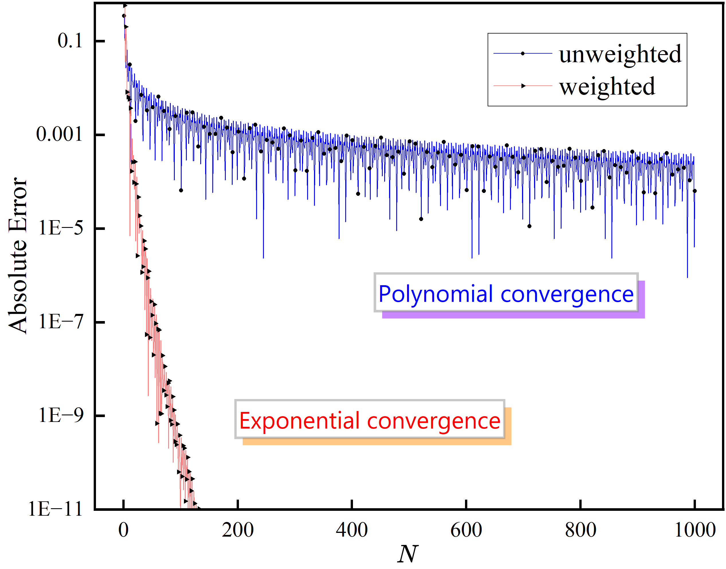
Under this setting, the unweighted multiple ergodic average (the multiple Birkhoff type) corresponds to

$${\frac{1}{N}\sum\limits_{n=0}^{N-1}{\sin\left({2\pi\left({\frac{1}{{10}}+\frac{{\sqrt{5}-1}}{2}n}\right)}\right)\sin\left({2\pi\left({\frac{1}{{10}}+n}\right)}\right)}},$$

and our weighted multiple ergodic average ${{\rm{DMW}}_{N}^{\ell}\left(\mathcal{F}\right)\left(\theta\right)}$ is expressed as

$${\frac{1}{{{A_{N}}}}\sum\limits_{n=0}^{N-1}{w\left({\frac{n}{N}}\right)\sin\left({2\pi\left({\frac{1}{{10}}+\frac{{\sqrt{5}-1}}{2}n}\right)}\right)\sin\left({2\pi\left({\frac{1}{{10}}+n}\right)}\right)}}.$$

As observed by Mondal et al in a recent work [40], oscillation around the mean is a universal behavior in such ergodic averages (at least for the unweighted type). In our case, both two averages oscillate around the mean $\prod\nolimits_{j=1}^{2}{\int_{{\mathbb{T}^{1}}}{{F_{j}}(\hat{\theta})d\hat{\theta}}}={\left({\int_{0}^{1}{\sin(2\pi\hat{\theta})d\hat{\theta}}}\right)^{2}}=0$. Therefore, we choose to calculate the absolute values of these two averages in Figure 1. As shown in Figure 1, our weighting method can improve the slow polynomial convergence (bule) into a rapid exponential convergence (red). In fact, the polynomial convergence rate of the unweighted type is $\mathcal{O}(N^{-1})$, either by co-boundary construction (see Katznelson [31] for instance) or by direct calculation.

6.2 The indispensability of the balancing conditions

In this subsection, we will demonstrate through numerical simulations that our balancing conditions are indispensable for achieving rapid convergence.

Refer to caption
Figure 2: The impact of regularity and irrationality on the convergence rates

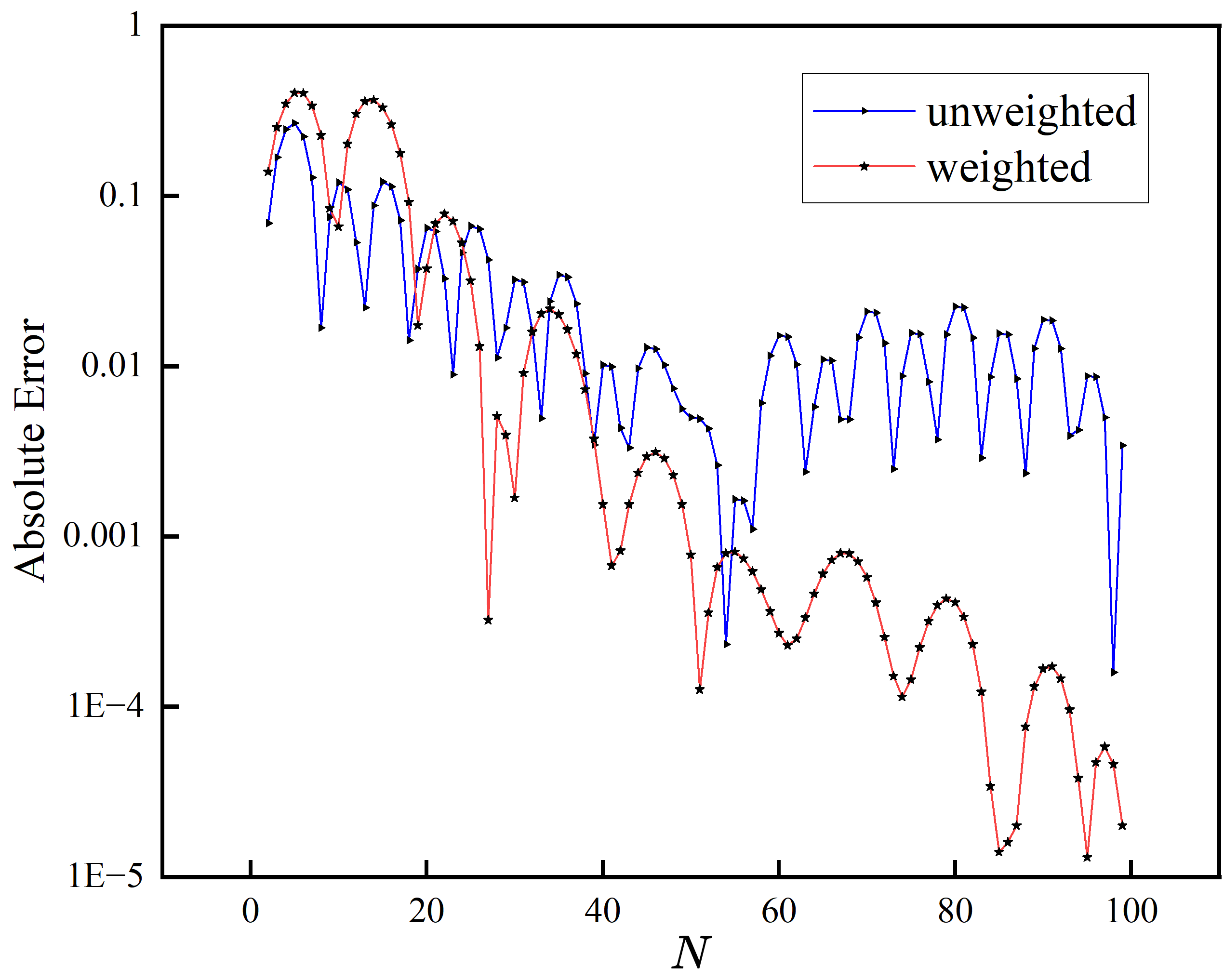
Our balancing conditions, namely (3.1), (3.4), (3.9) and (3.12), establish the effect of the regularity of the observables and the irrationality of the joint rotational vectors on the convergence rates. One may ask whether they are essential. Below we will construct a multiple example with weak regularity and weak irrationality and numerically simulate the convergence rates in Figure 2 to address this question: if our balancing conditions are not satisfied, the convergence rate may not be very fast.

Let the multiple index be $\ell=2$, the $1$-dimensional observables be

$${F_{1}}\left(x\right)=\sum\limits_{k=1}^{\infty}{\frac{1}{{{k^{2}}}}}\sin\left({2k\pi x}\right),{F_{2}}\left(x\right)=\sin\left({2\pi x}\right),$$

the rotations be ${\rho_{1}}=0.1001000100001\cdots$ and ${\rho_{2}}=1$, and the initial point be $\theta=10^{-1}$. One notices that $F_{1}(x)$ admits a regularity lower than $C^{2}(\mathbb{T}^{1})$, $F_{2}(x)$ is analytic, and $\rho_{1}$ is extremely Liouvillean (nearly rational). Then the joint nonresonant rotation becomes $\tilde{\rho}=\left({0.1001000100001\cdots,1}\right)$. It does not belong to any Diophantine class. Indeed, it is also extremely Liouvillean, because for any fixed $\gamma>0$ and $\tau>0$, there exists a subsequence ${\{{p_{{l_{s}}}},{q_{{l_{s}}}}\}_{s\in{\mathbb{N}^{+}}}}$ of the approximants ${\left\{{{p_{l}}/{q_{l}}}\right\}_{l\in{\mathbb{N}^{+}}}}$ of $\rho_{1}$, such that for infinitely many $k=\left({{k_{1}},{k_{2}}}\right)=\left({{p_{l_{s}}},0}\right)\in{\mathbb{Z}^{2}}$, it holds

$$\left|{k\cdot\tilde{\rho}-{q_{{l_{s}}}}}\right|=\left|{{p_{{l_{s}}}}{\rho_{1}}-{q_{{l_{s}}}}}\right|<\frac{\gamma}{{\left|{p_{{l_{s}}}}\right|^{\tau}}}=\frac{\gamma}{{{{\left|k\right|}^{\tau}}}},$$

which proves the claim. For simplicity, we do not give a specific expression of the averages as we did in Subsection 6.1. It is evident that the balancing condition (3.1) does not hold for any $m\in\mathbb{N}^{+}$, and one naturally expects a relatively slower rate of convergence for the multiple weighted average (although faster than the unweighted type).

Figure 2 illustrates this phenomenon. To ensure accuracy in the calculation, we utilize the Fourier series of $F_{1}(x)$ with $100$ terms and truncate $\rho_{1}$ to $0.010010001$. It is evident that the convergence rate of the weighted multiple average is still faster than that of the unweighted one, but significantly slower than the more regular and irrational case constructed in Subsection 6.1. For instance, for $N=100$, the error here is close to $10^{-5}$, whereas in Figure 2, the error is close to $10^{-11}$.

7 Proof of the abstract main results

This section is devoted to proving the abstract main results. It should be pointed out that the analysis of the continuous case $\mathrm{CMW}_{T}^{\ell}$ is much easier compared to the discrete case $\mathrm{DMW}_{N}^{\ell}$, as direct integration by parts can be utilized without the need for the Poisson summation formula. Hence, we have omitted the proof in this paper.

7.1 Arbitrary polynomial convergence in the finite-dimensional case: Proof of Theorem 3.1

Let us first consider the discrete case (3.2). Throughout the subsequent discussion, let $C_{1}>0$ denote a generic constant independent of $N$, which may vary in the context. We stress that $C_{1}$ is also independent of the dimension $d$ thanks to the boundedness condition (3.1) we have proposed.

With (2.7), we obtain that

$\displaystyle{F_{1}}\left({\mathscr{T}_{{\rho_{1}}}^{n}\left(\theta\right)}\right)\cdots{F_{\ell}}\left({\mathscr{T}_{{\rho_{\ell}}}^{n}\left(\theta\right)}\right)$
$\displaystyle=$ $\displaystyle\prod\limits_{j=1}^{\ell}{\left({\sum\limits_{{k^{j}}\in{\mathbb{Z}^{d}}}{{{({{\hat{F}}_{j}})}_{{k^{j}}}}{e^{2\pi i{k^{j}}\cdot\left({\theta+n{\rho_{j}}}\right)}}}}\right)}$
$\displaystyle=$ $\displaystyle\prod\limits_{j=1}^{\ell}{\left({\int_{{\mathbb{T}^{d}}}{{F_{j}}(\hat{\theta})d\hat{\theta}}}\right)}+\sum\limits_{0\neq{k^{1}},\ldots,{k^{\ell}}\in\mathbb{Z}^{d}}{\left({\prod\limits_{j=1}^{\ell}{{{({{\hat{F}}_{j}})}_{{k^{j}}}}}}\right)\exp\left({2\pi i\left({\sum\nolimits_{j=1}^{\ell}{{k^{j}}\cdot\theta}+n\sum\nolimits_{j=1}^{\ell}{{k^{j}}\cdot{\rho_{j}}}}\right)}\right)}.$ (7.1)

Next, we need to address the challenges arising from small divisors. For the fixed number ${\left({\sum\nolimits_{j=1}^{\ell}{{k^{j}}}}\right)\cdot\tilde{\rho}}$, denote by $\tilde{n}\in\mathbb{N}$ the closest integer to it. Note that $\tilde{n}$ is unique due to our Finite-dimensional joint nonresonant condition proposed in Definition 2.4. On the one hand, we have

$\displaystyle{\left|{\sum\nolimits_{j=1}^{\ell}{{k^{j}}\cdot{\rho_{j}}}-\tilde{n}}\right|^{-m}}$ $\displaystyle={\left|{\left({\sum\nolimits_{j=1}^{\ell}{{k^{j}}}}\right)\cdot\tilde{\rho}-\tilde{n}}\right|^{-m}}$
$\displaystyle\leqslant{\alpha^{-m}}{\Delta^{m}}\left({\left\|{\sum\nolimits_{j=1}^{\ell}{{k^{j}}}}\right\|}\right)$
$\displaystyle\equiv{\alpha^{-m}}{\Delta^{m}}\left({\sum\nolimits_{j=1}^{\ell}{\left\|{{k^{j}}}\right\|}}\right).$ (7.2)

On the other hand, with $m\geqslant 2$ we have

$$\sum\limits_{\tilde{n}\neq n\in\mathbb{Z}}{{{\left|{\sum\nolimits_{j=1}^{\ell}{{k^{j}}\cdot{\rho_{j}}}-n}\right|}^{-m}}}\leqslant 2\sum\limits_{n=0}^{+\infty}{{{\left({n+{2^{-1}}}\right)}^{-m}}}\leqslant 2\sum\limits_{n=0}^{+\infty}{{{\left({n+{2^{-1}}}\right)}^{-2}}}<10.$$ (7.3)

Note that $\left\|{\sum\nolimits_{j=1}^{\ell}{{k^{j}}}}\right\|\geqslant 1$ since $\sum\nolimits_{j=1}^{\ell}{{k^{j}}}=\left({{k^{1}},\ldots,{k^{\ell}}}\right)\in{\mathbb{Z}^{d\ell}}\backslash\left\{0\right\}$, and ${\Delta^{m}}\left(1\right)=1$. We therefore obtain that

$\displaystyle\sum\limits_{n=-\infty}^{+\infty}{{{\left|{\sum\nolimits_{j=1}^{\ell}{{k^{j}}\cdot{\rho_{j}}}-n}\right|}^{-m}}}$ $\displaystyle={\left|{\sum\nolimits_{j=1}^{\ell}{{k^{j}}\cdot{\rho_{j}}}-\tilde{n}}\right|^{-m}}+\sum\limits_{\tilde{n}\neq n\in\mathbb{Z}}{{{\left|{\sum\nolimits_{j=1}^{\ell}{{k^{j}}\cdot{\rho_{j}}}-n}\right|}^{-m}}}$
$\displaystyle\leqslant{C_{1}}{\Delta^{m}}\left({\sum\nolimits_{j=1}^{\ell}{\left\|{{k^{j}}}\right\|}}\right).$

This leads to

$\displaystyle\sum\limits_{n=-\infty}^{+\infty}{\left|{\int_{0}^{1}{w\left(y\right)\exp\left({2\pi iNy\left({\sum\nolimits_{j=1}^{\ell}{{k^{j}}\cdot{\rho_{j}}}-n}\right)}\right)dy}}\right|}$
$\displaystyle\leqslant$ $\displaystyle{\left({2\pi N}\right)^{-m}}{\left\|{{w^{\left(m\right)}}}\right\|_{{L^{1}}\left({0,1}\right)}}\sum\limits_{n=-\infty}^{+\infty}{{{\left|{\sum\nolimits_{j=1}^{\ell}{{k^{j}}\cdot{\rho_{j}}}-n}\right|}^{-m}}}$ (7.4)
$\displaystyle\leqslant$ $\displaystyle{C_{1}}{N^{-m}}{\Delta^{m}}\left({\sum\nolimits_{j=1}^{\ell}{\left\|{{k^{j}}}\right\|}}\right)$ (7.5)

by integrating by parts since $w\in C_{0}^{\infty}([0,1])$, where the following trivial estimate is used

$${\left|{\int_{0}^{1}{{w^{\left(m\right)}}\left(y\right)\exp\left({2\pi iNy\left({\sum\nolimits_{j=1}^{\ell}{{k^{j}}\cdot{\rho_{j}}}-n}\right)}\right)dy}}\right|}\leqslant{\left\|{{w^{\left(m\right)}}}\right\|_{{L^{1}}\left({0,1}\right)}}.$$ (7.6)

At this time, with the help of (7.5) and the Poisson summation formula in Lemma 8.1, we arrive at the estimates below due to $w\in C_{0}^{\infty}([0,1])$:

$\displaystyle\left|{{N^{-1}}\sum\limits_{n=0}^{N-1}{w\left({n/N}\right)\exp\left({2\pi in\sum\nolimits_{j=1}^{\ell}{{k^{j}}\cdot{\rho_{j}}}}\right)}}\right|$
$\displaystyle=$ $\displaystyle\left|{{N^{-1}}\sum\limits_{n=-\infty}^{+\infty}{w\left({n/N}\right)\exp\left({2\pi in\sum\nolimits_{j=1}^{\ell}{{k^{j}}\cdot{\rho_{j}}}}\right)}}\right|$
$\displaystyle=$ $\displaystyle\left|{{N^{-1}}\sum\limits_{n=-\infty}^{+\infty}{\int_{-\infty}^{+\infty}{w\left({t/N}\right)\exp\left({2\pi it\left({\sum\nolimits_{j=1}^{\ell}{{k^{j}}\cdot{\rho_{j}}}-n}\right)}\right)dt}}}\right|$
$\displaystyle=$ $\displaystyle\left|{{N^{-1}}\sum\limits_{n=-\infty}^{+\infty}{\int_{0}^{N}{w\left({t/N}\right)\exp\left({2\pi it\left({\sum\nolimits_{j=1}^{\ell}{{k^{j}}\cdot{\rho_{j}}}-n}\right)}\right)dt}}}\right|$
$\displaystyle\leqslant$ $\displaystyle\sum\limits_{n=-\infty}^{+\infty}{\left|{\int_{0}^{1}{w\left(y\right)\exp\left({2\pi iNy\left({\sum\nolimits_{j=1}^{\ell}{{k^{j}}\cdot{\rho_{j}}}-n}\right)}\right)dy}}\right|}$
$\displaystyle\leqslant$ $\displaystyle{C_{1}}{N^{-m}}{\Delta^{m}}\left({\sum\nolimits_{j=1}^{\ell}{\left\|{{k^{j}}}\right\|}}\right).$ (7.7)

Now, building upon the previous preparations and

$$\frac{N}{{{A_{N}}}}={\left({\frac{1}{N}\sum\limits_{s=0}^{N-1}{w\left({s/N}\right)}}\right)^{-1}}\to{\left({\int_{0}^{1}{w\left(x\right)dx}}\right)^{-1}}>0,$$

one can derive the promised polynomial convergence (of order $m$) as

$\displaystyle{\left\|{\mathrm{DMW}_{N}^{\ell}\left(\mathcal{F}\right)\left(\theta\right)-\prod\limits_{j=1}^{\ell}{\left({\int_{{\mathbb{T}^{d}}}{{F_{j}}(\hat{\theta})d\hat{\theta}}}\right)}}\right\|_{\mathscr{B}}}$
$\displaystyle=$ $\displaystyle{\left\|{\frac{1}{{{A_{N}}}}\sum\limits_{n=0}^{N-1}{w\left({n/N}\right)\sum\limits_{0\neq{k^{1}},\ldots,{k^{\ell}}\in{\mathbb{Z}^{d}}}{\left({\prod\limits_{j=1}^{\ell}{{{({{\hat{F}}_{j}})}_{{k^{j}}}}}}\right)\exp\left({2\pi i\left({\sum\nolimits_{j=1}^{\ell}{{k^{j}}\cdot\theta}+n\sum\nolimits_{j=1}^{\ell}{{k^{j}}\cdot{\rho_{j}}}}\right)}\right)}}}\right\|_{\mathscr{B}}}$ (7.8)
$\displaystyle\leqslant$ $\displaystyle\frac{C_{1}N}{{{A_{N}}}}\sum\limits_{0\neq{k^{1}},\ldots,{k^{\ell}}\in{\mathbb{Z}^{d}}}{\frac{1}{{\prod\nolimits_{j=1}^{\ell}{{{\tilde{\Delta}}_{j}}\left({\left\|{{k^{j}}}\right\|}\right)}}}\left|{{N^{-1}}\sum\limits_{n=0}^{N-1}{w\left({n/N}\right)\exp\left({2\pi in\sum\nolimits_{j=1}^{\ell}{{k^{j}}\cdot{\rho_{j}}}}\right)}}\right|}$ (7.9)
$\displaystyle\leqslant$ $\displaystyle{C_{1}}{N^{-m}}\sum\limits_{0\neq{k^{1}},\ldots,{k^{\ell}}\in{\mathbb{Z}^{d}}}{\frac{{{\Delta^{m}}\left({\sum\nolimits_{j=1}^{\ell}{\left\|{{k^{j}}}\right\|}}\right)}}{{\prod\nolimits_{j=1}^{\ell}{{{\tilde{\Delta}}_{j}}\left({\left\|{{k^{j}}}\right\|}\right)}}}}$ (7.10)
$\displaystyle=$ $\displaystyle\mathcal{O}\left({{N^{-m}}}\right).$ (7.11)

Here (7.8) uses (7.5), (7.9) is because $F_{j}\in\mathscr{B}_{\tilde{\Delta}_{j}}$ for $1\leqslant j\leqslant\ell$, (7.10) uses (7.7), and finally (7.11) follows from the boundedness condition (3.1). This gives the proof of the discrete case (3.2), i.e., the polynomial convergence $\mathcal{O}\left({{N^{-m}}}\right)$ of the multiple ergodic average $\mathrm{DMW}_{N}^{\ell}$.

Given that the proof of the continuous case (3.3) follows a similar structure to the one presented above and is, in fact, simpler, we can conclude the proof of Theorem 3.1.

7.2 Arbitrary polynomial convergence in the infinite-dimensional case: Proof of Theorem 3.2

The proof closely resembles that of Theorem 3.1, with the key observation being that the universal constant is dimension-independent, as indicated in Comment (C3).

7.3 Exponential convergence in the finite-dimensional case: Proof of Theorem 3.3

It suffices to show the proof of the discrete case (3.10). Firstly, note that

$\displaystyle\left|{{N^{-1}}\sum\limits_{n=0}^{N-1}{w\left({n/N}\right)\exp\left({2\pi in\sum\nolimits_{j=1}^{\ell}{{k^{j}}\cdot{\rho_{j}}}}\right)}}\right|$
$\displaystyle\leqslant$ $\displaystyle{N^{-1}}\sum\limits_{n=0}^{N-1}{w\left({n/N}\right)}\to\int_{0}^{1}{w\left(x\right)dx}=1.$

Building upon the proof of Theorem 3.1 and the definition of the truncated space $\mathscr{S}(x)$ in (3.7), one derives that

$\displaystyle{\left\|{\mathrm{DMW}_{N}^{\ell}\left(F\right)\left(\theta\right)-\prod\limits_{j=1}^{\ell}{\left({\int_{{\mathbb{T}^{d}}}{{F_{j}}(\hat{\theta})d\hat{\theta}}}\right)}}\right\|_{\mathscr{B}}}$
$\displaystyle\leqslant{\tilde{C}_{1}}\sum\limits_{0\neq{k^{1}},\ldots,{k^{\ell}}\in{\mathbb{Z}^{d}}}{\frac{1}{{\prod\nolimits_{j=1}^{\ell}{{{\tilde{\Delta}}_{j}}\left({\left\|{{k^{j}}}\right\|}\right)}}}\left|{{N^{-1}}\sum\limits_{n=0}^{N-1}{w\left({n/N}\right)\exp\left({2\pi in\sum\nolimits_{j=1}^{\ell}{{k^{j}}\cdot{\rho_{j}}}}\right)}}\right|}$
$\displaystyle\leqslant{{\tilde{C}}_{1}}\sum\limits_{0\neq\sum\nolimits_{j=1}^{\ell}{{k^{j}}}\in\mathscr{S}\left(N\right)}{\frac{{\mathcal{I}\left({N,\left\{{{k^{j}}}\right\}_{j=1}^{\ell},\left\{{{\rho_{j}}}\right\}_{j=1}^{\ell}}\right)}}{{\prod\nolimits_{j=1}^{\ell}{{{\tilde{\Delta}}_{j}}\left({\left\|{{k^{j}}}\right\|}\right)}}}}$
$\displaystyle\;\;\;\;+{{\tilde{C}}_{1}}\sum\limits_{0\neq\sum\nolimits_{j=1}^{\ell}{{k^{j}}}\in{\mathbb{Z}^{d\ell}}\backslash\mathscr{S}\left(N\right)}{\frac{1}{{\prod\nolimits_{j=1}^{\ell}{{{\tilde{\Delta}}_{j}}\left({\left\|{{k^{j}}}\right\|}\right)}}}}$
$\displaystyle:={\tilde{C}_{1}}\left({{\mathcal{J}_{1}}+{\mathcal{J}_{2}}}\right),$ (7.12)

where the constant $\tilde{C}_{1}$ is independent of the parameter $m$ (the finite degree of integration by parts) in Theorem 3.1, and we denote

$\displaystyle\mathcal{I}\left({N,\left\{{{k^{j}}}\right\}_{j=1}^{\ell},\left\{{{\rho_{j}}}\right\}_{j=1}^{\ell}}\right)$
$\displaystyle:=$ $\displaystyle\sum\limits_{n=-\infty}^{+\infty}{\left|{\int_{0}^{1}{w\left(y\right)\exp\left({2\pi iNy\left({\sum\nolimits_{j=1}^{\ell}{{k^{j}}\cdot{\rho_{j}}}-n}\right)}\right)dy}}\right|}$ (7.13)

in ${\mathcal{J}_{1}}$ for convenience.

Next we provide a summary of our strategy. In view of (7.12), we will do different operations for $\mathcal{J}_{1}$ and $\mathcal{J}_{2}$. For the former, we consider letting the time of integration by parts (specifically $\mathcal{K}(N)$ chosen below) vary, i.e., adapting it based on $N$ and the adaptive function $\varphi$ which appears in the truncated space $\mathscr{S}(x)$. This approach is expected to yield an exponential estimate for $\mathcal{J}_{1}$. As for the latter, the truncated smallness condition (3.9) implies that $\mathcal{J}_{2}$ is automatically exponentially small. By combining these two parts one could complete the proof. The details are given below.

On the one hand, for the absolute constant $\beta>0$ in Lemma 8.2, there exist $\bar{\beta}>\beta$ and some $\beta_{1}>0$ such that the following holds with $N$ sufficiently large:

$${\left({\frac{{{\mathcal{K}^{\beta}}\left(N\right)}}{{2\pi\alpha\varphi\left(N\right)}}}\right)^{\mathcal{K}\left(N\right)}}\leqslant{\left({\frac{{{\mathcal{K}^{\bar{\beta}}}\left(N\right)}}{{\varphi\left(N\right)}}}\right)^{\mathcal{K}\left(N\right)}}=\mathcal{O}\left({\exp\left({-{\varphi^{{\beta_{1}}}}\left(N\right)}\right)}\right),$$

where $\mathcal{K}\left(N\right)=\left[{{e^{-1}}{\varphi^{{{\bar{\beta}}^{-1}}}}\left(N\right)}\right]\geqslant 2$ due to $\varphi(+\infty)=+\infty$ (note that $\varphi$ is an adaptive function, see Definition 2.2). Recall (7.2), (7.3) and (7.4). Consequently, for $0\neq\sum\nolimits_{j=1}^{\ell}{{k^{j}}}\in\mathscr{S}\left(N\right)$ we have

$\displaystyle\mathcal{I}\left({N,\left\{{{k^{j}}}\right\}_{j=1}^{\ell},\left\{{{\rho_{j}}}\right\}_{j=1}^{\ell}}\right)$
$\displaystyle=$ $\displaystyle{\left({2\pi N}\right)^{-\mathcal{K}\left(N\right)}}{\left\|{{w^{\left({\mathcal{K}\left(N\right)}\right)}}}\right\|_{{L^{1}}\left({0,1}\right)}}\left({\sum\limits_{n=-\infty}^{+\infty}{{{\left|{\sum\nolimits_{j=1}^{\ell}{{k^{j}}\cdot{\rho_{j}}-n}}\right|}^{-\mathcal{K}\left(N\right)}}}}\right)$ (7.14)
$\displaystyle\leqslant$ $\displaystyle{\left({2\pi N}\right)^{-\mathcal{K}\left(N\right)}}{\left({\mathcal{K}\left(N\right)}\right)^{\mathcal{K}\left(N\right)\beta}}\left({{\alpha^{-\mathcal{K}\left(N\right)}}{\Delta^{\mathcal{K}\left(N\right)}}\left({\left\|{\sum\nolimits_{j=1}^{\ell}{{k^{j}}}}\right\|}\right)}\right)$
$\displaystyle\equiv$ $\displaystyle{\left({\frac{{{\mathcal{K}^{\beta}}\left(N\right)}}{{2\pi\alpha N}}}\right)^{\mathcal{K}\left(N\right)}}\left({{\Delta^{\mathcal{K}\left(N\right)}}\left({\sum\nolimits_{j=1}^{\ell}{\left\|{{k^{j}}}\right\|}}\right)}\right)$
$\displaystyle\leqslant$ $\displaystyle{\left({\frac{{{\mathcal{K}^{\beta}}\left(N\right)}}{{2\pi\alpha N}}}\right)^{\mathcal{K}\left(N\right)}}\left({{\Delta^{\mathcal{K}\left(N\right)}}\left({\sum\nolimits_{j=1}^{\ell}{{\ell^{-1}}{\Delta^{-1}}\left({N/\varphi\left(N\right)}\right)}}\right)}\right)$
$\displaystyle=$ $\displaystyle{\left({\frac{{{\mathcal{K}^{\beta}}\left(N\right)}}{{2\pi\alpha\varphi\left(N\right)}}}\right)^{\mathcal{K}\left(N\right)}}$
$\displaystyle=$ $\displaystyle\mathcal{O}\left({\exp\left({-{\varphi^{{\beta_{1}}}}\left(N\right)}\right)}\right).$ (7.15)

This leads to the estimates for $\mathcal{J}_{1}$ below:

$\displaystyle{\mathcal{J}_{1}}$ $\displaystyle=\sum\limits_{0\neq\sum\nolimits_{j=1}^{\ell}{{k^{j}}}\in\mathscr{S}\left(N\right)}{\frac{{\mathcal{I}\left({N,\left\{{{k^{j}}}\right\}_{j=1}^{\ell},\left\{{{\rho_{j}}}\right\}_{j=1}^{\ell}}\right)}}{{\prod\nolimits_{j=1}^{\ell}{{{\tilde{\Delta}}_{j}}\left({\left\|{{k^{j}}}\right\|}\right)}}}}$
$\displaystyle=\sum\limits_{0\neq\sum\nolimits_{j=1}^{\ell}{{k^{j}}}\in\mathscr{S}\left(N\right)}{\frac{{\mathcal{O}\left({\exp\left({-{\varphi^{{\beta_{1}}}}\left(N\right)}\right)}\right)}}{{\prod\nolimits_{j=1}^{\ell}{{{\tilde{\Delta}}_{j}}\left({\left\|{{k^{j}}}\right\|}\right)}}}}$
$\displaystyle=\mathcal{O}\left(\sum\limits_{0\neq{k^{1}},\ldots,{k^{\ell}}\in{\mathbb{Z}^{d}}}{\frac{1}{{\prod\nolimits_{j=1}^{\ell}{{{\tilde{\Delta}}_{j}}\left({\left\|{{k^{j}}}\right\|}\right)}}}}\right)\cdot\mathcal{O}\left({\exp\left({-{\varphi^{{\beta_{1}}}}\left(N\right)}\right)}\right)$
$\displaystyle=\mathcal{O}\left({\exp\left({-{\varphi^{{\beta_{1}}}}\left(N\right)}\right)}\right),$ (7.16)

where the truncated smallness condition (3.9) is applied in (7.16) due to Cauchy’s Theorem, as shown in Comment (C1).

On the other hand, in view of the truncated smallness condition (3.9), we directly get

$${\mathcal{J}_{2}}=\sum\limits_{0\neq\sum\nolimits_{j=1}^{\ell}{{k^{j}}}\in{\mathbb{Z}^{d\ell}}\backslash\mathscr{S}\left(N\right)}{\frac{1}{{\prod\nolimits_{j=1}^{\ell}{{{\tilde{\Delta}}_{j}}\left({\left\|{{k^{j}}}\right\|}\right)}}}}=\mathcal{O}\left({{e^{-cN}}}\right).$$ (7.17)

Substituting (7.16) and (7.17) into (7.12) and comparing the order, we finally arrive at the desired exponential convergence for the multiple ergodic average $\mathrm{DMW}_{N}^{\ell}$:

$${\left\|{\mathrm{DMW}_{N}^{\ell}\left(\mathcal{F}\right)\left(\theta\right)-\prod\limits_{j=1}^{\ell}\left({\int_{{\mathbb{T}^{d}}}{{F_{j}}(\hat{\theta})d\hat{\theta}}}\right)}\right\|_{\mathscr{B}}}=\mathcal{O}\left(\exp(-\varphi^{\beta_{1}}(N))\right),$$

because the adaptive function $\varphi$ satisfies $\varphi(x)=o(x)$, as defined in Definition 2.2.

As to the continuous case (3.11), the proof is similar since one does not have to apply the Poisson summation formula. We therefore finish the proof of Theorem 3.3.

7.4 Exponential convergence in the infinite-dimensional case: Proof of Theorem 3.4

The proof closely resembles that of Theorem 3.3, with the key observation being that the universal constant is dimension-independent, as indicated in Comment (C3) due to our truncated smallness condition (3.12).

7.5 Exponential convergence via trigonometric polynomials: Proof of Theorem 3.5

We only show the proof for the discrete case (3.13) with $d<+\infty$. Denote by $C_{2}>0$ a universal constant independent of $N$. With the analysis in Section 7.3 in mind, one verifies that

$$\sum\limits_{n=-\infty}^{+\infty}{{{\left|{\sum\nolimits_{j=1}^{\ell}{{k^{j}}\cdot{\rho_{j}}-n}}\right|}^{-\tilde{\mathcal{K}}\left(N\right)}}}\leqslant{C_{2}}$$

since $0\neq\|k^{j}\|\leqslant K$. Choose $\tilde{\mathcal{K}}\left(N\right)=\left[{{e^{-1}}{{\left({C_{2}^{-1}N}\right)}^{1/\beta}}}\right]\geqslant 2$. Then it follows from (7.13) and (7.14) that

$\displaystyle\mathcal{I}\left({N,\left\{{{k^{j}}}\right\}_{j=1}^{\ell},\left\{{{\rho_{j}}}\right\}_{j=1}^{\ell}}\right)$
$\displaystyle\leqslant$ $\displaystyle{\left({2\pi N}\right)^{-\tilde{\mathcal{K}}\left(N\right)}}{\left({\tilde{\mathcal{K}}\left(N\right)}\right)^{\tilde{\mathcal{K}}\left(N\right)\beta}}\left({\sum\limits_{n=-\infty}^{+\infty}{{{\left|{\sum\nolimits_{j=1}^{\ell}{{k^{j}}\cdot{\rho_{j}}-n}}\right|}^{-{\mathcal{K}}\left(N\right)}}}}\right)$
$\displaystyle\leqslant$ $\displaystyle{\left({{C_{2}}{N^{-1}}{{\tilde{\mathcal{K}}}^{\beta}}\left(N\right)}\right)^{\tilde{\mathcal{K}}\left(N\right)}}$
$\displaystyle=$ $\displaystyle\mathcal{O}\left({\exp\left({{N^{-\hat{c}}}}\right)}\right)$ (7.18)

with some $\hat{c}>0$, in other words, we obtain a better convergence rate than that in (7.15) under the trigonometric polynomial setting. One finally arrives at the followings by (7.18):

$\displaystyle{\left\|{\mathrm{DMW}_{N}^{\ell}\left(\mathcal{F}\right)\left(\theta\right)-\prod\limits_{j=1}^{\ell}{\left({\int_{{\mathbb{T}^{1}}}{{F_{j}}(\hat{\theta})d\hat{\theta}}}\right)}}\right\|_{\mathscr{B}}}$
$\displaystyle=$ $\displaystyle\mathcal{O}\left({\sum\limits_{0\neq|{k^{\iota}}|\leqslant K,1\leqslant\iota\leqslant j}{\frac{{\mathcal{I}\left({N,\left\{{{k^{j}}}\right\}_{j=1}^{\ell},\left\{{{\rho_{j}}}\right\}_{j=1}^{\ell}}\right)}}{{\prod\nolimits_{j=1}^{\ell}{{{\tilde{\Delta}}_{j}}\left({\left|{{k^{j}}}\right|}\right)}}}}}\right)$
$\displaystyle=$ $\displaystyle\mathcal{O}\left({\sum\limits_{0\neq|{k^{\iota}}|\leqslant K,1\leqslant\iota\leqslant j}{\frac{1}{{\prod\nolimits_{j=1}^{\ell}{{{\tilde{\Delta}}_{j}}\left({\left|{{k^{j}}}\right|}\right)}}}}}\right)\cdot\mathcal{O}\left({\exp\left({{N^{-\hat{c}}}}\right)}\right)$
$\displaystyle=$ $\displaystyle\mathcal{O}\left({\exp\left({{N^{-\hat{c}}}}\right)}\right).$

This demonstrates the exponential convergence. As to the continuous case (3.14), the proof is similar and we therefore omit here.

For the continuous case with $d=1$, i.e., (3.15), we only have to notice that

$$\sum\limits_{0\neq{k^{1}},\ldots,{k^{\ell}}\in\mathbb{Z}}{\frac{1}{{\prod\nolimits_{j=1}^{\ell}{{{\tilde{\Delta}}_{j}}\left({\left|{{k^{j}}}\right|}\right)}}}}=\mathcal{O}\left({\prod\limits_{j=1}^{\ell}{\left({\int_{1}^{+\infty}{\frac{1}{{{{\tilde{\Delta}}_{j}}\left(x\right)}}dx}}\right)}}\right)=\mathcal{O}\left(1\right)$$

thanks to (3.16), then the proof is also similar since the universal coefficient is bounded, and the estimates obtained by integration by parts are exponentially small via the finite nonresonant assumptions, namely $\sum\nolimits_{j=1}^{\ell}{{k^{j}}{\rho_{j}}}\neq 0$ hold for all $0<\left\|{{k^{j}}}\right\|\leqslant K$. This proves Theorem 3.5.

8 Appendix

Lemma 8.1 (Poisson summation formula).

For each $h\left(x\right)\in\mathcal{C}\left(\mathbb{R}\right)$ (the Schwartz space), there holds

$$\sum\limits_{n\in\mathbb{Z}}{h\left(n\right)}=\sum\limits_{n\in\mathbb{Z}}{\int_{-\infty}^{+\infty}{h\left(x\right){e^{-2\pi nix}}dx}}.$$
Proof.

See Chapter 3 in [24] for details. ∎

Lemma 8.2.

Define the weighting function as

$$w\left(x\right)=\exp\left({-{x^{-1}}{{\left({1-x}\right)}^{-1}}}\right)\cdot{\left({\int_{0}^{1}{\exp\left({-{t^{-1}}{{\left({1-t}\right)}^{-1}}}\right)dt}}\right)^{-1}}$$

on $(0,1)$. Then there exists $\beta>1$ such that

$${\left\|{{w^{\left(n\right)}}}\right\|_{{L^{1}}\left({0,1}\right)}}=\mathcal{O}\left({{n^{n\beta}}}\right),\;\;n\to+\infty.$$ (8.1)
Proof.

See Lemma 5.3 in [49] for details. ∎

Lemma 8.3.

For any given $\rho_{*}>0$ and $\mu\in{\mathbb{N}^{+}}$, there exists $\tau=\tau\left({\eta,\mu}\right)>0$ such that

$$\prod\limits_{j\in\mathbb{N}}{\left({1+{{\left|{{k_{j}}}\right|}^{\mu}}{{\left\langle j\right\rangle}^{\mu}}}\right)}\leqslant\exp\left({\frac{\tau}{{{\rho_{*}^{1/\eta}}}}\log\left({\frac{\tau}{\rho_{*}}}\right)}\right)\cdot{e^{\rho_{*}{{\left|k\right|}_{\eta}}}}.$$
Proof.

See details in Lemma B.1 in [41] and Lemma 7.2 in [6]. ∎

Lemma 8.4.

For $2\leqslant\eta\in{\mathbb{N}^{+}}$, the following holds whenever $\nu\in\mathbb{N}^{+}$ is sufficiently large:

$$\sum\limits_{0\neq k\in\mathbb{Z}_{*}^{\infty},{{\left|k\right|}_{\eta}}=\nu}1:=\#\left\{{k:0\neq k\in\mathbb{Z}_{*}^{\infty},{{\left|k\right|}_{\eta}}=\nu\in{\mathbb{N}^{+}}}\right\}=\mathcal{O}\left({\nu^{{\nu^{1/\eta}}}}\right).$$ (8.2)
Proof.

Recall that

$${\left|k\right|_{\eta}}=\sum\limits_{j\in\mathbb{N}}{{{\left\langle j\right\rangle}^{\eta}}\left|{{k_{j}}}\right|}\in{\mathbb{N}^{+}}.$$

Then the largest non-zero integer ${j_{\max}}$ in (8.2) satisfies that ${j_{\max}}\leqslant\left[{{\nu^{1/\eta}}}\right]$. Therefore,

$\displaystyle\#\left\{{k:0\neq k\in\mathbb{Z}_{*}^{\infty},{{\left|k\right|}_{\eta}}=\nu\in{\mathbb{N}^{+}}}\right\}$
$\displaystyle\leqslant$ $\displaystyle\#\left\{{k:0\neq k\in\mathbb{Z}_{*}^{\infty},|{k_{0}}|+|{k_{1}}|+\cdots+|{k_{\left[{{\nu^{1/\eta}}}\right]}}|=\nu\in{\mathbb{N}^{+}}}\right\}$
$\displaystyle\leqslant$ $\displaystyle{2^{\left[{{\nu^{1/\eta}}}\right]+1}}\cdot\#\left\{{k:0\neq k\in\mathbb{Z}_{*}^{\infty},\text{${k_{j}}\in\mathbb{N}$ for all $j\in\mathbb{N}$},{k_{0}}+{k_{1}}+\cdots+{k_{\left[{{\nu^{1/\eta}}}\right]}}=\nu\in{\mathbb{N}^{+}}}\right\}$
$\displaystyle=$ $\displaystyle{2^{\left[{{\nu^{1/\eta}}}\right]+1}}\cdot C_{\nu+\left[{{\nu^{1/\eta}}}\right]}^{\nu}$
$\displaystyle\leqslant$ $\displaystyle{2^{\left[{{\nu^{1/\eta}}}\right]+1}}\cdot{C_{\eta}}\frac{1}{{\sqrt{{\nu^{1/\eta}}}}}\cdot{\nu^{\left({1-1/\eta}\right)\left({{\nu^{1/\eta}}+1}\right)}}\cdot{e^{\left[{{\nu^{1/\eta}}}\right]}}$ (8.3)
$\displaystyle\leqslant$ $\displaystyle{C_{\eta}}{\nu^{{\nu^{1/\eta}}}}.$

Here (8.3) uses the following fact, by applying the Stirling’s approximation $n!\sim\sqrt{2\pi n}{\left({n/e}\right)^{n}}$ as $n\to+\infty$:

$\displaystyle\;\;\;\;\;\;C_{\nu+\left[{{\nu^{1/\eta}}}\right]}^{\nu}$
$\displaystyle=\frac{{\left({\nu+\left[{{\nu^{1/\eta}}}\right]}\right)!}}{{\nu!\left({\left[{{\nu^{1/\eta}}}\right]}\right)!}}\sim\frac{{\sqrt{2\pi\left({\nu+\left[{{\nu^{1/\eta}}}\right]}\right)}{{\left({\frac{{\nu+\left[{{\nu^{1/\eta}}}\right]}}{e}}\right)}^{\nu+\left[{{\nu^{1/\eta}}}\right]}}}}{{\sqrt{2\pi\nu}{{\left({\frac{\nu}{e}}\right)}^{\nu}}\cdot\sqrt{2\pi\left[{{\nu^{1/\eta}}}\right]}{{\left({\frac{{\left[{{\nu^{1/\eta}}}\right]}}{e}}\right)}^{\left[{{\nu^{1/\eta}}}\right]}}}}$
$\displaystyle\sim\frac{1}{{\sqrt{2\pi{\nu^{1/\eta}}}}}\cdot{\left({1+\frac{{\left[{{\nu^{1/\eta}}}\right]}}{\nu}}\right)^{\nu}}\cdot{\left({\frac{\nu}{{\left[{{\nu^{1/\eta}}}\right]}}}\right)^{\left[{{\nu^{1/\eta}}}\right]}}\cdot{\left({1+\frac{{\left[{{\nu^{1/\eta}}}\right]}}{\nu}}\right)^{\left[{{\nu^{1/\eta}}}\right]}}$
$\displaystyle=\frac{1}{{\sqrt{2\pi{\nu^{1/\eta}}}}}\cdot{\left({\frac{\nu}{{\left[{{\nu^{1/\eta}}}\right]}}}\right)^{\left[{{\nu^{1/\eta}}}\right]}}\cdot\exp\left({\nu\log\left({1+\frac{{\left[{{\nu^{1/\eta}}}\right]}}{\nu}}\right)}\right)$
$\displaystyle\;\;\;\;\cdot\exp\left({\left[{{\nu^{1/\eta}}}\right]\log\left({1+\frac{{\left[{{\nu^{1/\eta}}}\right]}}{\nu}}\right)}\right)$
$\displaystyle=\frac{1}{{\sqrt{2\pi{\nu^{1/\eta}}}}}\cdot{\left({\frac{\nu}{{\left[{{\nu^{1/\eta}}}\right]}}}\right)^{\left[{{\nu^{1/\eta}}}\right]}}\cdot\exp\left({\nu\left({\frac{{\left[{{\nu^{1/\eta}}}\right]}}{\nu}-\frac{1}{2}\frac{{{{\left[{{\nu^{1/\eta}}}\right]}^{2}}}}{{{\nu^{2}}}}+\cdots}\right)}\right)$
$\displaystyle\;\;\;\;\cdot\exp\left({\left[{{\nu^{1/\eta}}}\right]\left({\frac{{\left[{{\nu^{1/\eta}}}\right]}}{\nu}+\cdots}\right)}\right)$
$\displaystyle=\frac{1}{{\sqrt{2\pi{\nu^{1/\eta}}}}}\cdot{\left({\frac{\nu}{{\left[{{\nu^{1/\eta}}}\right]}}}\right)^{\left[{{\nu^{1/\eta}}}\right]}}\cdot\exp\left({\left[{{\nu^{1/\eta}}}\right]-\frac{{{{\left[{{\nu^{1/\eta}}}\right]}^{2}}}}{{2\nu}}+\cdots}\right)\cdot\exp\left({\frac{{{{\left[{{\nu^{1/\eta}}}\right]}^{2}}}}{\nu}+\cdots}\right)$
$\displaystyle=\frac{1}{{\sqrt{2\pi{\nu^{1/\eta}}}}}\cdot{\left({\frac{\nu}{{\left[{{\nu^{1/\eta}}}\right]}}}\right)^{\left[{{\nu^{1/\eta}}}\right]}}\cdot\exp\left({\left[{{\nu^{1/\eta}}}\right]+\mathcal{O}\left(1\right)}\right)\cdot\exp\left({\mathcal{O}\left(1\right)}\right)(\text{since $\eta\geqslant 2$})$
$\displaystyle\leqslant{C_{\eta}}\frac{1}{{\sqrt{{\nu^{1/\eta}}}}}\cdot{\nu^{\left({1-1/\eta}\right)\left({{\nu^{1/\eta}}+1}\right)}}\cdot{e^{\left[{{\nu^{1/\eta}}}\right]}}.$

This proves the lemma. ∎

Lemma 8.5.

Let $\zeta>0,\ell\in\mathbb{N}^{+}$ and $\left\{{{a_{j}}}\right\}_{j=1}^{\ell}>0$ be given. Then there exists a constant $C\left({\zeta,\ell}\right)>0$ such that

$${\left({\sum\nolimits_{j=1}^{\ell}{{a_{j}}}}\right)^{\zeta}}\leqslant C\left({\zeta,\ell}\right)\left({\sum\nolimits_{j=1}^{\ell}{a_{j}^{\zeta}}}\right).$$
Proof.

It suffices to prove the conclusion for $\ell\geqslant 2$. For $\ell=2$, denote ${b_{j}}={\left({\sum\nolimits_{s=1}^{2}{{a_{s}}}}\right)^{-1}}{a_{j}}$ with $1\leqslant j\leqslant 2$. This leads to $\sum\nolimits_{j=1}^{2}{{b_{j}}}=1$. Then we only need to verify that $\sum\nolimits_{j=1}^{2}{b_{j}^{\zeta}}\geqslant{C^{-1}}\left({\zeta,2}\right)>0$ for $\zeta>0$. It can be obtained by analyzing the monotonicity of the function $h\left(x\right)={x^{\zeta}}+{\left({1-x}\right)^{\zeta}}$ on the interval $[0,1]$ (note that $\zeta$ needs to be classified, i.e., $0<\zeta<1,\zeta=1$ and $\zeta>1$):

$$\sum\nolimits_{j=1}^{2}{b_{j}^{\zeta}}\geqslant\min\left\{{h\left(0\right),h\left({{2^{-1}}}\right),h\left(1\right)}\right\}=\min\left\{{1,{2^{1-\zeta}}}\right\}:={C^{-1}}\left({\zeta,2}\right).$$

As to the case $\ell\geqslant 3$, letting $C\left({\zeta,\ell}\right):=\max\left\{{C\left({\zeta,2}\right),{{\left({C\left({\zeta,2}\right)}\right)}^{\ell-1}}}\right\}$ yields that

$\displaystyle{\left({\sum\nolimits_{j=1}^{\ell}{{a_{j}}}}\right)^{\zeta}}$ $\displaystyle={\left({{a_{1}}+\sum\nolimits_{j=2}^{\ell}{{a_{j}}}}\right)^{\zeta}}\leqslant C\left({\zeta,2}\right)\left({a_{1}^{\zeta}+{{\left({\sum\nolimits_{j=2}^{\ell}{{a_{j}}}}\right)}^{\zeta}}}\right)$
$\displaystyle\leqslant\cdots\leqslant\max\left\{{C\left({\zeta,2}\right),{{\left({C\left({\zeta,2}\right)}\right)}^{\ell-1}}}\right\}\left({\sum\nolimits_{j=1}^{\ell}{a_{j}^{\zeta}}}\right)=C\left({\zeta,\ell}\right)\left({\sum\nolimits_{j=1}^{\ell}{a_{j}^{\zeta}}}\right),$

as promised. ∎

Acknowledgements

This work was supported in part by National Basic Research Program of China (Grant No. 2013CB834100), National Natural Science Foundation of China (Grant Nos. 12071175, 11171132, 11571065), Project of Science and Technology Development of Jilin Province (Grant Nos. 2017C028-1, 20190201302JC), and Natural Science Foundation of Jilin Province (Grant No. 20200201253JC). The authors would like to thank Professor Aihua Fan for his valuable suggestions and comments which led to a significant improvement of the paper.

References

  • [1] I. Assani, Multiple recurrence and almost sure convergence for weakly mixing dynamical systems. Israel J. Math. 103 (1998), 111–124. MR1613556
  • [2] I. Assani, Pointwise convergence of ergodic averages along cubes. J. Anal. Math. 110 (2010), 241–269. MR2753294
  • [3] V. Bergelson, Weakly mixing PET. Ergodic Theory Dynam. Systems 7 (1987), no. 3, 337–349. MR0912373
  • [4] V. Bergelson, B. Host, B. Kra, Multiple recurrence and nilsequences. With an appendix by Imre Ruzsa. Invent. Math. 160 (2005), no. 2, 261–303. MR2138068
  • [5] V. Bergelson, A. Leibman, A nilpotent Roth theorem. Invent. Math. 147 (2002), no. 2, 429–470. MR1881925
  • [6] L. Biasco, J. Massetti, M. Procesi, An abstract Birkhoff normal form theorem and exponential type stability of the 1d NLS. Comm. Math. Phys. 375 (2020), no. 3, 2089–2153. MR4091501
  • [7] G. D. Birkhoff, Proof of the ergodic theorem. Proc Natl Acad Sci USA 17(12) (1931), 656–660.
  • [8] D. Blessing, J. D. Mireles James, Weighted Birkhoff Averages and the Parameterization Method. arXiv:2306.16597
  • [9] J. Bourgain, Double recurrence and almost sure convergence. J. Reine Angew. Math. 404 (1990), 140–161. MR1037434
  • [10] J. Bourgain, On invariant tori of full dimension for 1D periodic NLS. J. Funct. Anal. 229 (2005), no. 1, 62–94. MR2180074
  • [11] Q. Chu, N. Frantzikinakis, Pointwise convergence for cubic and polynomial multiple ergodic averages of non-commuting transformations. Ergodic Theory Dynam. Systems 32 (2012), no. 3, 877–897. MR2995648
  • [12] S. Das, Y. Saiki, E. Sander, J. A. Yorke, Quantitative quasiperiodicity. Nonlinearity 30 (2017), no. 11, 4111–4140. MR3718733
  • [13] S. Das, J. A. Yorke, Super convergence of ergodic averages for quasiperiodic orbits. Nonlinearity 31 (2018), no. 2, 491–501. MR3755876
  • [14] C. Demeter, M. T. Lacey, T. Tao, C. M. Thiele, Breaking the duality in the return times theorem. Duke Math. J. 143 (2008), no. 2, 281–355. MR2420509
  • [15] S. Donoso, W. B. Sun, Pointwise convergence of some multiple ergodic averages. Adv. Math. 330 (2018), 946–996. MR3787561
  • [16] N. Duignan, J. D. Meiss, Distinguishing between regular and chaotic orbits of flows by the weighted Birkhoff average, Phys. D 449 (2023), Paper No. 133749, 16 pp. MR4582163
  • [17] N. Frantzikinakis, Some open problems on multiple ergodic averages. Bull. Hellenic Math. Soc. 60 (2016), 41–90. MR3613710
  • [18] A. Fan, Fully oscillating sequences and weighted multiple ergodic limit. C. R. Math. Acad. Sci. Paris 355 (2017), no. 8, 866–870. MR3693506
  • [19] A. Fan, Oscillating sequences of higher orders and topological systems of quasi-discrete spectrum. arXiv:1802.05204
  • [20] A. Fan, L. Liao, M. Wu, Multifractal analysis of some multiple ergodic averages in linear cookie-cutter dynamical systems. Math. Z. 290 (2018), no. 1-2, 63–81. MR3848423
  • [21] A. Fan, J. Schmeling, M. Wu, Multifractal analysis of some multiple ergodic averages. Adv. Math. 295 (2016), 271–333. MR3488037
  • [22] H. Furstenberg, Ergodic behavior of diagonal measures and a theorem of Szemerédi on arithmetic progressions. J. Analyse Math. 31 (1977), 204–256. MR0498471
  • [23] H. Furstenberg, Recurrence in ergodic theory and combinatorial number theory. M. B. Porter Lectures. Princeton University Press, Princeton, N.J., 1981. xi+203 pp. MR0603625
  • [24] L. Grafakos, Classical Fourier analysis. Third edition. Graduate Texts in Mathematics, 249. Springer, New York, 2014. xviii+638 pp. MR3243734
  • [25] M.-R. Herman, Sur la conjugaison différentiable des difféomorphismes du cercle à des rotations. Inst. Hautes Études Sci. Publ. Math. No. 49 (1979), 5–233. MR0538680
  • [26] B. Host, B. Kra, Nonconventional ergodic averages and nilmanifolds. Ann. of Math. (2) 161 (2005), no. 1, 397–488. MR2150389
  • [27] W. Huang, S. Shao, X. Ye, Pointwise convergence of multiple ergodic averages and strictly ergodic models. J. Anal. Math. 139 (2019), no. 1, 265–305. MR4041103
  • [28] W. Huang, S. Shao, X. Ye, Topological correspondence of multiple ergodic averages of nilpotent group actions. J. Anal. Math. 138 (2019), no. 2, 687–715. MR3996054
  • [29] A. G. Kachurovskiĭ, Rates of convergence in ergodic theorems. (Russian) Uspekhi Mat. Nauk 51 (1996), no. 4(310), 73–124; translation in Russian Math. Surveys 51 (1996), no. 4, 653–703. MR1422228
  • [30] D. Karageorgos, A. Koutsogiannis, Integer part independent polynomial averages and applications along primes. Studia Math. 249 (2019), no. 3, 233–257. MR3999460
  • [31] Y. Katznelson, An introduction to harmonic analysis. Third edition. Cambridge Mathematical Library. Cambridge University Press, Cambridge, 2004, pp. xviii+314. MR2039503
  • [32] Y. Katznelson, D. Ornstein, The differentiability of the conjugation of certain diffeomorphisms of the circle. Ergodic Theory Dynam. Systems 9 (1989), no. 4, 643–680. MR1036902
  • [33] B. Krause, M. Mirek, T. Tao, Pointwise ergodic theorems for non-conventional bilinear polynomial averages. Ann. of Math. (2) 195 (2022), no. 3, 997–1109. MR4413747
  • [34] U. Krengel, On the speed of convergence in the ergodic theorem. Monatsh. Math. 86 (1978/79), no. 1, 3–6. MR0510630
  • [35] J. Laskar, Frequency analysis for multi-dimensional systems. Global dynamics and diffusion. Phys. D 67 (1993), no. 1–3, 257–281. MR1234445
  • [36] J. Laskar, Frequency analysis of a dynamical system. Qualitative and quantitative behaviour of planetary systems (Ramsau, 1992). Celestial Mech. Dynam. Astronom. 56 (1993), no. 1–2, 191–196. MR1222935
  • [37] J. Laskar, Introduction to frequency map analysis. Hamiltonian systems with three or more degrees of freedom (S’Agaró, 1995), 134–150, NATO Adv. Sci. Inst. Ser. C: Math. Phys. Sci., 533, Kluwer Acad. Publ., Dordrecht, 1999. MR1720890
  • [38] G. W. Mackey, Ergodic theory and its significance for statistical mechanics and probability theory. Advances in Math. 12 (1974), 178–268. MR0346131
  • [39] J. D. Meiss, E. Sander, Birkhoff averages and the breakdown of invariant tori in volume-preserving maps. Phys. D 428 (2021), Paper No. 133048, 20 pp. MR4322369
  • [40] S. Mondal, J. Rosenblatt, M. Wierdl, Oscillation of ergodic averages and other stochastic processes. arXiv:2404.11507
  • [41] R. Montalto, M. Procesi, Linear Schrödinger equation with an almost periodic potential. SIAM J. Math. Anal. 53 (2021), no. 1, 386–434. MR4201442
  • [42] C. C. Moore, Ergodic theorem, ergodic theory, and statistical mechanics, Proc. Natl. Acad. Sci. USA 112 (2015), no. 7, 1907–1911. MR3324732
  • [43] J. V. Neumann, Proof of the quasi-ergodic hypothesis. Proc Natl Acad Sci USA 18(1) (1932), 70–82.
  • [44] J. Pöschel, A lecture on the classical KAM theorem. Smooth ergodic theory and its applications (Seattle, WA, 1999), 707–732, Proc. Sympos. Pure Math., 69, Amer. Math. Soc., Providence, RI, 2001. MR1858551
  • [45] V. V. Ryzhikov, Slow convergences of ergodic averages. (Russian) Mat. Zametki 113 (2023), no. 5, 742–746; translation in Math. Notes 113 (2023), no. 5–6, 704–707. MR4602432
  • [46] E. Sander, J. D. Meiss, Birkhoff averages and rotational invariant circles for area-preserving maps. Phys. D 411 (2020), 132569, 19 pp. MR4104977
  • [47] E. Sander, J. D. Meiss, Rotation Vectors for Torus Maps by the Weighted Birkhoff Average. arXiv:2310.11600
  • [48] T. Tao, Norm convergence of multiple ergodic averages for commuting transformations. Ergodic Theory Dynam. Systems 28 (2008), no. 2, 657–688. MR2408398
  • [49] Z. Tong, Y. Li, Exponential convergence of weighted Birkhoff average. arXiv:2205.09496
  • [50] J. Villanueva, A new averaging-extrapolation method for quasi-periodic frequency refinement. Phys. D 438 (2022), Paper No. 133344, 14 pp. MR4434519
  • [51] M. N. Walsh, Norm convergence of nilpotent ergodic averages. Ann. of Math. (2) 175 (2012), no. 3, 1667–1688. MR2912715
  • [52] J.-C. Yoccoz, Sur la disparition de propriétés de type Denjoy-Koksma en dimension $2$. C. R. Acad. Sci. Paris Sér. A–B 291 (1980), pp. A655–A658. MR604672
  • [53] J.-C. Yoccoz, Centralisateurs et conjugaison différentiable des difféomorphismes du cercle. Petits diviseurs en dimension $1$. Astérisque No. 231 (1995), pp. 89–242. MR1367354