Halfway Escape Optimization: A Quantum-Inspired Solution for Complex Optimization Problems

Jiawen Li^a (Jiawen.Li2004@student.xjtlu.edu.cn), Anwar PP Abdul Majeed^b (anwarm@sunway.edu.my)

Pascal Lefevre^c (Pascal.Lefevre@xjtlu.edu.cn)

^a School of AI and Advanced Computing,Xi’an Jiaotong-Liverpool University, Suzhou 215123, Jiangsu, China
^b School of Engineering and Technology, Sunway University No 5, Jalan Universiti, Bandar Sunway 47500 Selangor Darul Ehsan, Malaysia
^c School of Robotics,Xi’an Jiaotong-Liverpool University, Suzhou 215123, Jiangsu, China

Corresponding Author:
Jiawen Li
School of AI and Advanced Computing,Xi’an Jiaotong-Liverpool University, Suzhou 215123, Jiangsu, China
Tel: (86) 86-15858108691
Email: Jiawen.Li2004@student.xjtlu.edu.cn

Anwar PP Abdul Majeed
School of Engineering and Technology, Sunway University No 5, Jalan Universiti, Bandar Sunway 47500 Selangor Darul Ehsan, Malaysia
Tel: (86) 86-17085240067,(60) 60-164378902
Email: anwarm@sunway.edu.my

Pascal Lefevre
School of Robotics,Xi’an Jiaotong-Liverpool University, Suzhou 215123, Jiangsu, China
Tel: (86) 86-512 88973314
Email: Pascal.Lefevre@xjtlu.edu.cn

Abstract

This paper first proposes the Halfway Escape Optimization (HEO) algorithm, a novel quantum-inspired metaheuristic designed to address complex optimization problems characterized by rugged landscapes and high-dimensionality with an efficient convergence rate. The study presents a comprehensive comparative evaluation of HEO’s performance against established optimization algorithms, including Particle Swarm Optimization (PSO), Genetic Algorithm (GA), Artificial Fish Swarm Algorithm (AFSA), Grey Wolf Optimizer (GWO), and Quantum behaved Particle Swarm Optimization (QPSO). The primary analysis encompasses 14 benchmark functions with dimension 30, demonstrating HEO’s effectiveness and adaptability in navigating complex optimization landscapes and providing valuable insights into its performance. The simple test of HEO in Traveling Salesman Problem (TSP) also infers its feasibility in real-time applications.

Highlights

1 Introduction

The main motivation behind the development of the Halfway Escape Optimization (HEO) algorithm stems from the limitations of existing optimization methods in terms of efficiency and adaptability to various single-objective optimization problems. HEO is a novel quantum-inspired metaheuristic designed to tackle the complexities of rugged landscapes, high-dimensionality, and multimodal search spaces with a focus on achieving fast convergence rates and reducing the time cost in searching. Inspired by the behavior of quantum particles and the concept of halfway escape, the algorithm offers a versatile and adaptive approach to exploration and exploitation in challenging optimization domains.

This paper provides a comprehensive analysis and evaluation of the HEO algorithm, focusing on its core principles, adaptability, and robustness in navigating diverse optimization landscapes. The unique energy-driven behavior, vibration strategies, and exploratory mechanisms of HEO are examined in the context of solving a range of complex benchmark functions. The evaluations demonstrate HEO’s effectiveness in achieving convergence, balancing exploration and exploitation, and discovering high-quality solutions across a variety of challenging optimization problems.

Comparative studies with other swarm optimization algorithms highlight HEO’s adaptability and robustness in addressing the complexities of multimodal and high-dimensional search spaces, showcasing its fast convergence speed. The results of this study underscore the significance of the HEO algorithm as a promising approach for addressing complex optimization challenges, with implications for a wide range of practical applications including structural design[7][8], path planning[23], circuit planning[20], or model optimization[25].

The experimentation in this paper extends to the classical Traveling Salesman Problem (TSP), where the performance of the HEO algorithm is compared with that of Tabu Search and Random Search. TSP involves finding the shortest possible route for a salesman to visit a set of cities once and return to the starting city. Because TSP is a well-known NP-Hard Problem in the optimization realm, hence it is a well-testing problem with its exponentially increased time complexity[13]. The comprehensive analysis presented demonstrates the potential of the HEO algorithm as a powerful and adaptive optimization method. Overall, the paper first proposes HEO method and primary testing its effectiveness and convergence in 14 single objective functions.

2 Related Work

In the realm of optimization, metaheuristic algorithms play a pivotal role in addressing complex and challenging optimization problems. These algorithms draw inspiration from natural phenomena and collective behaviors to navigate high-dimensional and multimodal search spaces, offering adaptive and robust solutions.

In 1975, Holland created a new metaheuristic algorithm called Genetic Algorithm (GA), a prominent evolutionary algorithm, that simulates natural selection and genetic recombination to evolve a population of candidate solutions. GA’s adaptability has made it a go-to choice for a wide range of optimization problems. However, its exploration of high-dimensional and multimodal search spaces may be limited, potentially leading to suboptimal solutions.

Particle Swarm Optimization (PSO) has gained widespread recognition as a bio-inspired metaheuristic algorithm rooted in the collective behavior of bird flocks. PSO was first proposed by Eberhart & Kennedy in 1995. PSO iteratively updates particle positions and velocities based on their individual and global best solutions, enabling effective exploration and exploitation of the search space[6]. While PSO has exhibited robustness in addressing various optimization problems, its potential for premature convergence and challenges in handling complex multimodal landscapes have been noted[24].

Ant Colony Optimization (ACO) is an algorithm inspired by the foraging behavior of ants. It was initially proposed by Marco Dorigo in his doctoral thesis in 1992 and has since gained significant attention in the field of optimization[4]. ACO simulates the behavior of ants in finding the shortest path between their nest and food source by depositing pheromone trails. These trails act as a form of communication, allowing ants to navigate and explore the search space effectively. ACO has been successfully applied to a wide range of optimization problems, including the well-known Traveling Salesman Problem (TSP) and Vehicle Routing Problem (VRP)[4]. Its ability to find near-optimal solutions and its adaptability to dynamic environments make ACO a valuable algorithm in solving complex optimization problems.

Differential Evolution (DE) is an another population-based stochastic optimization algorithm that was introduced by [22]. DE operates by iteratively evolving a population of candidate solutions through a combination of mutation, crossover, and selection operations. It is inspired by the process of natural evolution and survival of the fittest. DE utilizes the differential operators to explore and exploit the search space efficiently. It has been widely applied to various optimization problems and has shown promising performance in solving complex and multimodal functions. DE’s simplicity, effectiveness, and robustness make it a popular choice for solving real-world optimization problems.

Artificial Fish Swarm Algorithm (AFSA) emulates the foraging behavior of fish in a swarm to explore the search space and update candidate solutions[15]. AFSA has demonstrated effectiveness in continuous and combinatorial optimization tasks by adopting swarm and follow behaviors, yet its ability to navigate rugged landscapes and high-dimensional search spaces may present challenges due to its reliance on fish movement and interaction dynamics.

The Firefly Algorithm (FA) is a nature-inspired optimization algorithm proposed by Yang in 2009. Drawing inspiration from the flashing patterns of fireflies, FA simulates the social behavior of fireflies to solve optimization problems. Each firefly’s light emission represents a potential solution, and the attractiveness between fireflies is determined by the brightness of their light and their distance from each other. Fireflies seek to improve their positions by moving towards brighter fireflies in the search space. FA has demonstrated effectiveness in solving a variety of optimization problems, including continuous, discrete, and multi-modal functions.

In 2009, Quantum behaved Particle Swarm Optimization (QPSO),or Q-PSO,was proposed to solving multi-objective problem [18]. QPSO is a variant of Particle Swarm Optimization (PSO) that incorporates concepts from quantum mechanics, such as quantum probabilities and superposition, to enhance its search capabilities. It aims to find optimal solutions for multi-objective problems by leveraging the principles of quantum mechanics and the collaborative behavior of a swarm of particles.

The Grey Wolf Optimizer (GWO) draws inspiration from the hierarchical structure and hunting behavior of grey wolves in nature, which suggested by Mirjalili et al. in 2014. Through the alpha, beta, and delta wolf concept, GWO dynamically updates solution positions, showcasing promise in addressing complex optimization problems, particularly in multimodal landscapes. Nonetheless, the algorithm’s sensitivity to parameter settings and the need for domain-specific fine-tuning have been identified as areas for consideration Mirjalili et al..

The Salp Swarm Algorithm (SSA) draws inspiration from the collective behavior of salps in the ocean[16]. This bio-inspired optimization technique emulates the swarming and foraging dynamics of salps to navigate complex search spaces and seek optimal solutions. By simulating the intricate swimming and feeding patterns of salps, SSA exhibits a remarkable capacity for exploration and exploitation, making it proficient in addressing a wide range of optimization problems, including both unconstrained and constrained scenarios.

These existing metaheuristic algorithms have significantly contributed to the field of optimization, each with its unique strengths and limitations, the development of the Halfway Escape Optimization (HEO) algorithm seeks to offer a novel and adaptive approach to address the challenges of rugged landscapes, high-dimensionality, and multimodal search spaces [24].

To overcome the challenges presented by rugged landscapes, high dimensionality, and multimodal search spaces, a novel approach is required. Yet QPSO and HEO are both quantum-inspired algorithms with the same mechanism in computing global weight for updating position(seen in equation (6)), they still have significant differences. In contrast to the Quantum Particle Swarm Optimization (QPSO), the Halfway Escape Optimization (HEO) algorithm aims to provide such an approach by leveraging insights from quantum patterns and halfway escape strategies.

While QPSO only allows for a single state change, HEO is more inclined to escape when convergence is achieved, resulting in the inclusion of velocity during the escape phase. Moreover, HEO incorporates random searches not only within the range of updates but also for the entire swarm, enhancing the swarm’s ability to solve unconstrained optimization problems. Additionally, utilizing a center clipping strategy in HEO contributes to its superior convergence rate. By merging these elements, HEO strives to effectively navigate complex optimization landscapes and uncover high-quality solutions.

3 Proposed Methodology

In recent years, swarm optimization algorithms have been widely applied in various fields, such as machine learning, engineering design. However, these algorithms often encounter difficulties when facing complex landscapes. One example of a group optimization algorithm facing a rugged landscape is the Particle Swarm Optimization (PSO) algorithm. When facing rugged landscapes with many local optima, PSO often gets trapped in these local optima and fails to find the global optimum[24].

The difficulty in finding global optima in rugged landscapes can be attributed to several reasons. First, the rugged landscape creates many false peaks, making it challenging for the optimization algorithm to distinguish between the local optima and the global optimum. Second, the steep gradients in rugged landscapes lead to rapid convergence to local optima, which hinders the exploration of the search space [11]. Third, the presence of many local optima increases the probability of particles getting trapped in these optima. Especially in high-dimensional situations, those hollow spaces would further reduce the chances of finding the global optimum [2].

To solve those issues, the paper designed HEO (Halfway Escape Optimization) based on a few behaviors from quantum. HEO algorithm includes four different mechanisms for exploitation(3.4 Center Clipping) as well as exploration (3.2 Position Update, 3.3 Vibration, 3.5 Random Skip).

The Position Update mechanism, which forms the basis of all swarm optimization algorithms, which are the moving way of each individual entity in the swarm, is designed differently in HEO. Instead of focusing on a single peak, the quantum in HEO has two states that determine whether it should approximate the optimum. This unique way of updating positions allows the swarm in HEO to escape from false peaks, thus addressing the first difficulty mentioned earlier. Additionally, the movement of the quantum in HEO is not influenced by gradients like in the PSO algorithm, making it more stable and less likely to be hindered by complex landscapes. Furthermore, in order to navigate complex hollow landscapes, HEO incorporates mechanisms such as increasing the escape factor, Vibration, and Random Skip to accelerate the quantum’s ability to overcome obstacles. Lastly, for exploring complex situations, the Center Clipping mechanism in HEO ensures that the swarm is relatively concentrated around the already discovered optima, thereby efficiently searching for solutions in a convex environment.

3.1 HEO Overview

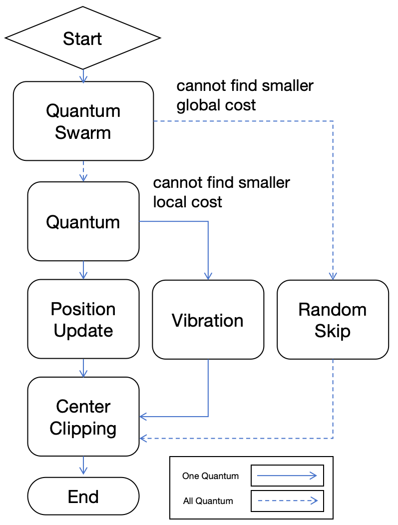
Figure 1: Flowchart of One Iteration in HEO

As Fig.1 shown, in the Halfway Escape Optimization (HEO) algorithm, the swarm is structured as a collection of quantum entities. Each quantum entity iteratively adjusts its position and employs the Center Clipping strategy to satisfy the defined constraints while enhancing the efficiency of the search process. Should the swarm fail to identify a superior global optimum, a random skip is initiated, allowing for a departure from the current trajectory. Concurrently, individual quantum entities engage in a vibration mechanism when local optima are not improved. This action aims to explore beyond the plateaus or local convex hulls, facilitating a more comprehensive exploration of the search space. Details of HEO can be seen in Algorithm 1.

Algorithm 1 Halfway Escape Optimization (HEO)

procedure HEO($k,i_{max},a_{\text{max}},c_{\text{max}},f,p,\text{bound},R$)

     $Q\leftarrow$ list of $k$ quantums with positions,levels and local optimas

     $f_{\text{best}}\leftarrow\min(\{f(q.\text{x})\mid q\in Q\})$, $c_{i}\leftarrow 0$

     $q_{\text{best}}\leftarrow$ quantum in $Q$ with fitness $f_{\text{best}}$

     for $i\leftarrow 1$ to $i_{max}$ do

         for all $q$ in $Q$ do

              update position of $q$

              $f_{q}\leftarrow f(q.\text{x})$

              if $f_{q}<f_{\text{best}}$ then

                  Update $f_{\text{best}},q_{\text{best}}$

                  $c_{i}\leftarrow int(c_{i}/2$)

              else if $f_{q}<f(q.\text{local\_best}.\text{x})$ then

                  Update $q.local\_best$

                  $q.a_{i}\leftarrow int(q.a_{i}/2$)

              else

                  $n\leftarrow N(0,\sigma_{q.x},p)$

                  $q.x$+=$\frac{n}{1+e^{a_{i}}}$

              end if

              center clipping $q.\text{x}$ in $S_{result}$

         end for

         if $q.a_{k}*r_{4}<\frac{a_{max}-1}{2}$ then

              $q.a_{k}$++

         end if

         if $c_{i}>c_{max}$ then

              every quantum $q$ random skip

              $c_{i}\leftarrow 0$

         end if

         $c_{i}$++

     end for

     return $f_{\text{best}}$, $q_{\text{best}}$

end procedure

3.2 Position Update

The mechanism Position Update of HEO, as it is named, is the special way that quantum updates its position for search, which is the fundamentals of all optimization algorithms. Similar to PSO, in HEO, the updates of quantums’ position consider both the local optimum and global optimum. The core concept of the HEO is ”escape”, the quantum in HEO would move towards the opposite direction once the group gets stuck in the local optima, this trait allows HEO to escape from it. First of all, as Fig.2 shows, the HEO is not fully gradient dependent like PSO, HEO only uses fitness or cost for updating the velocity of escape as well as updating the bound of the quantum, which makes HEO find relatively good solutions on the sheer and other narrow landscapes.

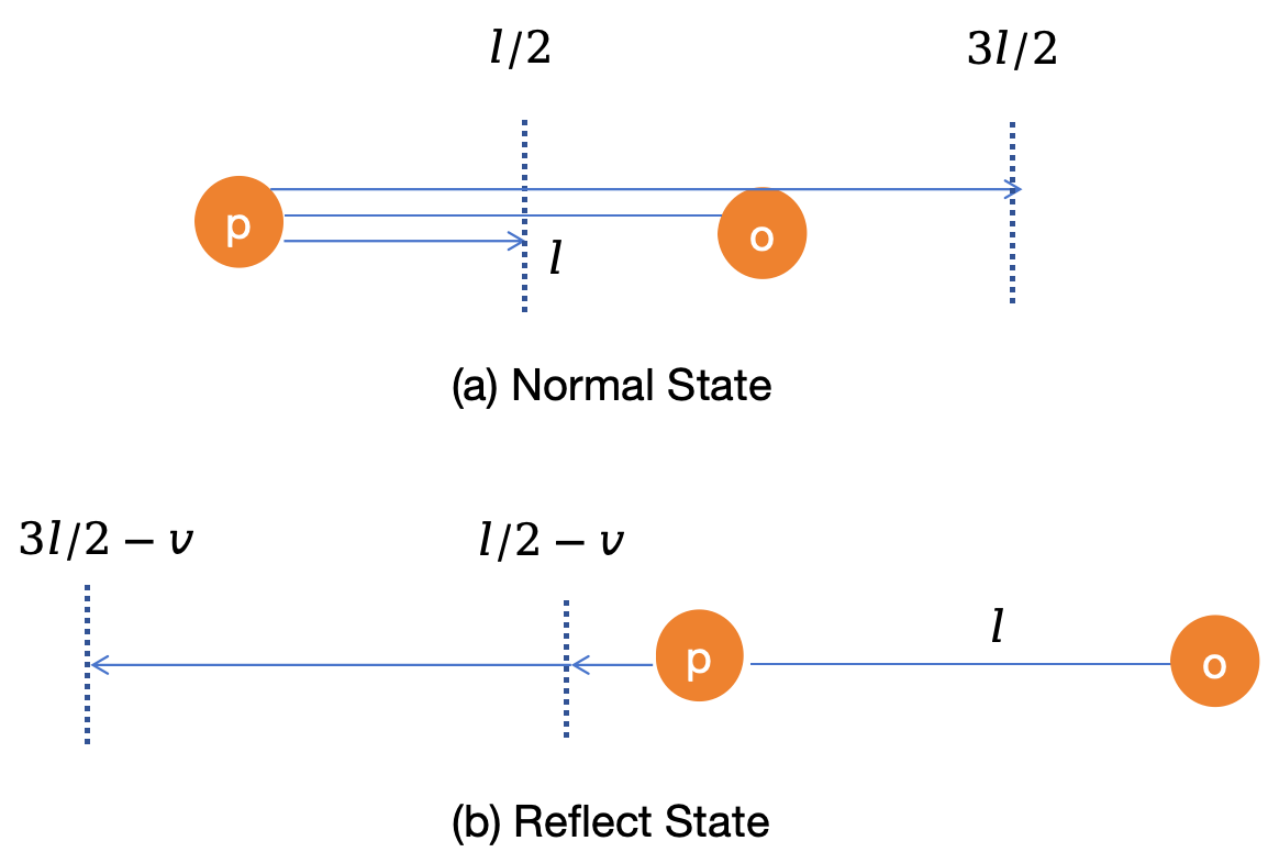
Figure 2: Position Update in HEO

$$x_{i+1}=x_{i}+v_{g}+v_{l},\quad i=1,2,3...N$$ (1)

$$v_{g}=(x_{g}-x_{i}(c_{i}+1)\times r_{1})\times r_{2}\times r_{3}$$ (2)

$$v_{l}=(x_{l}-x_{i}(c_{i}+1)\times r_{1})\times r_{2}(1-r_{3})$$ (3)

In the normal state(a), quantum does not have any velocity. When the escape factor $c_{i}$ is equal to zero the behavior is equivalent to finding the solution surrounding the halfway of optima in equation (1).To be precise, the HEO algorithm would get into reflect state(b) as Fig.2 shows, to find other possible solution spaces. Unlike directly searching randomly, the reflecting state of the HEO’s quantum utilizes the information(which is $c_{i}$ here) from local optima, allowing it to escape from it faster.

$$r_{1}\sim U(1-R,1+R)$$ (4)

$$r_{2}\sim U(0.5,1.5)$$ (5)

$$r_{3}\sim U(0,1)$$ (6)

$$c_{i+1}=\left\{\begin{aligned} 0\quad\quad\quad\quad\quad\quad(\text{when }i=0)\\ c_{i}+1\quad(\text{when }f_{global}>f_{best})\\ c_{i}\mid 2\quad\quad\quad\quad\quad\quad\text{else}\quad\quad\quad\end{aligned}\right.$$ (7)

As for random factors $r_{1}$ and $r_{2}$ shown in equation (4) and equation (5), $r_{1}$ is for controlling the magnitude of an escape step, making HEO escape behaviors more efficient than simple grid search.$r_{2}$ is added to randomize further the process. Both of those two random variables have exception 1 to ensure the feasibility. The random factor $r_{3}$ controls the global weight of this updating process, creating a fan area to search for the solution.

$$\forall A,A=\{s_{1},s_{2}\},T(A)=s^{*},f(s^{*})=f^{*}$$ (8)

$$G_{P}=(S_{P},T),G_{O}=(S_{O},T),G_{H}=(S_{H},T)$$ (9)

$$s_{P}\in S_{P},s_{O}\in S_{O},s_{H}\in S_{O}$$ (10)

Since the HEO originates from PSO, the paper could have a rough insight into its convergence from the aspect of its ancestor. Ignoring the random factors for adding randomness and the escape term contained in the formulas, the HEO has the same way of updating the position as PSO does.

Also, as equation (9) and (10) shown, due to the particles or quantum in the groups, the algebraic structure, being all restricted by the required bound, the group of HEO $G_{H}$, as well as $G_{P}$ in PSO, could both be technically defined as groups with a min function operation $T$ of equation (8). The individual that held local minimum cost is included in the individual’s history, which proves the boundness of it.

Secondly, the individual that has extreme value cost is in the span of the space, ensuring the invertibility of function $T$. Thirdly, as previously motioned, the HEO is the same as PSO without adding an ”escape term” as well as multiplying those factors, making them satisfy the commutative and associative law.

In the case of PSO as well as HEO, the identity element would be the particle or quantum with the lowest cost between two individuals(the local optimum and the current one), while the inverse identity of it would be the current individual, hence the identity as well as the inverse identity exists and unique. In conclusion, the algebraic structures $G_{P}$ and $G_{O}$ are groups.

$$\because O(s_{P})=s_{H}$$ (11)

$$\therefore G_{H}=G_{P}\rtimes G_{O}$$ (12)

Besides, the paper defined an operation or function that could convert element $s_{P}$ to $s_{H}$ in equation (11), and the group $G_{O}$ is a group of different values for scaling in HEO. Additionally, since the individuals are generated randomly, which means there a nearly zero odds for PSO and HEO to have overlap values, make the semi-direct product established [5].

The semidirect product is defined as the multiplication operation of two groups through Cartesian product, where the elements of the two groups are combined in a specific way to form a new group structure[5]. Consequently, the group $G_{H}$ in HEO can be viewed as the outcome of the semi-direct product between $G_{P}$ and the group of the additional term $G_{O}$ in equation (12), the extra term $G_{O}$ is converge due its exception, and the identity $e_{o}$ come from the identities of two groups. As per the definitions, the identity of the group is the local optimum that gets searched and decreases.

The established global convergence of Particle Swarm Optimization (PSO) [3] [19] implies, to a certain extent, the global convergence of HEO with an absence of the escape term ($c_{i}=0$). This conclusion is derived from the fact that the global optimum is achieved through the aggregation of local optima, thus demonstrating a comparable convergence behavior between the two algorithms.

Global convergence in swarm optimization algorithms is the ability of the entire swarm to reach the global optimal solution, as opposed to getting stuck in local optima. This is important because it ensures that the algorithm will find the best possible solution to the problem, which is critical for real-world applications where sub-optimal solutions can lead to subpar performance or failure. In other words, the global convergence of HEO also theoretically proves its effectiveness.

3.3 Vibration

Another behavior of HEO is common in other algorithms including AFSA, when the search is meaningless to making a random step for individual search. Yet those algorithms adopt the strategy, they ignore the influence of size of steps, and those search approaches highly rely on the hyper-parameters tunning. HEO tries to use the standard deviation of positions to judge the magnitude of one random step, creating a relatively stable performance compared to the others, this random search is called Vibration.

$$x_{i+1}=x_{i}+\frac{n}{1+e^{a_{i}}}$$ (13)

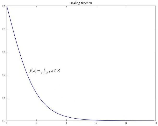
Figure 3: Scaling Function

$$a_{i+1}=\left\{\begin{aligned} a_{i}+1\quad(\text{when }a_{i}*r_{4}<a_{max})\\ a_{i}\mid 2\quad(\text{when }f_{local}<f_{best})\end{aligned}\right.$$ (14)

$$r_{4}\sim U(0,1)$$ (15)

$$n\sim N(0,\sigma_{x_{i}})$$ (16)

Just like the behavior of quantum in physics, with higher energy level $a_{i}$, the quantum would be harder get influenced by others[21], which means smaller oscillations(seen in equation (13) and Fig.3), maintain an extent of diversity in the population. To maintain the convergence of the whole group, the increment of energy level $a_{i}$ only works in a few quantums. Additionally, other scaling approaches to adapting the space of high dimensions with gamma functions are computed much slower than just simply calculating the standard deviation of the position vectors. The reason for using Normal distribution due its universal applicability. According to the central limit theorem, with the increasing of the dimension, the size of the vibration is more approximate to the size of the step in the real situation. Since the HEO does not include periodical functions in this behavior, it cannot defined as oscillations, that’s the reason for its name.

3.4 Center Clipping

Just like quantum entanglement causes quantum attraction, so the distance of quantum escape is finite, the quantum group in HEO would restrict the individuals, ensuring them in a certain area to avoid over-escape by the behavior.

$$S_{result}=S_{bound}\cap S_{group}$$ (17)

$$b_{g}=\|x_{i}-x_{g}\|_{2}\times r_{5}$$ (18)

$$r_{5}\sim U(0,2)$$ (19)

As Fig.4 illustrated, the quantum not only would be restricted by the searching area or constraints $S_{bound}$(the area with (a)) with half of side length $b$, but the group also be restricted by the $S_{group}$. $S_{group}$(the area of (b) in Fig.3)is the search space of the group that HEO allows to search with half of the side length $b_{g}$, the search space in HEO are all in the shape of a square, making it computing faster than calculating sphere. Moreover, as equation (18) shows, this bound of group $S_{group}$ is dependent on the differences between the current quantum’s position and the best one that HEO found. Additionally, this center clipping mechanism uses random factor $r_{5}$, making this bound soft edge and not converge too early and maintain the diversity of the group. The final result of the group gets into the range of $S_{result}$, which is the overlap area of the $S_{group}$ and $S_{bound}$.

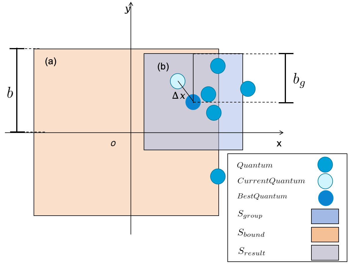
Figure 4: Center Clipping

3.5 Random Skip

The HEO is a swarm algorithm extremely focused on exploration. Except for the vibration behavior that each quantum has, the group itself would be randomly skipped to search the solution with the range of the bound. In equation (19), once the count $c_{i}$ reached $c_{max}$ and then manually defined, the whole group would make this random skip for spanning a totally new space. The reason to use this skipping mechanism is the higher randomness compared to using any periodical function to search in HEO.

$$x_{i}=\frac{x_{i}+\vec{r}}{2}$$ (20)

$$\vec{r}_{j}\in\vec{r}$$ (21)

$$\vec{r}_{j}\sim U(0,b)$$ (22)

As Fig.5 shows, the random skip behavior in HEO allows the entire group of quantum to explore a completely new and random search space, the blue area represents the search space and the orange part is for the constraint. This is achieved by randomly shifting each quantum’s position by a random vector $\vec{r}$ in equation (20). The components of the random vector $\vec{r}_{j}$ are uniformly sampled from the interval $[0,b]$, as shown in equation (22). There are numerous $b$ for $\vec{r}$, hence the shape of the search space also changed with it as in sub-figure(a)(b) does, also the space restricts the constraints as sub-figure(c) is shown. This random skip mechanism enables HEO to explore different regions of the search space and potentially discover new and better solutions.

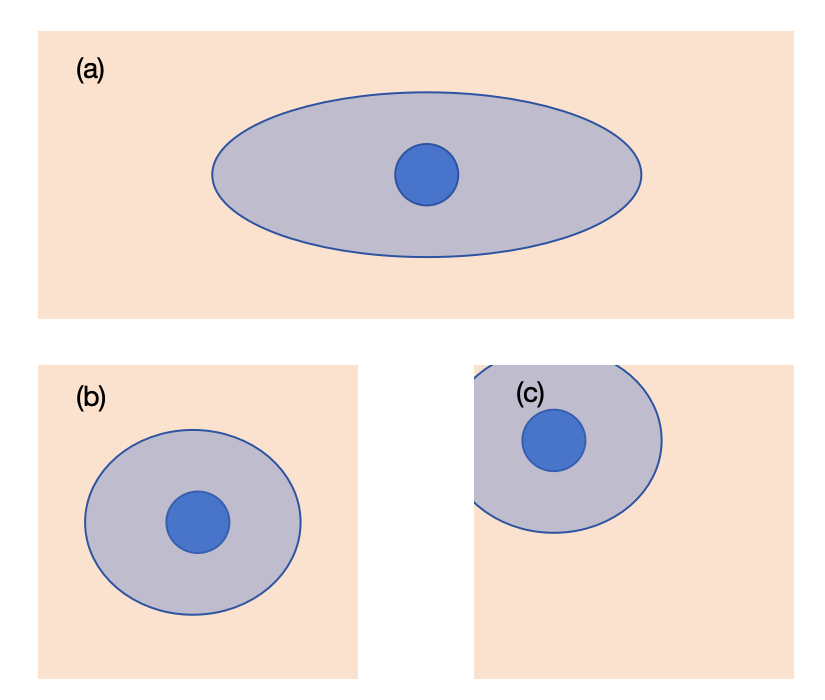
Figure 5: Random Skip

4 Experimental Results

4.1 Experiment Design

The paper selects 14 benchmark functions from famous objective functions that have extensional forms in high dimensions, including 7 unimodal functions in TABLE 1 and 7 multimodal functions in TABLE 2. The experiment would test the performance of classical metaheuristic algorithms including PSO, AFSA, GWO, and GA with the HEO algorithm (check the standard HEO in Algorithm 1) in dimension $p=30$, and searching within 1000 iterations. Each swarm of the testing algorithms have 100 entities, which is common size of the swarm for testing as a rule of thumb. In addition, the experiment is validated 30 times to remove the potential impact caused by randomness.

Name	Function	range	$f_{min}$
Sphere	$F_{1}(x)=\sum_{i=1}^{n}x_{i}^{2}$	[-100,100]	0
Step	$F_{2}(x)=\sum_{i=1}^{n}(x_{i}+0.5)^{2}$	[-100,100]	0
Schwefel 2.21	$F_{3}(x)=\max_{i}|x_{i}|$	[-100,100]	0
Schwefel 2.22	$F_{4}(x)=\sum_{i=1}^{n}|x_{i}|+\prod_{i=1}^{n}|x_{i}|$	[-100,100]	0
Rosenbrock	$F_{5}(x)=\sum_{i=1}^{n-1}\left[(x_{i+1}-x_{i}^{2})^{2}+(x_{i}-1)^{2}\right]$	[-100,100]	0
BentCigar	$F_{6}(x)=x_{1}^{2}+10^{6}\sum_{i=2}^{n}x_{i}^{2}$	[-100,100]	0
Sumsquares2	$F_{7}(x)=\sum_{i=1}^{n}i\cdot x_{i}^{2}$	[-100,100]	0

Table 1: Test Unimodal Functions

Name	Function	range	$f_{min}$
Alpine	$F_{8}(x)=\sum_{i=1}^{n}\left|x_{i}\cdot\sin(x_{i})+0.1x_{i}\right|$	[-100,100]	0
Griewank	$F_{9}(x)=\frac{1}{4000}\sum_{i=1}^{n}x_{i}^{2}-\prod_{i=1}^{n}\cos\left(\frac{x_{i}}{\sqrt{i}}\right)+1$	[-100,100]	0
Rastrigin	$F_{10}(x)=\sum_{i=1}^{n}\left(x_{i}^{2}-10\cos(2\pi x_{i})+10\right)$	[-100,100]	0
Ackley	$F_{11}(x)=20+e-20\exp\left(-0.2\sqrt{\frac{1}{n}\sum_{i=1}^{n}x_{i}^{2}}\right)-\exp\left(\frac{1}{n}\sum_{i=1}^{n}\cos(2\pi x_{i})\right)$	[-100,100]	0
L$\acute{e}$vy	$F_{12}(x)=\sin^{2}(\pi w_{1})+\left(\sum_{i=1}^{n-1}(w_{i}-1)^{2}\left(1+10\sin^{2}(\pi w_{i}+1)\right)\right)+(w_{n}-1)^{2}\left(1+\sin^{2}(2\pi w_{n})\right),w_{i}=1+\frac{x_{i}-1}{4}$	[-100,100]	0
Salomon	$F_{13}(x)=1-\cos(2\pi\sqrt{\sum_{i=1}^{n}x_{i}^{2}})+0.1\sqrt{\sum_{i=1}^{n}x_{i}^{2}}$	[-100,100]	0
Schaffer	$F_{14}(x)=0.5+\frac{1}{D-1}\sum_{i=1}^{D-1}(\sin(\sqrt{x_{i}^{2}+x_{i+1}^{2}})^{2}-0.5)$	[-100,100]	0

Table 2: Test Multimodal Functions

4.2 Trend Analysis

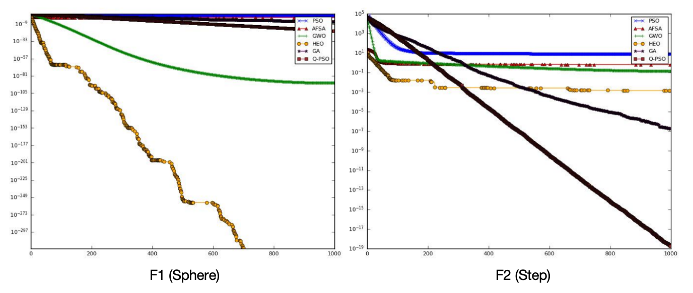
Figure 6: The cost variation in $F_{1}$ and $F_{2}$

In Fig.6, the HEO achieves 0 costs and converges faster than other algorithms in $F_{1}$. The GWO gets the second low-cost. As Table 3 indicates, HEO gets the 0 cost and GWO gets the 1.651e-91 cost, which could also be considered to be almost the global optimum.

The Fig.6 demonstrates the QPSO gets the smallest cost among the others, and the GA and HEO are next in $F_{2}$. As for the convergence, except QPSO, the HEO has get relatively low cost in the beginning to about the 600 iterations. After that, the HEO’s performance is exceeded by the GA. Also, the slope of the GA plot infers the acceptable convergence in further searching, it infers the single constraint conditions might make the HEO hard to converge due to the frequent skip and vibration.

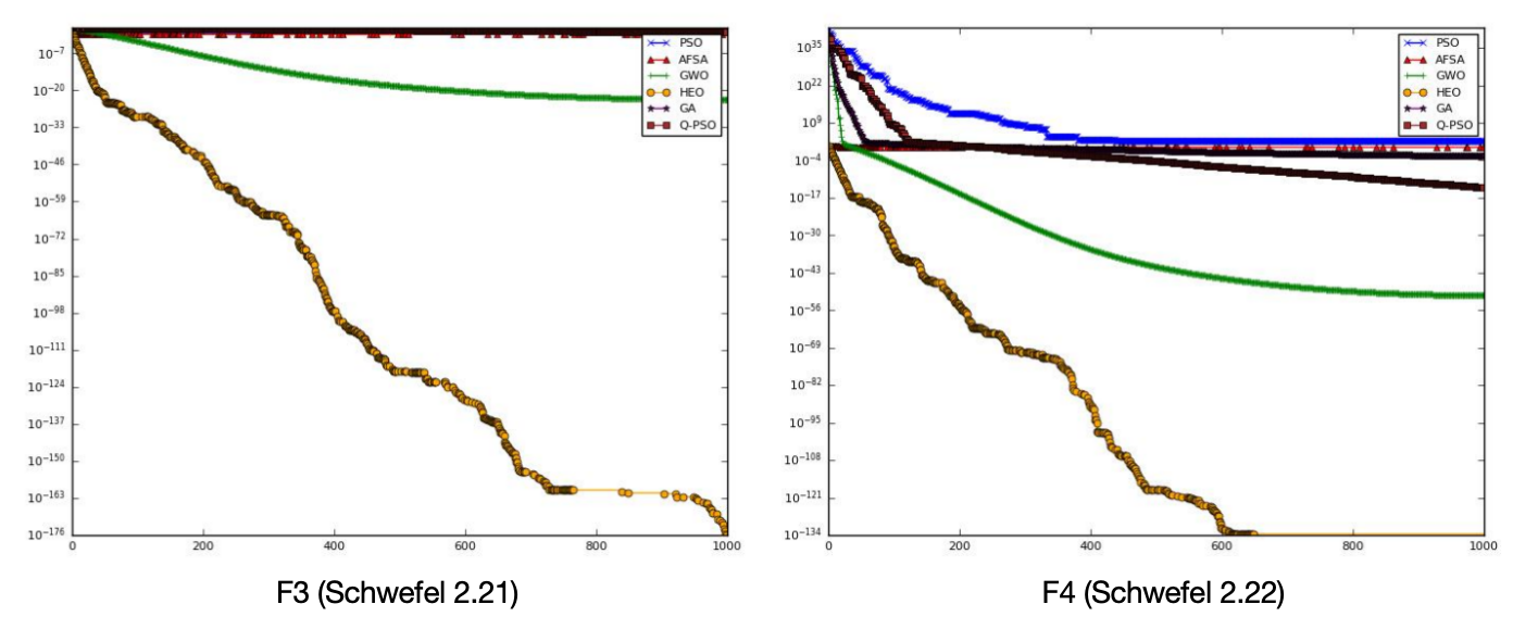
Figure 7: The cost variation in $F_{3}$ and $F_{4}$

For $F_{3}$, the Fig.7 shows the fast convergence of HEO. Other algorithms including GWO seem only to find local optima of the function. Even the cost of GWO is 6.178e-24 (seen in Table 3), which cannot be seen as an ideal situation.

For $F_{4}$, Fig.7 also shows the performances of HEO are much superior to GA, AFSA, and PSO. The HEO only gets around 1e-134 cost, and GWO achieves about 1e-50. The QPSO, AFSA, GWO, and GA express a similar trait on the plot, those algorithms all converge smoothly but stuck in optimums. Adversely, the oscillations of PSO might be brought by the complex landscape of the $F_{4}$ function, and the fluctuations of HEO’s plot might be caused by its unique random mechanism, such as random skip as well as its escape behavior.

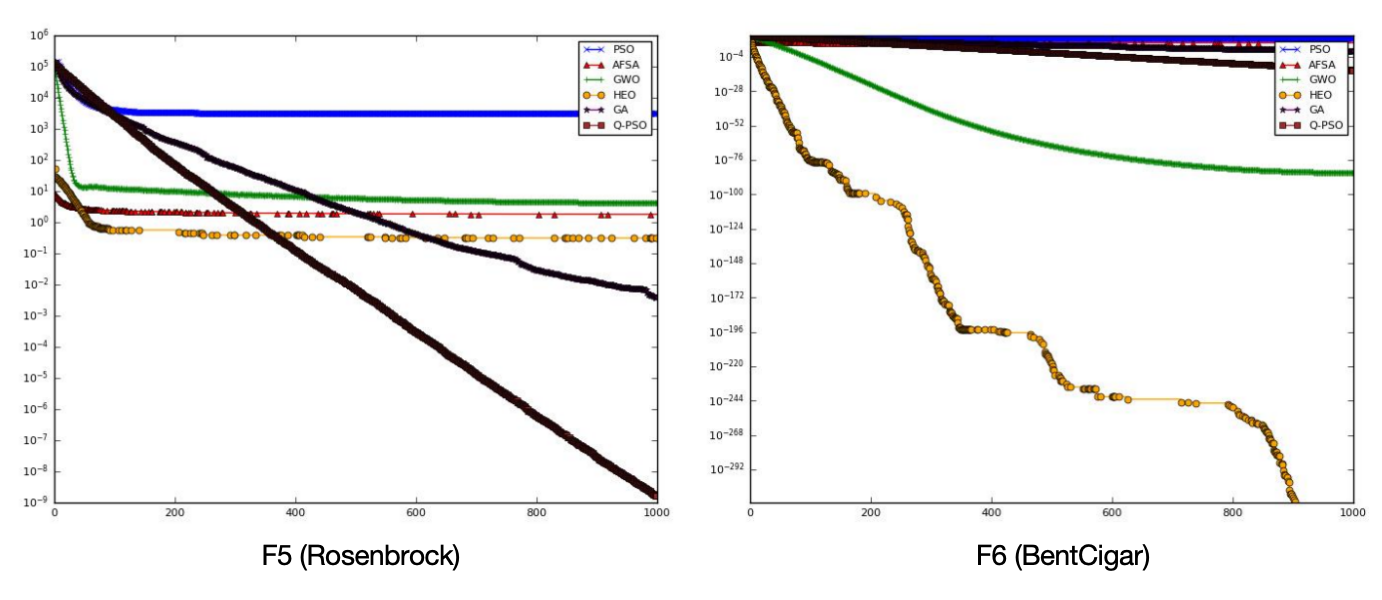
Figure 8: The cost variation in $F_{5}$ and $F_{6}$

For $F_{5}$, Fig.8 shows the majority of algorithms get trapped by the special curve structure, and only GA as well as QPSO gets a good convergence. Besides, the HEO also shows a reasonable cost that is lower than the others.

For $F_{6}$, Fig.8 also shows the HEO finds the global optima, and the GWO algorithm also finds a good solution, as in Table 3, we can observe a cost of 1.893e-85 cost. Other algorithms except GA do not have apparent tendency and they all converge too early as the plot shows.

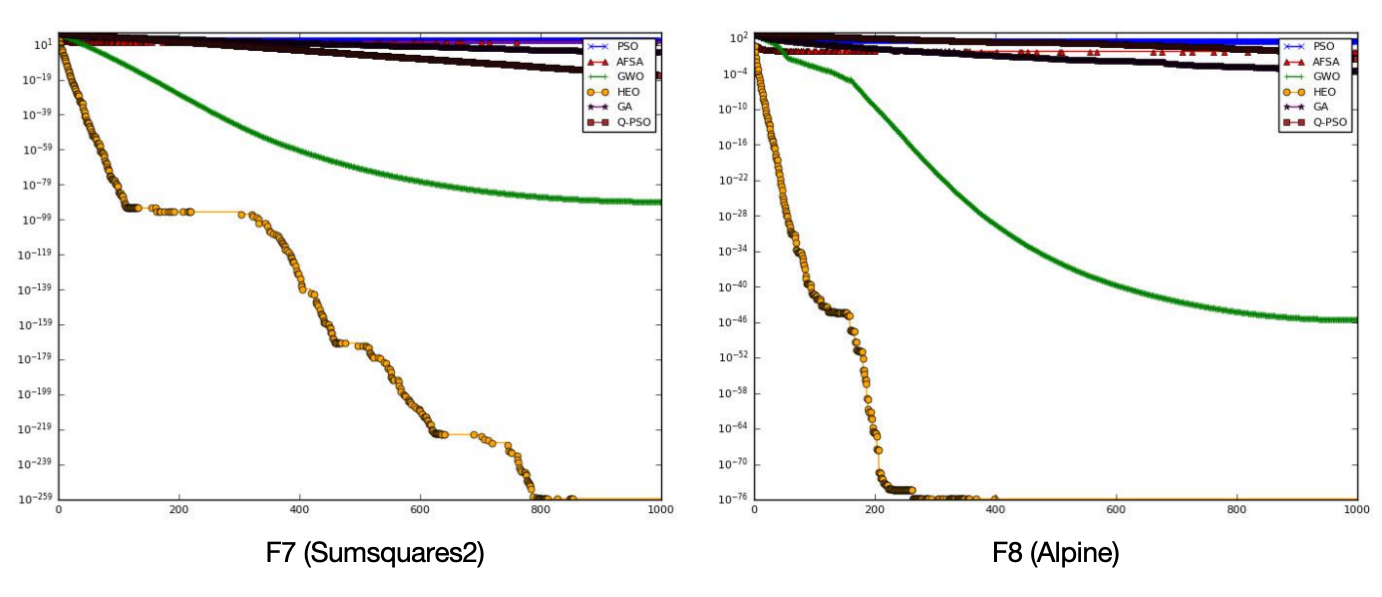
Figure 9: The cost variation in $F_{7}$ and $F_{8}$

For $F_{7}$, the Fig.9 shows the HEO gets a good solution, and GWO follows after it. As for the convergence, HEO converges with the fastest rate, and GWO gets the second fastest rate, notwithstanding the AFSA getting the smallest cost in the first few iterations.

For $F_{8}$, Fig.9 also shows the HEO gets the best performance compared to other algorithms, and GWO gets the second-best performance at around 1e-45 cost. Unlike HEO performs in other functions, the HEO gets a gentle plot shape, which might caused by the smooth landscape of the $F_{8}$.

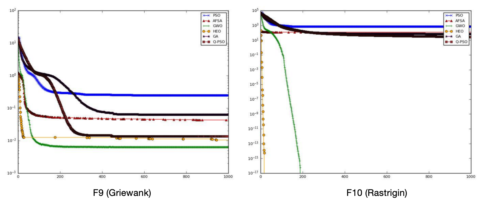
Figure 10: The cost variation in $F_{9}$ and $F_{10}$

For $F_{9}$, Fig.10 illustrates all algorithms that encounter the difficulty of finding The global optima. The $F_{9}$, Griewank, is a complex function. With p=30, the algorithms are easy to trap in a single convex hull that does not contain the best solution. The HEO and GWO get approximate costs, but HEO converge faster and get slightly lower costs.

For $F_{10}$, Fig.10 also shows that GWO as well as HEO both find the global optimum. For analyzing the convergence, the HEO finds the solution faster than the GWO.

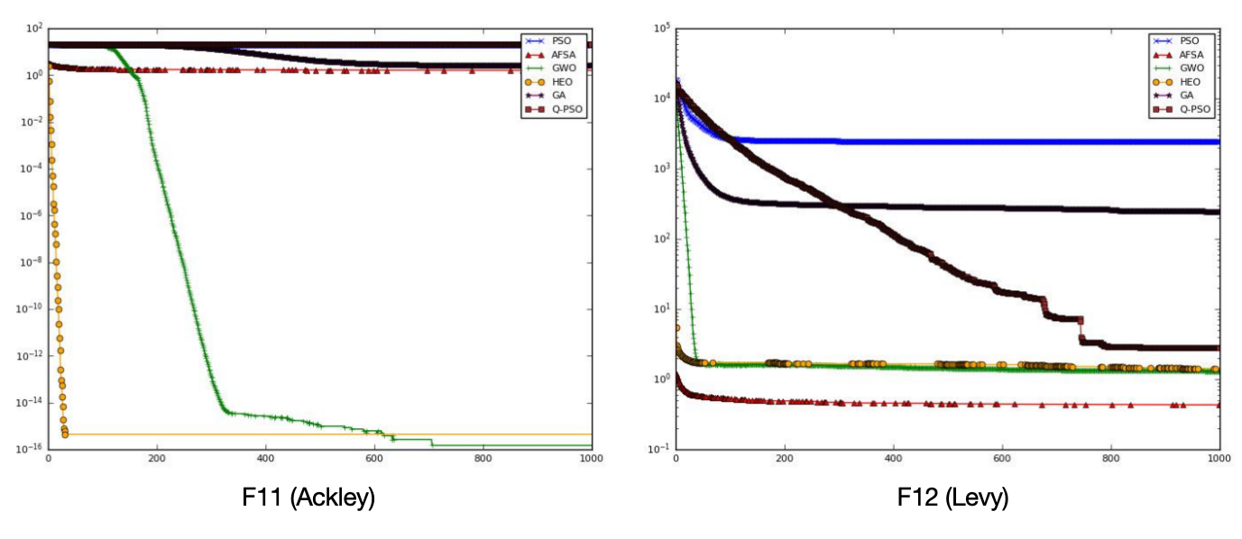
Figure 11: The cost variation in $F_{11}$ and $F_{12}$

For $F_{11}$, Fig.11 shows HEO and GWO both get a reasonable cost around 1e-16, but do not get full convergence. The possible reason for explaining this result could be the hollows of the Ackley function $F_{11}$ in high dimension[2]. Those hollow landscapes with the same cost might be the issue that prevents further convergence of algorithms.

For $F_{12}$, Fig.11 also shows that the AFSA gets the lowest cost and then follows with GWO and HEO. All of the testing algorithms including AFSA do not perform well. The L$\acute{e}$vy functions is a folding bent shape function with some sheer landscapes, which might indicate a drawback for HEO.

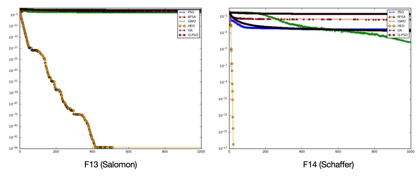
Figure 12: The cost variation in $F_{13}$ and $F_{14}$

For $F_{13}$, Fig.12 shows the HEO gets the best result, which is near the global optimum. Salomon function $F_{13}$ is another sheer function but with an extent of convexity, making HEO able to find the solution.

For $F_{14}$, Fig.12 also shows the HEO found the best solution in the first few iterations. Besides, the GWO has a small inclination to converge further and possibly to find the global optima.

$$\lim_{i\to\infty}x_{i+1}-x_{i}=0$$ (23)

$$\lim_{i\to\infty}E(v_{g})=\frac{(x_{g}-x_{i})}{2}=0\quad(c_{i}=0)$$ (24)

$$\lim_{i\to\infty}E(v_{l})=\frac{(x_{l}-x_{i})}{2}=0\quad(c_{i}=0)$$ (25)

From analysis of 14 benchmark functions, illustrates Halfway Escape Optimization (HEO) gets successful convergences on each case, which validates with the assumption in equation (23). For an ideal situation, the paper could further validate this result by conducting from the equations (1) (2) and (3). When the escape value $c_{i}=0$, and $i$ approximate the infinity, which means the global optimum $x_{g}$ as well as $x_{l}$ should be equal to $x_{i}$, since $x_{i+1}=x_{i}$ shown in equation (23). Besides, the exception value of the random factor is all one except the factor $r_{3}$, which brings a 1/2 scaling.

$$\lim_{i\to\infty}x_{i+1}-x_{i}=E(v_{l})+E(v_{h})=\frac{(x_{l}-x_{i})+(x_{g}-x_{i})}{2}=0$$ (26)

In summary, as the (26) shows, the paper could summarize the ideal situation of the HEO’s exception value as equations (24) (25). By substituting these two terms back into equation (1), the paper can demonstrate the validity of this equation (23). In other words, the HEO could converge once it finds a better optimum,which proves its convergence in another aspect.

4.3 Experimental Comparison

	PSO	AFSA	GWO	HEO	GA	QPSO
$F_{1}$	3.545e+02	7.847e-01	1.651e-91	0.000e+00	8.814e-07	1.465e-19
$F_{2}$	7.943e+00	7.992e-01	1.416e-01	1.344e-03	1.742e-07	1.880e-19
$F_{3}$	1.420e+01	4.495e-01	6.178e-24	1.302e-176	5.579e+00	2.303e+00
$F_{4}$	8.246e+02	3.912e+00	1.622e-51	2.498e-134	4.592e-03	3.713e-14
$F_{5}$	3.168e+03	2.235e+00	4.271e+00	3.112e-01	3.817e-03	1.603e-09
$F_{6}$	1.022e+09	8.106e+05	1.893e-85	0.000e+00	1.077e+00	6.314e-14
$F_{7}$	2.470e+03	3.790e+02	2.168e-89	3.531e-259	4.843e-04	4.084e-17
$F_{8}$	3.381e+01	7.514e-01	2.441e-46	1.299e-76	3.697e-04	4.062e-02
$F_{9}$	0.247727	0.053917	0.006319	0.010466	0.064001	0.013684
$F_{10}$	715.590208	137.192018	0.000000	0.000000	67.088411	27.315077
$F_{11}$	2.000e+01	1.811e+00	1.480e-16	4.440e-16	2.665e+00	2.088e+01
$F_{12}$	2439.240184	0.544817	1.314077	1.421046	245.547882	2.834483
$F_{13}$	4.046e+00	2.954e-01	5.659e-02	9.341e-99	3.357e+00	3.932e-01
$F_{14}$	0.002472	0.050465	0.000076	0.000000	0.001709	0.186564

Table 3: Mean Costs of the Algorithms

The bold text in Table 3 is the smallest cost for one objective function. As the overall result that Table 3 shows, the HEO gets a better comprehensive performance than PSO, AFSA, GWO, GA, and QPSO in major benchmark functions $F_{1}$ to $F_{14}$, and get the minimum costs over 9 functions. On another side, HEO gets a relatively bigger cost in $F_{2}$, $F_{5}$, and $F_{12}$, which might infer the disadvantages of using escape and skip mechanisms in HEO.

	PSO	AFSA	GWO	HEO	GA	QPSO
Unimodal Functions	5.7142	4.5714	2.7142	1.5714	3.7142	2.7142
Multimodal Functions	5.4285	3.5714	1.5714	1.5714	4.0000	4.1428
Total Rank$(F_{1}-F_{14})$	5.5714	4.0714	2.1428	1.5714	3.8571	3.4285

Table 4: The Average Ranks of the Costs

For a more precise analysis, the paper conducts a straightforward rank aggregation procedure on the data presented in Table 3. Algorithms with lower associated costs are accorded higher ranks within this aggregation. The resulting aggregated rank data is displayed in Table 4. In Table 4, the Halfway Escape Optimization (HEO) achieves the highest rank across both unimodal functions (encompassing $F_{1}-F_{7}$) and multimodal functions (encompassing $F_{8}-F_{14}$). This suggests that HEO exhibits similar performance compared to the Grey Wolf Optimizer (GWO) specifically in handling multimodal Functions, it also demonstrates competitive performance relative to the other six algorithms tested in unimodal functions, even in scenarios involving relatively complex functions.

	PSO	AFSA	GWO	HEO	GA	QPSO
$F_{1}$	2.732496	136.057096	74.678300	18.509185	9.189708	25.709296
$F_{2}$	3.307250	150.451374	76.191960	20.107816	10.300027	26.042222
$F_{3}$	0.522904	36.712690	34.066304	8.800284	4.023997	10.214057
$F_{4}$	1.587224	86.004913	72.936023	15.730473	8.095256	24.084705
$F_{5}$	6.240265	237.248756	79.063583	25.920876	13.020591	29.193232
$F_{6}$	2.916587	139.673755	75.215040	18.904487	9.627195	25.440708
$F_{7}$	15.078621	509.393016	87.199845	43.967146	21.811757	37.721174
$F_{8}$	1.059602	63.582046	43.069062	12.031251	6.521126	13.315242
$F_{9}$	10.000640	315.942743	53.234886	31.335585	15.717625	22.645855
$F_{10}$	10.626591	309.697071	83.785108	35.644457	17.775824	33.821670
$F_{11}$	12.349613	381.549480	85.610975	38.228737	19.336686	34.786341
$F_{12}$	7.995789	266.661428	50.095542	27.491028	14.171460	20.122009
$F_{13}$	3.320846	45.687899	77.897484	19.997064	10.503721	26.490371
$F_{14}$	7.923606	273.046009	51.550709	26.627504	14.288681	20.465703

Table 5: Search Time(s/1000 iters) of the Algorithms

As for consider about the efficiency, based on the data from Table 5, the search time of five algorithms in those functions always shows a relationship that: $T_{PSO}<T_{GA}<T_{HEO}\approx T_{QPSO}<T_{GWO}\approx T_{AFSA}$. In conclusion, the HEO demonstrates an acceptable search time as well as a good performance among test functions except for $F_{12}$, but further validation of its effectiveness is still needed. For example, for have a more comprehensive of view, further tests could focus on testing HEO in other objective functions and various dimensions instead of just 30. This broadened experiment could give a more precise evaluation of the HEO.

5 Simple Test in Traveling Salesman Problem (TSP)

The Traveling Salesman Problem (TSP) is a well-known optimization problem in computer science and operations research. It involves finding the shortest route for a salesman to visit a set of cities exactly once. TSP is an NP-hard problem, which means that as the problem size increases, the time complexity of solving it will significantly increase, making it a well case for testing HEO.

This study aims to evaluate the effectiveness of the HEO algorithm in solving general Path Planning Problems. To do so, the algorithm is compared against Tabu Search and Random Search, using randomly generated datasets with 25, 50, and 100 cities with 2-dimensional position ranges within [-10,10]. The performance of these algorithms is assessed based on 100 iterations of searching and starts with the first city.

Tabu Search is a popular heuristic algorithm widely used in combinatorial optimization problems[9]. It systematically explores the search space while avoiding local optima through the utilization of a ”tabu list” that prevents revisiting recently examined solutions. This mechanism allows for the exploration of new regions and the discovery of improved solutions. Tabu Search has gained prominence due to its efficacy in solving intricate optimization problems, making it a well-tested algorithm for comparison. Random Search is another usually used baseline for evaluation in TSP, which was first used as a benchmark in 1986 [10].

In Fig.13, the path taken by the algorithms with 25 cities is depicted for a clear overview. Additionally, Table 6 demonstrates that the HEO algorithm consistently outperforms Random Search in terms of achieving shorter distances across all test cases. As the number of cities increases, Tabu Search experiences a significant increase in execution time. For instance, when there are 25 cities, the Tabu Search only costs 1.334546 seconds for 100 iterations, which is a shorter time compared to HEO. But when the number of cities is larger than 25, the HEO shows a relatively shorter time for searches. This highlights the potential of HEO as an alternative for more complex scenarios.

Overall, this research highlights the effectiveness of the HEO algorithm in general Path Planning Problems, as verified through the comparison with Tabu Search and Random Search methodologies. The findings indicate that HEO offers acceptable performance and potential. Also, compared to specialized algorithms that specifically focus on local search, such as Simulated Annealing (SA) [14], HEO performs worse than Tabu Search. The Halfway Escape Optimization (HEO) has a relatively weaker capability for local search. However, the complexity of this test is relatively simple compared to the real-time applications.

Further validations of the HEO algorithm’s effectiveness in TSP can be conducted through more complex scenarios. For example, real-world problems, such as route planning for drone delivery, can be used to verify the algorithm’s capabilities [1]. Additionally, comparing HEO to other swarm optimization algorithms in form of TSP, can provide insights into the algorithm’s strengths and weaknesses in different contexts. Future research can also investigate the impact of different parameters, such as the scaling radius $R$ in (4), on the algorithm’s performance. Nonetheless, the results presented in this study demonstrate the potential of HEO as a promising algorithm for solving TSP and other path planning problems.

Methods	Cities	Distance	Search Time(s/100 iters)
Tabu	25	100.626530	1.334546
HEO	25	133.276518	3.973852
Random	25	198.440632	0.013264
Tabu	50	172.474598	6.105021
HEO	50	300.411801	3.707406
Random	50	447.679963	0.022514
Tabu	100	301.104570	88.637227
HEO	100	674.661410	10.675231
Random	100	923.988814	0.079656

Table 6: The TSP performance

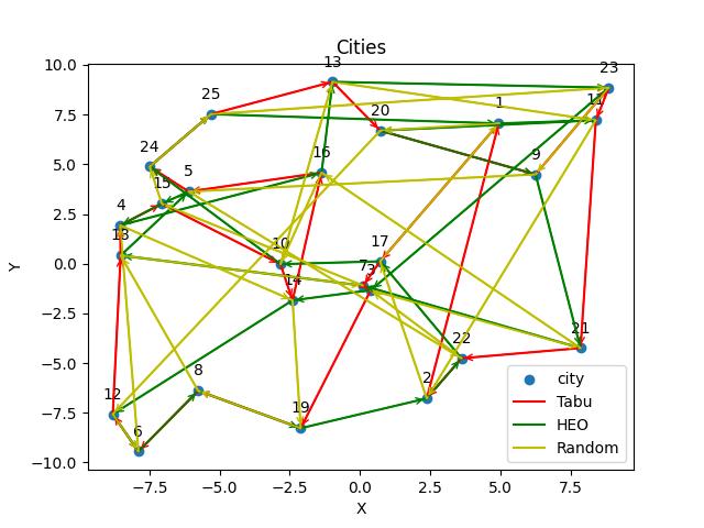
Figure 13: The Paths of the Methods in TSP

6 Discussion

The experimental results indicate that HEO outperforms other algorithms in terms of convergence speed and solution quality across a range of benchmark functions. The algorithm’s ability to balance exploration and exploitation, coupled with its adaptive strategies, has resulted in competitive performance in challenging optimization landscapes. The TSP test also validates its availability in path-planning applications.

The discussion of TSP highlights the effectiveness of the HEO algorithm in general Path Planning Problems, as verified through the comparison with Tabu Search and Random Search methodologies. When dealing with a relatively complex situation, the findings indicate that HEO offers acceptable performance and potential, particularly in terms of searching speed.

However, whether the performance of the HEO is enough to deal with real-time TSPs still questionable, the applications of HEO may have to be more focused on realms like industrial parts manufacturing instead of a more dynamic environment. Besides, some special functions like L$\acute{e}$vy would still be an issue for HEO to explore the solutions.

7 Conclusion

Through its quantum-inspired metaheuristic, Halfway Escape Optimization (HEO) demonstrates adaptability, efficiency, and effectiveness in navigating rugged landscapes, high-dimensional search spaces, and multimodal problems. The algorithm’s unique energy-driven behavior, vibration strategies, and exploratory mechanisms contribute to its ability to balance exploration and exploitation, leading to fast convergence rates and high-quality solutions.

Moreover, the adaptability of the HEO algorithm allows it to be applied to dynamic environments where the objective functions or constraints may change over time. By continuously adapting its search strategy and updating the particle positions, HEO can effectively track and respond to changing optimization landscapes, ensuring that high-quality solutions are maintained even in dynamic scenarios, including TSP applications.

Overall, the Halfway Escape Optimization algorithm has demonstrated its effectiveness and adaptability in addressing complex optimization challenges. Future work could focus on further refining the algorithm’s parameters and exploring its application in practical optimization problems. Additionally, the algorithm could be extended to address multi-objective optimization problems and dynamic environments or change the strategy of escape and skip, further enhancing its versatility and applicability.

Declaration of competing interest

The authors declare that they have no known competing financial interests or personal relationships that could have appeared to influence the work reported in this paper.

CRediT authorship contribution statement

Jiawen Li: Conceptualization, Methodology, Writing-Original Draft, Writing-Editing. Anwar PP Abdul Majeed: Supervision, Writing-Review, Validation Pascal Lefevre: Supervision, Writing-Review, Validation

Data availability

The experiment is data-available for replications after the relevant paper get published, provide the source code of HEO in: https://github.com/Spike8086/HEO.git, provide data of result and the notebook of experiment in: https://www.kaggle.com/code/spike8086/heo-formal-ver, and give the code for TSP test:https://www.kaggle.com/code/spike8086/heo-for-tsp

Symbols

Symbol	Definition
$i$	The Current Number of Iteration
$N$	The Total Number of Iteration/Normal Distribution
$x_{i}$	The Position of The $i_{th}$ Quantum
$v_{l}$	The Global Velocity of The Quantum
$v_{g}$	The Local Velocity of The Quantum
$c_{i}$	The Escape Factor
$r_{1}$	The Random Factor for Escape Term
$r_{2}$	The Random Factor for The Whole Position Update
$r_{3}$	The Random Global Weight
$R$	The Radius for Scaling the Range of $r_{1}$
$f_{global}$	The Global Optimum of the Swarm
$f_{local}$	The Local Optimum of the Quantum
$A$	A Set Composed of the Positions of Two Quantum
$s$	The Position of Any Single Sample(Quantum/Particle)
$T$	Customized Function That Return the Optimum
$G$	Any Group
$S$	Any Set of Samples
$O$	Scaling Operation in HEO
$a_{i}$	Energy Level of Quantum
$r_{4}$	The Random Factor for Increment of Energy Level
$\sigma_{x_{i}}$	The Standard Deviation of Vector $x_{i}$
$b_{g}$	The Side Length/Radius of the Extra Constraint Area
$r_{5}$	The Random Factor for the Soft Edge
$b$	The Side Length/Radius of the Required Constraint Area
$\vec{r}$	The Random Factors for Random Skipping
$f^{*}$	The Function Value of the Optimum
$s^{*}$	The Solution of the Optimum

Abbreviation

Abbreviation	Description
HEO	Halfway Escape Optimization
TSP	Traveling Salesman Problem
GA	Genetic Algorithm
PSO	Particle Swarm Optimization
ACO	Ant Colony Optimization
VRP	Vehicle Routing Problem
DE	Differential Evolution
AFSA	Artificial Fish Swarm Algorithm
FA	Firefly Algorithm
QPSO/Q-PSO	Quantum behaved Particle Swarm Optimization
GWO	Grey Wolf Optimizer
SSA	Salp Swarm Algorithm
SA	Simulated Annealing

References

- Dro [2022] (2022). Solving the vehicle routing problem with drone for delivery services using an ant colony optimization algorithm. Advanced Engineering Informatics, 51, 101536. doi:https://doi.org/10.1016/j.aei.2022.101536.
- Cai et al. [2020] Cai, W., Yang, L., & Yu, Y. (2020). Solution of ackley function based on particle swarm optimization algorithm, . URL: https://ieeexplore.ieee.org/document/9213634.
- Clerc & Kennedy [2002] Clerc, M., & Kennedy, J. (2002). The particle swarm - explosion, stability, and convergence in a multidimensional complex space. IEEE Transactions on Evolutionary Computation, 6, 58–73. doi:10.1109/4235.985692.
- Dorigo et al. [1996] Dorigo, M., Maniezzo, V., & Colorni, A. (1996). Ant system: optimization by a colony of cooperating agents. IEEE Transactions on Systems, Man and Cybernetics, Part B (Cybernetics), 26, 29–41. doi:10.1109/3477.484436.
- Dummit & Foote [1991] Dummit, D. S., & Foote, R. M. (1991). Abstract Algebra. Englewood Cliffs, NJ: Prentice Hall.
- Eberhart & Kennedy [1995] Eberhart, R., & Kennedy, J. (1995). A new optimizer using particle swarm theory, . doi:10.1109/mhs.1995.494215.
- Elegbede [2005] Elegbede, C. (2005). Structural reliability assessment based on particles swarm optimization. Structural Safety, 27, 171–186. URL: https://www.sciencedirect.com/science/article/pii/S0167473004000499. doi:https://doi.org/10.1016/j.strusafe.2004.10.003.
- ELGebaly [2019] ELGebaly, A. E. (2019). Optimized design of single tum transformer of distributed static series compensators using fem based on ga. In 2019 21st International Middle East Power Systems Conference (MEPCON) (pp. 1133–1138). doi:10.1109/MEPCON47431.2019.9008227.
- Glover [1986] Glover, F. (1986). Future paths for integer programming and links to artificial intelligence. Computers & Operations Research, 13, 533–549. doi:10.1016/0305-0548(86)90048-1.
- Grefenstette [1986] Grefenstette, J. J. (1986). Optimization of control parameters for genetic algorithms. IEEE Transactions on Systems, Man, and Cybernetics, 16, 122–128. doi:10.1109/TSMC.1986.289288.
- Han et al. [2018] Han, H., Lu, W., Zhang, L., & Qiao, J. (2018). Adaptive gradient multiobjective particle swarm optimization. IEEE Transactions on Cybernetics, 48, 3067–3079. doi:10.1109/TCYB.2017.2756874.
- Holland [1975] Holland, J. H. (1975). Adaptation in Natural and Artificial Systems: An Introductory Analysis with Applications to Biology, Control, and Artificial Intelligence. Complex Adaptive Systems.
- Karp [2010] Karp, R. M. (2010). Reducibility among combinatorial problems. In M. Jünger, T. M. Liebling, D. Naddef, G. L. Nemhauser, W. R. Pulleyblank, G. Reinelt, G. Rinaldi, & L. A. Wolsey (Eds.), 50 Years of Integer Programming 1958-2008: From the Early Years to the State-of-the-Art (pp. 219–241). Berlin, Heidelberg: Springer Berlin Heidelberg. URL: https://doi.org/10.1007/978-3-540-68279-0_8. doi:10.1007/978-3-540-68279-0_8.
- Kirkpatrick et al. [1983] Kirkpatrick, S., Gelatt, C. D., & Vecchi, M. P. (1983). Optimization by simulated annealing. Science, 220, 671–680. URL: https://www.science.org/doi/abs/10.1126/science.220.4598.671. doi:10.1126/science.220.4598.671. arXiv:https://www.science.org/doi/pdf/10.1126/science.220.4598.671.
- Li et al. [2002] Li, X. L., Shao, Z. J., & Qian, J. X. (2002). An optimizing method based on autonomous animats: Fish-swarm algorithm. Systems Engineering - Theory and Practice, 22, 32--38. doi:10.12011/1000-6788(2002)11-32.
- Mirjalili et al. [2017] Mirjalili, S., Gandomi, A. H., Mirjalili, S. Z., Saremi, S., Faris, H., & Mirjalili, S. M. (2017). Salp swarm algorithm: A bio-inspired optimizer for engineering design problems. Advances in Engineering Software, 114, 163–191. doi:10.1016/j.advengsoft.2017.07.002.
- Mirjalili et al. [2014] Mirjalili, S., Mirjalili, S. M., & Lewis, A. (2014). Grey wolf optimizer. Advances in Engineering Software, 69, 46–61. doi:10.1016/j.advengsoft.2013.12.007.
- Omkar et al. [2009] Omkar, S., Khandelwal, R., Ananth, T., Narayana Naik, G., & Gopalakrishnan, S. (2009). Quantum behaved particle swarm optimization (qpso) for multi-objective design optimization of composite structures. Expert Systems with Applications, 36, 11312--11322. URL: https://www.sciencedirect.com/science/article/pii/S0957417409002978. doi:https://doi.org/10.1016/j.eswa.2009.03.006.
- Rapaić & Željko Kanović [2009] Rapaić, M. R., & Željko Kanović (2009). Time-varying pso – convergence analysis, convergence-related parameterization and new parameter adjustment schemes. Information Processing Letters, 109, 548--552. URL: https://www.sciencedirect.com/science/article/pii/S0020019009000350. doi:https://doi.org/10.1016/j.ipl.2009.01.021.
- Saw et al. [2023] Saw, B. K., Bohre, A. K., Jobanputra, J. H., & Kolhe, M. L. (2023). Solar-dg and dstatcom concurrent planning in reconfigured distribution system using apso and gwo-pso based on novel objective function. Energies, 16. URL: https://www.mdpi.com/1996-1073/16/1/263. doi:10.3390/en16010263.
- Sommerfeld [1916] Sommerfeld, A. (1916). Zur quantentheorie der spektrallinien. Annalen der Physik, 356, 1–94. doi:10.1002/andp.19163561702.
- Storn & Price [1997] Storn, R., & Price, K. (1997). Differential evolution – a simple and efficient heuristic for global optimization over continuous spaces. Journal of Global Optimization, 11, 341–359. doi:10.1023/a:1008202821328.
- Tanakitkorn et al. [2014] Tanakitkorn, K., Wilson, P. A., Turnock, S. R., & Phillips, A. B. (2014). Grid-based ga path planning with improved cost function for an over-actuated hover-capable auv. In 2014 IEEE/OES Autonomous Underwater Vehicles (AUV) (pp. 1--8). doi:10.1109/AUV.2014.7054426.
- Vázquez et al. [2013] Vázquez, J. C., Valdez, F., & Melín, P. (2013). Comparative study of particle swarm optimization variants in complex mathematics functions. Studies in computational intelligence, (p. 223–235). doi:10.1007/978-3-642-33021-6_18.
- Wang et al. [2019] Wang, Y., Zhang, H., & Zhang, G. (2019). cpso-cnn: An efficient pso-based algorithm for fine-tuning hyper-parameters of convolutional neural networks. Swarm and Evolutionary Computation, 49, 114--123. URL: https://www.sciencedirect.com/science/article/pii/S2210650218310083. doi:https://doi.org/10.1016/j.swevo.2019.06.002.
- Yang [2009] Yang, X.-S. (2009). Firefly algorithms for multimodal optimization, . (p. 169–178). doi:10.1007/978-3-642-04944-6_14.